Idiosyncratic Risk, Government Debt and Inflation

Abstract

How does public debt matter for price stability? If it is useful for the private sector to insure idiosyncratic risk, government debt expansions can increase the natural rate of interest and create inflation. As I demonstrate using a tractable model, this holds in the presence of an active Taylor rule and does not require the absence of future fiscal consolidation. Further analysis using a full-blown 2-asset HANK model reveals the quantitative magnitude of the mechanism to crucially depend on the structure of the asset market: under standard assumptions, the effect of public debt on the natural rate is either overly strong or overly weak. Employing a parsimonious way to overcome this issue, my framework suggests relevant effects of public debt on inflation under active monetary policy: In particular, persistently elevated public debt may make it harder to go the “last mile of disinflation” unless central banks explicitly take its effect on the neutral rate into account.

Keywords: Monetary policy, Fiscal Policy, Inflation, HANK
JEL Classification: E31, E52, E63

1 Introduction

In the aftermath of the Covid-19 pandemic as well as the economic fallout following Russia’s invasion of Ukraine, public debt levels have risen to historic highs in many advanced countries. Should central banks be concerned about this? In standard macroeconomic models, Ricardian Equivalence suggest that they should only if said debt is “unfunded”, i.e. not backed by future government revenue. In the words of ECB board member Schnabel (2022), “if governments do not credibly signal their commitment to responsible fiscal policies, the private sector may eventually expect that higher inflation is needed to ensure the sustainability of public debt”. But if the debt is expected to be eventually paid back by budget surpluses at some point in the future, it doesn’t need to affect the conduct of their policies. Arguably, potential support for this notion may be lent by the observation that conventional monetary policy appears to have been broadly successful in reigning in the recently high inflation, although concerns remain that “the disinflation process during the last mile will be more uncertain, slower and bumpier” (Schnabel, 2023).
However, things get more complex if government bonds have additional value for the private sector, e.g. as a means of insurance against idiosyncratic risk. In that case, the amount of public debt will generally affect the inflation-neutral interest rate, as it imperfectly crowds out private demand and induces households to require a higher real return if they are to hold more government debt. Thus, if a central bank pursues an interest rate rule satisfying the Taylor principle, this can create inflation even if a country’s fiscal authority is committed to raise enough surpluses to eventually pay back the debt (i.e. it is “funded”). All that is needed for this is the monetary authority not (or imperfectly) adjusting its reaction function in response to the government debt expansion.
I first establish these results using a tractable New Keynesian model enriched with idiosyncratic income risk. As obtaining analytical results for such models is notoriously difficult in the presence of a positive net supply of assets, this framework naturally relies on many simplistic assumptions, such as households being ex-ante identical and subject to income risk only in a single period. However, this simplicity also has the virtue of clarifying that the mechanism does not rely on fiscal policy inducing any ex-ante redistribution towards constrained households, a channel that received substantial attention by the recent literature on Heterogeneous Agents New Keynesian (HANK) models. Additional assumptions elucidate that it does neither require the government to consume the resources it acquires through issuing debt nor is it relying on distortionary taxation to consolidate its finances, both of which could also affect inflation in Ricardian models. Furthermore, it is consistent with the fiscal authority being committed to raise any amount of surplus necessary to pay back its debt.
Naturally, the analytical insights beget the question to what extent they may be quantitatively relevant. As their general equilibrium nature precludes empirical identification, I approach this issue by relying on a calibrated 2-asset HANK model, in which households require liquid assets to insure themselves against skill-, unemployment- as well as business risk but also have access to illiquid capital assets yielding higher returns.
The calibrated framework matches well various micro-data moments emphasized by the recent literature, such as a fairly realistic income- and wealth distribution as well as empirically credible Marginal Propensities to Consume (MPCs). However, under standard assumptions on the asset markets, it is not able to generate a relation between government debt supply and real interest rates of a magnitude in line with various empirical findings: If liquid and illiquid assets are traded on segmented markets, as e.g. in Kaplan et al. (2018) or Bayer et al. (forthcoming), then a higher government debt supply yields much stronger increases in liquid bond rates. In contrast, if both bonds and capital can be freely held either as liquid or illiquid asset, as e.g. in Auclert et al. (2020, 2023), then more public debt is associated with a much weaker rise in rates. Intuitively, if the private sector has access to assets with superior returns to satisfy its longer-term savings needs, substantially higher rates are necessary for it to be willing to hold a correspondingly higher amount of liquid assets. But if the additional government debt may just crowd out a fraction of the much larger (illiquid) aggregate capital stock, its impact on equilibrium interest rates will be very limited.
Nevertheless, I demonstrate that set-ups in which capital can imperfectly serve for liquidity provision can resolve the tension. While important for my results on inflation, this finding should be of independent interest for other work analyzing fiscal policy using heterogeneous agents models: Getting consumption behavior as well as the effects of fiscal expansions on government financing costs right seems clearly desirable for such exercises.
Armed with the suitably calibrated model, I first analyze how fiscal policy affects the time path of inflation in response to an inflationary supply shock. This is interesting not only because such shocks were argued to be an important factor behind the recent inflation experience, but also helpful to pin down the mechanism at hand, as such shocks tend to generate similar real responses for both HANK- and more conventional models (Kaplan and Violante, 2018). Nevertheless, I find that a public debt expansion in the aftermath of an adverse supply shock can exert noticeable though moderate effects on inflation for the HANK model but not in Representative (RA)- or Two Agent (TA)- frameworks lacking idiosyncratic risk. In particular, if the debt level remains persistently elevated, inflation can remain elevated as well and going the “last mile of disinflation” take a long time. Comparisons with an alternative fiscal rule as well as said RA- and TA- versions of the model strongly suggest that this is indeed due to the same mechanism as in the analytical model. I also demonstrate that these insights are similarly relevant for the inflationary effects to expansionary fiscal shocks, another purported driver of recent price level dynamics.
Still, since the 2-asset HANK model does not feature fiscal dominance, such an outcome is not set in stone but dependent on the conduct of monetary policy: For example, more “hawkish” central bank reactions can still speed up the disinflation process at the cost of less favorable real dynamics. However, my framework suggests that a central bank explicitly taking into account the “neutral rate” pressure generated by public debt can achieve faster disinflation at lower costs in terms of aggregate consumption and unemployment.

1.1 Related Literature

On the one hand, the paper connects to a long tradition in macroeconomics studying monetary-fiscal policy interactions, going back to the seminal works of Sargent and Wallace (1981) and Leeper (1991). Leeper and Leith (2016) and Cochrane (2023) offer summaries of this literature, including its modern incarnation as Fiscal Theory of the Price Level (FTPL). Notable recent contributions include the work by Bianchi et al. (2023), who find fiscal policy important to explain inflation persistence in the US, as well as Kaplan et al. (2023), who study FTPL in a heterogeneous agent setting featuring uninsurable idiosyncratic risk. As already indicated above, most these works differ from mine in that they focus on the effects of unfunded government debt (i.e. not backed by future surpluses).
On the other hand, my paper is part of the sprawling HANK literature: In addition to the already mentioned papers, my work naturally relates to other works studying fiscal policy: The work of Bayer et al. (2023a) is particularly related in that it emphasizes the effects of expansionary fiscal policy on the relative return of different assets and uses a two-asset model with many similar features as mine. However, it mostly focuses on real outcomes and does not analyze the role of the asset market structure. Similarly, other HANK research on fiscal policy such as Hagedorn et al. (2019) or Seidl and Seyrich (2023) mostly restrict attention to its real effects.
Moreover, a few other studies have also noticed the importance of the asset market in quantitative HANK models: Dominguez Diaz (2021) finds model responses to a shock to households’ income uncertainty to depend substantially on whether financial intermediaries face constraints in the provision of liquid assets. However, he does not consider a role for government debt. Chiang and Żoch (2023) similarly study a HANK model with explicit financial intermediation, which they calibrate using bank balance sheet data. Comparing this structure with alternative settings, they also find the structure of the asset market to be important for the aggregate effects of policy shocks. However, they do not consider inflation as an outcome and find only limited impact of the asset market structure for policies not targeted at the financial sector, presumably due their different modelling choices.
In independent contemporary work, the recent working paper by Campos et al. (2024) also analyzes how public debt effects the ”natural rate” and inflation in a HANK economy. However, these authors focus on a one-asset HANK framework and thus cannot provide for my insights on the role of the asset markets. Moreover, in contrast to this work, they focus solely on the effects of a permanent expansion of government debt and don’t analyze the channel’s implications for business cycle dynamics.
Of course, my work also relates to studies analyzing fiscal policy in other settings deviating from Ricardian Equivalence. In particular, related inflationary effects of “funded” government debt were also noticed by Ascari and Rankin (2013) and Aguiar et al. (2023) in the context of Overlapping Generations (OLG)-models with nominal rigidities. Given their different frameworks and focus, I view their work as complementary to mine.

The remainder of the paper is structured as follows: Section 2 presents the tractable New Keynesian model enriched with income risk, derives the results referred to above and discusses some empirical considerations regarding the relationship between public debt and (liquid asset) interest rates. Section 3 then presents the 2-asset HANK model used for the quantitative analysis, the calibration of which is detailed in Section 4. Section 5 studies the model response to an adverse TFP shock, isolating the inflationary pressure from government debt through comparisons with alternative model versions. The resulting insights are then applied to fiscal policy shocks in Section 6 before Section 7 analyzes how alternative monetary policy rules can counteract the inflationary effects of government debt. Ultimately, Section 8 discusses various robustness checks before Section 9 concludes.

2 An Analytical Model

This section presents a simple New Keynesian model enriched with idiosyncratic income risk, in which it is possible to analytically characterize the mechanism mentioned above.

2.1 Model setup

Time is discrete and runs forever, starting from $t=0$. There is no aggregate uncertainty, but households face idiosyncratic income risk as specified below.

2.1.1 Households

The model is inhabited by a unit mass of ex-ante identical households (also referred to as “agents” below), which gain utility from consumption and leisure according to the utility function

$$\mathbb{E}_{0}\sum^{\infty}_{t=0}\beta^{t}\left[\log(c_{it})+\gamma\log(1-N_{it})\right]~{}~{},$$

where $N_{it}$ denotes time worked. The period felicity function corresponds to the same analytically convenient balanced growth preferences as used by Aguiar et al. (2023). Furthermore, it is assumed that in $t=0$, each individual has the same labor productivity $z_{0}=1$, i.e. they supply one efficiency unit of labor per unit of time worked.
Between periods $0$ and $1$, and at that time only, households face idiosyncratic income risk. In particular, they transition to a state of high labor productivity $z^{h}>1$ with probability $\rho^{h}$ and to a state of low labor productivity $z^{l}<1$ with probability $\rho^{l}=1-\rho^{h}$. These labor productivities remain fixed for $t\geq 1$ onwards, so as of that time, there will be a fraction $\rho^{h}$ of “high productivity” households and a fraction $\rho^{l}$ of “low productivity” households.
For tractability, I restrict

$$\rho^{h}z^{h}+(1-\rho^{h})z^{l}=1~{}~{},$$ (1)

so that the economy’s average labor productivity is not affected by the time 0 risk.
In any period, a household with productivity $i\in\{h,l\}$ faces the budget constraint

$$P_{t}w_{t}z^{i}N^{i}_{t}+(1+i_{t})B_{t-1}+P_{t}T_{t}=P_{t}c_{t}+P_{t}z_{t}\tau_{t}+B_{t}~{}~{},$$

which can be stated in real terms as

$$w_{t}z_{t}N^{i}_{t}+\frac{1+i_{t}}{\pi_{t}}b_{t-1}+T_{t}=c_{t}+z_{t}\tau_{t}+b_{t}$$ (2)

where $b_{t}:=B_{it}/P_{t}$ and $\pi_{t}:=P_{t}/P_{t-1}$. $P_{t}$ denotes the current price level, $w_{t}$ the real wage and $T$ lump-sum transfers from the government. $B_{t}$ denotes holdings of nominal bonds that each yield a gross nominal return of $1+i_{t}$. Additionally, the government may levy a non-distortionary tax proportional to individual labor productivity, which is denoted by $\tau$. I additionally impose that in period $0$, each household starts out without any bonds, i.e. $B_{-1}=0$: This is not only analytically convenient, but also clarifies that, unlike for the FTPL, none of the results derived here rely on “surprise” asset revaluations (cf. Niepelt, 2004).

2.1.2 Final good firms

The economy’s final good is produced by a representative firm, which combines intermediate goods $y_{t}(j)$ according to the following CES production function:

$$Y_{t}=\left[\int^{1}_{0}y_{t}(j)^{\frac{\epsilon-1}{\epsilon}}dj\right]^{\frac{\epsilon}{\epsilon-1}}$$ (3)

Taking prices of intermediate goods $p_{t}(j)$ as given, the firm’s optimization problem implies it will demand $y_{t}(j)$ according the familiar demand structure

$$y_{t}(j)=\left[\frac{p_{t}(j)}{P_{t}}\right]^{-\epsilon}Y_{t}~{}~{},$$ (4)

resulting in the price of its final good to be

$$P_{t}=\left[\int^{1}_{0}p_{t}(j)^{1-\epsilon}dj\right]^{\frac{1}{1-\epsilon}}~{}~{}.$$

2.2 Intermediate good firms

Intermediate goods are produced by a unit mass of firms, each of which produce a single variety $j$ as monopolists using labor purchased from households at real wage $w_{t}$, which they take as given.
For simplicity, it is assumed that the intermediate goods firms are owned by risk-neutral “capitalists” who cannot participate in the bond market and discount the future at the same rate $\beta$ as the households. Similar assumptions are common for so-called “tractable HANK” models in the literature and aim to reduce the dependence of household behavior on firm profits (e.g., Broer et al., 2020).
The intermediate goods firms are endowed with an identical initial price level $p_{-1}(j)=P_{-1}$ and face a quadratic price adjustment cost à la Rotemberg (1982), subject to which they maximize

$$\sum^{\infty}_{t=0}\mathbb{E}_{0}\beta^{t}\left[(p_{t}(j)-w_{t})\left[\frac{p_{t}(j)}{P_{t}}\right]^{-\epsilon}Y_{t}-\frac{\phi}{2}\left(\frac{p_{t}(j)}{p_{t-1(j)}}-1\right)^{2}Y_{t}\right]~{}~{}.$$

The first order conditions of the price-setting problem in period $t$ is

$$(1-\epsilon)\left[\frac{p_{t}(j)}{P_{t}}\right]^{-\epsilon}Y_{t}+\epsilon\frac{w_{t}}{p_{t}(j)}\left[\frac{p_{t}(j)}{P_{t}}\right]^{-\epsilon-1}Y_{t} -\phi\left(\frac{p_{t}(j)}{p_{t-1(j)}}-1\right)\frac{1}{p_{t-1}(j)}$$

$$+\beta\mathbb{E}_{t}\left(\frac{p_{t+1}(j)}{p_{t(j)}}-1\right)\frac{p_{t+1}(j)}{(p_{t}(j))^{2}}=0$$

and by restricting focus to a symmetric equilibrium so that $p_{t}(j)=P_{t}$, we obtain the following New Keynesian Phillips curve:

$$\phi(\pi_{t}-1)\pi_{t}=(1-\epsilon)+\epsilon w_{t}+\beta\mathbb{E}_{t}\frac{Y_{t+1}}{Y_{t}}\phi(\pi_{t+1}-1)\pi_{t+1}~{}~{}.$$ (5)

2.2.1 Government

The government consists of two branches, a monetary authority and a fiscal authority. The monetary authority determines the nominal interest rate according to the standard Taylor rule

$$i_{t+1}=r^{*}_{t}+\theta_{\pi}(\pi_{t}-1)~{}~{},$$ (6)

where $r^{*}_{t}$ is taken as a parameter. This is consistent with typical “textbook” formulations as e.g. in Galí (2015) but allows to account for the neutral period being different in $t=0$. I restrict $r^{*}_{t}=\frac{1}{\beta}-1~{}~{}\forall t>0$, which will below be shown to be the neutral rate of interest once idiosyncratic risk has been resolved.
The fiscal authority can provide lump-sum transfers to households, which are financed by issuing nominal government bonds $B^{g}$ or levying taxes $\tau$. In real terms, the budget constraint of the fiscal authority is thus

$$T_{t}+\frac{1+i_{t}}{\pi_{t}}b^{g}_{t-1}=b^{g}_{t}+\tau_{t}\int^{1}_{0}z_{t}(i)di~{}~{}.$$ (7)

For the analysis, I focus on the following time path of fiscal policy: The fiscal authority starts without initial debt, $b^{g}_{-1}=0$. In $t=0$, the government pays out a lump-sum transfer to households that is entirely financed by debt, i.e. $T_{0}=b^{g}_{0}$ and $\tau_{0}=0$. In $t=1$, the government pays back all the debt, which requires taxes $\tau_{1}=\frac{1+i_{1}}{\pi_{1}}b^{g}_{0}$. Afterwards, the fiscal authority remains inactive, $b^{g}_{t}=0,~{}T_{t}=0$ as well as $\tau_{t+1}=0~{}\forall t\geq 1$.
Note that the initial transfer does not involve any ex-ante redistribution, as households are homogeneous in period $0$. Additionally, it is obvious that in this setting all government debt is backed by future surpluses, since the fiscal authority will raise any amount of taxes necessary to pay back the debt in period $1$.

2.3 Equilibrium Analysis

I begin with characterizing the equilibrium for the periods $t\geq 1$, during which there is no more idiosyncratic risk and the government chooses $b^{g}_{t}=0$:

Proposition 1.

For $t\geq 1$, the equilibrium is characterized by the following

• aggregates:

  $$\pi_{t}=\pi_{ss}=1,~{}~{}w_{t}=w_{ss}=\frac{\epsilon-1}{\epsilon},$$

  $$i_{t+1}=i_{ss}=\frac{1-\beta}{\beta},~{}~{}Y_{t}=N_{t}=N_{ss}=\frac{1}{1+\gamma}$$ (8)

• Household policies:

  $$c_{t}^{i} =\frac{1}{1+\gamma}\left(w_{ss}z^{i}+\frac{i_{ss}}{1+i_{ss}}\left((1+i_{1})b_{0}-z^{i}\tau_{1}\right)\right):=c^{i}_{ss}~{}~{}\forall i\in\{l,h\}$$ (9)

  $$N_{t}^{i} =\frac{1}{1+\gamma}\frac{1}{w_{ss}z^{i}}\left(w_{ss}z^{i}-\gamma\frac{i_{ss}}{1+i_{ss}}\left((1+i_{1})b_{0}-z^{i}\tau_{1}\right)\right):=N^{i}_{ss}~{}~{}\forall i\in\{l,h\}$$ (10)

Proof.

See Appendix A.1. ∎

Intuitively, since there is no aggregate uncertainty and no model variables have any persistence, the model economy enters a steady state after the time $0$ idiosyncratic risk is resolved.
Using the above results, we can now characterize the equilibrium in period $0$:

Proposition 2.

In period $0$, we have

$$Y_{0}=N_{0}=\frac{1}{1+\gamma}~{},~{}c_{0}=\frac{w_{0}}{1+\gamma}~{}~{}\text{as well as }~{}~{}w_{0}=\frac{\phi(\pi_{0}-1)\pi_{0}+\epsilon-1}{\epsilon}$$ (11)

while the rate of inflation is implicitly characterized by

$$\frac{\epsilon}{\epsilon-1+\phi(\pi_{0}-1)\pi_{0}} =\beta\rho^{h}\frac{1+r^{*}_{0}+\theta_{\pi}(\pi_{0}-1)}{w_{ss}z^{h}+\frac{i_{ss}}{1+i_{ss}}\left(1+r^{*}_{0}+\theta_{\pi}(\pi_{0}-1)\right)b^{g}_{0}(1-z_{h})}~{}~{}$$

$$+\beta(1-\rho^{h})\frac{1+r^{*}_{0}+\theta_{\pi}(\pi_{0}-1)}{w_{ss}z^{l}+\frac{i_{ss}}{1+i_{ss}}\left(1+r^{*}_{0}+\theta_{\pi}(\pi_{0}-1)\right)b^{g}_{0}(1-z^{l})}~{}~{}.$$ (12)

Proof.

See Appendix A.2. ∎

Labor supply is constant in period $0$, regardless of the realized wage rate: This is a consequence of the chosen preferences, which imply that income- and substitution effects of a wage change offset each other. So, as in Aguiar et al. (2023), inflation and wage changes do not affect the level of output, but only redistribute between households and the owners of intermediate goods firms.
From (12), we immediately obtain the following result regarding the “natural” rate of interest $r_{0}^{n}$ under which $\pi_{0}=1$:

Lemma 1.

In period $0$, the natural rate of interest $r_{0}^{n}$ is implicitly characterized by

$$\frac{\epsilon}{\epsilon-1} =\beta\rho^{h}\frac{1+r_{0}^{n}}{w_{ss}z^{h}+\frac{i_{ss}}{1+i_{ss}}\left(1+r^{n}_{0}\right)b^{g}_{0}(1-z^{h})}~{}~{}$$

$$+\beta(1-\rho^{h})\frac{1+r^{n}_{0}}{w_{ss}z^{l}+\frac{i_{ss}}{1+i_{ss}}\left(1+r^{n}_{0}\right)b^{g}_{0}(1-z^{l})}~{}~{}.$$ (13)

Equation (13) indicates that the natural rate of interest will in general depend on the level of government debt $b^{g}_{0}$. While the functional forms do unfortunately not provide for a closed-form solution, the implicit function theorem allows us nevertheless to arrive at the following result:

Proposition 3.

Assume $b_{g}^{0}\in\left[0,\frac{\epsilon-1}{\epsilon}\frac{\beta}{1-\beta}\right)$. In that case,

$$\frac{\partial r_{0}^{n}}{\partial b^{g}_{0}}>0~{}~{},$$

i.e. the natural rate of interest is increasing in the level of government debt issued.

Proof.

See Appendix A.3. ∎

The above result tells us that in the initial period featuring idiosyncratic income risk, the natural rate of interest indeed increases in the level of government debt, at least under some mild restrictions on the amount of the latter. The flipside of this result is, of course, that if the government issues more debt without the central bank adjusting the intercept of its Taylor rule, inflation ensues. Formally:

Proposition 4.

Assume that $r^{*}_{0}$ is fixed at the natural rate $r^{n}_{0}(\bar{b})$, as implicitly defined by (13), for some given level $\bar{b}\in\left[0,\frac{\epsilon-1}{\epsilon}\frac{\beta}{1-\beta}\right)$ of government debt to be issued in period 0. Then,

$$\frac{\partial\pi_{t}}{\partial b^{g}_{0}}\bigg{|}_{b^{g}_{0}=\bar{b}}>0~{}~{},$$

i.e. inflation increases in the amount of government debt.

Proof.

See Appendix A.4. ∎

Summing up, from the simple model above we learned the following: If households face idiosyncratic income risk, increases in government debt raise the “natural” or “neutral” rate of interest, and that correspondingly, the central bank would need to adjust its interest rule to the amount of government debt if it wants to avoid inflation. As is clear from the model structure, these results required neither the government consuming the resources nor them being used for any ex-ante redistribution. Of course, it requires some ex-post redistribution, so that the debt issued can actually serve insurance purposes: If the fiscal authority would repay its debt by raising uniform lump-sum taxes instead, any type $i\in\{h,l\}$ household would be taxed exactly equal to their savings in $t=1$ and the total amount of debt be irrelevant for inflation.

2.4 Some simple intuition

At this point, it may be helpful to provide further intuition for why increasing government debt influences inflation in the presence of a Taylor rule. Assume that indeed, as in the model above, the “natural” gross interest rate $R$ prevailing in an economy depends on the amount of government debt $B^{g}$ in circulation. Assume furthermore that that economy’s central bank aims to stabilize inflation around a target $\pi^{*}$ by setting the nominal interest rate $i_{t}$ according to a Taylor rule of the form

$$1+i_{t}=\pi^{*}R^{*}+\theta_{\pi}(\pi_{t}-\pi^{*})~{}~{},$$ (14)

which is a version of (6) allowing for a positive net inflation target. $R^{*}$ denotes the natural (gross) rate consistent with some initial level of government bonds $B^{g}_{0}$. Now, the amount of government debt in circulation rises temporarily to $B_{1}^{g}>B_{0}^{g}$. Notice that we can re-write (14) as

$$1+i_{t}=\tilde{\pi}_{1}R(B_{1}^{g})+\theta_{\pi}(\pi_{t}-\tilde{\pi}_{1})~{}~{}\text{with}~{}~{}\tilde{\pi}_{1}:=\pi^{*}\frac{\theta_{\pi}-R^{*}}{\theta_{\pi}-R(B_{1}^{g})}~{}~{}.$$ (15)

If $R(B_{1}^{g})>R^{*}$, then $\tilde{\pi}_{1}>\pi^{*}$, so that if the central bank sticks to rule (14), it will de facto operate as if targeting higher inflation

2.5 Public Debt and interest rates: Empirical Considerations

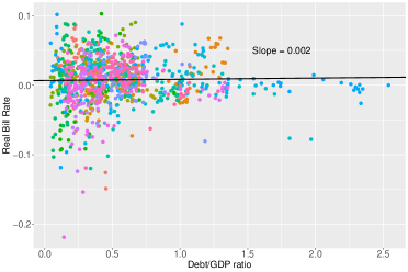
(a) Levels

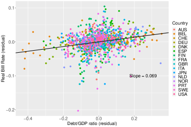
(b) Deviations from quadratic trends

Figure 1: Relationship between public debt and interest rates

Note: Data are from the MacroHistory Database (Jorda et al., 2017; Jorda et al., 2019) for the years 1950-2020.

As demonstrated by the previous analysis, government debt can be inflationary under active monetary policy if it induces demand pressure and raises the neutral interest rate. While it will become clear below that the actual realization of inflation also depends on central bank policy, a natural pre-condition for there to be any effects is that increasing public debt actually exerts upward pressure on liquid asset returns. While predicted by a range of economic theories, one might object against the existence of such effects due to empirical observations as in Figure 1(a): Using data from the MacroHistory database (Jorda et al., 2017; Jorda et al., 2019) for the period 1950-2019, it plots the real treasury bill rates of a range of developed countries against their debt-to-GDP ratios. There is no obvious correlation between the both, a simple linear regression of the former on the latter yields a slope coefficient of $\approx 0$. But of course, this overlooks that in most developed countries, rising public debt levels in more recent years were also accompanied by other secular trends that exert negative pressure on interest rates, such as demographic change or productivity growth slowdowns. In turn, 1(b) visualizes the relationship between both variables after purging them of country-specific quadratic time trends, a common way to account for long-run trends in empirical macroeconomics (cf. Ramey, 2016). We now observe a positive correlation between both variables, with a 1% deviation of a country’s debt-to-GDP ratio from trend now being associated with a 6.9 basis points (bp) higher bill rate (relative to trend). As is perhaps needless to say, the results of such a simple analysis should not be interpreted as a causal relationship and could have a range of potential explanations. However, they align well with an empirical literature attempting to measure the effects of public debt on treasury rates empirically, exemplified e.g. by Engen and Hubbard (2005) or Laubach (2009). According to a summary in Rachel and Summers (2019), such estimates range between 3 and 6 bp. Thus, reasonable values should be in a similar range, with the analysis above suggesting that slightly higher values might be justifiable.
Another body of evidence relevant for the 2-asset model is work pointing to increases in public debt raising spreads between government bonds and other assets that are less liquid (and hence less well-suited for self-insurance purposes): In particular, Krishnamurthy and Vissing-Jorgensen (2012) find that increases in the debt-to-GDP yield lower spreads between treasury returns and corporate bonds. Bayer et al. (2023a) also find rising spreads between treasuries and various less liquid assets in response to identified fiscal policy shocks that cause public debt expansions.

3 The Quantitative HANK model

While the analytically tractable model in the previous section allowed for a sharp characterization of the inflationary effects of government policy, its simplicity only allows for a qualitative assessment of the mechanism at hand. But are they likely to be quantitatively relevant? While recent empirical work has shown that fiscal expansions are indeed linked to subsequent inflation (e.g., de Soyres et al., 2022; Jordà and Nechio, 2023), such reduced-form evidence does not allow discriminating between different channels: Indeed, instead of resulting from the usefulness of government debt for insurance purposes, they could equally be due to the FTPL or a combination of the two.
In turn, I employ a quantitative model featuring only the former mechanism: In particular, I use a framework similar to Consolo and Hänsel (2023), which extends a 2-asset HANK model in the veins of Bayer et al. (forthcoming) with Search-and-Matching (SaM) frictions on the labor market. This has several attractive features: Firstly, the resulting time-varying unemployment rate creates an additional realistic source of public debt expansions in response to adverse business cycle shocks, as the government finances the temporarily higher UI expenditures by issuing debt. Secondly, the previous literature has argued time-variation in unemployment risk to be a potentially important driver of real interest rates and inflation by the literature, e.g. Ravn and Sterk (2017). This mechanism, not present in the analytical model, could potentially counteract the inflationary effects of government debt and should thus be accounted for.
A two-asset structure is important to allow the model to both include capital investment and generate empirically plausible MPCs. Additionally, it will turn out that limited suitability of capital for providing liquid assets and the resulting time-varying liquidity premia will be important for the quantitative magnitude of the results. To allow for flexibility in this regard, I introduce a financial intermediary referred to as the liquid asset fund below.
While it is always assumed that the fiscal authority is committed to eventually consolidating its debt at the initial steady state level, I will consider different policy rules for doing so in Section 5. Additionally, the central bank is always following an “active” Taylor rule, with different versions being considered in Section 7.

3.1 Period timing

In the model, time is discrete and runs forever, starting from $t=0$. Every period, there is the following order of events, on which additional details will be provided below:

1. Aggregate shocks are revealed; job separations take place; Government policies are announced

2. The labor market opens: Labor agencies post vacancies; Unemployed search for jobs; matches are formed

3. The labor market closes; there is an even number of $M$ subperiods during which production takes place and workers and labor agencies can negotiate over wages

4. Goods and asset markets open: Asset returns are paid out; consumption and investment decisions are made

5. Goods and asset markets close; shocks to idiosyncratic states $s_{it}$ and $\Xi_{it}$ are revealed

3.2 Households

3.2.1 Idiosyncratic states

There is a unit mass of households, which I again also refer to as “agents” interchangeably. These differ ex-post by several idiosyncratic states:

• First of all, households vary in terms of their holdings of liquid and illiquid assets $a_{it}$ and $k_{it}$. $k_{it}$ represents holdings of capital and we require that $k_{it}\geq 0$ as well as $a_{it}\geq\underline{a}$, with $\underline{a}$ representing an exogenous borrowing limit. Capital is illiquid in that a household can change her stock $k_{it}$ only infrequently: In particular, following Bayer et al. (forthcoming) and Auclert et al. (2023), I assume that the opportunity to do so arises randomly in an i.i.d. fashion, in that households only gets to participate in the market for illiquid assets with probability $\lambda\in(0,1)$ every period.

• Secondly, the agents can be workers ($\Xi_{it}=0$) or “entrepreneurs” ($\Xi_{it}=1$). The former participate in the frictional labor market, while the latter don’t supply labor to the market but receive the profits generated by the firms (to be described below), which, for simplicity, are assumed to be shared equally among all households with $\Xi_{it}=1$. Transitions to and out of the “entrepreneur” state are exogenous with probabilities $\zeta$ and $\iota$.

• Worker households ($\Xi_{it}=0$) additionally differ by their idiosyncratic labor productivity or “skill” $s_{it}\in\mathcal{S}=\{s_{1},s_{2},...,s_{ns}\}$, which evolves stochastically according to a discrete Markov chain. I allow for transition probabilities $\pi^{s}(s_{it+1}|s_{it},e_{it})$ to depend on employment status $e_{it}$ (see next bullet point) in order to parsimoniously capture skill accumulation (depreciation) while employed (unemployed). Workers who are selected to become entrepreneurs lose their idiosyncratic $s_{it}$ state as well as their job, while exiting entrepreneurs draw a new $s_{it}$ according to exogenous probabilities $p_{s_{1}},p_{s_{2}},...$ and enter unemployment.

• Finally, workers will either be employed $(e_{it}=1)$ or unemployed ($e_{it}=0$). I assume there to be no disutility from either work or job search, so that all workers will be working or searching full time. Job finding rates $p^{UE}_{t}$ and $p^{EU}_{t}(s_{it})$ will be endogenously determined on the frictional labor market described in Section 3.4.2. Note that the latter may depend on individual labor productivity.
  Workers receive a wage $w_{t}(s_{it})$, while unemployed agents receive an unemployment insurance (UI) benefit $b_{t}(s_{it})$. As outlined above, wages $w_{t}$ will be the outcome of an AOB bargaining protocol to be described in Appendix B.1, while $b_{t}(s_{it})$ is set by the government: its level is assumed to depend on $s_{it}$ to introduce dependence on previous income without adding additional state variables to the household problem.

Below, I will by denote by $m_{t}(\cdot)$ the mass of households that, at the beginning of a period, are currently in the specified state, e.g. $m_{t}(k,s,e)$ is the respective measure of households with capital holding $k$, skill $s$ and employment status $e$. Additionally, I will use the superscripts $e,u$ and $\Xi$ to refer to variables specific to the employed, unemployed or entrepreneurs when it does not cause confusion. For example, I will use $m^{e}_{t}$, $m^{u}_{t}$ and $m_{t}^{\Xi}$ to denote the masses of agents that feature states $e_{it}=1$, $e_{it}=0$ or $\Xi_{it}=1$ at the beginning of stage 4 of any period $t$ (compare Section 3.1 above).

3.2.2 The Household problem

Households value a consumption stream $\{c_{t}\}^{\infty}_{t=0}$ according to standard time-separable CRRA preferences

$$\mathbb{E}_{0}\sum^{\infty}_{t=0}\beta^{t}\frac{c_{it}^{1-\xi}-1}{1-\xi}~{}~{}.$$ (16)

An agent who gets to adjust her illiquid capital stock will the face budget constraint

$$c_{it}+q_{t}k_{it+1}+a_{it+1}=(1-\tau_{t}^{y})y_{it}(e_{it},s_{it},\Xi_{it})+(1+r_{t}^{a}(a_{it}))a_{it}+(q_{t}+r^{k}_{t})k_{it}$$ (17)

while for non-adjusters, the constraint will be of the form

$$c_{it}+a_{it+1}=(1-\tau_{t}^{y})y_{it}(e_{it},s_{it},\Xi_{it})+(1+r_{t}^{a}(a_{it}))a_{it}+r^{k}_{t}k_{it}~{}~{}.$$ (18)

Both budget constraint are already written in real terms. Furthermore, $\tau^{y}$ represents a proportional income tax, $q_{t}$ the time $t$ price of capital goods, $r_{t}^{k}$ the real net return of capital goods and $r_{t}^{a}(a_{it})$ the real return on bonds $a_{it}$. The latter depends on $a_{it}$ due to the presence of a borrowing penalty. In particular, we have

$$r_{t}^{a}(a_{it})=\begin{cases}r_{t}^{l}~{}~{}~{}~{}\text{if}~{}~{}a_{it}\geq 0\\ r_{t}^{l}+\bar{R}~{}~{}~{}~{}\text{if}~{}~{}a_{it}<0\end{cases}$$ (19)

where $r_{t}^{l}$ is the real return on liquid savings, which will be effectively determined by the nominal central bank rate $R_{t}^{b}$ and inflation $\pi_{t}=\frac{P_{t}}{P_{t-1}}$ as described below. $\bar{R}$ is a real borrowing penalty. Finally, $y_{it}$ represents a household’s labor-, transfer- or profit income which will be given by

$$y_{it}(e_{it},s_{it},\Xi_{it})=\begin{cases}w_{t}(s_{it})~{}~{}~{}~{}\text{if}~{}~{}e_{it}=1,~{}\Xi_{it}=0\\ b_{t}(s_{it})~{}~{}~{}~{}\text{if}~{}~{}e_{it}=0,~{}\Xi_{it}=0\\ \frac{\Pi_{t}}{m_{t}^{\Xi}}~{}~{}~{}~{}\text{if}~{}~{}\Xi_{it}=1\\ \end{cases}~{}~{}.$$ (20)

This formulation implies that unemployment benefits are subject to taxation, as they indeed are in the US. Note that since the model does not feature an intensive labor supply margin, the introduction of tax progressivity would not have any related effects but be purely redistributive.
Letting $\Gamma_{t}$ denote a set containing the economy’s aggregate state at period $t$, we are now ready to state the Bellman equation corresponding to the households’ dynamic utility maximization problem, which are

$$V^{a}(a_{it},k_{it},e_{it},s_{it},\Xi_{it};\Gamma_{t}) =\max_{c_{it},k_{it+1},a_{it+1}}\left\{\frac{c_{it}^{1-\xi}-1}{1-\xi}+\beta\mathbb{E}_{t}V(a_{it+1},k_{it+1},e_{it+1},s_{it+1},\Xi_{it+1};\Gamma_{t+1})\right\}$$

s.t. to (17), (20), $$k_{it}\geq 0 a_{it}\geq\underline{a}$$ and (21)

for an household able to adjust its capital stock and

$$V^{na}(a_{it},k_{it},e_{it},s_{it},\Xi_{it};\Gamma_{t}) =\max_{c_{it},a_{it+1}}\left\{\frac{c_{it}^{1-\xi}-1}{1-\xi}+\beta\mathbb{E}_{t}V(a_{it+1},k_{it},e_{it+1},s_{it+1},\Xi_{it+1};\Gamma_{t+1})\right\}$$

s.t. to (18), (20), $$k_{it}\geq 0 a_{it}\geq\underline{a}$$ and (22)

for an household that unable to do so. The ex-ante value function $V(\cdot)$ is given by

$$V(a_{it+1},k_{it},e_{it+1},s_{it+1},\Xi_{it+1};\Gamma_{t+1}) =\lambda V^{a}(a_{it},k_{it},e_{it},s_{it},\Xi_{it};\Gamma_{t})$$

$$+(1-\lambda)V^{na}(a_{it},k_{it},e_{it},s_{it},\Xi_{it};\Gamma_{t})~{}~{}.$$

3.3 Production

The model’s supply side is similar to standard “medium scale” DSGE models, except the way the labor market is modelled: Production is vertically integrated. There is again a final good, that can either be consumed or used by capital goods producers to produce investment goods subject to adjustment costs. This final good is assembled by a representative final goods producer, that in turn requires differentiated inputs provided by a continuum of retailers. The latter set prices in a monopolistic competitive fashion subject to nominal rigidities and require intermediate goods to produce their output. These are provided by a set of competitive intermediate goods producers that require capital and labor services as inputs. However, the production of the labor input requires hiring on a frictional labor market à la Diamond-Mortensen-Pissarides, which is handled by labor agencies.
As Bayer et al. (forthcoming), I make the simplifying assumption that entrepreneurs don’t make the dynamic decisions of the various firms directly but instead outsource them to a group of risk-neutral managers with aggregate measure $0$, which do not have access to asset markets and discount the future at the same rate $\beta$ as the households.

3.3.1 Final goods production

The problem of the final goods producer is equivalent to the one described in Section 2.1.2 and thus omitted. For notational convenience below, I define $\mu:=\frac{\epsilon}{\epsilon-1}$.

3.3.2 Retailers

There is a unit mass of retailers, each of which produce a given variety of the differentiated input as monopolist, taking into account demand schedule (4). Their only input are intermediate goods, which they purchase at real price $mc_{t}$ (also referred to as “marginal costs”) from the competitive intermediate goods producers. However, they are subject to nominal rigidities à la Calvo (1983) with price indexation, i.e. they can only re-set their price if chosen with an exogenous probability $\lambda_{Y}$.
If not receiving the re-set opportunity, a retailer’s price is automatically adjusted by the steady inflation rate $\pi_{SS}$. If receiving it, the retailer will choose a price to maximize the corresponding expected net present value of real profits

$$\mathbb{E}_{0}\sum^{\infty}_{t=0}\beta^{t}(1-\lambda_{Y})^{t}\left(\frac{p^{*}_{jt}\pi_{SS}^{t}}{P_{t}}-mc_{t}\right)\left(\frac{p^{*}_{jt}\pi_{SS}^{t}}{P_{t}}\right)^{\frac{-\mu}{\mu-1}}Y_{t}~{}~{}.$$

Log-linearizing the first order conditions of the resulting price setting problem gives rise to the standard log-linear Phillips curve

$$\log\left(\frac{\pi_{t}}{\pi_{SS}}\right)=\kappa_{Y}\left(mc_{t}-\frac{1}{\mu}\right)+\beta\mathbb{E}_{t}\log\left(\frac{\pi_{t+1}}{\pi_{SS}}\right)$$ (23)

with $\kappa_{Y}:=\frac{(1-\lambda_{Y})(1-\lambda_{Y}\beta)}{\lambda_{Y}}$.

3.3.3 Intermediate goods producers

The homogeneous intermediate good is produced by a continuum of firms that use a constant-returns-to-scale technology represented by production function

$$F_{t}(u_{t}K_{t},H_{t})=Z_{t}F(u_{t}K_{t},H_{t})=Z_{t}(u_{t}K_{t})^{\alpha}H_{t}^{1-\alpha}~{}~{}.$$ (24)

$K_{t}$ and $H_{t}$ denote the input of capital and labor services. $u_{t}$ is the degree of capital utilization that determines capital depreciation according to

$$\delta(u_{t})=\delta_{0}+\delta_{1}(u_{t}-1)+\frac{\delta_{2}}{2}(u_{t}-1)^{2}~{}~{}$$

and $Z_{t}$ is a shock to Total Factor Productivity (TFP). Taking the price $h_{t}$ for labor services as well as the capital rental rate $r_{t}$ and its output price $mc_{t}$ as given, an intermediate goods producer solves the static profit maximization problem

$$\max_{K_{t},H_{t},u_{t}}mc_{t}F_{t}(u_{t}K_{t},H_{t})-h_{t}H_{t}-(r_{t}+q_{t}\delta(u_{t}))K_{t}~{}~{},$$

the solution of which can be characterized using the following first order conditions:

$$h_{t} =(1-\alpha)mc_{t}Z_{t}(u_{t}K_{t})^{\alpha}H_{t}^{-\alpha}$$ (25)

$$r_{t}+q_{t}\delta(u_{t}) =\alpha mc_{t}Z_{t}u_{t}(u_{t}K_{t})^{\alpha-1}H_{t}^{1-\alpha}$$ (26)

$$q_{t}(\delta_{1}+\delta_{2}(u_{t}-1)) =\alpha mc_{t}Z_{t}(u_{t}K_{t})^{\alpha-1}H_{t}^{1-\alpha}~{}~{}.$$ (27)

3.3.4 Capital goods producer

Capital goods producers use the final good as input and operate a technology subject to adjustment costs: Using $I_{t}$ units of the final good, they can produce

$$\left[1-\frac{\phi}{2}\left(\frac{I_{t}}{I_{t-1}}-1\right)^{2}\right]I_{t}$$

units of capital.
Taking the price of capital $q_{t}$ as given, the producers choose $I_{t}$ to maximize the net present value of real profits

$$\mathbb{E}_{0}\sum^{\infty}_{t=0}\beta_{t}\left(q_{t}\left[1-\frac{\phi}{2}\left(\frac{I_{t}}{I_{t-1}}-1\right)^{2}\right]I_{t}-I_{t}\right)~{}~{}$$

and their optimal interior solution will fulfill first-order condition

$$q_{t}\left(\frac{\phi}{2}\left(\frac{I_{t}}{I_{t-1}}-1\right)^{2}+\phi\left(\frac{I_{t}}{I_{t-1}}-1\right)\frac{I_{t}}{I_{t-1}}\right)=\beta q_{t+1}\phi\left(\frac{I_{t+1}}{I_{t}}-1\right)\left(\frac{I_{t+1}}{I_{t}}\right)^{2}.$$ (28)

3.4 Labor market

3.4.1 Labor agencies

Labor services are produced by a continuum of homogeneous labor agencies, each of which is matched with at most one worker of productivity $s$. Such a match produces $s_{t}$ units of the labor service output, the price of which are taken as given by an agency. Job separations are exogenous and take place either if (1) the match is subject to an separation shock arriving with probability $\delta(s)$ or if (2) the worker becomes an entrepreneur with probability $\zeta$. I allow for job separation rates $\delta(s)$ to depend on skill, consistent with evidence that low-income workers face higher job separation risk (see e.g. Birinci and See, 2021). Given all the above, the recursive characterization of the value of a matched agency is

$$J(s_{t};\Gamma_{t})=h_{t}s_{t}-w_{t}(s_{t})+(1-\zeta)(1-\delta(s_{t}))\beta\mathbb{E}_{t}J(s_{t+1};\Gamma_{t+1})~{}~{}.$$ (29)

3.4.2 Job matching and vacancy creation

There is a single labor market, on which unmatched labor agencies can meet unemployed workers by posting vacancies. The number of meetings is governed by a Cobb-Douglas matching technology

$$M_{t}(V_{t},U_{t})=A_{m}U_{t}^{\chi}V_{t}^{1-\chi}~{}~{}.$$ (30)

$V_{t}$ represents the total number of vacancies posted and

$$U_{t}=m_{t}(e=0)+\sum_{s_{i}\in\mathcal{S}}\delta(s_{i})m_{t}(e=1,s=s_{i})$$

the total mass of workers searching for a job. From (30), it follows that the period-$t$ job-finding probability $p^{UE}_{t}$ and vacancy-filling probability $p^{vf}_{t}$ are

$$p^{UE}_{t}=\frac{M_{t}(V_{t},U_{t})}{U_{t}}=A_{m}\theta_{t}^{1-\chi}~{}~{}~{}\text{and}~{}~{}~{}p^{vf}_{t}=\frac{M_{t}(V_{t},U_{t})}{V_{t}}=A_{m}\theta_{t}^{-\chi}~{}~{},$$ (31)

respectively. $\theta:=V_{t}/U_{t}$ is the labor market tightness.
Hiring is costly in that posting a vacancy incurs a real resource cost of $\kappa$. Labor market tightness is in turn pinned down by a free entry condition of the form

$$\kappa=p_{t}^{vf}\left(\sum_{s\in\mathcal{S}}\frac{U_{t}(s)}{U_{t}}J(s;\Gamma_{t})\right)$$ (32)

with

$$U_{t}(s_{i})=m_{t}(e=0,s=s_{i})+\delta(s_{i})m_{t}(e=1,s=s_{i})$$

denoting the mass of job-searchers of a given skill level $s_{i}\in\mathcal{S}$. These terms are present because labor agencies take into account which type of workers they are most likely to meet.

3.4.3 Wage determination

Wages are determined according to an intra-period Alternative Offer Bargaining (AOB) protocol in the veins of Christiano et al. (2016), imposing the restriction of no intra-period bargaining break-downs used by Ljungqvist and Sargent (2021): As shown by Consolo and Hänsel (2023), such a setting avoids the dependence of wages on the asset positions of individual workers resulting from other bargaining protocols such as Nash bargaining.
The wages resulting from the protocol are given by

$$w_{t}(s)=\frac{1}{2}\left(h_{t}s+\tilde{b}_{t}(s)\right)+\frac{M-2}{2M}\gamma(s)+(1-\zeta)(1-\delta(s_{t}))\beta\mathbb{E}_{t}J(s_{t+1},\Gamma_{t})~{}~{},$$ (33)

with $\tilde{b}_{t}(s)$ denoting an outside income that a worker of skill $s$ receives while in disagreement with its employer. More details on the AOB bargaining protocol as well as the derivation of (33) are provided in Appendix B.1.

3.5 Liquid Asset Provision

While I assume a centralized market for claims to (illiquid) capital, households obtain liquid assets from a set of competitive liquid asset funds (LAFs). In contrast to households, these funds are able to trade claims to capital every period and also have access to a technology to short-sell them. Their objective is to maximize expected returns by investing the funds $A_{t+1}^{l}$ received from the households in capital and government bonds. In particular, the LAFs solve

$$\max_{B^{l}_{t+1}}\left\{\mathbb{E}_{t}\left[(r_{t+1}^{k}+q_{t+1})\frac{A_{t+1}^{l}-B_{t}^{l}}{q_{t}}+\frac{R^{B}_{t+1}}{\pi_{t+1}}B^{l}_{t+1}\right]-A_{t+1}^{l}\left(\varphi+\frac{\Psi}{2}\left(1-\frac{B_{t+1}^{l}}{A_{t+1}^{l}}\right)^{2}\right)\right\}~{}~{}~{},$$ (34)

where $A_{t+1}^{l}$ denotes the total amount of assets intermediated by the LAF and $B_{t}^{l}$ the amount of government debt it chooses to acquire. A fund faces costs for each unit of liquid asset it invests on behalf of the households, which involve the linear component $\varphi$ and a part $\frac{\Psi}{2}\left(1-\frac{B_{t}^{l}}{A_{t}^{l}}\right)^{2}$ that increases in the relative amount of assets the fund does not invest in public debt obligations. Its portfolio choice can be determined from the corresponding F.O.C.

$$\mathbb{E}_{t}\left(\frac{r^{k}_{t+1}-q_{t+1}}{q_{t}}\right)-\Psi\left(1-\frac{B_{t+1}^{l}}{A_{t+1}^{l}}\right)=\mathbb{E}_{t}\left(\frac{R^{B}_{t+1}}{\pi_{t+1}}\right)$$ (35)

and the ex-post return to household’s liquid savings will be given by

$$r_{t}^{l}=\frac{(q_{t}+r_{t}^{k})(A_{t}^{l}-B_{t}^{l})+\frac{R^{B}_{t}}{\pi_{t}}B^{l}_{t}}{A_{t}^{l}}-\varphi-\frac{\Psi}{2}\left(1-\frac{B_{t}^{l}}{A_{t}^{l}}\right)^{2}-1~{}~{}.$$ (36)

A few words on the above structure are in order: The aim of the perhaps peculiar cost structure in (70) is not to provide a particularly realistic model of financial intermediation, but rather to introduce a parsimonious way to flexibly move between various assumption on liquid asset supply in the literature. For this purpose, the parameter $\Psi$ has a simple interpretation as determining how easily capital assets can be used for liquidity provision: For $\Psi\rightarrow\infty$, the model nests the assumption of segmented markets for liquid and illiquid assets as in Kaplan et al. (2018) or Bayer et al. (forthcoming); for $\Psi\rightarrow 0$ it nests a completely integrated market as in Auclert et al. (2023). While a micro-founded model of financial intermediation as e.g. in Dominguez Diaz (2021) could also provide for imperfect usefulness of capital for liquidity provision, it would be less straightforward to map into the above limit cases and potentially harder to interpret.

3.6 Government

The government again consists of two branches, a monetary authority and a fiscal authority.

3.6.1 Monetary Authority

The monetary authority sets the nominal interest rate on government bonds, which follow a Taylor rule of the form

$$\frac{R_{t+1}^{B}}{R^{B}_{SS}}=\left(\frac{R_{t}^{B}}{R^{B}_{SS}}\right)^{\rho^{B}}\left[\left(\frac{\pi_{t}}{\pi_{SS}}\right)^{\theta_{\pi}}\exp(m_{t}^{u}-m^{u}_{SS})^{-\theta_{u}}\right]^{1-\rho^{B}}~{}~{}.$$ (37)

The parameter $\rho^{B}$ introduces rate smoothing and if $\theta_{u}\neq 0$, the rule reacts to unemployment in addition to inflation.

3.6.2 Fiscal Authority

The fiscal authority collects taxes, pays out unemployment insurance and engages in government consumption $G_{t}$. Its budget constraint (in real terms) is

$$B^{g}_{t+1}+\tau_{t}^{y}\left(\sum_{s\in\mathcal{S}}w_{t}(s)m^{e}_{t}(s)+\Pi_{t}\right)=G_{t}+\frac{R^{B}_{t}}{\pi_{t}}B^{g}_{t}+\sum_{s\in\mathcal{S}}(1-\tau^{y}_{t})b_{t}(s)m^{u}_{t}(s)~{}~{}.$$ (38)

For simplicity, I assume the value of UI benefits to be equal to a fixed fraction of real steady wages, i.e.

$$b_{t}(s)=\Upsilon_{b}w_{ss}(s)~{}~{}.$$ (39)

Furthermore, in the baseline model I assume government consumption $G_{t}$ to remain constant at its Steady State level $G_{ss}$ and taxes to follow the rule

$$\left(\frac{\tau^{y}_{t}}{\tau^{y}_{s}s}\right)=\left(\frac{\tau^{y}_{t-1}}{\tau^{y}_{ss}}\right)^{\rho_{\tau}}\left(\frac{B^{g}_{t}}{B^{g}_{ss}}\right)^{(1-\rho_{\tau})\psi_{B}},$$ (40)

with the fiscal authority to issue any amount of bonds $B^{g}_{t+1}$ necessary to fulfill its budget constraint (38). Intuitively, policy (40) means that the government will eventually raise taxes to pay back debt in surplus of its long-run target, but may do so only slowly. In Appendix C.1, I will consider the alternative scenario in which the fiscal authority consolidates its budget by adjusting spending $G$ instead of taxes $\tau_{y}$. Furthermore, in the baseline model, all government debt is short-term, i.e. consists of 1-period bonds. Appendix C.2 will also discuss a version of the model in which the fiscal authority issues long-term debt obligations. This affects some model dynamics, but does not alter the main insights.

3.7 Market clearing conditions and equilibrium

The Definition of Equilibrium is standard, but tedious, given that the quantitative model features multiple markets and also requires keeping track of the evolution of measures $m_{t}(\cdot)$. In turn, I relegate these details to Appendix B.2.

3.8 Numerical Approach

I approximate the dynamic equilibrium of the model using a version of the method used by Bayer and Luetticke (2020), which conducts first-order perturbation around the economy’s non-stochastic steady state, following a dimension reduction step.
For obtaining that steady state, I use a multidimensional Endogenous Grid Method similar to the algorithm described in Bayer et al. (2019) to solve the households’ dynamic programming problem. The joint income- and asset distribution is approximated as a histogram using the “lottery”-method proposed by Young (2010).
However, the representations of the (marginal) value functions as well as the joint distribution on a tensor grid are too large to be practically handled by standard perturbation algorithms. In turn, the dimensionality of the (marginal) value function is reduced by applying a Discrete Cosine Transform (DCT) and perturbing only the coefficients most important for the shape of the steady state marginal value function. Additionally, the joint distribution is split into a copula and marginals and I only perturb the marginals as well as the largest coefficients resulting from a similar DCT of the copula.
Further details on the numerical implementation are provided in Appendix B.4.

3.9 RANK/TANK versions

To gain further insights on how idiosyncratic income risk and high MPCs matter for the effects of government debt on inflation, it is useful to compare the results of the full-blown HANK economy with those of similar New Keynesian models featuring only a representative agent (also called RANK models) or Two Agents (so-called TANK models). In the former, Ricardian equivalence holds and the household’s MPC is very low. The latter breaks Ricardian equivalence by introducing a group of “constrained” agents unable to participate in asset markets, which also results in high average MPCs. However, it still does not feature any idiosyncratic income risk and will thus not provide for medium- to long run effects of government debt on real interest rates.
I construct these alternative frameworks to resemble the baseline HANK economy as close as possible. In particular, all frameworks will feature the same parameters except for $\beta$ and $R^{B}_{SS}$: In RANK and TANK, the agents with asset market access can overcome the illiquid asset adjustment friction by trading state-contingent securities, so that a no-arbitrage condition between government bonds and capital will have to hold. In turn, I always choose $\beta$ and $R^{b}_{SS}$ to be consistent with the same steady state return on capital as in the HANK economy.

4 Calibration of the quantitative model

A model period is interpreted to be a quarter. I aim for the model to be consistent with the most relevant features of the US economy and first set a range of parameters exogenously, relying on the previous literature: In addition to standard preference- and technology parameters, this includes some parameters exclusively affecting the dynamic model response to aggregate shocks, for which I rely on previous papers estimating a HANK model. Afterwards, the remaining parameter values are chosen to match various steady state distribution- and labor market moments.

4.1 Externally calibrated

Parameter	Description	Value	Source
$\xi$	risk aversion	1.0	Standard
$\iota$	Exit prob. entrepreneurs	1/16	Bayer et al. (forthcoming)
$\alpha$	Cobb-Douglas parameter	0.32	Standard
$\delta_{0}$	Steady State depreciation	0.015	Standard
$\mu$	SS Goods markup	1.1	Standard
$\kappa_{Y}$	Slope of Phillips curve	0.08	Standard
$\phi$	investment adjustment cost	3.5	Bayer et al. (forthcoming)
$\delta_{2}/\delta_{1}$	utilization parameters	1.0	Bayer et al. (forthcoming)
$\chi$	matching elasticity	0.5	Petrongolo and Pissarides (2001)
$M$	no. bargaining periods	60	Christiano et al. (2016)
$(\rho_{\tau},\psi_{B})$	Gov’t spending rule	(0.94, 0.35)	Bayer et al. (2023b)
$\tau^{y}$	Proportional income taxes	$0.25$	See text
$\Upsilon_{b}$	SS UI replacement rate	0.4	Shimer (2005)
$(\rho_{R},\theta_{\pi},\theta_{u})$	Taylor rule parameters	(0.75,1.5,0.0)	Standard
$\pi_{ss}$	Inflation Target	1.0	Standard

Table 1: Externally set parameters

The household’s risk aversion parameter is set to $1.0$, a standard value in the macroeconomic literature also used by Kaplan et al. (2018). Regarding technology, I use the standard values of $\alpha=0.32$ for the Cobb-Douglas parameter for capital and set a quarterly depreciation rate for capital of $\delta=0.015$, implying approx. 6% annual depreciation. Similar, I set $\mu_{t}$ to a conventional value of $1.1$, resulting in a steady state markup of 10%. The number of subperiods during which bargaining can take place is $M=60$, the same value as in Christiano et al. (2016): this reflects the typical number of business days within a quarter. I furthermore set $\chi=0.5$, a standard value for the matching elasticity going back to by Petrongolo and Pissarides (2001).
Several other parameters governing the economy are calibrated following Bayer et al. (forthcoming): First, I also set the probability of exiting the $\Xi=1$ state within a given period to be $6.25$%. The investment adjustment cost is chosen to be $3.5$ and the ratio $\delta_{2}/\delta_{1}$ set to be $1$, reflecting the results of their model estimation. For a given $\delta_{2}/\delta_{1}$-ratio, I always set $\delta_{1}$ and $\delta_{2}$ to achieve $u_{t}=1.0$ in steady state.
The government policies are parameterized as follows: I proceed as Shimer (2005) by choosing an unemployment replacement rate of $0.4$. As is standard, the central bank is assumed to target zero net inflation, i.e. $\pi_{ss}=1$, and chooses $R^{b}_{SS}$ so that this is achieved in the economy’s non-stochastic steady state. Regarding the interest rate rule, the baseline calibration employs the standard value of $\theta_{\pi}=1.5$ and features some nominal rate persistence with $\rho_{R}=0.75$. Since it is not crucial for assessing the inflationary effects of public debt, I abstract from an unemployment reaction in main text but consider a robustness exercise below. Other parameterizations of the rule are also considered in Section 7. Next, I assume all proportional income taxes to equal 25%: These values are close both to the average US tax rates on labor incomes as well as profits and are consistent with a reasonable long-run government consumption-to-GDP ratio of $G/Y=0.158$. Finally, the policy rule for taxes is assumed to feature substantial persistence with $\rho_{\tau}=0.94$ and $\psi_{B}=0.35$: Since assessing the inflationary effects of government debt requires inducing different time paths of it, this rule will naturally be contrasted with other scenarios below.

4.2 Internal calibration

Parameter	Description	Value	Target
$\beta$	Time discounting	$0.9838$	$K/Y=11.44$
$\zeta$	prob. entrepreneur state	0.0003	Wealth share top 10
$\lambda$	prob. illiquid asset adjustment	$0.0901$	$A^{l}/Y=1.04$
$\bar{R}$	Borrowing penalty	0.0449	16% borrower share
$B_{ss}$	Government debt	1.9269	$B_{ss}=A^{l}_{ss}$
$G_{ss}$	Government consumption	$0.2915$	Budget clearing (38)
$\varphi$	Liquidity Cost	0.0103	$r^{l}_{ss}=0$
$\Psi$	Liquidity Supply	0.005	See text
$\underline{a}$	Borrowing limit	-0.873	100 % avg. quart. income
$A_{m}$	Matching efficiency	0.6522	Unemployment rate $5.5\%$
$\kappa$	vacancy cost	0.0473	7% of avg. hire wage
$s$	Individual labor productivity	See Appendix B.5	See text
$\gamma(s)$	Costs of delay	See Appendix B.5	See text
$\delta(s)$	Separation rates	See Appendix B.5	See text

Table 2: Internally calibrated parameters

The remaining parameters are chosen so that the model matches various target moments in the non-stochastic steady state. To clarify how they come about, I present for each parameter the moment I use to identify it. While, if taking other parameters as given, any parameter will somewhat affect any of the stationary equilibrium’s target moments, it is often the case that if one assumes other target moments to have been realized, individual parameters can be identified just by the respective moments. For the parameters for which this is not true, it nevertheless turns out that achieving a good fit with the target relies mostly on the stated parameter.
Several parameters are disciplined by moments related to the steady state wealth distribution. I choose the household discount factor $\beta$ to match a ratio of average steady state capital holdings to output of $11.44$ as in Bayer et al. (2019), resulting in $\beta=0.9838$. $\lambda$ determines the (il-)liquidity of capital and thus how much liquid bonds agents wish to additionally hold for self-insurance purposes: I use it to target net liquid asset holdings by households to equal 1.04 times quarterly GDP as in Kaplan et al. (2018). This requires $\lambda=0.0901$. The borrowing penalty $\bar{R}$ determines the share of households with a negative liquid asset position: to get a share of 16%, I set value of $0.0449$. The probability $\zeta$ determines the amount of “super rich” entrepreneur households and I use it to target a Top 10% wealth share of 70%, approximately the value computed by Krueger et al. (2016) using SCF data. This requires a value of approx. $0.0003$. Additionally, I set the value of the borrowing constraint to the equal average quarterly steady state labor- and transfer income, in line with Kaplan et al. (2018).
In order to be able to flexibly consider different values for $\Psi$, I require all liquid assets held by households in Steady State to be provided by the government, i.e. $B_{ss}=A^{l}_{ss}$. While a Steady State Government Debt to (annual) GDP ratio of $26\%$ may seem low for the US, it actually corresponds well to the corresponding ratio for the federal debt held by the public minus the debt held by foreign and international investors. In particular, for the period 1970-2019, the ratio of Federal Debt held by the domestic public to annual GDP was 28.6%, which is arguably the relevant ratio for a closed economy model. Next, I set $\phi=0.0103$ which will induce the Steady State liquid return $r_{t}^{l}$ to equal $0$ as in Bayer et al. (forthcoming). The calibration of $\Psi$ is detailed in 4.3. $G_{ss}$ is eventually set as the value fulfilling (38) given the other targets.
I choose matching productivity $A_{m}=0.6522$ to achieve an average unemployment rate of $5.5\%$. Furthermore, following Christiano et al. (2016), I target steady state hiring costs $\kappa/p^{vf}_{SS}$ to be 7% of the average wage of newly hired workers. This results in a vacancy posting cost of 0.0473. As them, I will also assume that a worker’s outside income during bargaining is assumed to equal her unemployment benefit. Finally, it is necessary to set the parameters connected to the individual labor productivity levels $s$. To calibrate the values for $s$ and $\gamma(s)$, I build on the literature estimating income processes: In particular, the recent paper by Braxton et al. (2021) estimates a process in which the permanent component $z_{i,t}$ of log individual income has an AR(1) form with labor market status-specific parameters

$$z_{i,t+1}=\mu_{z}(e_{it})+\rho_{z}z_{i,t}+\sigma_{z}(z_{i,t})\varepsilon_{i,t}~{}~{},$$

i.e. the drift and the innovation variance depend on whether an individual works or not. Braxton et al. (2021) argue that such a set-up captures on-the-job skill accumulation as well as human capital depreciation during unemployment. In turn, I use their annual estimates $\rho_{z}=0.94$, $(\mu_{z}(1),\mu_{z}(0))=(0.0038,-0.1472)$ as well as $(\sigma_{z}(1),\sigma_{z}(0))=(0.2261,0.4171)$, transform them into quarterly values and discretize the process onto a grid of 13 points following the methodology outlined in their paper..
This, however, provides us only with a discretized process for household’s labor earnings, i.e. the wages $w_{t}(s_{it})$, while the calibration requires the primitives determining them. Conveniently, the linearity of bargaining outcome (33) provides an easy way of backing them out: To reduce the number of parameters, I first restrict $\gamma(s)=\bar{\gamma}h_{ss}s$, i.e. that a labor agency’s costs of delay are proportionally to the revenue generated by the match in steady state. Then, together with a linear rule relating the level of worker outside income $\tilde{b}_{t}(s)=\tilde{\Upsilon}_{b}(s)w_{ss}(s)$ to the steady state wage level, the steady state match revenue $h_{ss}s$ necessary to induce the wage levels $w_{t}(s_{it})$ can be found by solving a linear system. I choose $\bar{\gamma}$ by targeting a steady state vacancy filling rate of $p^{vf}_{SS}=0.71$ (as in den Haan et al., 2000) and the $s$ levels themselves are subsequently obtained by using that other target moments provide the steady state level $h_{ss}$. The resulting values for $s$ and $\gamma(s)$ are reported in Appendix B.5.
Finally, for the separation rates $\delta(s)$, I follow Birinci and See (2021) by using the functional form $\delta(s)=\bar{\delta}\exp(\eta_{s}(s-1))$ and choosing $\bar{\delta}$ to target an average quarterly EU flow rate of $\bar{p}^{EU}_{SS}=3.5\%$ and an EU flow rate ratio of $p^{EU}(s_{ns})/p^{EU}(s_{1})=0.2$. i.e. the most productive workers are 5 times less likely to loose their jobs than the least productive ones.

4.3 Calibrating Liquidity Supply

The “fiscal inflation” mechanism explained in Section 2 depended on higher public debt stimulating demand or, vice versa, exerting upward pressure on the real (liquid asset) interest rate. Thus, for obtaining reasonable quantitative results, it will be important to ensure that this will be of a reasonable magnitude. A natural candidate to discipline this aspect of the model is to ensure consistency with the empirical evidence summarized in Section 2.5, i.e. that in the medium- to long run a 1 percentage point (p.p.) increase of the economy’s annual debt-to-gdp ratio is associated with an increase of the annual real treasury rate of roughly 3-7 bp, allowing for some leeway due to the uncertainty surrounding the various estimates.

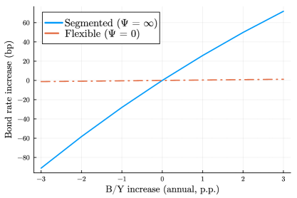
Figure 2: Model long-run effects of gov’t debt on bond returns

Can the 2-asset HANK generate a relationship of this magnitude under the limit assumptions from the literature, i.e. either $\Psi\rightarrow\infty$ or $\Psi\rightarrow 0$? Computing new steady states for different Debt-to-GDP ratios under the parameterization specified in Section 4 yields Figure 2. The results are rather stark: Under segmented asset markets, a 1 p.p. higher annual Debt-to-GDP ratio causes the annual steady state real treasury rate to increase by more 20 bp, approx. 3 times more than the upper end of the empirical estimates. The opposite is true of the integrated ($\Psi\rightarrow 0$) asset markets, in which the response of the rate is much smaller and hardly noticeable, not even a third of the empirical estimates. These findings can be rationalized as follows: In the model, households hold liquid assets only to the extent necessary to insure their idiosyncratic risk, as illiquid capital yields superior returns. Additionally, constrained households will hardly adjust their savings in response to small rate changes. Thus, if the private sector is to hold more liquid government bonds, substantial rate increases are necessary. In contrast, if liquid assets can alternatively be held in illiquid form at the same return as capital, the increase in the debt-to-GDP ratio will only crowd out a bit of the much larger capital stock, resulting in small changes of the equilibrium interest rate. We have thus to conclude that the assumption of either perfectly segmented or flexible asset markets, although attractive due to their simplicity, fail to generate a reasonable long-run relationship between government debt supply and real treasury rates.
However, we can still obtain a reasonable long-run real interest rate if we allow for a restricted usefulness of capital for liquidity provision as determined by $\Psi$. Computing new steady states for different values, we obtain Figure 3, which displays by how much a 1 p.p. higher annual Debt-to-GDP ratio increases the treasury rate compared to the original steady state.

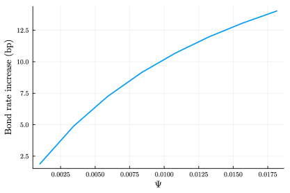
Figure 3: Increase SS treasury rate after 1 p.p. annual $B/Y$ increase

For a $\Psi$ in the range between $0.002$ and $0.007$, we obtain a difference roughly in line with the empirical results roughly in line with the empirical results summarized in Section 2.5. I choose $\Psi=0.005$ as the baseline which implies a long-run response of 6 bp, close to my own estimate. Naturally, I will consider the impact of different values below.

4.4 Distributional Moments

In this section, I validate the internal calibration by analyzing various model-generated moments that were not directly targeted.
Table 3 compares various untargeted moments of the model’s Steady State income- and wealth distributions with their empirical counterparts as reported by Krueger et al. (2016). The latter are based on the 2006 Panel Survey of Income Dynamics (PSID) and the 2007 Survey of Consumer Finance (SCF), respectively. Overall, the model achieves a fairly good fit, in particular for Net Worth. Using the “entrepreneur” status to target the Top 10 wealth share results in the model featuring somewhat higher income inequality.
Since I am employing a two-asset model, it is not only relevant to assess how closely the framework matches data moments related to the distribution of overall net worth, but also the different asset classes held by the households. I do so in Table 4: First, I am considering moments of the illiquid- and liquid wealth distribution separately. In particular, I compare them with statistics reported by Kaplan et al. (2018), who rely on the 2004 SCF. As in the data, the model generates a more unequal distribution of liquid assets and ownership of both asset classes is concentrated in their respective Top 10%, with the bottom 50% holding hardly any. Also, the model moments of the illiquid asset distribution are close to the data, mildly under-predicting the share of the Top 10%. However, for liquid assets, I generate a comparably more equal asset distributions, with the share held by the Top 10% not as high and the share of the Next 40% substantially larger than in the SCF data. But, as noted by Kaplan et al. (2018), it is “notoriously challenging” to match the extreme right tail of wealth distributions with income risk alone. From that perspective, I view my model’s performance as satisfactory.

	Disposable Income		Net Worth
	Model	Data	Model	Data
Quint. 1	4.6	4.5	0.0	-0.2
Quint. 1	8.6	9.9	1.6	1.2
Quint. 3	13.4	15.3	4.7	4.6
Quint. 4	20.8	22.8	12.0	11.9
Quint. 5	52.7	47.5	81.4	82.5
Gini	0.48	0.42	0.79	0.78

• Note: “Data” refers to moments computed by Krueger et al. (2016) using PSID and SCF.

Table 3: Distributional moments comparison

Moments	Model	Data (incl. source)
Illiquid asset shares		(from Kaplan et al., 2018)
Top 10%	65.5	70
Next 40%	31.5	27
Bottom 50%	3.0	3
Liquid asset shares		(from Kaplan et al., 2018)
Top 10%	75.5	86
Next 40%	23.5	18
Bottom 50%	1.0	-4
Hand-to-Mouth (HtM) Status		(from Kaplan et al., 2014)
Share HtM	30.5	31.2
Share Wealthy HtM	21.0	19.2
Share Poor HtM	9.5	12.1

Table 4: Portfolio moments comparison

Finally, I analyze how many households are Hand-to-Mouth (HtM) in the sense of Kaplan et al. (2014), i.e. whether their liquid asset holdings are less than 2 weeks ($\approx$ 1/6 of a model period) of current household income above of either $0$ or the borrowing constraint. I also classify them as “Wealthy HtM” if they additionally hold illiquid assets and “Poor HtM” if they do not. The model matches the empirical evidence on the size of either group of agents well. As visualized in Figure 4, these low liquid-wealth agents tend to have particularly high MPCs. In turn, my framework is able to generate an average quarterly MPC of 15.7% and an average annualized MPC of 39%. The former is of a similar magnitude as the corresponding value in Kaplan et al. (2018).

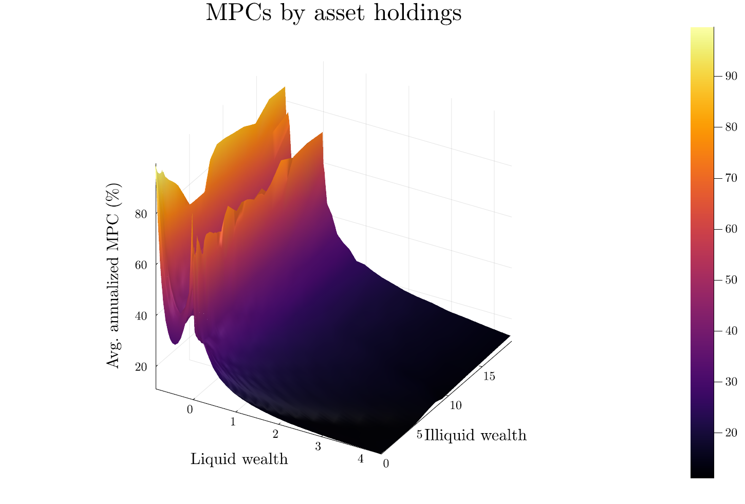
Figure 4: Model MPC distribution

4.5 Calibration for RANK/TANK

As already indicated above, I use the same parameters for the RANK/TANK versions of the model wherever possible. Thus, I only re-calibrate $\beta$ and $R^{B}_{SS}$: To be consistent with the same steady state return on capital as in the HANK economy, I set $R^{b}_{SS}=1+r^{k}_{ss}$ as implied by the $K/Y$-target and $\beta=1/R^{b}_{SS}$. Additionally, for the TANK economy, it is necessary to specify the fraction of “spender” households that are unable to participate in asset markets. Following Debortoli and Galí (2017), I assume it to be 20%. Note that since all “spenders” have an instantaneous MPC of 1, the quarterly MPC of the TANK model actually exceeds the corresponding value for the baseline HANK model.

5 Inflation after Supply Shocks

We can now use the calibrated 2-asset HANK model to study whether the time path of fiscal policy and government debt affects inflation dynamics in response to different shocks. I start doing so in the context of an inflationary supply shock, in particular a 1% decrease of TFP $Z$, which reverts to its steady state value according to an AR(1)-process in logs with persistence $0.9$. Studying such a simple scenario has both pragmatic and expositional motivations: While Federal Reserve chairman Powell (2022) concluded that “you couldn’t get this kind of inflation without a change on the supply side”, matching recent inflation dynamics is typically found to require a combination of different shocks as well as allowing for non-linear model dynamics (cf. Amiti et al., 2023), which would complicate isolating the effects of fiscal policy and require even more involved solution methods, respectively. Furthermore, starting with a TFP shock is instructive as it yields relatively similar aggregate responses also for models not featuring idiosyncratic risk and/or high MPCs.

5.1 Response of the Baseline Model

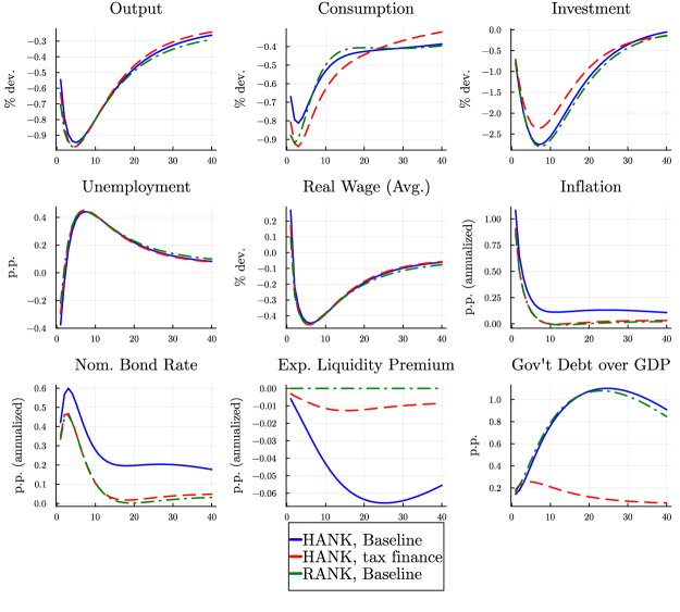
Figure 5: Model IRFs to 1% TFP shock

The blue solid lines in Figure 5 display Impulse Response Functions (IRFs) of the linearized baseline HANK economy in response to the TFP shock. Overall, they are mostly in line with the literature: Upon realization of the shock, output, consumption as well as investment drop since the economy’s potential is reduced. The investment reaction follows an $U$-shape due to the adjustment costs. However, the sluggish reaction of the central bank (which determines the nominal bond rate) does initially not crowd out demand as much as the fall in potential, which moderates the consumption drop on impact and actually induces a short-lived decrease in unemployment. Eventually though, the latter increases substantially, given that the AOB bargaining protocol induces only limited real wage responses. Inflation jumps up on impact as lower TFP increases marginal costs and initially falls relatively quickly once the central bank starts increasing the nominal rate. At the same time, public debt starts growing as the shock reduced tax revenues and requires more spending on unemployment benefits: due to the assumed slow pace of fiscal consolidation, the ratio of public debt to (annualized) GDP peaks at approximately 1 percentage point (p.p.) and remains above trend long after the shock. Furthermore, after a while, we observe inflation to plateau above its steady state level and hardly going down from there onwards, which induces the central bank to keep the nominal rate elevated as well. This is accompanied by a decrease in the liquidity premium, i.e. the real return on (liquid) bonds increase relative to the one on (illiquid) capital.
Overall, the results of the quantitative model are in line with the insights from the analytical model: The long-lived government debt expansion pushes up the neutral nominal rate on liquid assets, so that a central bank following a Taylor rule as in (37) will be confronted with similarly persistent inflation. While the quantitative magnitude appears to be of a moderate size, it effectively impedes going the “last mile” on disinflation after the shock. Recall also that the analyzed shock scenario induced a raise in the annual Public Debt-to-GDP ratio of only one percentage point. Of course, for a more substantial debt expansion we would expect the absolute effects to be larger.

5.2 Response under alternative fiscal policy

To further support the notion that the public debt dynamics after the shock are indeed the reason behind the persistently elevated inflation, I additionally consider a model counterfactual in which the fiscal authority holds both its debt and government consumption constant over time, i.e. $B_{t}=B_{ss}$ and $G_{t}=G_{ss}~{}\forall t$, and adjusts the tax rates to balance its budget without delay: The resulting dynamics are displayed as red-dashed lines in Figure 5. We see very similar dynamics for several real variables, such as output, unemployment and wages, although the model features a steeper consumption drop caused by the immediate tax increase upon impact of the shock. The change in the Debt-to-GDP ratio is only due to the impact of the TFP shock on its nominator. Now, in line with the intuition from the simple model, we see that under the alternative fiscal policy, inflation goes up less and is less persistent: it is approximately back at its steady state level after 10 quarters. In turn, the central bank also does not end up raising rates as much as in the baseline model. The faster decline of the real rate on liquid assets also stabilizes investment, which is not crowded out by additional government debt in this scenario.

5.3 Comparison with RANK/TANK

While the policy counterfactual above reaffirms the important role of public debt in shaping the inflation response to the supply shock, one may still have doubts whether the difference is actually driven by the mechanism outlined above. For example, the counterfactual fiscal policy also implies a substantially different time path for investment, which affects final goods demand and could in turn influence inflation.

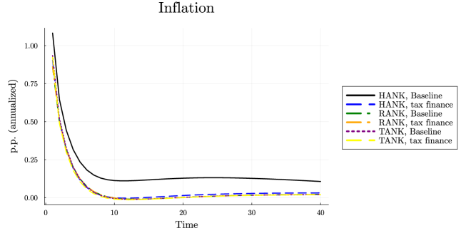
Figure 6: Inflation response in different model versions

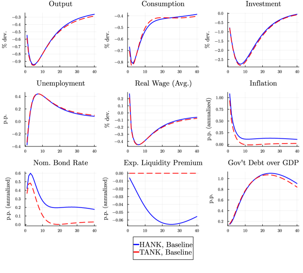
Figure 13: Model IRFs to 1% TFP shock

As an additional sanity check, it is therefore useful to consider the RANK and TANK versions of the model, which do not provide for effects of public debt on the natural rate of interest due them not featuring idiosyncratic income risk. The IRFs of the RANK model are additionally displayed as the green dot-dashed line in 5: Except the initial drop in consumption, they are broadly similar to the HANK model but feature inflation dynamics much closer to the HANK model under tax financing. Figure 13 in Appendix D additionally provides the IRFs of the TANK model and yields a similar picture, supporting the analytical result that the presence of income risk and not just high MPCs are the key driver of that “fiscal inflation”.
Finally, Figure 6 shows the inflation responses of all different model versions under the different fiscal policy scenarios, which we see to affect inflation dynamics only in the HANK economy.

5.4 The role of the asset market structure

As demonstrated in Section 4.3, the (long-run) elasticity of the model’s bond return with respect to government debt was crucially determined by how useful productive capital assets are for providing liquid assets suitable for self-insurance. In the model, this is determined by the cost parameter $\Psi$, which effectively stands in for various financial market frictions. Given that the model was intentionally calibrated so that this parameter does not affect its steady state, we are in a position to assess how the model’s aggregate response changes depending on the strength of said friction. To do so, I additionally compare the response of the baseline calibration to alternatives with $\Psi=0.0025$ and $\Psi=0.01$. As can be seen in Figure 3 in Section 4.3, the former induces a long-run response of the liquid bond rate of around 3 b.p., which corresponds to the lower end of the estimates from the literature. The latter is an ad hoc higher value.

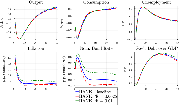
Figure 7: Model responses for different $\Psi$ values

Figure 7 presents model IRFs for these different cases: As we see, the precise value of $\Psi$ does only have a marginal impact on the real responses to the TFP shock but induces a noticeable higher (lower) medium-run inflation for an higher (lower) value of $\Psi$. This suggests the structure of the asset market to be a important factor for shaping inflation dynamics in HANK models.
 
Overall, the analysis in this section identified a noticeable effect of public debt on inflation dynamics in the aftermath of a negative supply shock. As the shock induced only a limited government debt expansion by itself, its overall quantitative magnitude was limited but very persistent. The latter is naturally a function of the exact fiscal policy rule in place and faster consolidation would make the “fiscal inflation” more short-lived.

6 Inflation after fiscal shocks

In addition to various supply side shocks, previous or concurrent government spending expansions have been argued to be additional drivers behind the 2022/2023 inflation bout (see e.g. de Soyres et al., 2022). As such policies can be inflationary also according to many theories not providing for effects of government debt on the natural rate of interest, it is relevant to evaluate the potential of that particular mechanism to influence inflation dynamics in the aftermath of such shocks. In this section, I do so in the context of a persistent shock to government consumption $G$, a standard scenario in the literature. However, similar insights apply to a “stimulus check” shock (see Appendix C.3).

6.1 Response to a Government spending shock

I begin by studying the response to a government spending shock that persistently increases $G$, which is assumed to increase by 0.5% of steady state GDP on impact and then revert back according to

$$\log(G_{t+1})=(1-\rho_{G})\log(G_{ss})+\rho_{G}\log(G_{t})$$

with $\rho_{G}=0.94$: This value implies an annual persistence of around $0.78$, similar to the value chosen by Auclert et al. (2023).

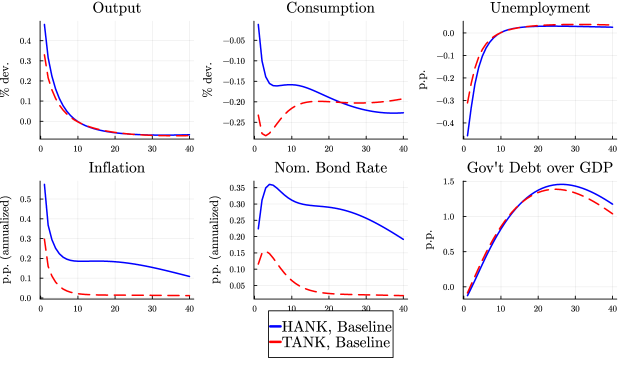
Figure 8: Model responses to the gov’t spending shock

Figure 8 displays the corresponding model responses, contrasting them with those of the TANK model version: Recall that the latter also deviates from Ricardian equivalence but does not allow for the additional feedback of public debt on the natural rate. Overall, in the HANK model the spending shock has approximately a unit multiplier on impact and substantially reduces unemployment. However, consumption declines after the shock, due to a) the central bank inducing a higher real interest rates due to the ensuing inflation and b) the eventually increasing tax rates necessary to consolidate the government budget. This is qualitatively consistent with the results of other HANK models (Kaplan and Violante, 2018). Overall, the government’s (annual) debt-to-GDP ratio increases by about 1.5% five years after the initial shock and is decreased slowly afterwards. At the same time, as for the TFP shock, inflation remains elevated long after the shock.
The results of the TANK model are qualitatively similar but several differences are apparent: The spending shock stimulates the economy less and consumption drops more on impact. Additionally, inflation does not only go up less but also lacks persistence. Of course, the different real dynamics align well with previous findings that households’ intertemporal MPCs matter substantially for the real effects of fiscal expansions and that these can be quite different between HANK and TANK models (Auclert et al., 2023). In contrast, the latter suggests that the inflationary pressure created by higher government debt may matter substantially for price dynamics after the fiscal shock, too.

6.2 Varying asset market structure

To further back up this conclusion, we can compare the aggregate model responses for different $\Psi$-values: Recall that this parameter determines the magnitude of the effect of public debt supply on liquid bond returns. So, if pressure on the neutral rate due to persistently higher public debt is an important driver of inflation after the fiscal shock, we should expect the response of the latter change substantially for different values of $\Psi$.

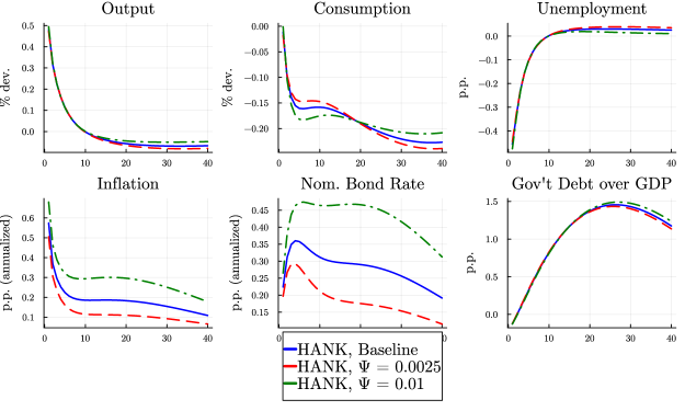
Figure 9: Model responses to spending shock for different $\Psi$

This is exactly what we see on Figure 9, with a lower (higher) $\Psi$ substantially decreasing (increasing) inflation after the shock. Of course, the result is also again testament to the importance of the asset market structure for inflation outcomes. But even for the low $\Psi=0.0025$, inflation remains noticeably elevated after the shock.
 
In conclusion, the inflationary effects of government debt present in HANK models are at least as relevant for the aggregate response to fiscal shocks as they are for supply shocks. Indeed, they appear even more pronounced for the latter. While this is partly mechanical due to the fiscal shock scenario resulting in a stronger debt expansion, the different unemployment response may also play a factor: in HANK models, the resulting higher idiosyncratic risk depresses interest rates and inflation (see e.g. Bayer et al., 2019), so that the effect should be stronger when a debt increase is accompanied by lower unemployment risk.

7 Implications for monetary policy

The previous two Sections established that according to HANK, increasing public debt in the aftermath of macroeconomic shocks generates additional inflationary pressure that lasts as long as debt is high. Naturally, central banks tasked with ensuring price stability would want to counteract such pressure. But how?
A natural possibility would be for the central bank to act more “hawkish”, i.e. react stronger to deviations of inflation from its target. This is also suggested by equation (15) that provided us intuition for the inflationary effects of public debt in Section 2.4: If the central bank operates a Taylor rule with a very high reaction to inflation $\theta_{\pi}$, $\tilde{\pi}_{1}$ will be affected less by changes in the “natural rate”. As “hawkish” policy for the model experiment below, I will consider the alternative value $\theta_{\pi}=2.0$ in interest rate rule (37).
However, we now know that the underlying issue is the increased government debt generating pressure on the neutral rate of interest. What if the monetary authority were to take this into account directly? Of course, the neutral rate is an unobservable object that can at best be estimated, but central banks obviously know the current state of public finances and could thus react to deviations of public debt from trend directly. In the model (and perhaps reality), this can be operationalized by adding a public debt term to interest rate rule (37):

$$\frac{R_{t+1}^{B}}{R^{B}_{SS}}=\left(\frac{R_{t}^{B}}{R^{B}_{SS}}\right)^{\rho^{R}}\left[\left(\frac{\pi_{t}}{\pi_{SS}}\right)^{\theta_{\pi}}\left(\frac{B_{t}}{B_{SS}}\right)^{\theta_{B}}\right]^{1-\rho^{R}}~{}~{}.$$ (41)

Below, I will refer to (41) as the “debt targeting” rule and use $\theta_{B}=0.004$, an ad hoc value that serves illustration purposes.

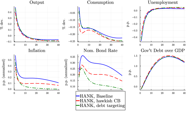
Figure 10: Model responses to gov’t spending shocks under different monetary rules

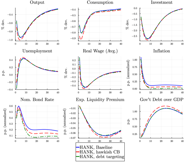
Figure 16: Model IRFs to TFP shocks for different policy rules

To assess the potential of the different interest rate rules to overcome the inflationary pressure from higher government debt, I contrast the resulting IRFs to the government spending shock in Figure 10. Clearly, either of the alternative rules is able to reduce the inflationary impact of the shock. However, we also see that a central bank that acts more “hawkish” but does not take into account public debt will still face inflation staying persistently above target, albeit at a lower level compared to the Baseline policy rule. Additionally, the “hawkish” policy comes at the cost of a stronger reduction in private consumption at impact and smaller responses of output and unemployment. This contrasts with the “debt targeting” rule, which yields slightly higher inflation at the time of the shock but achieves disinflation faster without any long-lasting “last mile” delays. Moreover, compared to the “hawkish” reaction, it gives rise to more favorable real dynamics, which are initially barely distinguishable from the Baseline response. Similar results arise for the case of the TFP shock, with an equivalent to Figure 10 being provided in Appendix D (Figure 16): The “debt targeting” rule achieves faster disinflation at lower real cost. So, according to HANK, fast disinflation after shocks accompanied by substantial increases in public debt requires monetary policy makers to sufficiently take into account the resulting upward pressure on liquid asset interest rates.

8 Robustness

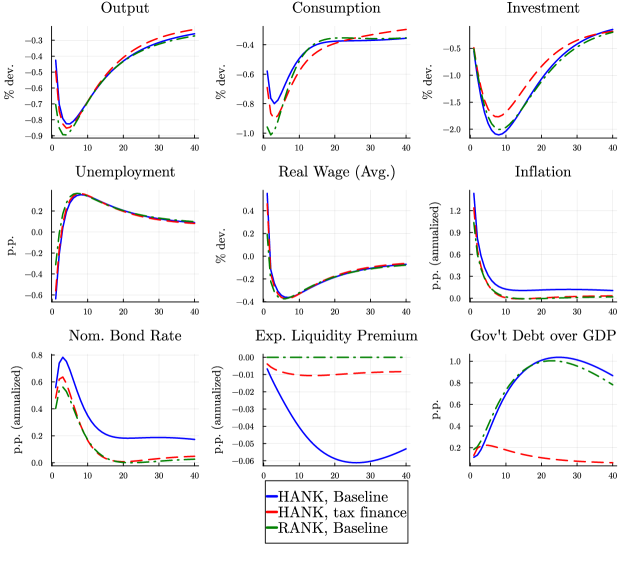
Figure 21: Model IRFs to TFP shocks under higher adjustment costs

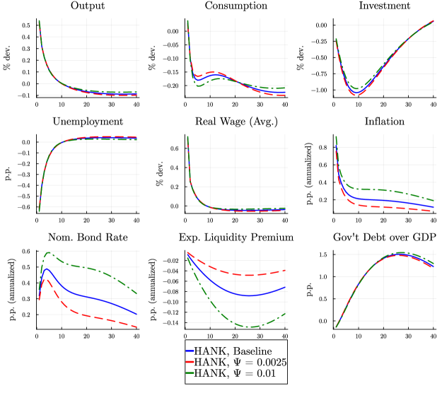
Figure 22: Model IRFs to gov’t spending shock shocks under higher adjustment costs

Given the complexity of the 2-asset HANK model used for the analysis above, one may naturally wonder whether the respective results hinge on a peculiar modelling assumption or calibration choice. To assuage related concerns, this section briefly discusses varies robustness checks I have conducted, with most details relegated to the Appendix.
Given the subject of the paper, one would hope that the results do not crucially depend on the particular choices of how fiscal policy is modeled. For example, the main text assumed that the fiscal authority consolidates it budget by raising the level of taxes $\tau$, even though we do not routinely observe government raising taxes in the aftermath of recessions. However, the discussion in Appendix C.1 reveals that similar results obtain if one assumes the government to never change tax rates but to adjust its spending $G$ instead.
Next, all government debt in the baseline model consisted of one-period bonds, which is clearly not the case in reality. While it is difficult to include a realistic maturity structure of public debt into a quantitative DSGE model, Appendix C.1 analyzes the implications of alternatively assuming a geometric maturity structure as used in the previous literature. While this induces somewhat larger valuation losses for bondholders at impact of an inflationary shock, it does not substantially affect model dynamics afterwards.
When thinking about the recent inflationary episode, one may also wonder to what extent the fiscal shock analyzed in Section 6 is a relevant scenario, given that many countries increased transfers instead of government consumption around that period. But as discussed in C.3, the insights from said exercise also apply to a “stimulus check” shock in which the fiscal authority pays out debt-financed surprise transfers to the model households.
Aside from fiscal policy itself, one may also worry about other aspects of the calibration: While many parameter choices are standard, this is not the case for the capital adjustment- and utilization cost parameters $\phi_{k}$ and $\delta_{2}/\delta_{1}$, the estimates for which vary considerably in the literature. I thus repeated the analysis for the alternative calibration $\varphi_{k}=7.5$ and $\delta_{2}/\delta_{1}=3.0$. However, as can be seen by inspecting Figure 21 in Appendix D, the different capital adjustment costs do not meaningfully impact inflation dynamics compared to the baseline model. This is also true for the fiscal policy shock results presented in Figure 22.
Another concern regarding the calibration may be that the baseline interest rate rule does not include a response to unemployment or the output gap. Would a “dual mandate” central bank also targeting either face a similar debt-driven inflation persistence? Figures 23 and 24 in Appendix D also display the aggregate responses if I set $\theta_{u}=0.15$ as in Gornemann et al. (2021). If anything, the unemployment response further increases inflation persistence after either shock.

9 Concluding Remarks

This work has theoretically studied the interaction between public debt and inflation, highlighting an additional channel for the former to affect the latter: If government debt obligations are useful beyond merely being a vehicle for intertemporal substitution, temporary increases in their supply affect equilibrium interest rates, which creates inflationary pressure if not explicitly taken into account by central banks.
For the purposes of this paper, the mentioned usefulness is micro-founded through households facing idiosyncratic risk and requiring liquid debt obligations for self-insurance due to the absence of a complete market for state-contingent assets. Other settings, in which different actors such as firms or banks value liquid government debt for self-insurance reasons, should have similar implications. Studying the quantitative magnitude of the channel in a state-of-the-art 2-asset HANK model required deviating from common assumptions on asset market structure in such models, which would have implied them to be either overly strong or weak. Eventually, I found the mechanism to be quantitatively relevant for both supply- and fiscal policy shocks: Although it implies its magnitude to be moderate compared to the overall inflation generated by these business cycle shocks, it can result in persistently elevated inflation in their aftermath so that going the “last mile” to disinflation takes a long time. However, according to the model, a central bank can avoid this outcome by explicitly reacting to deviations of public debt from its long-run trend. So, even if the sustainability of government budgets is taken as granted, monetary authorities should pay attention to government debt dynamics and calibrate their policy stance accordingly.
Ultimately, the conducted analyses also suggest topics for further work. In particular, it seems important to further study the implications of asset market arrangements for monetary and fiscal policy, which seem to be particularly pronounced if accounting for household heterogeneity and incomplete markets. I hope to do so in future work.

Appendix A Proofs for analytical model

A.1 Proof of Proposition 1

Let us first consider the First order condition for labor supply of an household of type $i\in\{h,l\}$:

$$\frac{w_{t}z^{i}}{c^{i}_{t}}=\gamma\frac{1}{1-N^{i}_{t}} \Leftrightarrow(1-N^{i}_{t})w_{t}z^{i}=\gamma\left(w_{t}z^{i}N^{i}_{t}+\frac{(1+i_{t})}{\pi_{t}}b_{it-1}-b_{it}-z^{i}\tau\right)$$ (42)

$$\Leftrightarrow N^{i}_{t}=\frac{1}{1+\gamma}\frac{1}{w_{t}z^{i}}\left(w_{t}z^{i}+\gamma(b_{it}+z^{i}\tau-\frac{(1+i_{t})}{\pi_{t}}b_{it-1})\right)$$ (43)

where the $c_{t}$ is substituted using the budget constraint in the second step. Summing up the labor supplied by both groups yields aggregate labor supply

$$N_{t} =\rho^{h}z^{h}N_{ht}+(1-\rho^{h})z^{l}N_{lt}$$

$$=\frac{1}{1+\gamma}\frac{\rho^{h}}{w_{t}}\left(w_{t}z^{h}+\gamma(b_{ht}+z^{h}\tau-\frac{(1+i_{t})}{\pi_{t}}b_{ht-1})\right)$$

$$~{}+\frac{1}{1+\gamma}\frac{1-\rho^{h}}{w_{t}}\left(w_{t}z^{l}+\gamma(b_{lt}+z^{l}\tau-\frac{(1+i_{t})}{\pi_{t}}b_{lt-1})\right)$$

$$=\frac{1}{1+\gamma}$$ (44)

The second step follows uses (1), bond market clearing condition

$$b^{g}_{t}=0=\rho^{h}b_{ht}+(1-\rho^{h})b_{lt}~{}~{}\forall t\geq 1$$

and in turn also $\tau_{t}=\frac{1+i_{t}}{\pi_{t}}b^{g}_{t-1}$ by the government budget constraint (7) and the assumed policy path.
Next, it is easy to see that either group of household’s intertemporal Euler equation will be of the form

$$c_{it+1}=\beta\frac{(1+i_{t+1})}{\pi_{t+1}}c_{it}~{}~{}.$$ (45)

Using again the budget constraints, we further obtain

$$\rho^{h}c_{ht}+(1-\rho^{h})c_{lt}=$$

$$\rho^{h}\left(w_{t}z_{h}N_{ht}+\frac{(1+i_{t})}{\pi_{t}}b_{ht-1}-b_{ht}-z_{h}\tau_{t}\right)$$

$$+(1-\rho^{h})\left(w_{t}z_{h}N_{ht}+\frac{(1+i_{t})}{\pi_{t}}b_{ht-1}-b_{ht}-z_{h}\tau_{t}\right)$$

$$=\frac{w_{t}}{1+\gamma}$$

after again using (1), (7), the bond market clearing condition and additionally (44). Naturally, absent profit incomes and capital investments, total household consumption must equal household labor income.
In turn, we can sum up (45) over types to obtain

$$\rho^{h}c_{ht+1}+(1-\rho^{h})c_{lt+1} =\beta\frac{(1+i_{t+1})}{\pi_{t+1}}(\rho^{h}c_{ht}+(1-\rho^{h})c_{lt})$$

$$\implies w_{t+1} =\beta\frac{(1+i_{t+1})}{\pi_{t+1}}w_{t}$$ (46)

Together with (6) and (5), (46) forms a system that characterizes the equilibrium of the model for $t\geq 1$. Since $r_{t}^{*}=\frac{1}{\beta}-1~{}~{}\forall t\geq 1$, it is easy to verify that $\pi_{t}=1$, $w_{t}=\frac{\epsilon-1}{\epsilon}$ and $i_{t}=r_{t}^{*}$ indeed solve that system. Local stability of this equilibrium is ensured by the Taylor principle.
Also, from the Euler equation it follows that in such an equilibrium, the consumption either household type $i\in\{h,l\}$ will be constant over time. Hence, we can back out their savings choice from the budget constraint for $t=1$ and $t=2$:

$$c^{i}_{1} =c^{i}_{2}$$

$$\Leftrightarrow w_{1}z^{i}N^{i}_{ss}+(1+i_{1})b_{i0}-b_{i1}-z^{i}\tau_{1} =w_{2}z^{i}N^{i}_{ss}+i_{ss}b_{i1}$$

$$\Leftrightarrow b_{i1} =\frac{1}{1+i_{ss}}\left((1+i_{1})b_{i0}-z^{i}\tau_{1}\right)$$

The second step uses that for $t\geq 1$, we need to have $b_{it+1}=b_{i+2}$ and since $c_{it}=c_{ss}$ as well as $w_{t}=w_{ss}\forall t\geq 1$, also $N^{i}_{t}=N^{i}_{ss}$ due to the first-order condition for labor supply. Using that result in (43), we obtain the labor supply as stated in the Proposition, which we can in turn use in the labor supply optimality condition as in (42) to back out the stated consumption schedule.

A.2 Proof of Proposition 2

Using that $1-N^{i}_{ss}=\gamma\frac{c^{i}_{ss}}{w_{ss}z^{i}}$ according to (9) and (10), we can derive the continuation value of a household that enters period $1$ with $b_{1}$ bonds and productivity draw $i\in\{h,l\}$ to be

$$V^{i}_{1}(b_{0})=\frac{1}{1-\beta}\left[(1+\gamma)\log\left(\frac{1}{1+\gamma}\left(w_{ss}z_{i}+\frac{i_{ss}}{1+i_{ss}}\left((1+i_{1})b_{0}-z^{i}\tau_{1}\right)\right)\right)+\gamma\log\frac{\gamma}{w_{ss}z_{i}}\right]$$

This allows us to state the problem of a household in period $0$ as

$$\max_{b_{0},N_{0}}\left\{\log(w_{0}N_{0}+T_{0}-b_{0})+\gamma\log(1-N_{0})+\beta\left[\rho^{h}V_{1}^{h}(b_{0})+(1-\rho^{h})V_{1}^{l}(b_{0})\right]\right\}$$

which has the following first order conditions:

$$N_{0}~{}:~{}~{}\frac{w_{0}}{w_{0}N_{0}+T_{0}-b_{0}} =\frac{\gamma}{1-N_{0}}$$

$$b_{0}~{}:~{}~{}\frac{1}{w_{0}N_{0}+T_{0}-b_{0}} =\beta\rho^{h}\frac{dV_{1}^{h}(b_{0})}{db_{0}}+\beta(1-\rho^{h})\frac{dV_{1}^{l}(b_{0})}{db_{0}}$$

$$=\frac{\beta}{1-\beta}\rho^{h}\frac{\frac{i_{ss}}{1+i_{ss}}(1+i_{1})}{\frac{1}{1+\gamma}\left(w_{ss}z^{h}+\frac{i_{ss}}{1+i_{ss}}\left((1+i_{1})b_{0}-z^{h}\tau_{1}\right)\right)}$$

$$+\frac{\beta}{1-\beta}\rho^{h}\frac{\frac{i_{ss}}{1+i_{ss}}(1+i_{1})}{\frac{1}{1+\gamma}\left(w_{ss}z^{l}+\frac{i_{ss}}{1+i_{ss}}\left((1+i_{1})b_{0}-z^{l}\tau_{1}\right)\right)}$$

Since households are identical in period $0$, they will make the same choices regarding bond-holdings. Thus, asset market clearing requires $b_{0}=b^{g}_{0}$ and in turn $b_{0}=T_{0}$ by the fiscal authority’s budget constraint. Using that in the first order condition for labor supply, we obtain $N_{0}=\frac{1}{1+\gamma}$. Since $c_{0}=w_{0}N_{0}+T_{0}-b_{0}$, it further follows that $c_{0}=\frac{w_{0}}{1+\gamma}$. Substituting these results into the first order condition for bond holdings, it simplifies to

$$\frac{1}{w_{0}} =\beta\rho^{h}\frac{(1+i_{1})}{\left(w_{ss}z^{h}+\frac{i_{ss}}{1+i_{ss}}\left((1+i_{1})b_{0}-z^{h}\tau_{1}\right)\right)}$$

$$+\beta(1-\rho^{h})\frac{(1+i_{1})}{\left(w_{ss}z^{l}+\frac{i_{ss}}{1+i_{ss}}\left((1+i_{1})b_{0}-z^{l}\tau_{1}\right)\right)}$$ (47)

which furthermore uses that $\frac{i_{ss}}{1+i_{ss}}=1-\beta$ due to the assumptions made above. Since we will have $\pi_{1}=1$ according to Proposition (1), it follows immediately from the Phillips curve (5) that

$$w_{0}=\frac{\phi(\pi_{0}-1)\pi_{0}+\epsilon-1}{\epsilon}~{}~{}.$$ (48)

Additionally, because of the assumed government policies, the tax rate in $t=1$ needs to fulfil

$$\rho^{h}z^{h}\tau_{1}+(1-\rho^{h})z^{l}\tau_{1}=\frac{1+i_{1}}{\pi_{1}}b^{g}_{0}\Leftrightarrow\tau_{1}=(1+i_{1})b^{g}_{0}$$

where the second step uses (1) and $\pi_{1}=1$. By substituting the above as well (48) and the Taylor rule (6) into (47), we obtain the equation that characterizes $\pi_{0}$ as stated in the Proposition:

$$\frac{\epsilon}{\epsilon-1+\phi(\pi_{t}-1)\pi_{t}} =\beta\rho^{h}\frac{1+r^{*}_{0}+\theta_{\pi}(\pi_{t}-1)}{w_{ss}z^{h}+\frac{i_{ss}}{1+i_{ss}}\left(1+r^{*}_{0}+\theta_{\pi}(\pi_{t}-1)\right)b^{g}_{0}(1-z_{h})}~{}~{}$$

$$+\beta(1-\rho^{h})\frac{1+r^{*}_{0}+\theta_{\pi}(\pi_{t}-1)}{w_{ss}z^{l}+\frac{i_{ss}}{1+i_{ss}}\left(1+r^{*}_{0}+\theta_{\pi}(\pi_{t}-1)\right)b^{g}_{0}(1-z^{l})}~{}~{}.$$

A.3 Proof of Proposition 3

By the Implicit Function Theorem, since $r_{0}^{n}(g^{0}_{b})$ is implicitly defined by $F(g^{b}_{0},r_{0}^{n}(g^{0}_{b}))=0$ with

$$F(g^{b}_{0},r_{0}^{n}) =\beta\rho^{h}\frac{1+r_{0}^{n}}{w_{ss}z^{h}+\frac{i_{ss}}{1+i_{ss}}\left(1+r^{n}_{0}\right)b^{g}_{0}(1-z^{h})}~{}~{}$$

$$+\beta(1-\rho^{h})\frac{1+r^{n}_{0}}{w_{ss}z^{l}+\frac{i_{ss}}{1+i_{ss}}\left(1+r^{n}_{0}\right)b^{g}_{0}(1-z^{l})}-\frac{\epsilon}{\epsilon-1}$$

we have

$$\frac{\partial r^{n}_{0}}{\partial b^{0}_{g}}=-\left.\frac{\partial F}{\partial b^{0}_{g}}\middle/\frac{\partial F}{\partial r^{n}_{0}}\right.~{}~{}.$$ (49)

The derivatives in (49) are given by

$$\frac{\partial F}{\partial b^{0}_{g}} =\beta\rho^{h}\frac{\frac{i_{ss}}{1+i_{ss}}(1+r_{0}^{n})^{2}(z^{h}-1)}{\left(w_{ss}z^{h}+\frac{i_{ss}}{1+i_{ss}}\left(1+r^{n}_{0}\right)b^{g}_{0}(1-z^{h})\right)^{2}}$$

$$+\beta(1-\rho^{h})\frac{\frac{i_{ss}}{1+i_{ss}}(1+r_{0}^{n})^{2}(z^{l}-1)}{\left(w_{ss}z^{h}+\frac{i_{ss}}{1+i_{ss}}\left(1+r^{n}_{0}\right)b^{g}_{0}(1-z^{l})\right)^{2}}$$ (50)

and

$$\frac{\partial F}{\partial r^{n}_{0}} =\beta\rho^{h}\frac{w_{ss}z^{h}}{\left(w_{ss}z^{h}+\frac{i_{ss}}{1+i_{ss}}\left(1+r^{n}_{0}\right)b^{g}_{0}(1-z^{h})\right)^{2}}$$

$$+\beta(1-\rho^{h})\frac{w_{ss}z^{l}}{\left(w_{ss}z^{l}+\frac{i_{ss}}{1+i_{ss}}\left(1+r^{n}_{0}\right)b^{g}_{0}(1-z^{l})\right)^{2}}~{}~{}.$$ (51)

Since $w_{ss}z^{h}>0$ and $w_{ss}z^{l}>0$, it is clear that $\frac{\partial F}{\partial r^{n}_{0}}>0$. However, things are less obvious for (50), as its first term is positive and its second term is negative since $z^{l}<1$. However, notice that if

$$\underbrace{w_{ss}z^{h}+\frac{i_{ss}}{1+i_{ss}}\left(1+r^{n}_{0}\right)b^{g}_{0}(1-z^{h})}_{=(1+\gamma)c^{h}_{ss}}>\underbrace{w_{ss}z^{l}+\frac{i_{ss}}{1+i_{ss}}\left(1+r^{n}_{0}\right)b^{g}_{0}(1-z^{l})}_{=(1+\gamma)c^{l}_{ss}}$$ (52)

then

$$\frac{\partial F}{\partial b^{0}_{g}} =\beta\rho^{h}\frac{\frac{i_{ss}}{1+i_{ss}}(1+r_{0}^{n})^{2}(z^{h}-1)}{\left((1+\gamma)c^{h}_{ss}\right)^{2}}+\beta(1-\rho^{h})\frac{\frac{i_{ss}}{1+i_{ss}}(1+r_{0}^{n})^{2}(z^{l}-1)}{\left((1+\gamma)c^{l}_{ss}\right)^{2}}$$

$$<\beta\rho^{h}\frac{\frac{i_{ss}}{1+i_{ss}}(1+r_{0}^{n})^{2}(z^{h}-1)}{\left((1+\gamma)c^{h}_{ss}\right)^{2}}+\beta(1-\rho^{h})\frac{\frac{i_{ss}}{1+i_{ss}}(1+r_{0}^{n})^{2}(z^{l}-1)}{\left((1+\gamma)c^{h}_{ss}\right)^{2}}=0~{}~{}$$

(the final equality follows from (1)). This means that if (52) holds, then $\frac{\partial F}{\partial b^{0}_{g}}<0$ and thus $\frac{\partial r^{n}_{0}}{\partial b^{0}_{g}}>0$. For that to be the case, we require

$$w_{ss}-\frac{i_{ss}}{1+i_{ss}}(1+r^{n}_{0}(b^{g}_{0}))b^{0}_{g}>0~{}~{}.$$ (53)

Under our restriction $0\leq b^{g}_{0}<\frac{\epsilon-1}{\epsilon}\frac{\beta}{1-\beta}=\frac{w_{ss}}{i_{ss}}$, this will be the case. Notice first that $r^{n}_{0}(b^{g}_{0})$ as implicitly defined by (13) fulfills

$$r^{n}_{0}(0)=\frac{1}{\beta\left(\frac{\rho^{h}}{z^{h}}+\frac{1-\rho^{h}}{z^{l}}\right)}-1<\frac{1}{\beta}-1=r^{n}_{0}\left(\frac{w_{ss}}{i_{ss}}\right)=i_{ss}$$ (54)

as $\frac{\rho^{h}}{z^{h}}+\frac{1-\rho^{h}}{z^{l}}>\frac{1}{\rho^{h}z^{h}+(1-\rho^{h})z^{l}}=1$ due to Jensen’s Inequality. Now, guess that (53) does hold for any $b^{g}_{0}\in[0,w_{ss}/i_{ss})$. In that case, our previous results imply that $r^{n}_{0}$ is increasing at any of these values. But then, as there is no discontinuity around $w_{ss}/i_{ss}$, (54) requires that we also must have $r^{n}_{0}(b^{g}_{0})<i_{ss}$ at these values. In turn, (53) is indeed true and we have $c^{h}_{ss}>c^{l}_{ss}$. So, it is also clear that $\frac{\partial r^{n}_{0}}{\partial b^{0}_{g}}<0$, establishing the proposition that $\frac{\partial r^{n}_{0}}{\partial b^{0}_{g}}>0$.

A.4 Proof of Proposition 4

We proceed similar as in Appendix (A.3). Given that (12) implicitly defines $\pi_{0}$ as a function of $b^{g}_{0}$ for given parameters,

$$\frac{\partial\pi_{0}}{\partial b^{0}_{g}}=-\left.\frac{\partial F^{\pi}}{\partial b^{0}_{g}}\middle/\frac{\partial F^{\pi}}{\partial\pi_{0}}\right.~{}~{}.$$ (55)

with

$$F^{\pi}(g^{b}_{0},\pi_{0}) =\beta\rho^{h}\frac{1+r^{*}_{0}+\theta_{\pi}(\pi_{0}-1)}{w_{ss}z^{h}+\frac{i_{ss}}{1+i_{ss}}\left(1+r^{*}_{0}+\theta_{\pi}(\pi_{0}-1)\right)b^{g}_{0}(1-z_{h})}~{}~{}$$

$$+\beta(1-\rho^{h})\frac{1+r^{*}_{0}+\theta_{\pi}(\pi_{0}-1)}{w_{ss}z^{l}+\frac{i_{ss}}{1+i_{ss}}\left(1+r^{*}_{0}+\theta_{\pi}(\pi_{0}-1)\right)b^{g}_{0}(1-z^{l})}-\frac{\epsilon}{\epsilon-1+\phi(\pi_{0}-1)\pi_{0}}$$

Similarly to (50), we have

$$\frac{\partial F^{\pi}}{\partial b^{0}_{g}} =\beta\rho^{h}\frac{\frac{i_{ss}}{1+i_{ss}}(1+r^{*}_{0}+\theta_{\pi}(\pi_{0}-1))^{2}(z^{h}-1)}{\left(w_{ss}z^{h}+\frac{i_{ss}}{1+i_{ss}}\left(1+r^{*}_{0}+\theta_{\pi}(\pi_{0}-1)\right)b^{g}_{0}(1-z^{h})\right)^{2}}$$

$$+\beta(1-\rho^{h})\frac{\frac{i_{ss}}{1+i_{ss}}(1+r^{*}_{0}+\theta_{\pi}(\pi_{0}-1))^{2}(z^{l}-1)}{\left(w_{ss}z^{h}+\frac{i_{ss}}{1+i_{ss}}\left(1+r^{*}_{0}+\theta_{\pi}(\pi_{0}-1)\right)b^{g}_{0}(1-z^{l})\right)^{2}}~{}~{}.$$ (56)

Additionally,

$$\frac{\partial F^{\pi}}{\partial\pi_{0}}=\beta\rho^{h}\frac{\theta_{\pi}w_{s}sz^{h}}{(1+\gamma)c^{h}_{ss}}+\beta(1-\rho^{h})\frac{\theta_{\pi}w_{s}sz^{l}}{(1+\gamma)c^{l}_{ss}}+\frac{\epsilon\phi(2\pi_{0}-1)}{(\epsilon-1+\phi(\pi_{0}-1)\pi_{0})^{2}}~{}~{}.$$

Since we are considering the derivative around $r^{*}=r^{n}_{0}(b^{0}_{g})$ at which $\pi_{0}=1$, $2\pi_{0}-1>0$ so all the terms are positive and $\frac{\partial F^{\pi}}{\partial\pi_{0}}>0$.
Regarding (56), we can use the same argument as in Appendix (A.3). If $c^{h}_{ss}>c^{l}_{ss}$, then

$$\frac{\partial F^{\pi}}{\partial b^{0}_{g}} =\beta\rho^{h}\frac{\frac{i_{ss}}{1+i_{ss}}(1+r^{*}_{0}+\theta_{\pi}(\pi_{0}-1))^{2}(z^{h}-1)}{\left((1+\gamma c^{h}_{ss})\right)^{2}}+\beta(1-\rho^{h})\frac{\frac{i_{ss}}{1+i_{ss}}(1+r^{*}_{0}+\theta_{\pi}(\pi_{0}-1))^{2}(z^{l}-1)}{\left((1+\gamma c^{l}_{ss})\right)^{2}}$$

$$<\beta\rho^{h}\frac{\frac{i_{ss}}{1+i_{ss}}(1+r^{*}_{0}+\theta_{\pi}(\pi_{0}-1))^{2}(z^{h}-1)}{\left((1+\gamma c^{h}_{ss})\right)^{2}}+\beta(1-\rho^{h})\frac{\frac{i_{ss}}{1+i_{ss}}(1+r^{*}_{0}+\theta_{\pi}(\pi_{0}-1))^{2}(z^{l}-1)}{\left((1+\gamma c^{h}_{ss})\right)^{2}}=0$$

Again, we are considering the case with $r^{*}_{0}=r^{n}_{0}(b^{0}_{g})$ for some $b^{0}_{g}\in[0,w_{ss}/i_{ss})$, so from the analysis in Appendix A.3, we know that indeed $c^{h}_{ss}>c^{l}_{ss}$ in this case. Thus $\frac{\partial F^{\pi}}{\partial b^{0}_{g}}<0$ and hence $\frac{\partial\pi_{0}}{\partial b^{0}_{g}}>0$, which establishes the proposition.

Appendix B Details on quantitative HANK model

B.1 Wage determination

During the $M$ subperiods of a period’s production stage (compare Section 3.1), the worker and the labor agency take turns extending wage offers: I will be denoting variables on a per-subperiod basis with a $\Delta$, e.g. $h_{\Delta,t}:=\frac{h_{t}}{M}$ is the revenue a labor agency for producing during one of the sub-periods etc..
I assume that in any given period, the labor agency gets to make the first offer. If the worker rejects it, she can make a counter-offer in the next period that the firm can reject or accept, and so on. Once a wage agreement has been reached, the match starts producing labor services and the worker is paid the agreed wage rate for the remainder of the period. However, before that happens, an agency matched with a skill $s$-worker incurs a cost of delay $\gamma_{\Delta}(s)$ per sub-period, while the worker will receive an outside income $\tilde{b}_{\Delta,t}(s)$ per sub-period. Both these values will have to depend on the respective’s workers productivity $s$ to avoid high (low) productivity workers being able to bargain wages that are disproportionately low (high) comparatively to their skill. If no wage is accepted before the last period $M$, the worker gets to make a take-it-or-leave-it offer during the last sub-period ($M$ is even). If rejected by the firm, the match irreparably dissolves and the worker enters the pool of the unemployed.
Now, to characterize the wage outcome, we first note that independently of worker wealth, a worker (agency) in our model would always like the wage to be as high (low) as possible. In turn, it is optimal for each party to make offers barely acceptable to the other. Hence, slightly abusing notation, if a firm gets to make an wage offer $w^{f}_{j,\Delta,t}$ to a worker in a sub-period $j<M$, this offer should fulfill

$$V\left((1-\tau^{y})[(M-j+1)w^{f}_{j,\Delta,t}+(j-1)\tilde{b}_{\Delta,t}(s)],\cdots\right)$$

$$= V\left((1-\tau^{y})[(M-j)(1-\tau^{w})w^{w}_{j+1,\Delta,t}(s)+j\tilde{b}_{\Delta,t}(s),\cdots]\right)$$ (57)

with $V$ being a value functions as in (21) or (22), having added $y_{t}$ as additional input. The left-hand side is the value a worker would obtain from accepting the offer, while the right-hand side is the value of not accepting and making the equilibrium counter-offer $w^{w}_{j+1,\Delta,t}(s)$ in the next sub-period (which will be accepted). Since $V$ as in (21), (22) is strictly increasing in income (additional resources can always be consumed), (57) implies

$$(M-j+1)w^{f}_{j,\Delta,t}(s)+(j-1)\tilde{b}_{\Delta,t}(s)=(M-j)w^{w}_{j+1,\Delta,t}(s)+j\tilde{b}_{\Delta,t}(s)~{}~{}.$$ (58)

Intuitively, worker wealth does not matter for in indifference condition (57), as any worker prefers higher period income in our setting. Similarly, if a worker gets to make an wage offer $w^{f}_{j,\Delta,t}$ to a firm in a subperiod $j<M$, this offer should fulfill

$$(M-j+1)(h_{\Delta,t}s-w^{w}_{j,\Delta,t}(s))=-\gamma_{\Delta}(s)+(M-j)(h_{\Delta,t}s-w^{f}_{j+1,\Delta,t}(s))~{}~{}.$$ (59)

Finally, if no wage is accepted until period $j=M$, the indifference condition for an agency contemplating a worker’s offer $w^{w}_{M,\Delta,t}$ would be

$$h_{\Delta,t}s-w^{w}_{M,\Delta,t}(s)+(1-\zeta)(1-\delta(s_{t}))\beta\mathbb{E}_{t}J(s_{t+1},\Gamma_{t})=0$$ (60)

as, if rejecting the offer, the firm would have to look for a new worker, the value of which is $0$ due to free entry. We note that worker wealth does not enter indifference condition (60) either, as any worker would like to claim the maximum possible amount of income during the final bargaining period.
Since the equilibrium wage outcome can be characterized using equations (58), (59) and (60), it follows that our AOB bargaining scheme delivers wages that are independent of worker wealth:

Proposition 5.

The per-period wage of a matched worker with labor productivity $s$ will be given by

$$w_{t}(s)=\frac{1}{2}\left(h_{t}s+\tilde{b}_{t}(s)\right)+\frac{M-2}{2M}\gamma(s)+(1-\zeta)(1-\delta(s_{t}))\beta\mathbb{E}_{t}J(s_{t+1},\Gamma_{t})~{}~{}.$$ (61)

Proof.

Re-arranging indifference conditions (58) and (59) yields

$$w^{f}_{j,\Delta,t}(s)=\frac{\tilde{b}_{\Delta,t}(s)}{(M-j+1)}+\frac{M-j}{M-j+1}w^{w}_{j+1,\Delta,t}(s)$$ (62)

and

$$w^{w}_{j,\Delta,t}(s)=\frac{\gamma_{\Delta}(s)+h_{\Delta,t}s}{M-J+1}+\frac{M-j}{M-j+1}w^{f}_{j+1,\Delta,t}(s)$$ (63)

which we can combine to obtain

$$w^{w}_{j,\Delta,t}(s)=\frac{\gamma_{\Delta}(s)+h_{\Delta,t}s+\tilde{b}_{\Delta,t}(s)}{M-j+1}+\frac{M-j-1}{M-j+1}w^{w}_{j+2,\Delta,t}(s)~{}~{}.$$ (64)

Iterating (64) forward $M/2-1$ times, we obtain

$$w^{w}_{2,\Delta,t}(s)=\frac{M-2}{2}\frac{\gamma_{\Delta}(s)+h_{\Delta,t}s+\tilde{b}_{\Delta,t}(s)}{M-1}+\frac{1}{M-1}w^{w}_{M,\Delta,t}(s)$$

which we can use in (62) for $j=1$ to get

$$w^{f}_{1,\Delta,t}(s)=\tilde{b}_{\Delta,t}(s)+\frac{M-2}{2}\frac{\gamma_{\Delta}(s)+h_{\Delta,t}s+\tilde{b}_{\Delta,t}(s)}{M}+\frac{1}{M}w^{w}_{M,\Delta,t}(s)~{}~{}.$$ (65)

Substituting (60) and re-arranging, we obtain the equilibrium subperiod 1 offer extended by the firm

$$w^{f}_{1,\Delta,t}(s)=\frac{1}{2}\left(h_{\Delta,t}s+\tilde{b}_{\Delta,t}(s)\right)+\frac{M-2}{2M}\gamma_{\Delta}(s)+\frac{1}{M}(1-\zeta)(1-\delta(s_{t}))\beta\mathbb{E}_{t}J(s_{t+1},\Gamma_{t})$$ (66)

which will be accepted. In turn, the period wage is this wage times $M$, i.e.

$$w_{t}(s)=\frac{1}{2}\left(h_{t}s+\tilde{b}_{t}(s)\right)+\frac{M-2}{2M}\gamma(s)+(1-\zeta)(1-\delta(s_{t}))\beta\mathbb{E}_{t}J(s_{t+1},\Gamma_{t})~{}~{}.$$

∎

B.2 Definition of equilibrium

Definition 1.

A Recursive Equilibrium of the model consists of

• value functions $V^{a}(a_{it},k_{it},e_{it},s_{it},\Psi_{it};\Gamma_{t})$, $V^{na}(a_{it},k_{it},e_{it},s_{it},\Psi_{it};\Gamma_{t})$ and $J(s_{it},\Gamma_{t})$,

• household policies $a^{a}(a_{it},k_{it},e_{it},s_{it},\Psi_{it};\Gamma_{t})$, $a^{na}(a_{it},k_{it},e_{it},s_{it},\Psi_{it};\Gamma_{t})$, $k(a_{it},k_{it},e_{it},s_{it},\Psi_{it};\Gamma_{t})$ and $c^{a}(a_{it},k_{it},e_{it},s_{it},\Psi_{it};\Gamma_{t})$, $c^{na}(a_{it},k_{it},e_{it},s_{it},\Psi_{it};\Gamma_{t})$,

• firm sector policies $I_{t}$, $K_{t}$, $H_{t}$, $Y_{t}$, $u_{t}$, $\theta_{t}$,$B_{t}^{l}$, $\Pi_{t}$,$y_{jt}\forall j\in[0,1]$

• prices $h_{t}$, $r_{t}$, $q_{t}$, $r_{t}^{l}$, $mc_{t}$

• a wage schedule $w_{t}(s)\forall s\in\mathcal{S}$,

• government policies $b_{t}(s),G_{t},B_{t+1},\tau_{t}^{y},R_{t+1}^{B}$,

• measures $m_{t}(\cdot)$,

so that

1. Given prices $r_{t}^{l}$, $r_{t}$, $q_{t}$, wage schedule $w_{t}(s)$ and profits $\Pi_{t}$ as well as labor market tightness $\theta_{t}$, the value functions $V^{a}(a_{it},k_{it},e_{it},s_{it},\Xi_{it};\Gamma_{t})$, $V^{na}(a_{it},k_{it},e_{it},s_{it},\Xi_{it};\Gamma_{t})$ solve the households’ Bellman equations in (21) and (22) and $a(a_{it},k_{it},e_{it},s_{it},\Xi_{it};\Gamma_{t})$, $k(a_{it},k_{it},e_{it},s_{it},\Xi_{it};\Gamma_{t})$, $c(a_{it},k_{it},e_{it},s_{it},\Xi_{it};\Gamma_{t})$ are the resulting optimal policy functions.

2. $y_{jt}\in[0,1]$ are consistent with demand schedule (4) and final output $Y_{t}$ given by (3).

3. Inflation $\pi_{t}$ is consistent with Phillips curve (23).

4. Given prices $h_{t}$, $r_{t}$, $q_{t}$, $mc_{t}$ and technology shock $Z_{t}$ the intermediate goods producers choices $K_{t},H_{t},u_{t}$ are consistent with optimality conditions (25)-(27).

5. Given price $q_{t}$, the intermediate goods producers choices $I_{t}$ are consistent with optimality condition (28).

6. Given prices $h_{t}$ and wage schedule $w_{t}(s)$, labor agency value functions $J(s_{it},\Gamma_{t})$ are consistent with (29).

7. The wage schedule $w_{t}(s)$ is consistent with bargaining outcome (33).

8. Labor market tightness $\theta_{t}$ is consistent with free-entry condition (32).

9. The Liquid Asset Funds’ portfolio choice is consistent with (35).

10. The return of liquid assets is given by (71).

11. Given inflation $\pi_{t}$ and unemployment $u_{t}$, the monetary authority set $R_{t+1}^{B}$ according to (37).

12. Taking the remaining values as given, the government sets taxes according to (LABEL:eq:tax_rule) and issues debt $B_{t+1}$ so that (38) holds.

13. The market for liquid asset clears, i.e.

    $$A^{l}_{t}=\int^{\infty}_{\underline{a}}a_{it}m_{t}(a_{it})da_{it}~{}~{}.$$

14. The government bond market clears, i.e.

    $$B^{l}_{t}=B^{g}_{t}~{}~{}.$$

15. Capital market clearing requires, i.e.

    $$K_{t}=\frac{A^{l}_{t}-B^{l}_{t}}{q_{t-1}}+\int^{\infty}_{0}k_{it}m_{t}(k_{it})dk_{it}~{}~{}.$$

16. The market for investment good clears, i.e.

    $$K_{t+1}=(1-\delta(u_{t}))K_{t}+\left[1-\frac{\phi}{2}\left(\frac{I_{t}}{I_{t-1}}-1\right)^{2}\right]I_{t}$$

17. The market for labor services clears, i.e.

    $$H_{t}=\sum_{s\in\mathcal{S}}sm_{t}^{e}(s)~{}~{}.$$

18. The market for intermediate goods clears, i.e.

    $$\int^{1}_{0}y_{t}(j)dj=F_{t}(u_{t}K_{t},H_{t})$$

19. The final good market clears, i.e.

    $$Y_{t}= C_{t}+G_{t}+I_{t}+\frac{\phi}{2}\left[\frac{I_{t}}{I_{t-1}}-1\right]^{2}+\kappa V_{t}+\bar{R}\int^{0}_{\underline{a}}a_{it}m_{t}(a_{it})da_{it}$$

    $$-\left[\phi+\frac{\Psi}{2}\left(1-\frac{B_{t}^{l}}{A_{t}^{l}}\right)^{2}\right]A_{t}^{l}~{}~{}.$$

20. The dynamics of measures $m_{t}(\cdot)$ is consistent as described in Appendix B.3

B.3 Details on measures $m$

Formally, $m_{t}$ describes a probability measure on the measurable space $(\mathcal{X},\mathcal{A})$, with $\mathcal{X}:=[\underline{a},\infty]\times\mathbb{R}_{+}\times[0,1]\times\mathcal{S}\times[0,1]$ and $\mathcal{A}:=\mathbf{B}([\underline{a},\infty])\times\mathbf{B}(\mathbb{R}_{+})\times\mathbf{P}([0,1])\times\mathbf{P}(\mathcal{S})\times\mathbf{P}([0,1])$, where $\mathbf{P}(\cdot)$ denotes the power set and $\mathbf{B}(\cdot)$ the Borel $\sigma$-algebra of a given set.
Practically, with some abuse of notation, we have $m_{t}(\cdot)$ describe the masses of households in a particular state at the beginning at period $t$, i.e $m_{t}(a=a_{i},k=k_{i},e=e_{i},s=s_{i},\Xi=\Xi_{i})$ is the mass of households with assets $a_{i},k_{i}$, employment status $e_{i}$, skill $s_{i}$ and “entrepreneur status” $\Xi_{i}$. For ease of notation above, I suppress states that are fully integrated over, e.g.

$$m_{t}(a=a_{i},e=e_{i})=\sum_{\Xi_{i}\in\{0,1\}}\sum_{s_{i}\in\mathcal{S}}\int^{\infty}_{0}m_{t}(a=a_{i},k=k_{i},e=e_{i},s=s_{i},\Xi=\Xi_{i})dk_{i}$$ (67)

denotes the mass of households with employment status $e_{i}$ and bond holdings $a_{i}$. Additionally, I suppress the annotation of non-suppressed inputs whenever it does not cause any confusion, i.e. we may write $m_{t}(e_{i})=m_{t}(e=e_{i})$.
Naturally, to be consistent with a unit mass of households, we require

$$\sum_{e_{i}\in\{0,1\}}\sum_{\Xi_{i}\in\{0,1\}}\sum_{s_{i}\in\mathcal{S}}\int^{\infty}_{0}\int^{\infty}_{\underline{a}}m_{t}(a=a_{i},k=k_{i},e=e_{i},s=s_{i},\Xi=\Xi_{i})da_{i}dk_{i}=1~{}~{}.$$

Additionally, the evolution of measures also need to be consistent with household choices. Defining

$$\tilde{X}^{na}(a^{\prime},k,e,s,\Psi;\Gamma_{t}) :=\left\{a\in[\underline{a},\infty):~{}a^{na}(a,k_{it},e_{it},s_{it},\Psi_{it};\Gamma_{t})=a^{\prime}\right\}$$

$$\tilde{X}^{a}(\{a^{\prime},k^{\prime}\},e,s,\Psi;\Gamma_{t}) :=\left\{\{a,k\}\in[\underline{a},\infty)\times\mathbb{R}_{+}:~{}a^{a}(a,k,s,\Psi;\Gamma_{t})=a^{\prime}~{}~{}\text{and}~{}~{}\right.$$

$$\left.~{}~{}k(a,k,e,s,\Psi;\Gamma_{t})=k^{\prime}\right\}$$

as well as the “middle of period” measure $\tilde{m}_{t}(a,k,e,s,\Xi)$ fulfilling

$$\tilde{m}_{t}(a,k,e=1,s,\Xi=0) =p_{t}^{UE}m_{t}(a,k,e=0,s,\Xi=0)+(1-\delta(s)+\delta(s)p_{t}^{UE})m_{t}(a,k,e=1,s,\Xi=0)$$

$$\tilde{m}_{t}(a,k,e=0,s,\Xi=0) =(1-p_{t}^{UE})m_{t}(a,k,e=0,s,\Xi=0)+\delta(s)(1-p_{t}^{UE})m_{t}(a,k,e=1,s,\Xi=0)$$

$$\tilde{m}_{t}(a,k,e,s,\Xi=1) =m_{t}(a,k,e,s,\Xi=1)$$

means they must follow

$$m_{t+1}(a,k,e,s,\psi=0)=$$

$$(1-\zeta)\sum_{s_{t}\in\mathcal{S}}\Pi^{s}(s,|s_{t},e)\left(\lambda\int_{\tilde{X}^{a}(\{a,k\},e,s_{t},\Xi=0;\Gamma_{t})}d\tilde{m}_{t}(a_{it},k_{it},s_{t},\Xi_{t}=0)\right.$$

$$+\left.(1-\lambda)\int_{\tilde{X}^{na}(a,k,e,s_{t},\Xi=0;\Gamma_{t})}d\tilde{m}_{t}(a_{it},k,s_{t},\Xi_{t}=0)\right)$$

$$+\iota p_{s}\left(\lambda\int_{\tilde{X}^{a}(\{a,k\},e,s,\Xi=1;\Gamma_{t})}d\tilde{m}_{t}(a_{it},k_{it},\Xi_{t}=1)+(1-\lambda)\int_{\tilde{X}^{na}(a,k,e,s,\Xi=1;\Gamma_{t})}d\tilde{m}_{t}(a_{it},k,\Xi_{t}=1)\right)$$

and

$$m_{t+1}(a,k,e=0,\psi=1)=$$

$$\zeta\left(\lambda\int_{\tilde{X}^{a}(\{a,k\},e,s,\Xi=0;\Gamma_{t})}d\tilde{m}_{t}(a_{it},k_{it},\Xi_{t}=0)+(1-\lambda)\int_{\tilde{X}^{na}(a,k,e,s,\Xi=0;\Gamma_{t})}d\tilde{m}_{t}(a_{it},k,\Xi_{t}=0)\right)$$

$$+ (1-\iota)\left(\lambda\int_{\tilde{X}^{a}(\{a,k\},e,s,\Xi=1;\Gamma_{t})}d\tilde{m}_{t}(a_{it},k_{it},\Xi_{t}=1)+(1-\lambda)\int_{\tilde{X}^{na}(a,k,e,s,\Xi=1;\Gamma_{t})}d\tilde{m}_{t}(a_{it},k,\Xi_{t}=1)\right)$$

Finally measures $m_{t}^{e},m_{t}^{u}$ and $m_{t}^{\Psi}$ will fulfill

$$m_{t}^{e}=\sum_{s\in\mathcal{S}}\left[(1-\delta(s)+\delta(s)p_{t}^{UE})m_{t}(e=1,s)+p_{t}^{UE}m_{t}(e=0,s)\right]$$

as well as

$$m_{t}^{u}=\sum_{s\in\mathcal{S}}\left[\delta(s)(1-p_{t}^{UE})m_{t}(e=1,s)+(1-p_{t}^{UE})m_{t}(e=0,s)\right]~{}~{}.$$

B.4 Details on numerical implementation

B.4.1 Details on Steady State Solution

The household problem needs to be solved on a discretization of the state space: I choose $70$ grid points for both $a$ and $k$, either of which are non-linearily spaced as household decision functions tend to be more non-linear for lower levels of assets. In particular, the grid points for both $a$ for $k$ are spaced according to the “double exponential” rule, i.e.

$$\mathcal{X}=x_{min}+\exp(\exp(\mathbf{u}(\log(1+\log(1+x_{max}-x_{min})),n_{i}))-1)-1$$

where $x_{min}$ is the minimum value on the grid for variable $x$, $x_{max}$ the maximum value and $\mathbf{u}(0,x_{max})$ a vector of equidistant points on the interval $[0,x_{max}]$. Since household value- and policy functions will feature and additional kink around $a=0$ when the borrowing penalty kicks in, I add 5 additional grid points in the immediate vicinity of that point. Given that individual labor productivity is discretized to $13$ points, this means that the household problem is solved on a tensor grid of $70\times 70\times(2\times 13+1)=132300$ points (the “entrepreneur” status adds an additional “income” state to the $2\times 13$ for employed and unemployed workers). The discretization of the individual labor productivity process is described in the main text, Section 4. Whenever interpolation is needed off the grid, I use linear interpolation
For the implementation of the multidimensional EGM algorithm, I follow the replication codes for Bayer et al. (forthcoming) closely. Given the random illiquid asset adjustment, the EGM scheme only iterates over marginal value functions (i.e. the derivatives of $V$ with respect to $m$ and $k$) and does not compute $V$ directly.For finding the steady, I iterate over $r^{l}_{ss}$ and $r^{k}_{ss}$: Given these values, the remaining steady variables can be backed out and the household-problem solved. I then use a heuristic updating procedure to search for $r^{l}_{ss}$ and $r^{k}_{ss}$ so that the asset markets clear.

B.4.2 Details on Perturbation

As already indicated in the main text, the model’s dynamic equilibrium is approximated using First-Order Perturbation around the its non-stochastic steady state.
For the perturbation, note that when using the discretized representations of the marginal value functions as well as the joint income/asset distribution, the equilibrium can be represented as the solution to a non-linear difference equation of the form

$$\mathbb{E}_{t}F(\mathbf{y_{t}},\mathbf{x_{t}},\mathbf{y_{t+1}},\mathbf{x_{t+1}})=0$$ (68)

as e.g. used by Schmitt-Grohe and Uribe (2004). $\mathbf{y}$ denotes a vector of control variables, which includes the households’ marginal value functions on the grid and $\mathbf{x}$ a vector of state variables, which includes the discretized distribution.
In theory, one could find the linearized equilibrium using the standard approach of computing the Jacobians of $F$ as in (68) and then solve the resulting linear difference equation relying on methods such as Klein (2000). In practice, however, such an approach would involve very high computational costs for the 2-asset HANK model, given that the full $\mathbf{y}$ and $\mathbf{x}$ have a combined length exceeding $300,000$.
To overcome this problem, I use the approach by Bayer and Luetticke (2020), which conducts dimension reduction steps before computing the Jacobians. Specifically, it first uses a Discrete Cosine Transform (DCT) to dimension-reduce the marginal value functions: The values resulting from such a DCT are coefficients of the fitted multidimensional Chebychev polynomial, and, importantly, their absolute values have an interpretation as measuring the “importance” of the corresponding polynomial for fitting the data. In turn, instead of perturbing the discretized marginal value functions directly, one perturbs only the largest of these DCT coefficients, with the others fixed at their steady state values. For this application, I perturb the DCT coefficients accounting for 99.995% of their total Euclidean norm.
For reducing the dimensionality of the joint distribution, Bayer and Luetticke (2020) furthermore suggest to split it into marginals and a copula, where the latter is in effect treated as a interpolator mapping the steady state marginal distributions into the joint distribution. That “interpolator” can also be dimension-reduced through a DCT or just kept fixed, so one only perturbs the marginals as well as selected coefficients of the copula, which have substantially lower dimension.
In the presented set-up featuring the binary employment status, a potential problem is that there is no unique way to define a marginal CDF over the income states for the split (or, equivalently, that the copula is not unique). To sidestep this issue, I dimension-reduce the joint distribution of employed and unemployed agents separately, which somewhat limits the amount of dimension reduction that can be achieved. However, even despite that, the procedure manages to shrink the effective dimensionality of the system to a manageable number of approx. 1,800.

B.5 Additional model parameters

The model parameters not explicitly stated in Section 4 are provided in Table 5.

	$s$	$\gamma(s)$	$\delta(s)$
$s_{1}$	0.1384	0.1282	0.1266
$s_{2}$	0.1729	0.1601	0.123
$s_{3}$	0.2157	0.1997	0.1184
$s_{4}$	0.2689	0.249	0.113
$s_{5}$	0.3353	0.3105	0.1065
$s_{6}$	0.4188	0.3871	0.099
$s_{7}$	0.5212	0.4826	0.0903
$s_{8}$	0.6498	0.6016	0.0806
$s_{9}$	0.81	0.74	0.07
$s_{1}0$	1.0096	0.9348	0.0586
$s_{11}$	1.2585	1.1652	0.0470
$s_{12}$	1.5685	1.4523	0.0357
$s_{13}$	1.96	1.815	0.02533

Table 5: Skill-specific parameters

Appendix C Robustness

C.1 Alternative fiscal rule

As an alternative to the baseline fiscal rule (40), I consider the case of the government always keeping taxes constant at its steady state level $\tau_{t}=\tau_{ss}$ and instead gradually reduces its spending $G$ over time to reduce its budget. In particular, I assume $G$ to follow the rule

$$\frac{G_{t}}{G_{ss}}=\left(\frac{G_{t-1}}{G_{ss}}\right)^{\rho_{G}}\left(\frac{B_{t}}{B_{ss}}\right)^{(1-\rho_{G})\psi_{B}}$$ (69)

also used by Bayer et al. (2023b) and use $\rho_{G}=0.94$ and $\psi_{B}=-0.75$.
To briefly convey the impact of this alternative assumption, Figures 17 and 18 display model responses for the TFP- and government spending shock under this alternative assumptions.
Under rule (69) and the chosen parameterization, the government debt increase is somewhat less pronounced and persistent after the shocks. At the same time, we see milder but still noticeable inflation persistence after the shocks, affirming the robustness to the alternative assumption on fiscal policy but providing a case in point for the importance of government debt dynamics for inflation in the aftermath of macroeconomic shocks.

C.2 Long-term government debt

For introducing long-term governments bonds, I follow Bayer et al. (2023a), who consider a setting featuring a simple geometric maturity structure. Bonds are long-lived. Every period, they pay one nominal unit of return and a fraction $\delta^{B}$ of them retire without repaying the principal. Denoting the nominal period $t$ price of a bond as $Q_{t}^{B}$, their expected nominal return is thus given by

$$\mathbb{E}_{t}\frac{Q_{t+1}^{B}(1-\delta^{B})+1}{Q_{t}^{B}}~{}~{}.$$

As before, similar to the baseline model, the government bonds are not directly held by the households but instead by the LAFs whose problem becomes

$$\max_{B^{l}_{t+1}}\left\{\mathbb{E}_{t}\left[(r_{t+1}^{k}+q_{t+1})\frac{A_{t+1}^{l}-B_{t}^{l}}{q_{t}}+\frac{Q_{t+1}^{B}(1-\delta^{B})+1}{\pi_{t+1}Q_{t}^{B}}B^{l}_{t+1}\right]-A_{t+1}^{l}\left(\varphi+\frac{\Psi}{2}\left(1-\frac{B_{t+1}^{l}}{A_{t+1}^{l}}\right)^{2}\right)\right\}~{}~{}~{},$$ (70)

and the ex-post return to household’s liquid savings will be given by

$$r_{t}^{a}=\frac{(q_{t}+r_{t}^{k})(A_{t}^{l}-B_{t}^{l})+\frac{Q_{t}^{B}(1-\delta^{B})+1}{\pi_{t+1}Q_{t-1}^{B}}B^{l}_{t}}{A_{t}^{l}}-\varphi-\frac{\Psi}{2}\left(1-\frac{B_{t}^{l}}{A_{t}^{l}}\right)^{2}-1~{}~{}.$$ (71)

i.e. the LAFs pass on potential valuation losses to the households.
Regarding monetary transmission, it is additionally assumed that the model now features a very small amount of central bank reserves yielding a nominal return determined by (37) which can also be held by the LAFs and count as government bonds for the purposes of the quadratic cost. In turn the following no-arbitrage condition will have to hold in equilibrium:

$$\mathbb{E}_{t}\left[\frac{Q_{t+1}^{B}(1-\delta^{B})+1}{\pi_{t+1}Q_{t}^{B}}\right]=\mathbb{E}_{t}\left[\frac{R_{t+1}^{B}}{\pi_{t+1}}\right]$$

Finally, the government budget constraint (in real terms) changes from (38) to

$$B_{t+1}+\tau_{t}^{y}\left(\sum_{s\in\mathcal{S}}w_{t}(s)m^{e}_{t}(s)+\Pi_{t}\right)=G_{t}+\frac{(1-\delta^{B})Q_{t}^{B}+1}{\pi_{t}Q^{B}_{t-1}}B_{t}+(1-\tau_{t}^{y})\sum_{s\in\mathcal{S}}b_{t}(s)m^{u}_{t}(s)~{}~{}.$$ (72)

The only additionally parameter this setting requires is $\delta^{B}$, which I set to $0.05$, implying an average time to maturity of 5 years (20 quarters).
Figures 19 and 20 display model responses for the TFP- and government spending shock under this alternative assumptions. Except slightly larger initial dips of (real) public debt at impact of the inflationary shocks, the model dynamics are not substantially different compared to the main text.

C.3 Response to stimulus checks

As an alternative fiscal policy scenario, I re-do some analysis of section 6 and 7 for the case of a one time stimulus shock, at impact of which each household receives an identical debt-financed transfer worth 1% of steady state annual GDP per head from the fiscal authority.

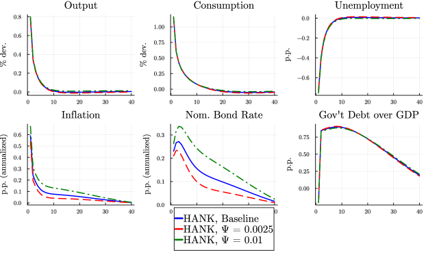
Figure 11: Model IRFs to stimulus checks by $\Psi$

Figure 11 displays the equivalent to Figure 9 in the main text. While all the responses are more short-lived due to the one-time nature of the shock, we still clearly see that $\Psi$ and thus the pressure of public debt on the “neutral” liquid rate matters for the inflation dynamics in its aftermath.

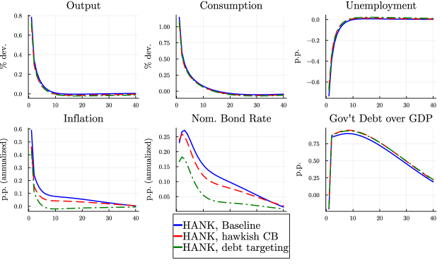
Figure 12: Model IRFs to stimulus checks by $\Psi$

Similarly, Figure 12 reveals the debt-targeting rule to provide for a particular fast disinflation after the shock without imposing substantial real costs.

Appendix D Additional Figures

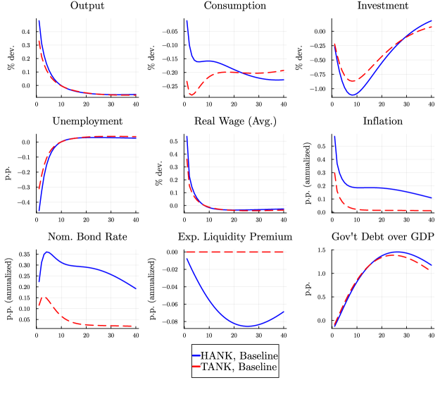
Figure 14: Model IRFs to Government Spending shock

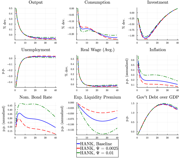
Figure 15: Model IRFs to gov’t spending shock for different $\Psi$

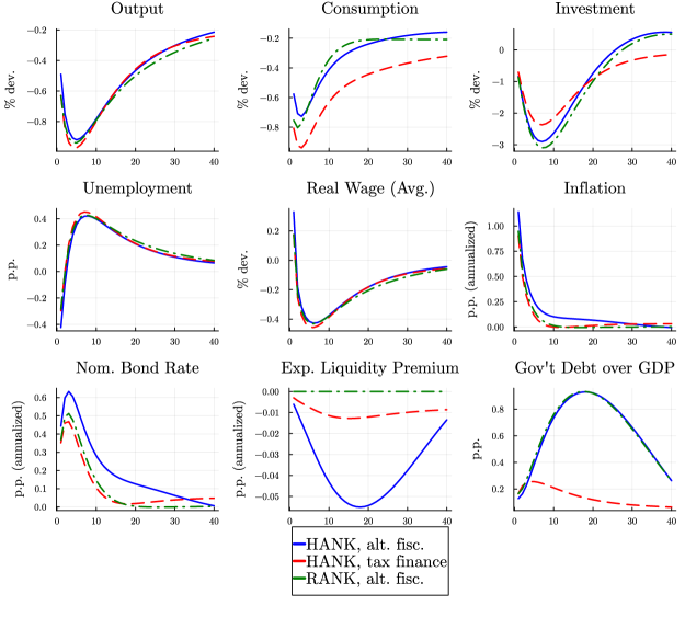
Figure 17: Model IRFs to TFP shocks for different fiscal policy rule

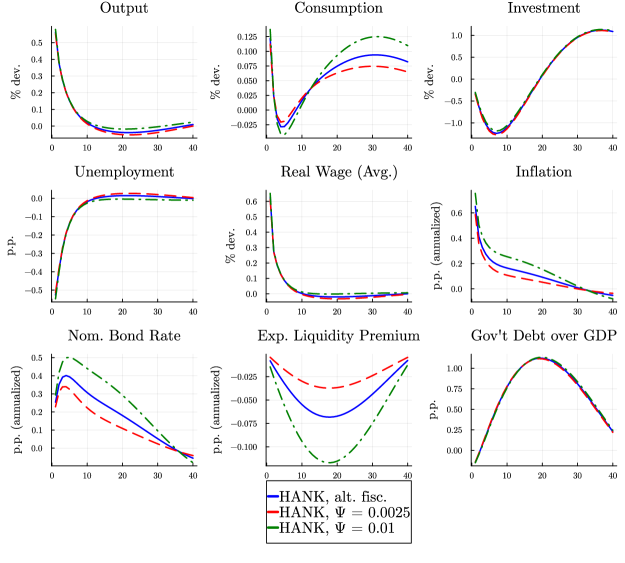
Figure 18: Model IRFs to gov’t spending shock for different fiscal policy rule

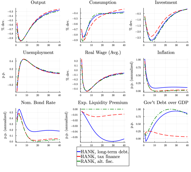
Figure 19: Model IRFs to TFP shocks under long-term debt

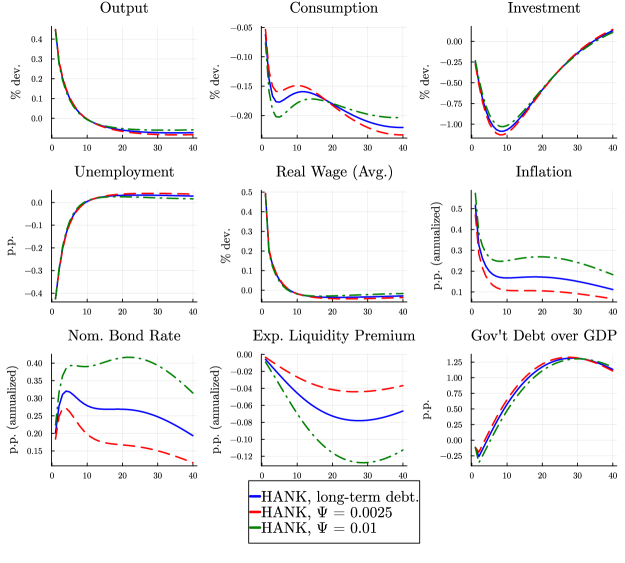
Figure 20: Model IRFs to gov’t spending shock under long-term deb

Figure 23: Model IRFs to TFP shocks for different policy rules

Figure 24: Model IRFs to gov’t spending shock for different policy rules

References

- Aguiar et al. (2023) Aguiar, M. A., M. Amador, and C. Arellano (2023): “Pareto Improving Fiscal and Monetary Policies: Samuelson in the New Keynesian Model,” Working Paper 31297, National Bureau of Economic Research.
- Amiti et al. (2023) Amiti, M., S. Heise, F. Karahan, and A. Şahin (2023): “Inflation Strikes Back: The Role of Import Competition and the Labor Market,” in NBER Macroeconomics Annual 2023, volume 38, University of Chicago Press.
- Ascari and Rankin (2013) Ascari, G. and N. Rankin (2013): “The effectiveness of government debt for demand management: Sensitivity to monetary policy rules,” Journal of Economic Dynamics and Control, 37, 1544–1566.
- Auclert et al. (2020) Auclert, A., M. Rognlie, and L. Straub (2020): “Micro Jumps, Macro Humps: Monetary Policy and Business Cycles in an Estimated HANK Model,” Working Paper 26647, National Bureau of Economic Research.
- Auclert et al. (2023) ——— (2023): “The Intertemporal Keynesian Cross,” Working paper, Harvard University.
- Bayer et al. (2023a) Bayer, C., B. Born, and R. Luetticke (2023a): “The liquidity channel of fiscal policy,” Journal of Monetary Economics, 134, 86–117.
- Bayer et al. (forthcoming) ——— (forthcoming): “Shocks, Frictions, and Inequality in US Business Cycles,” American Economic Review.
- Bayer et al. (2023b) Bayer, C., B. Born, R. Luetticke, and G. J. Müller (2023b): “The Coronavirus Stimulus Package: How large is the transfer multiplier?” Economic Journal, 133, 1318––1347.
- Bayer and Luetticke (2020) Bayer, C. and R. Luetticke (2020): “Solving discrete time heterogeneous agent models with aggregate risk and many idiosyncratic states by perturbation,” Quantitative Economics, 11, 1253–1288.
- Bayer et al. (2019) Bayer, C., R. Luetticke, L. Pham-Dao, and V. Tjaden (2019): “Precautionary Savings, Illiquid Assets, and the Aggregate Consequences of Shocks to Household Income Risk,” Econometrica, 87, 255–290.
- Bianchi et al. (2023) Bianchi, F., R. Faccini, and L. Melosi (2023): “A Fiscal Theory of Persistent Inflation*,” The Quarterly Journal of Economics, qjad027.
- Birinci and See (2021) Birinci, S. and K. See (2021): “Labor Market Responses to Unemployment Insurance: The Role of Heterogeneity,” Working Papers 2019-022, Federal Reserve Bank of St. Louis.
- Braxton et al. (2021) Braxton, J. C., K. F. Herkenhoff, J. L. Rothbaum, and L. Schmidt (2021): “Changing Income Risk across the US Skill Distribution: Evidence from a Generalized Kalman Filter,” Working Paper 29567, National Bureau of Economic Research.
- Broer et al. (2020) Broer, T., N.-J. H. Hansen, P. Krusell, and E. Öberg (2020): “The New Keynesian Transmission Mechanism: A Heterogeneous-Agent Perspective,” Review of Economic Studies, 87, 77–101.
- Calvo (1983) Calvo, G. A. (1983): “Staggered prices in a utility-maximizing framework,” Journal of Monetary Economics, 12, 383–398.
- Campos et al. (2024) Campos, R., J. Fernandez-Villaverde, G. Nuno, and P. Paz (2024): “Navigating by Falling Stars: Monetary Policy with Fiscally-driven Natural Rates,” Working paper, Bank of Spain.
- Carroll et al. (2017) Carroll, C., J. Slacalek, K. Tokuoka, and M. N. White (2017): “The distribution of wealth and the marginal propensity to consume,” Quantitative Economics, 8, 977–1020.
- Chiang and Żoch (2023) Chiang, Y.-T. and P. Żoch (2023): “Financial Intermediation and Aggregate Demand: A Sufficient Statistics Approach,” Working Papers 2022-038, Federal Reserve Bank of St. Louis.
- Christiano et al. (2016) Christiano, L. J., M. S. Eichenbaum, and M. Trabandt (2016): “UNEMPLOYMENT AND BUSINESS CYCLES,” Econometrica, 84, 1523–1569.
- Cochrane (2023) Cochrane, J. (2023): The Fiscal Theory of the Price Level, Princeton University Press.
- Consolo and Hänsel (2023) Consolo, A. and M. Hänsel (2023): “HANK faces unemployment,” Unpublished manuscript, Stockholm School of Economics.
- de Soyres et al. (2022) de Soyres, F., A. M. Santacreu, and H. L. Young (2022): “Fiscal policy and excess inflation during Covid-19: a cross-country view,” FEDS Notes 2022-07-15-1, Board of Governors of the Federal Reserve System (U.S.).
- Debortoli and Galí (2017) Debortoli, D. and J. Galí (2017): “Monetary policy with heterogeneous agents: Insights from TANK models,” Economics Working Papers 1686, Department of Economics and Business, Universitat Pompeu Fabra.
- den Haan et al. (2000) den Haan, W. J., G. Ramey, and J. Watson (2000): “Job Destruction and Propagation of Shocks,” American Economic Review, 90, 482–498.
- Dominguez Diaz (2021) Dominguez Diaz, R. (2021): “Precautionary Savings and Financial Frictions,” Job market paper, University of Bonn.
- Engen and Hubbard (2005) Engen, E. M. and R. G. Hubbard (2005): Federal Government Debt and Interest Rates, MIT Press, 83–160.
- Galí (2015) Galí, J. (2015): Monetary Policy, Inflation, and the Business Cycle: An Introduction to the New Keynesian Framework and Its Applications Second edition, no. 10495 in Economics Books, Princeton University Press.
- Gornemann et al. (2021) Gornemann, N., K. Kuester, and M. Nakajima (2021): “Doves for the Rich, Hawks for the Poor? Distributional Consequences of Monetary Policy,” Institute Working Paper 50, FRB Minneapolis Opportunity and Inclusive Growth Institute (OIGI).
- Graves (2021) Graves, S. (2021): “Does Unemployment Risk Affect Business Cycle Dynamics?” Working paper, Federal Reserve Board.
- Hagedorn et al. (2019) Hagedorn, M., I. Manovskii, and K. Mitman (2019): “The Fiscal Multiplier,” Working Paper 25571, National Bureau of Economic Research.
- Jorda et al. (2019) Jorda, O., K. Knoll, D. Kuvshinov, M. Schularick, and A. M. Taylor (2019): “The Rate of Return on Everything, 1870–2015,” The Quarterly Journal of Economics, 134, 1225–1298.
- Jordà and Nechio (2023) Jordà, O. and F. Nechio (2023): “Inflation and wage growth since the pandemic,” European Economic Review, 156, 104474.
- Jorda et al. (2017) Jorda, O., M. Schularick, and A. Taylor (2017): “Macrofinancial History and the New Business Cycle Facts,” NBER Macroeconomics Annual, 31, 213 – 263.
- Kaplan et al. (2018) Kaplan, G., B. Moll, and G. L. Violante (2018): “Monetary Policy According to HANK,” American Economic Review, 108, 697–743.
- Kaplan et al. (2023) Kaplan, G., G. Nikolakoudis, and G. L. Violante (2023): “Price Level and Inflation Dynamics in Heterogeneous Agent Economies,” Working Paper 31433, National Bureau of Economic Research.
- Kaplan and Violante (2018) Kaplan, G. and G. L. Violante (2018): “Microeconomic Heterogeneity and Macroeconomic Shocks,” Journal of Economic Perspectives, 32, 167–94.
- Kaplan et al. (2014) Kaplan, G., G. L. Violante, and J. Weidner (2014): “The Wealthy Hand-to-Mouth,” Brookings Papers on Economic Activity, 45, 77–153.
- Kekre (2022) Kekre, R. (2022): “Unemployment Insurance in Macroeconomic Stabilization,” The Review of Economic Studies, 90, 2439–2480.
- Klein (2000) Klein, P. (2000): “Using the generalized Schur form to solve a multivariate linear rational expectations model,” Journal of Economic Dynamics and Control, 24, 1405–1423.
- Krishnamurthy and Vissing-Jorgensen (2012) Krishnamurthy, A. and A. Vissing-Jorgensen (2012): “The Aggregate Demand for Treasury Debt,” Journal of Political Economy, 120, 233 – 267.
- Krueger et al. (2016) Krueger, D., K. Mitman, and F. Perri (2016): “Macroeconomics and Household Heterogeneity,” in Handbook of Macroeconomics, Elsevier, vol. 2, chap. Chapter 11, 843–921.
- Laubach (2009) Laubach, T. (2009): “New Evidence on the Interest Rate Effects of Budget Deficits and Debt,” Journal of the European Economic Association, 7, 858–885.
- Lee (2021) Lee, D. (2021): “The Effects of Monetary Policy on Consumption and Inequality,” Working paper, Federal Reserve Bank of New York.
- Leeper (1991) Leeper, E. (1991): “Equilibria under ’active’ and ’passive’ monetary and fiscal policies,” Journal of Monetary Economics, 27, 129–147.
- Leeper and Leith (2016) Leeper, E. and C. Leith (2016): “Understanding Inflation as a Joint Monetary & Fiscal Phenomenon,” in Handbook of Macroeconomics, Elsevier, vol. 2, chap. Chapter 30, 2305–2415.
- Ljungqvist and Sargent (2021) Ljungqvist, L. and T. Sargent (2021): “The fundamental surplus strikes again,” Review of Economic Dynamics, 41, 38–51.
- Niepelt (2004) Niepelt, D. (2004): “The Fiscal Myth of the Price Level,” The Quarterly Journal of Economics, 119, 277–300.
- Petrongolo and Pissarides (2001) Petrongolo, B. and C. A. Pissarides (2001): “Looking into the Black Box: A Survey of the Matching Function,” Journal of Economic Literature, 39, 390–431.
- Powell (2022) Powell, J. (2022): “Transcript of Chair Powell’s Press Conference June 15, 2022,” .
- Rachel and Summers (2019) Rachel, L. and L. H. Summers (2019): “On Secular Stagnation in the Industrialized World,” Brookings Papers on Economic Activity, 50, 1–76.
- Ramey (2016) Ramey, V. (2016): “Macroeconomic Shocks and Their Propagation,” in Handbook of Macroeconomics, Elsevier, vol. 2, chap. Chapter 2, 71–162.
- Ravn and Sterk (2017) Ravn, M. and V. Sterk (2017): “Job uncertainty and deep recessions,” Journal of Monetary Economics, 90, 125–141.
- Rotemberg (1982) Rotemberg, J. J. (1982): “Sticky Prices in the United States,” Journal of Political Economy, 90, 1187–1211.
- Sargent and Wallace (1981) Sargent, T. J. and N. Wallace (1981): “Some unpleasant monetarist arithmetic,” Quarterly Review, 5.
- Schmitt-Grohe and Uribe (2004) Schmitt-Grohe, S. and M. Uribe (2004): “Solving dynamic general equilibrium models using a second-order approximation to the policy function,” Journal of Economic Dynamics and Control, 28, 755–775.
- Schnabel (2022) Schnabel, I. (2022): “Finding the right mix: monetary-fiscal interaction at times of high inflation,” Keynote speech at the Bank of England Watchers’ Conference.
- Schnabel (2023) ——— (2023): “The last mile,” Keynote speech at the Homer Jones Memorial Lecture.
- Seidl and Seyrich (2023) Seidl, H. and F. Seyrich (2023): “Unconventional Fiscal Policy in a Heterogeneous-Agent New Keynesian Model,” Journal of Political Economy Macroeconomics, 1, 633–664.
- Shimer (2005) Shimer, R. (2005): “The Cyclical Behavior of Equilibrium Unemployment and Vacancies,” American Economic Review, 95, 25–49.
- Woodford (2001) Woodford, M. (2001): “Fiscal Requirements for Price Stability,” Journal of Money, Credit and Banking, 33, 669–728.
- Young (2010) Young, E. R. (2010): “Solving the incomplete markets model with aggregate uncertainty using the Krusell-Smith algorithm and non-stochastic simulations,” Journal of Economic Dynamics and Control, 34, 36–41.