Validation of ML-UQ calibration statistics using simulated reference values: a sensitivity analysis

Abstract

Some popular Machine Learning Uncertainty Quantification (ML-UQ) calibration statistics do not have predefined reference values and are mostly used in comparative studies. In consequence, calibration is almost never validated and the diagnostic is left to the appreciation of the reader. Simulated reference values, based on synthetic calibrated datasets derived from actual uncertainties, have been proposed to palliate this problem. As the generative probability distribution for the simulation of synthetic errors is often not constrained, the sensitivity of simulated reference values to the choice of generative distribution might be problematic, shedding a doubt on the calibration diagnostic. This study explores various facets of this problem, and shows that some statistics are excessively sensitive to the choice of generative distribution to be used for validation when the generative distribution is unknown. This is the case, for instance, of the correlation coefficient between absolute errors and uncertainties (CC) and of the expected normalized calibration error (ENCE). A robust validation workflow to deal with simulated reference values is proposed.

I Introduction

Most calibration statistics are used to compare UQ methods or datasets but are missing a reference value for validation. For instance, the correlation coefficient between absolute errors and uncertainties(Tynes2021, ) should be positive, but has no predefined reference value to compare with(Pernot2022b, ). This is also the case for some conditional calibration statistics, such as the expected normalized calibration error (ENCE)(Levi2022, ), which value depends moreover on the binning scheme(Pernot2023a_arXiv, ).

The use of probabilistic(Pernot2022c, ) or simulated(Rasmussen2023, ) reference values has been recently proposed to palliate the absence of reference value for a calibration statistic. A simulated reference value is estimated by applying the statistic to synthetic datasets containing the actual uncertainties and simulated errors generated from the uncertainties using a model generative distribution $D$.

The main issue with simulated references is the choice of $D$. Some calibration statistics depend explicitly on $D$ (typically a normal distribution): calibration curves and calibration error(Tran2020, ), negative log-likelihood (NLL)… This scenario fixes the choice of $D$ to simulate a reference value. However, this is not the case for many other calibration statistics, such as the calibration error, confidence curves(Pernot2022c, ) or reliability diagrams/ENCE(Pernot2023a_arXiv, ). Without constraint on $D$, the question arises of the sensitivity of such simulated reference values to the choice of generative distribution.

The case of confidence curves(Pernot2022c, ) enables to underline the main targets of the present study. A confidence curve is obtained by estimating an error statistic (e.g. the mean absolute error, MAE) for a dataset iteratively pruned from its largest uncertainties. Plotted against the percentage of pruned data, the confidence curve tests how the largest errors are associated with the largest uncertainties. Ideally, a confidence curve should be monotonously decreasing, but there is no predefined reference curve to assess its quality (the so-called oracle is unreachable in ML regression tasks(Pernot2022c, )). In this context, a confidence curve can inform us on the quality of the link between errors and uncertainties, but not on calibration. Using a simulated reference curve can solve this problem, at the cost of a choice for the generative distribution $D$, about which Pernot(Pernot2022c, ) has raised two main points:

• the sensitivity of the simulated reference curve to $D$ depends on the error statistic used to build the confidence curve: the MAE is very sensitive to $D$, while the root mean-squared error (RMSE) is not;

• for validation, a confidence band can be estimated from simulated reference curves. For all error statistics, the width of the confidence band depends on $D$, leading to ambiguous diagnostics when $D$ is not constrained.

The present study considers these two points for other calibration statistics. More specifically, it aims to test how simulated reference values for calibration statistics are sensitive to the choice of a generative distribution, how this impacts the validation procedure, and whether the uncertainty on the simulated reference value is a good choice of metric for validation. The focus is limited to statistics linked to ML regression tasks: the correlation coefficient between absolute errors and uncertainties (CC), an average calibration statistic (the mean squared z-scores, ZMS), and two conditional calibration statistics (the ENCE, its ZMS-derived analog ZMSE).

The next section defines the calibration statistics, the validation approach, and proposes a workflow dealing with the main issues of simulated references. Sect. III presents the application of these methods to an ensemble of nine datasets issued from the ML-UQ literature. The article proceeds with a discussion of the main findings (Sect. IV), and the conclusions are reported in Sect. V.

II Validation scores for calibration and correlation statistics

This section presents the simulation method for the estimation of calibration statistics references for commonly used correlation, average calibration and conditional calibration statistics in order to define adequate methods for their validation.

II.1 Probabilistic generative model

Let us consider a dataset composed of paired errors and uncertainties $\left\{E_{i},u_{E_{i}}\right\}_{i=1}^{M}$ to be tested for calibration. A few variance-based UQ validation statistics and methods, based on the correlation between the absolute errors and uncertainties (rank correlation coefficient (Sect. II.2) and confidence curve), avoid the need of a probabilistic model linking those variables(Pernot2022b, ). In contrast, most of the variance-based UQ calibration statistics are built implicitly on a probabilistic model

$$E_{i}\sim D(\mu=0,\sigma=u_{E_{i}})$$ (1)

or, equivalently,

$$E_{i}=u_{E_{i}}\varepsilon_{i}$$ (2)

linking errors to uncertainties, where $\varepsilon_{i}$ is a random number with zero-centered and unit-variance probability density function [$\varepsilon\sim D(\mu=0,\sigma=1)$]. This model states that errors should be unbiased ($\mu=0$) and that uncertainty quantifies the dispersion of errors, according to the metrological definition.(GUM, )

Except in some instances where $D$ is constrained by the method used to generate the dataset (gaussian process, normal likelihood models…), the shape of $D$ is unknown. This is notably the case when uncertainties are obtained by post-hoc calibration(Levi2022, ; Busk2022, ).

Note that $D$ should not be mistaken for the distribution of errors, which is a compound distribution between $D$ and the distribution of uncertainties. Let us assume that the errors are drawn from a distribution $D$ (Eq. 1) with a scale parameter $\sigma$ distributed according to a distribution $G$. The distribution of errors, H, is then a scale mixture distribution with probability density function

$$p_{H}(E)={\displaystyle\int_{0}^{\infty}p_{D}(E|\sigma)\,p_{G}(\sigma)\thinspace d\sigma}$$ (3)

Example - the NIG distribution. For a normal distribution $D=N(0,\sigma)$ and a distribution of variances described by an inverse gamma distribution $\sigma^{2}\sim IG(\frac{\nu}{2},\frac{\nu}{2})$, the compound distribution $H$ is a Student’s-t distribution with $\nu$ degrees of freedom, noted $t(\nu)$. This is a special case of the so-called Normal Inverse Gamma (NIG) distribution used, for instance, in evidential inference(Amini2019, ). $\oblong$

When $D$ is unknown, there is no evidence that it should be uniform across data space. To avoid unlimited complexity, this hypothesis will be made in the following, without affecting the main conclusions of the study.

II.2 Calibration statistics derived from the generative model

The generative model described above can be used to derive two families of calibration statistics.

II.2.1 The calibration error and related statistics.

The variance of the compound distribution of errors is obtained by the law of total variance, i.e.

$$\mathrm{Var}_{H}(E) =\left\langle\mathrm{Var}_{D}(E|\sigma)\right\rangle_{G}+\mathrm{Var}_{G}\left(\left\langle E|\sigma\right\rangle_{D}\right)$$ (4)

$$=<u_{E}^{2}>+\mathrm{Var}_{G}\left(\left\langle E|\sigma\right\rangle_{D}\right)$$ (5)

where the first term of the RHS has been identified as the mean squared uncertainty $<u_{E}^{2}>$. This expression can be compared to the standard expression for the variance

$$\mathrm{Var}(E) =<E^{2}>-<E>^{2}$$ (6)

For an unbiased error distribution, one gets $\mathrm{Var}_{G}\left(\left\langle E|\sigma\right\rangle_{D}\right)=0$ and $<E>=0$, leading to

$$<E^{2}>=<u_{E}^{2}>$$ (7)

on which some popular calibration statistics are based.

Example, followed. Considering the NIG model, one can easily verify from the properties of the Student’s-t distribution that

$$<E^{2}>=\sigma^{2}\nu/(\nu-2)$$ (8)

(using $<E>=0$), and from the inverse gamma distribution(Evans2000, ) that

$$<u_{E}^{2}>=\sigma^{2}\nu/(\nu-2)$$ (9)

so that Eq. 7 is fulfilled. $\oblong$

Based on Eq. 7, the Relative Calibration Error is defined as

$$RCE=\frac{RMV-RMSE}{RMV}$$ (10)

where $RMSE$ is the root mean squared error $\sqrt{<E^{2}>}$ and $RMV$ is the root mean variance ($\sqrt{<u_{E}^{2}>}$). The RCE has been shown to be very sensitive to the upper tail of the uncertainty distribution and to become unreliable for a large portion of the studied ML-UQ datasets(Pernot2024_arXiv, ). It is therefore not considered directly here, but it is used in a bin-based statistic of conditional calibration, the Expected Normalized Calibration Error(Levi2022, )

$$ENCE=\frac{1}{N}\sum_{i=1}^{N}|RCE_{i}|$$ (11)

where $RCE_{i}$ is estimated over the data within bin $i$.

Pernot(Pernot2023a_arXiv, ) has shown that the ENCE reference value is not zero, and that it depends on the binning scheme. As demonstrated in Appendix B, the ENCE depends on both the dataset size and the number of bins and does not have a predefined reference value.

According to the binning variable, the ENCE might be used to test consistency (binning on $u_{E}$) or adaptivity (binning on input features).(Pernot2023d, ) Because of the limited range of each bin, the ENCE is not expected to suffer from the same problem as the RCE when the binning variable is the uncertainty.

II.2.2 The ZMS and related statistics.

Another approach to calibration based on Eq. 1 uses scaled errors or z-scores

$$Z_{i}=\frac{E_{i}}{u_{E_{i}}}\sim D(0,1)$$ (12)

with the property

$$Var(Z)=1$$ (13)

assessing average calibration for unbiased errors(Pernot2022a, ; Pernot2022b, ). For biased errors, the calibration equation becomes

$$ZMS=<Z^{2}>=1$$ (14)

which is the preferred form for testing(Pernot2023d, ) (ZMS stands for z-score’s mean squares). This choice is motivated by the use of the ZMS for binned data, where, even for an unbiased dataset, one should not expect every bin to be unbiased. The ZMS does not depend on a distribution hypothesis and its target value is 1.

The negative log-likelihood (NLL) score can be written as(Busk2023, )

$$NLL =\frac{1}{2}\left(<Z^{2}>+<\ln u_{E}^{2}>+\ln 2\pi\right)$$ (15)

It combines an average calibration term, the ZMS,(Zhang2023, ) and a sharpness term driving the uncertainties towards small values(Gneiting2007a, ) when the NLL is used as a loss function, hence preventing the minimization of $<Z^{2}>$ by arbitrary large uncertainties. The NLL is the logarithm of a normal probability density function and therefore should be used only when the errors and uncertainties are linked by a standard normal generative distribution ($D=N(0,1)$). Knowing the reference value of $<Z^{2}>$, one can assign a reference value to the NLL

$$NLL_{ref}=\frac{1}{2}\left(1+<\ln u_{E}^{2}>+\ln 2\pi\right)$$ (16)

Note that Rasmussen et al.(Rasmussen2023, ) threat the NLL as if it had no predefined reference value and needed a simulated reference. This is not the case when the NLL is defined by Eq. 15, but it might be for other likelihood definitions. In the present case, for a given set of uncertainties, validation of the NLL is equivalent to the validation of the ZMS, with the additional constraint of a normal generative model.

By analogy with the ENCE, one can define a ZMS-based mean calibration error(Pernot2023c_arXiv, )

$$ZMSE=\frac{1}{N}\sum_{i=1}^{N}|\ln ZMS_{i}|$$ (17)

where $i$ runs over the $N$ bins and $ZMS_{i}$ is estimated with the data in bin $i$. The logarithm accounts for the fact that ZMS is a scale statistic (a ZMS of 2 entails a deviation of the same amplitude as a ZMS of 0.5). As for the ENCE, the ZMSE measures conditional calibration, i.e. consistency if the binning variable is the uncertainty or adaptivity if it is an input feature. Also, ZMSE depends on the dataset size and bin number (Appendix B), and doe not have a predefined reference value. As observed for the ZVE defined by Pernot(Pernot2023a_arXiv, ), one might expect the ZMSE to be more reliable than the ENCE for heavy-tailed uncertainty distributions.

II.3 Correlation

The correlation between absolute errors and uncertainties

$$CC=\mathrm{cor}(|E|,u_{E})$$ (18)

is used to assess the strength of the link between these variables(Tynes2021, ). One expects large absolute errors to be associated with large uncertainties and small uncertainties to be associated with small absolute errors. However, the link is not symmetric, as small absolute errors might be associated with large uncertainties. To account for a possible non linear relation and to reduce the sensitivity to outliers, Spearman’s rank correlation coefficient is recommended to estimate CC.

A positive value of CC is desirable, but, considering the probabilistic link between errors and uncertainties, its reference value cannot be 1.(Pernot2022b, ) In absence of a specified target value, the CC alone should not be used in comparative studies, nor for validation.

II.4 Validation

The validation protocol has been presented in Ref(Pernot2024_arXiv, ). The main points are summarized here. For a given dataset $(E,u_{E})$ and statistic $\vartheta$, one estimates the statistic over the dataset $\vartheta_{est}$ and a 95 % confidence interval $I_{BS}=\left[I_{BS}^{-},I_{BS}^{+}\right]$ by bootstrapping using the Bias Corrected Accelerated (BC_a) method(DiCiccio1996, ). One can then test that the target value for the statistic, $\vartheta_{ref}$, lies within $I_{BS}$, i.e.

$$\vartheta_{ref}\in\left[I_{BS}^{-},I_{BS}^{+}\right]$$ (19)

For a non-binary agreement measure, a standardized score $\zeta$ is defined as

$$\zeta(\vartheta_{est},\vartheta_{ref},I)=\begin{cases}\frac{\vartheta_{est}-\vartheta_{ref}}{I_{BS}^{+}-\vartheta_{est}}&if\,(\vartheta_{est}-\vartheta_{ref})\leq 0\\ \frac{\vartheta_{est}-\vartheta_{ref}}{\vartheta_{est}-I_{BS}^{-}}&if\,(\vartheta_{est}-\vartheta_{ref})>0\end{cases}$$ (20)

that can be tested by

$$|\zeta|\leq 1$$ (21)

which is strictly equivalent to the interval test (Eq. 19). In addition, $\zeta$ provides valuable information about the sign and amplitude of the agreement between the statistic and its reference value.

The validation procedure depends then on the availability of $\vartheta_{ref}$, as shown next.

II.4.1 Predefined $\vartheta_{ref}$

If $\vartheta_{ref}$ is known, one can directly use Eq. 20 to estimate

$$\zeta_{BS}=\zeta(\vartheta_{est},\vartheta_{ref},I_{BS})$$ (22)

which will be considered below as the benchmark method against which the alternative simulation-based methods will be evaluated.

II.4.2 Estimation of $\vartheta_{ref}$ by simulation

For those statistics without a predefined reference value, one has to make an hypothesis on $D$, in order to generate $\vartheta_{ref}$ from ideally calibrated datasets:

1. Choose a unit-variance generative distribution $D(0,1)$.

2. Draw a set of pseudo-errors from the actual uncertainties by applying Eq. 1 and estimate the corresponding statistic $\tilde{\vartheta}_{D}$, where the subscript $D$ denotes the choice of generative distribution.

3. Repeat step 2 $N_{MC}$ times (Monte Carlo sampling).

4. Take the mean value $\tilde{\vartheta}_{D,ref}=<\tilde{\vartheta}_{D}>$ and estimate the standard error on $\tilde{\vartheta}_{D,ref}$: $u(\tilde{\vartheta}_{D,ref})=\mathrm{sd}(\tilde{\vartheta}_{D})/\sqrt{N_{MC}}$, where $\mathrm{sd}(x)$ is the standard deviation of variable $x$.

For $N_{MC}$ on the order of $10^{4}$, one should have $2u(\tilde{\vartheta}_{D,ref})\ll U_{BS}$, where $U_{BS}$ is the half range of $I_{BS}$, and Eq. 20 can be applied without accounting for the uncertainty on $\tilde{\vartheta}_{D,ref}$. One can then estimate a $\zeta$-score

$$\zeta_{SimD}=\zeta(\vartheta_{est},\tilde{\vartheta}_{D,ref},I_{BS})$$ (23)

Note that this approach differs from the one proposed previously in the literature(Pernot2022c, ; Rasmussen2023, ), where the value of the statistic was considered as fixed and the reference value as a random variable with uncertainty $\mathrm{sd}(\tilde{\vartheta}_{D})$. This scenario is implemented for comparison, with

$$\zeta_{Sim2D}=\zeta(\vartheta_{est},\tilde{\vartheta}_{D,ref},I_{D})$$ (24)

using a confidence interval $I_{D}$ estimated from the the quantiles of the simulated sample of $\tilde{\vartheta}_{D}$.

It is important to acknowledge that validation tests based on the latter approach present two drawbacks when compared to the bootstrapping-based procedure: (1) they ignore uncertainty on $\vartheta_{est}$, creating an asymmetric treatment of the statistics, depending on the existence or not of a known reference value; (2) the limits of the confidence interval $I_{D}$ can be very sensitive to the choice of generative distribution $D$,(Pernot2022c, ) as will be illustrated in Sect. III.

II.4.3 Recommended validation workflow

A recommended validation workflow for a given statistic $\vartheta$ is shown in Fig. 1. Note that it is essential that $\vartheta$ should be first confirmed as being fit to the purpose of the study, notably for datasets with highly skewed and/or heavy-tailed uncertainty distributions(Pernot2024_arXiv, ).

Figure 1: Flowchart for the validation of a statistic $\vartheta$. $\vartheta_{ref}$ is the reference value used for validation, $\vartheta_{est}$ is the actual value of the statistic, $I_{BS}$ is the bootstrapped CI for $\vartheta_{est}$ and $D$ is the error generative distribution.

For statistics with a known reference value, one can apply directly the benchmark method (Eq. 22). In the absence of a predefined reference value for a statistic, one might generate a simulated one (Sect. II.4.2), but a weak point of this method is that one has to choose a generative distribution $D$ linking the errors to the uncertainties (Eq. 1).

If $D$ is well constrained, one may proceed to the estimation of the simulated reference value $\tilde{\vartheta}_{D,ref}$ and use it for validation (Eq. 23). In absence of constraints on $D,$ it is essential to estimate the sensitivity of $\tilde{\vartheta}_{D,ref}$ to $D$. For this, at least two alternative shapes for $D$ have to be considered, for instance $D=N(0,1)$ and $D=t_{s}(\nu)$, the unit-variance Student’s-t distribution is defined as

$$t_{s}(\nu)=t(\nu)/\sqrt{\nu/(\nu-2)}$$ (25)

One should use a value of $\nu$ small enough to provide a contrast with the normal distribution, but not too small, as it might generate problematic error sets with many outliers. A value of $\nu=6$ is found as a good compromise in the following. If the simulated reference values for these choices of $D$ differ more than their statistical uncertainty, the statistic should not be used for validation. Otherwise, one might proceed as in the case of a predefined $D$ (Eq. 23).

III Applications

The validation approach presented above is applied to nine datasets extracted from the ML-UQ literature, with a focus on the shapes of the distributions of the errors, uncertainties and z-scores and their consequences for the validation process, followed by a thorough study of the sensitivity of the procedure to various parameters, such as the uncertainty distribution and the shape of the generative distribution.

III.1 The datasets

Nine test sets, including errors and calibrated uncertainties, have been taken from the recent ML-UQ literature for the prediction of various physico-chemical properties by a diverse panel of ML methods. The selection rejected small datasets and those presenting duplicated properties. Note these uncertainties have been calibrated by a palette of methods with various levels of success. The datasets names, sizes and bibliographic references are gathered in Table 1, and the reader is referred to the original articles for details. In the following, a short notation is used, e.g. ’Set 7’ corresponds to the QM9_E dataset.

Set #	Name	Size ($M$)		Reference
1	Diffusion_RF	2040		Palmer et al.(Palmer2022, )
2	Perovskite_RF	3834		Palmer et al.(Palmer2022, )
3	Diffusion_LR	2040		Palmer et al.(Palmer2022, )
4	Perovskite_LR	3836		Palmer et al.(Palmer2022, )
5	Diffusion_GPR_Bayesian	2040		Palmer et al.(Palmer2022, )
6	Perovskite_GPR_Bayesian	3818		Palmer et al.(Palmer2022, )
7	QM9_E	13885		Busk et al.(Busk2022, )
8	logP_10k_a_LS-GCN	5000		Rasmussen et al.(Rasmussen2023, )
9	logP_150k_LS-GCN	5000		Rasmussen et al.(Rasmussen2023, )

Table 1: The nine datasets used in this study: number, name, size and reference.

Those same datasets were tested by Pernot(Pernot2024_arXiv, ) for average calibration by the ZMS statistic and the result is reported in the first column of Table 2. Only four of the nine sets passed the test for average calibration (Sets 1, 6, 7 and 9). In the same study, it was shown that using the RCE statistic (Eq. 10) for average calibration testing was problematic, and notably that this statistic was unreliable for the sets marked as “Failed RCE” in Table 2 (Sets 2, 3, 4, 6 and 7). This issue was traced back to the high sensitivity of the root mean variance (RMV) involved in the RCE expression to the upper tail of the uncertainty distribution.

Set #	Calibrated	Failed RCE		$\beta_{GM}(u_{E})$		$k=\nu/2$		$\vartheta=\nu/2*\sigma^{2}$			$\nu=2k$		$\nu_{eff}$
1	$\checkmark$			0.172		-		-			-		-
2		$\checkmark$		0.419		-		-			-		-
3		$\checkmark$		0.485		4.	52	7.	32E-01		9.	04	6.	8
4		$\checkmark$		0.438		1.	57	2.	44E-01		3.	14	3.	3
5				0.113		21.	10	1.	82		42.	20	4.	0
6	$\checkmark$	$\checkmark$		-		-		-			-		-
7	$\checkmark$	$\checkmark$		0.524		1.	81	1.	72E-04		3.	61	2.	2
8				0.231		23.	40	1.	91		46.	80	3.	9
9	$\checkmark$			0.223		16.	90	3.	91E-01		33.	80	2.	9

Table 2: Tailedness of the uncertainty distributions: $\beta_{GM}$ skewness of the uncertainties and parameters of the fit of the squared uncertainties by $IG(k,\theta)$ distributions. $k$ is the shape parameter, assimilated to $\nu/2$ in the NIG model, and $\vartheta$ is the scale parameter, which absorbs the scale of $u_{E}^{2}$, noted $\sigma^{2}$. The missing values mark the sets with a bad fit by the $IG$ model or a non-representative $\beta_{GM}$. The values of the $\nu_{eff}$ parameters obtained from the fit of the errors distribution by the NIG model (Table 3) are reported for comparison with $\nu=2k$.

In order to have a clear view of the distributions involved in the generative model for the estimation of simulated references, the distributions of $u_{E,}$, $E$ and $Z$ for the nine datasets are characterized in the next sections.

III.1.1 Uncertainty distributions

Fig. 2 presents histograms of the logarithm of squared uncertainties for the nine datasets. $u_{E}^{2}$ has been fitted by an inverse gamma distribution $IG(k,\theta)$, to assess the pertinence of the NIG model defined above. The best fit curves are compared to the data histograms and show a reasonable agreement, except for Sets 1, 2 and 6. Uncertainties of Sets 1 appear to be bimodal, which cannot be modeled by the $IG$ distribution, while for Set 2, the $IG$ model is defeated by a long left tail of small uncertainties. Set 6 presents a combination of both features. The parameters of the fitted $IG(k,\theta$) distribution are reported in Table 2. One sees that if one excludes the problematic datasets, the shape parameter covers a large range, from 1.57 to 23.4, corresponding to skewness values varying from infinity to about 1 (skewness of the $IG$ distribution is not defined for $k\leq 3$).

Figure 2: Uncertainty distributions. The histograms of $log(u_{E}^{2})$ are compared to the fit of $u_{E}^{2}$ by an Inverse-Gamma distribution (blue line). The mean variance ($MV=<u_{E}^{2}>$) is marked by a red line and the median variance (MedV) by an orange line. The distance between $MV$ and $MedV$ characterizes the skewness of the distribution of squared uncertainties.

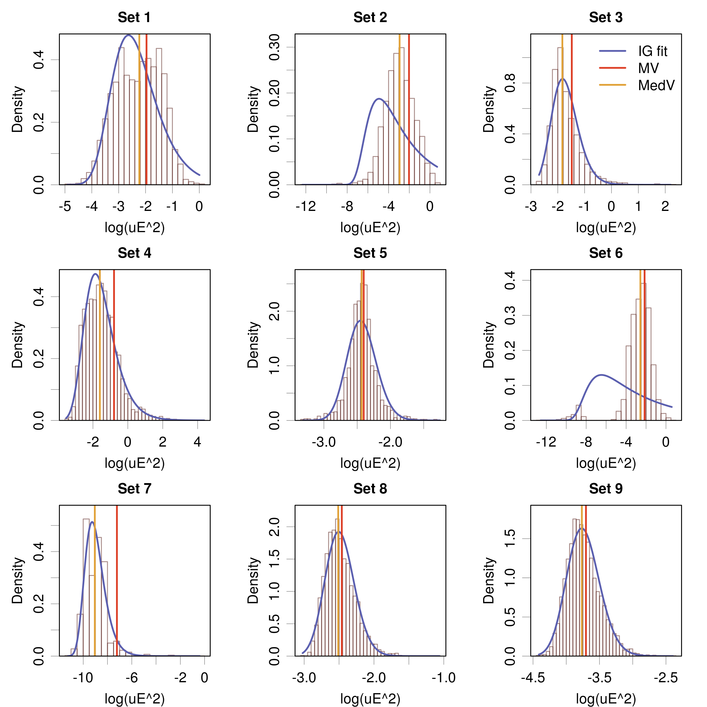
The mean variance and median variance were marked in Fig. 2. The distance between those values is an estimator of the skewness of the $u_{E}^{2}$ distribution. To be more quantitative and focus on the uncertainties instead of their square, skewness of the uncertainty distributions was quantified by $\beta_{GM}$, a skewness statistic robust to outliers based on the scaled difference between the mean and median (Groeneveld1984, ; Pernot2021, ). $\beta_{GM}$ varies between -1 and 1 and is null for symmetric distributions. One can see in Table 2 that all the datasets that challenge the RCE statistic have $\beta_{GM}$ values above 0.4, except for Set 6, for which skewness is not a pertinent descriptive statistic for such a bimodal distribution. One can see for the sets with a successful $IG$ fit that $\beta_{GM}$ is correctly anti-correlated to $k$.

III.1.2 Distributions of errors and z-scores

The distributions of errors $E$ and z-scores $Z$ are characterized to assess their shapes and departure from normality. Table 3 reports the mean values, standard deviations, relative bias and effective number of degrees of freedom $\nu_{eff}$ resulting from the fit of the data by a scaled and shifted Student’s-t distribution. The smaller $\nu_{eff}$, the farther one is from a normal distribution. This fit accounts for a possible bias in the dataset, which is non-negligible (above 5 % of the standard deviation) only for Sets 9 for E, and Sets 8 and 9 for Z. Figs 3-4 compare the fits of the errors and z-scores by normal and Student’s-t distributions.

Set #	$\mu_{E}$		$\sigma_{E}$		$b_{E}$ (%)	$\nu_{eff,E}$			$\mu_{Z}$		$\sigma_{Z}$		$b_{Z}$ (%)	$\nu_{eff,Z}$
1	0.	0033(81)	0.	3678(81)	1	3.	0		-0.	027(22)	0.	980(30)	3	6.	0
2	0.	0034(61)	0.	377(13)	1	1.	4		-0.	018(15)	0.	940(26)	2	3.	3
3	0.	008(11)	0.	4810(98)	2	6.	8		0.	002(23)	1.	058(18)	0	20.	1
4	0.	001(10)	0.	637(15)	0	3.	3		-0.	021(18)	1.	107(16)	2	9.	1
5	0.	0019(60)	0.	2713(61)	1	4.	0		0.	006(20)	0.	920(21)	1	3.	9
6	0.	0044(50)	0.	310(14)	1	1.	3		-0.	005(16)	0.	992(37)	1	1.	4
7	0.	00131(29)	0.	0341(48)	4	2.	2		0.	0174(84)	0.	9858(99)	2	4.	4
8	0.	0116(39)	0.	2786(52)	4	3.	9		0.	050(14)	0.	961(16)	5	3.	9
9	-0.	0424(22)	0.	1533(39)	28	2.	9		-0.	260(13)	0.	951(23)	27	3.	1

Table 3: Summary statistics for the errors ($E$) and z-scores ($Z$): $\mu_{X}$ is the mean value of variable $X$, $\sigma_{X}$ its standard deviation, $b_{X}=100(\mu_{X}-0)/\sigma_{X}$ measures relative bias and $\nu_{eff,X}$ is the number of degrees of freedom resulting from the fit of the data by a scaled and shifted Student’s-t distribution.

Figure 3: Error distributions (histograms) with normal (red line) and scaled and shifted Student’s-t (blue line) fits. For legibility, the histograms have been truncated to $\pm 3$ standard deviations, hiding a few outlying errors.

Figure 4: Same as Fig. 3 for z-scores.

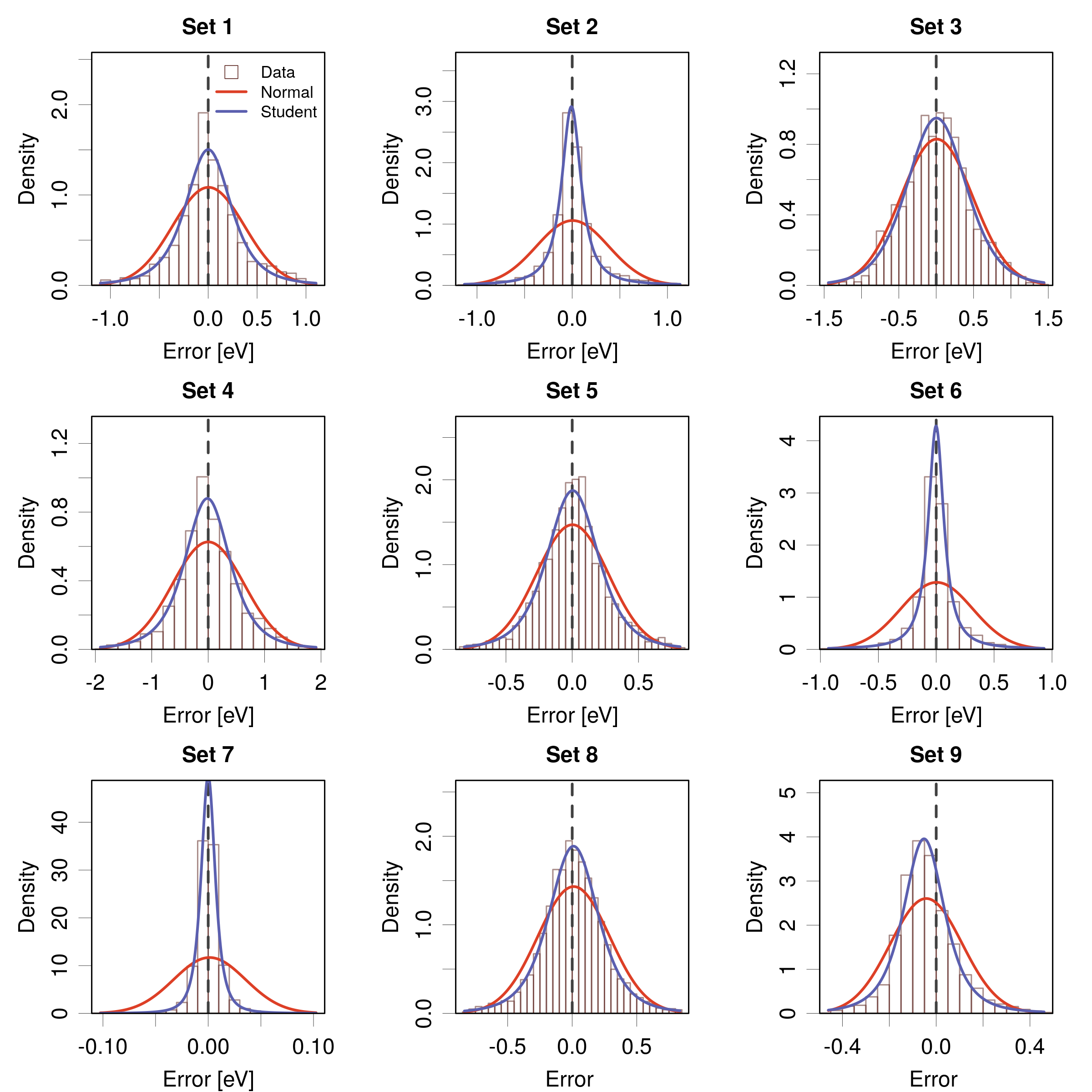
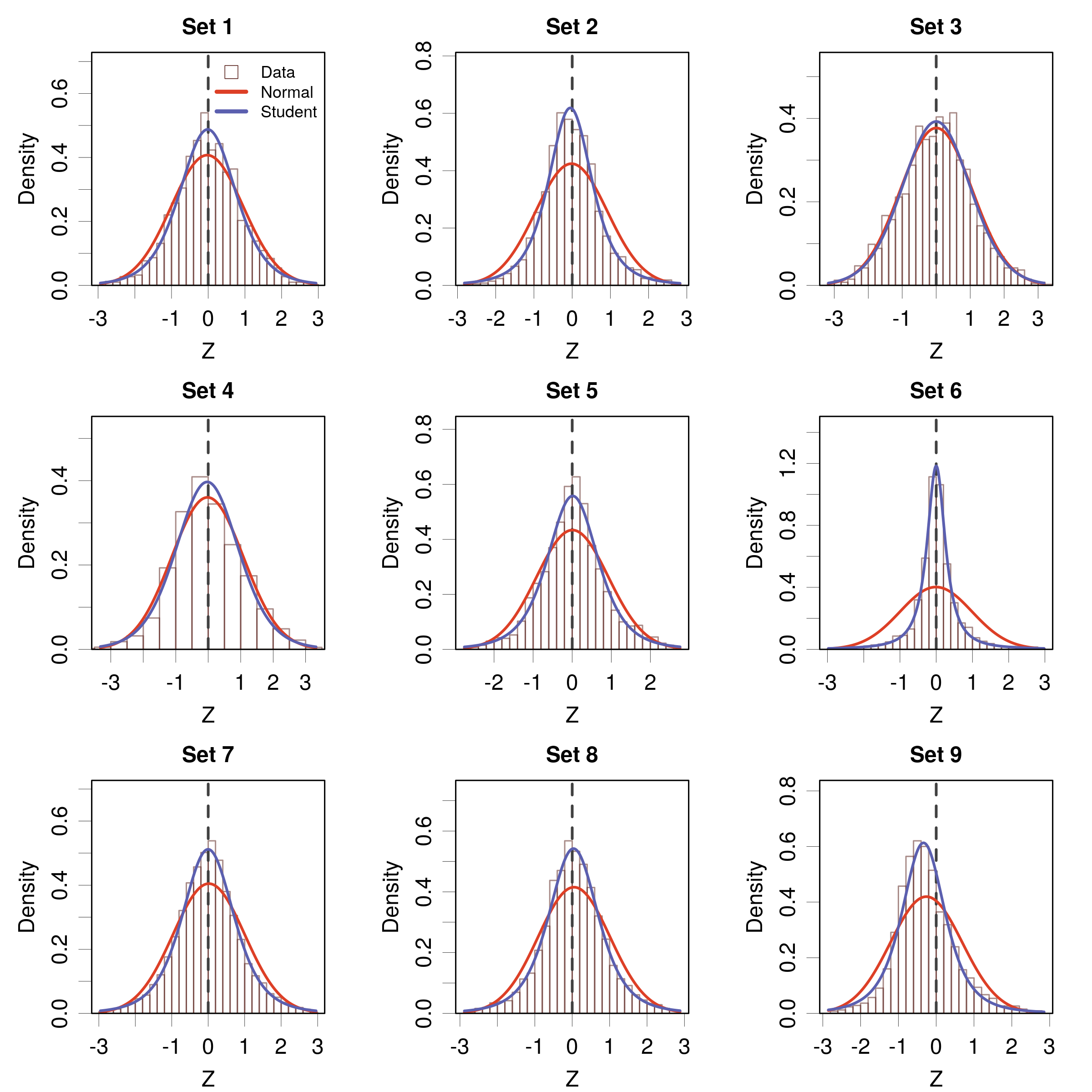
The histograms and $\nu_{eff}$ values indicate that none of the the error distributions is close to normal, which is a common feature of error distributions(Pernot2020b, ; Pernot2021, ), and is consistent with the generative model and the uncertainty distributions of these datasets (Table 2). The largest value of $\nu_{eff,E}$ is 6.8 for Set 3, which is still a rather small value (a normal distribution corresponds to $\nu_{eff}=+\infty$, but values above 20-30 could be considered as close-to-normal). One can note also that some values of $\nu_{eff,E}$ are smaller than 2 (for Sets 2 and 6), corresponding to Student’s-t distributions with infinite variance.

If one considers the z-scores, there is a notable trend for the values of $\nu_{eff}$ to be larger than their counterparts for the errors, except for a few sets (5, 6, 8) for which they are identical. The only set for which one gets notably closer to normality is Set 3, with $\nu_{eff,Z}=20.1$. Overall, one has still relatively small $\nu_{eff}$ values, rejecting the normality of z-scores for 8 out of nine datasets. Note that the normality of z-scores should not be used as a calibration criterion.

III.2 Analysis of the generative model

Having characterized the uncertainty and error distributions, one can put the generative model to the test and try to characterize the generative distribution $D$.

Non-normality of $D$.

In the hypothesis that the generative distribution $D$ is standard normal, one should have approximately $\nu_{eff}\simeq 2k$ (Table 2) for those sets with good $IG$ fits, where $\nu_{eff}$ was estimated for the error distributions (Table 3). This is the case for Set 4, and to a lesser extent for Set 7. On the contrary, Sets 5, 8 and 9 have very large shape parameters which contrast strongly with the small values of $\nu_{eff}$. Reasoning on the single calibrated dataset for which $k$ and $\nu_{eff}$ are available, i.e. Set 9, on should conclude on the non-normality of the generative distribution $D$, or at least that the normality of $D$ cannot be considered as a general hypothesis.

Using $Z$ distribution as a proxy for $D.$

Considering the generative model, the distribution of z-scores for a calibrated dataset should be identical to $D$. To check how close the distribution of z-scores is to the errors generative distribution, simulated error distributions have been generated using the actual uncertainties and two generative distributions: a standard Normal distribution $N(0,1)$ and a unit-variance Student’s-t distribution $t_{s}(\nu_{eff,Z})$ with the degrees of freedom estimated for $Z$ (Table 3). The results are shown in Fig. 5.

Figure 5: Recovery of the error distributions with the generative model, using a normal distribution (red line) and unit-variance Student’s-t with effective degrees of freedom for $Z$ (Table 3; blue line). For Set 6, the Student’s-t model cannot be generated because of the infinite variance for $\nu_{eff,Z}<2$ and it was replaced by $\nu_{eff,Z}=2.1$.

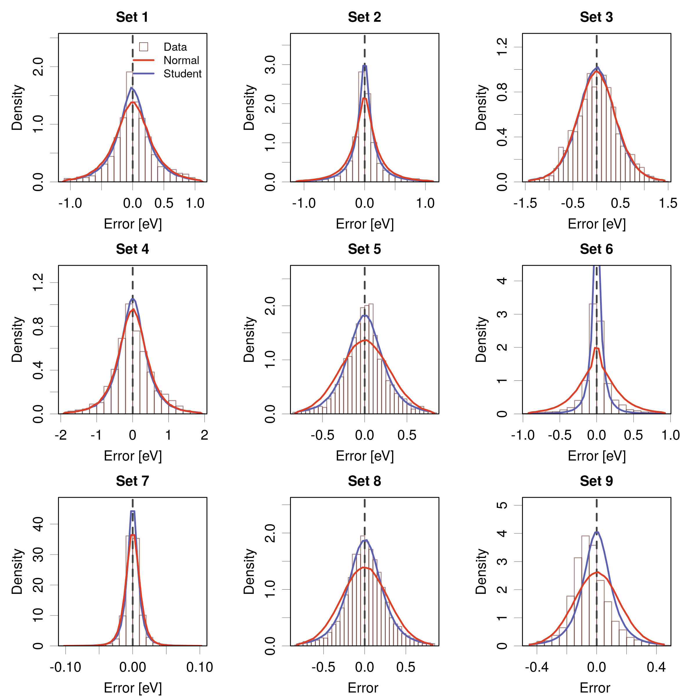
The $t_{s}$-based model offers a better fit to the errors histogram for Sets 2, 5, 6, 7, 8 and 9 (considering that Set 9 is affected by a notable bias of the errors). For the other sets, it is on par with the normal model. Note that for Set 6 the value of $\nu_{eff,Z}$ has been fixed to 2.1 to avoid the infinite variance caused by $\nu_{eff,Z}\leq 2$.

It is thus clear that a normal generative distribution $D=N(0,1)$ is not likely to provide simulated error distributions with properties close to the actual errors, except for a few datasets (Sets 1, 3 and 4). A Student’s-t model for the generative distribution $D=t_{s}(\nu_{eff,Z})$, based on the distribution of z-scores might thus offer an interesting alternative to the normal distribution for the generation of simulated error sets, and it might also be useful to test the sensitivity of simulated statistics to $D$, as tested thereafter.

III.3 Sensitivity analysis

In the previous section, we have seen that if there is a best choice for the generative distribution $D$, it is rarely the normal distribution, which leaves the question of its choice. In absence of strong constraints to guide this choice, it is important to assess the sensitivity to $D$ of the simulated reference values for the candidate calibration statistics, and more globally the sensitivity of the validation $\zeta$-scores.

III.3.1 Sensitivity of $\tilde{\vartheta}_{D,ref}$ to the uncertainty distribution

A first point is the appreciation of the dependence of the simulated reference values on the uncertainty distribution. For this, a normal generative distribution is chosen [$D=N(0,1)$], and $\tilde{\vartheta}_{D,ref}$ and $u(\tilde{\vartheta}_{D,ref})$ are estimated for each statistic and the nine example datasets. The sampling size is $N_{MC}=10^{4}$ and $u_{E}$ is sorted and parted into 50 equal-size bins to estimate the ENCE and ZMSE statistics. The results are presented in Fig. 6.

Figure 6: Sensitivity of $\tilde{\vartheta}_{D,ref}$ to the dataset for the ZMS (a), CC (b), ENCE (c, d) and ZMSE (e, f) statistics. The generative distribution is standard normal, $D=N(0,1)$.

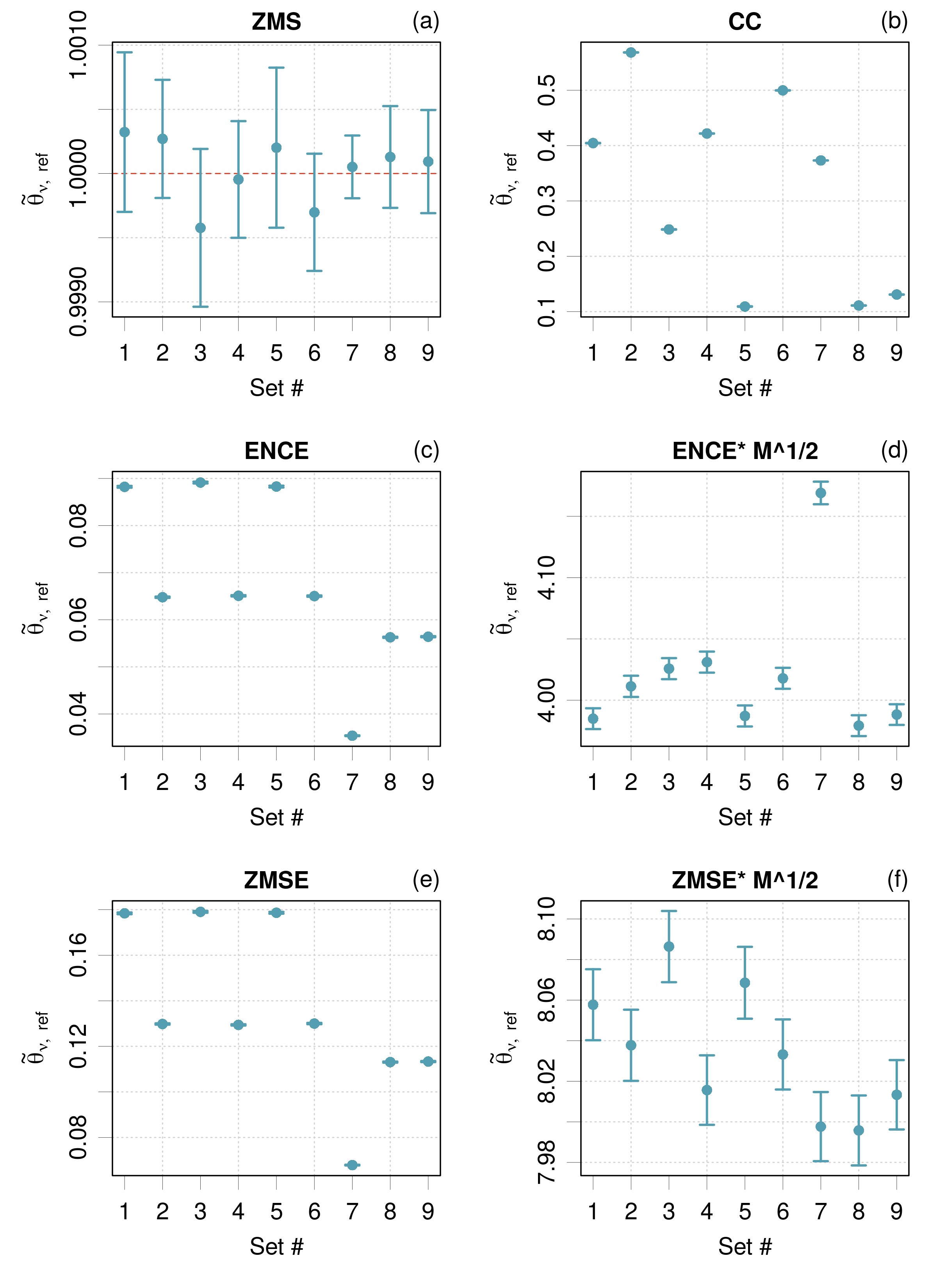
For ZMS [Fig. 6(a)], the simulation recovers correctly the predefined reference value, showing the consistency of the simulation approach for this statistic. For CC [Fig. 6(b)], $\tilde{\vartheta}_{D,ref}$ depends strongly on the dataset, confirming the absence of a common reference value for these datasets. The ENCE [Fig. 6(c)] and ZMSE [Fig. 6(e)] follow a parallel pattern, which is mostly due to the sensitivity of these variables to the dataset size, $M$ (Appendix B). The correction of this trend by multiplying by $M^{1/2}$ [Fig. 6(d,f)] shows that the common pattern disappears and that each uncertainty set leads to its own reference value, even if a few CIs overlap. The ENCE has an outstanding value of $\tilde{\vartheta}_{D,ref}$ for Set 7, which is not the case for ZMSE, and might be the manifestation of an over-sensitivity of the ENCE to features of the uncertainty distribution.

Globally, apart from the ZMS, on needs therefore to estimate a simulated reference value for each set and statistic.

III.3.2 Sensitivity of $\tilde{\vartheta}_{D,ref}$ to $D$

The simulated reference values are generated for Sets 7 and 8 (as representative of the largest sets with markedly different uncertainty distributions) from their actual uncertainties by using a unit-variance Student’s-t generative distribution $D=t_{s}(\nu)$ for a range of degrees of freedom between 3 and 20, covering the range of values observed for $\nu_{eff,Z}$ (Table 3). The sampling size is $N_{MC}=10^{4}$ and $u_{E}$ is sorted and parted into 50 equal-size bins to estimate the ENCE, ZMSE. The results are presented in Fig. 7.

Figure 7: Sensitivity of the simulated reference values to the generative distribution. Calibrated datasets are generated from the actual uncertainties of Sets 7 and 8, using a generative distribution $D=t_{s}(\nu)$ with $\nu$ degrees of freedom.

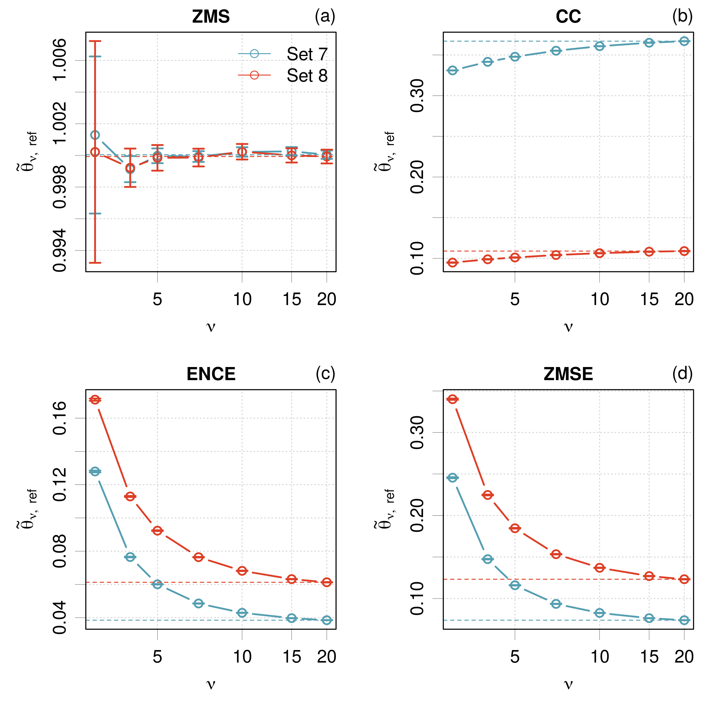
For ZMS [Fig. 7(a)], one expects to observe the conformity of the simulated reference value with the known reference value (i.e. $\tilde{\vartheta}_{\nu,ref}\simeq 1$), independently of the chosen generative distribution. This is the case, albeit with a notable increase of Monte Carlo sampling uncertainty as $v$ decreases. For CC [Fig. 7(b)], the sensibility to $\nu$ depends on the value of the statistic, and it is less marked for low CC values (Set 8) than for larger ones (Set 7). For the ENCE [Fig. 7(c)] and ZMSE [Fig. 7(d)] statistics, there is no ambiguity, as the simulated reference values depend strongly on $\nu$, with a similar behavior for both statistics and datasets.

This sensitivity analysis is based on a worst case scenario where the lower values of $\nu$ generate amounts of outliers that can disturb the reliability of calibration statistics. It suggests that using too extreme generative distributions $D$ for the sensitivity analysis of those statistics without reference values might be counterproductive. For instance, a Student’s-t distribution with defined skewness and kurtosis requires $\nu\geq 5$, and in the following one will use $t_{s}(\nu=6)$ as an alternative to the normal distribution.

Ignoring small values of $\nu$, one still sees that the CC, ENCE and ZMSE statistics can hardly be useful in a validation context when the generative distribution $D$ is unknown.

III.3.3 Sensitivity of $\zeta$-scores to $D$

We now consider how the sensitivity of $\tilde{\vartheta}_{D,ref}$ to $D$ propagates to the $\zeta$-scores. For the simulated reference values, two options for $D$ are considered: a standard normal ($\zeta_{SimN}$, $\zeta_{Sim2N}$) and unit-variance Student’s-t distribution with 6 degrees of freedom $t_{s}(\nu=6)$ ($\zeta_{SimT}$, $\zeta_{Sim2T}$). This value has been chosen to avoid the perturbation of the statistics by extreme values as observed in the previous section.

The results for the ZMS, CC, ENCE and ZMSE statistics and the pertinent simulation scenarios are reported in Figs. 8-9. The intermediate variables for the calculation of these $\zeta$-scores are reported in Appendix A.

Figure 8: Validation of the ZMS and CC statistics with $\zeta$-scores obtained by bootstrapping (BS) and by simulation with two hypotheses on the errors distribution $D$ : Normal (SimN) and $t_{s}(\nu=6)$ (SimT), compared to the Monte Carlo approach of Rasmussen et al.(Rasmussen2023, ) (Sim2N and Sim2T). In absence of a predefined reference value, the BS approach is not available for CC.

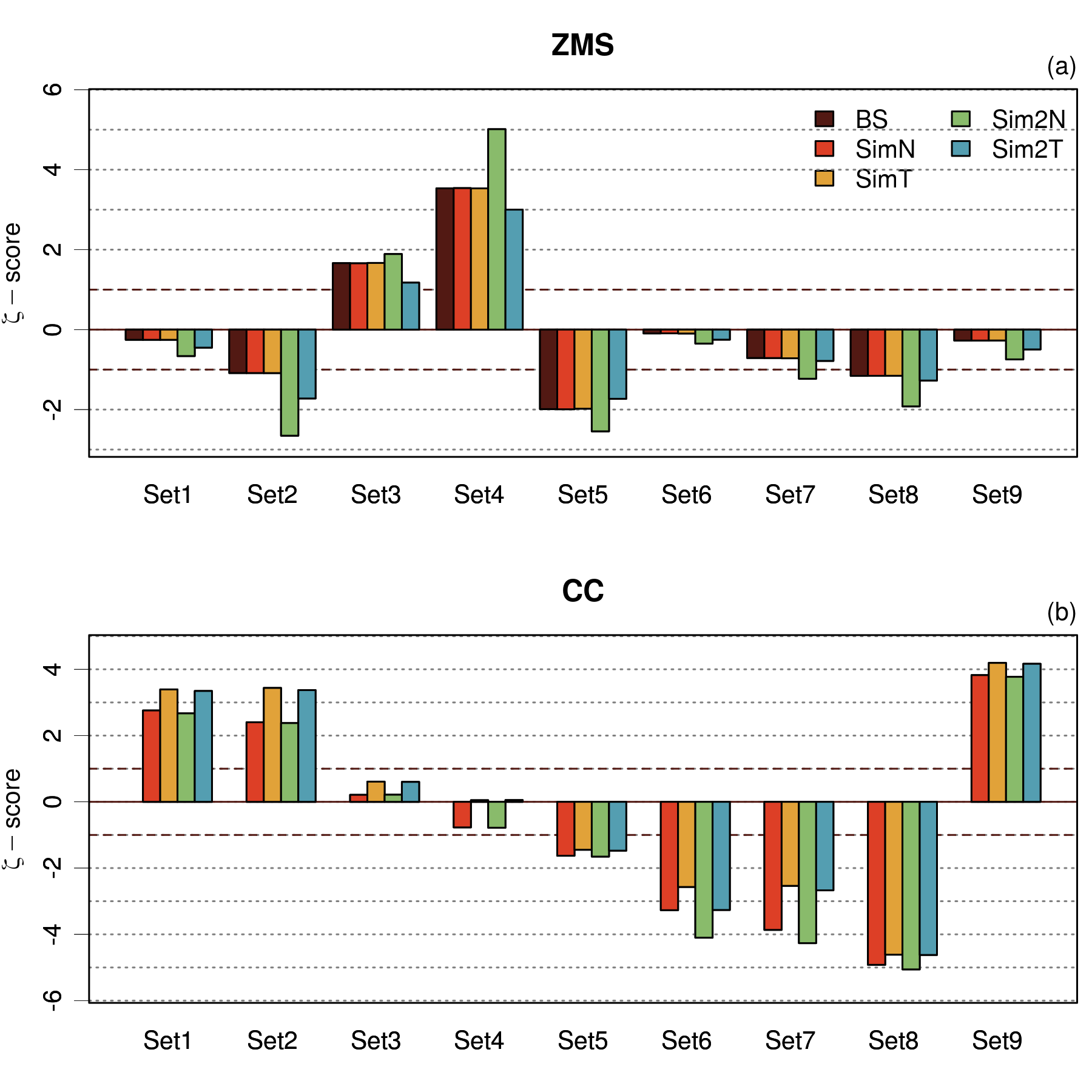
Let us first consider the results for the ZMS statistic [Figs. 8(a)]. There is a good agreement between the three bootstrapped CI-based estimations (BS, SimN, SimT). The absence of notable difference between the SimN and SimT results confirms the low sensitivity of this method to the choice of $D$. It is also clear that the Sim2N and Sim2T scores can differ notably from the other scores and between them, confirming a high sensitivity of the Monte Carlo CI $I_{D}$ to $D$. Sets 1-6 have been analyzed in an earlier study(Pernot2023d, ), by using the $\mathrm{Var}(Z)$ score and an approximate analytical estimation of confidence intervals(Cho2005, ). The validation results differ at the margin, as the approximate method used previously seems to provide slightly wider CIs than the bootstrapped ones used here, and is therefore less stringent.

For the CC statistic [Figs. 8(b)], it appears that the choice of $D$ has always a sizable effect, even for the Sim protocol. In consequence, and unless one trusts more one of the two options for $D$, the CC statistic cannot be reliably validated for the studied datasets. Note that, by chance and despite the amplitude of the $D$-induced discrepancies, all the CC validation statistics for a given dataset agree on the binary validation diagnostic. One might be then tempted to conclude that only Sets 3 and 4 have CCs compatible with their simulated reference values. Note that in this case, the Sim and Sim2 $\zeta$-scores for a given choice of $D$ are very similar.

Figure 9: Same as Fig. 8 for the ENCE and ZMSE consistency scores. In absence of a predefined reference value, the BS approach is not available for these statistics.

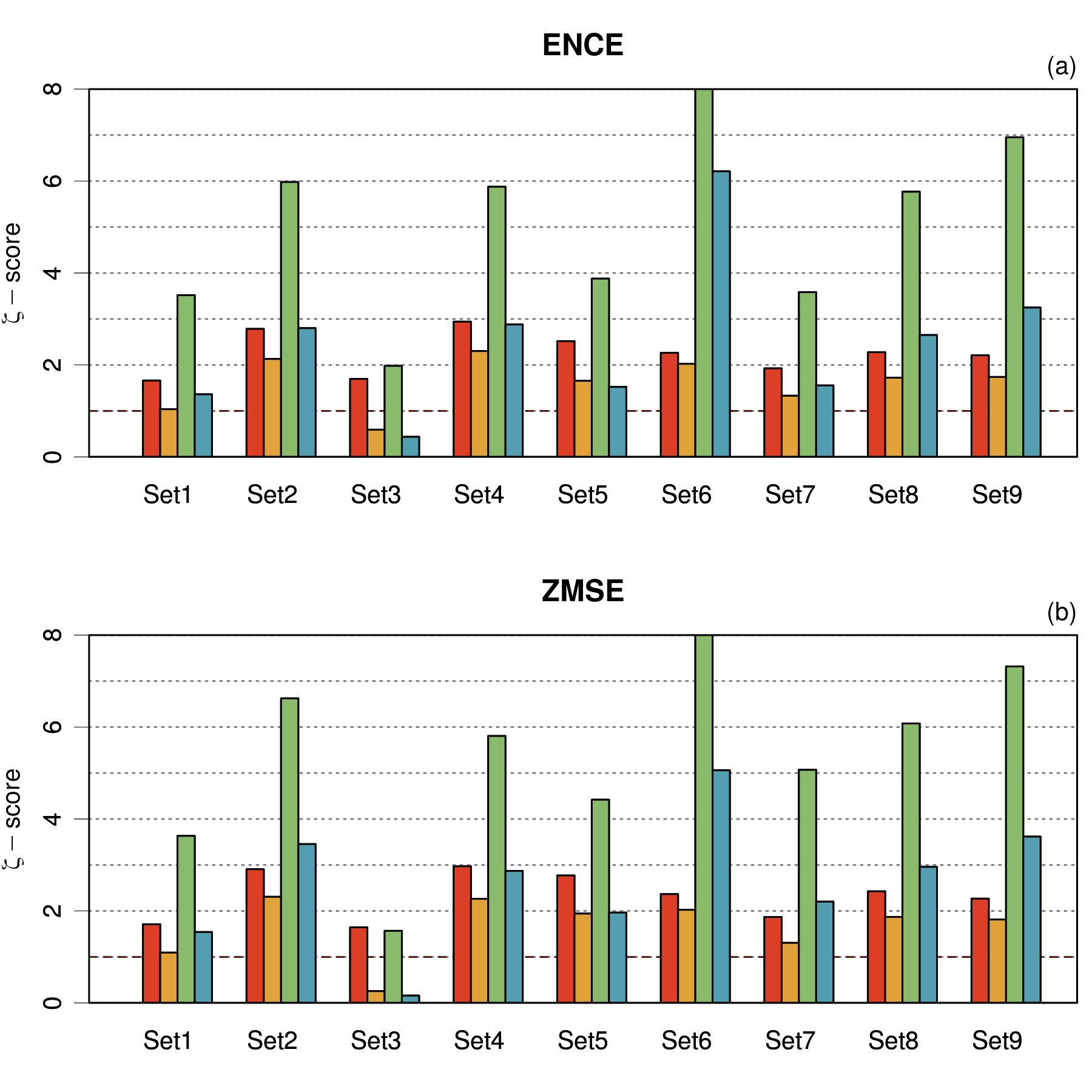
The $\zeta$-scores for the ENCE and ZMSE statistics have been estimated for $N=20$ bins and present very similar features (Fig.9): a notable sensitivity to $D$ and a large difference between the Sim and Sim2 protocols (except for Set 3). The latter observation confirms that one should not use the Monte Carlo CIs to estimate the $\zeta$-scores. Focusing one the SimN and SimT results, it appears that they globally agree to reject consistency, except for Set 3 where consistency would be validated by SimT, as observed in Appendix C.

IV Discussion

This study focuses on the validation of correlation and calibration statistics by standardized $\zeta$-scores, for which one needs reference values and confidence interval estimates. Reference values are predefined for the ZMS statistic, but not for CC, ENCE and ZMSE. In the latter cases, it is possible to generate reference values by a Monte Carlo approach, which implies to generate simulated error sets from the actual uncertainties, using a generative distribution $D$. A reference value and its standard error can be obtained by repeating this random sampling. The choice of an interval-based validation method results from the often marked non-normality of the error and uncertainty datasets, which prevents the use of more standard $z$-scores or $t$-scores. CIs are therefore estimated by bootstrapping for all statistics, by taking care that the bootstrap distributions can be non-normal and asymmetric.

In absence of a predefined reference, Pernot(Pernot2022c, ) and Rasmussen et al.(Rasmussen2023, ) proposed to use the standard deviation or CI of the simulated reference value as a metric to compare the estimated statistic to its reference value. This study shows unambiguously that several disadvantages come with this approach: (i) it introduces an asymmetry of treatment between the statistics with known and unknown reference values, using bootstrapping-based uncertainties for the former and simulation-based uncertainties for the latter(Rasmussen2023, ); (ii) the standard deviation (or CI) of the simulated reference values is strongly dependent on the chosen generative distribution $D$; and (iii) in such cases, validation becomes dependent on the often ad hoc choice of $D$.

To circumvent these issues, it is suggested here to use the bootstrapping-based intervals independently of the existence of a reference value, and to characterize the simulated reference by its standard error (standard deviation of the mean), which is much less sensitive to the choice of $D$. Moreover, with a moderate effort on the Monte Carlo sampling, it is possible to ensure that this standard error becomes negligible before the bootstrapping-based uncertainty, which solves the problem of the dependence of the $\zeta$-scores on the simulated reference uncertainty. The impact of this approach has been shown by comparing SimN to SimT and Sim2N to Sim2T (Figs.8-9): in all cases the proposed approach reduces the sensitivity to $D$, except for CC where it is about identical.

Another and less manageable source of sensitivity of the $\zeta$-scores to $D$ comes with the simulated reference value itself. For instance, the mean value of any statistic that involves a sign loss of the simulated errors (e.g. absolute value, squared value…) is likely to be affected by the shape/width of the errors distribution. This is particularly visible for the CC, ENCE and ZMSE statistics, but much less for the ZMS. For confidence curves, Pernot(Pernot2022c, ) has shown that the simulated reference based on the RMS of the errors was insensitive to $D$, which was not the case for the MAE. The sensitivity of a simulated reference value to the generative model has therefore to be directly assessed before using it for validation.

V Conclusion

This study sheds a critical look at the validation of an average calibration statistics (ZMS), a correlation statistic (CC) and two conditional calibration statistics (ENCE, ZMSE). A benchmark method was defined for those statistics with a predefined reference value (ZMS) and compared to simulation approaches for statistics with no predefined reference value (CC, ENCE and ZMSE). A validation workflow was proposed to deal with the main obstacles of the simulation approach (Fig. 1) and notably with the sensitivity of simulated reference values to the generative distribution $D$ used to generate ideal synthetic errors from actual uncertainties.

Important conclusions about the studied statistics have been obtained from a series of ML-UQ datasets from the literature.

• The generative distribution $D$ is not necessarily normal. The error distributions obtained by the generative model with a normal distribution $D$ (Eq. 1) rarely agree with the actual error distributions. Better fits are often obtained by using the distribution of scaled errors (z-scores) as a proxy. In some instances, e.g. Bayesian Neural Networks or Gaussian Processes, the generative distributions is prescribed, but this is not generally the case. Thus, before using an hypothetical generative distribution to simulate unknown reference values, one should test its pertinence for the dataset(s) under scrutiny.

• The use of simulated reference values for the CC, ENCE and ZMSE statistics is not reliable if $D$ is unknown. It has been shown that the simulated reference values for these statistics are highly sensitive to the choice of generative distribution $D$. If $D$ is unknown, one cannot estimate a reliable reference value for their validation. For CC, checking that it is positive is the best that can be done and there is not much sense in comparing CC values of different datasets (the largest value is not necessarily the better!). A much more powerful and reliable approach is the plotting of RMSE-based confidence curves with bootstrapped CI and simulated reference value. Similarly, the simulated reference values for measures such as the ENCE and ZMSE are very sensitive to the choice of $D$ and therefore cannot generally be used for validation of conditional calibration. When used for comparative studies, they should be limited to datasets of identical sizes and to identical binning schemes. Validation is possible by alternative approaches, such as the “extrapolation to zero bins” method used in Appendix C, or by the estimation of the “fraction of valid bins” proposed by Pernot(Pernot2023d, ). However, the reliability of the latter approach still needs to be demonstrated for a diversity of datasets.

Finally, the only case where the use of simulated reference values seems well adapted is for confidence curves, as the RMSE-based reference curve does not depend on $D$. However, there are probably other calibration statistics for which this concept might be useful, and the proposed workflow should enable to validate them with confidence.

Author Declarations

Conflict of Interest

The author has no conflicts to disclose.

Code and data availability

The code and data to reproduce the results of this article are available at https://github.com/ppernot/2024_SimRef/releases/tag/v1.0 and at Zenodo (https://doi.org/10.5281/zenodo.10730985).

Appendices

Appendix A Results tables for standardized scores

The numerical values necessary to build Fig. 8 are reported here (Tables A1-A4), with a summary of the necessary equations. Each table contains the values for one of the ZMS and CC statistics.

$\vartheta=ZMS$				BS								SimN, Sim2N									SimT, Sim2T
Set #	$\vartheta$			$\vartheta_{ref}$	$b_{BS}$		$I_{BS}$		$\zeta_{BS}$			$\tilde{\vartheta}_{ref}$		$u(\tilde{\vartheta}_{ref})$	$\zeta_{Sim}$		$I_{Sim2}$		$\zeta_{Sim2}$		$\tilde{\vartheta}_{ref}$		$u(\tilde{\vartheta}_{ref})$		$\zeta_{Sim}$		$I_{Sim2}$		$\zeta_{Sim2}$
1	0.	96		1	5.	3e-04	[0.	87, 1.12]	-0.	25		1.	00	3.1e-04	-0.	25	[0.	94, 1.06]	-0.66		1.	00	5.	0e-04	-0.	26	[0.	91, 1.10]	-0.45
2	0.	86		1	2.	6e-04	[0.	80, 0.99]	-1.	09		1.	00	2.3e-04	-1.	09	[0.	96, 1.04]	-2.65		1.	00	3.	7e-04	-1.	09	[0.	93, 1.07]	-1.72
3	1.	12		1	6.	5e-04	[1.	05, 1.20]	1.	66		1.	00	3.2e-04	1.	66	[0.	94, 1.06]	1.89		1.	00	4.	9e-04	1.	67	[0.	91, 1.10]	1.17
4	1.	23		1	-2.	6e-04	[1.	16, 1.30]	3.	53		1.	00	2.3e-04	3.	54	[0.	96, 1.04]	5.01		1.	00	3.	6e-04	3.	53	[0.	94, 1.08]	3.00
5	0.	85		1	5.	8e-04	[0.	78, 0.92]	-1.	99		1.	00	3.1e-04	-1.	99	[0.	94, 1.06]	-2.54		1.	00	4.	9e-04	-1.	98	[0.	91, 1.10]	-1.73
6	0.	98		1	-9.	1e-04	[0.	86, 1.15]	-0.	10		1.	00	2.3e-04	-0.	09	[0.	95, 1.04]	-0.35		1.	00	3.	6e-04	-0.	10	[0.	94, 1.07]	-0.25
7	0.	97		1	4.	9e-04	[0.	94, 1.01]	-0.	71		1.	00	1.2e-04	-0.	71	[0.	98, 1.02]	-1.23		1.	00	1.	9e-04	-0.	72	[0.	96, 1.04]	-0.78
8	0.	93		1	-2.	9e-04	[0.	87, 0.99]	-1.	16		1.	00	2.0e-04	-1.	16	[0.	96, 1.04]	-1.92		1.	00	3.	1e-04	-1.	15	[0.	94, 1.06]	-1.27
9	0.	97		1	1.	5e-03	[0.	90, 1.08]	-0.	27		1.	00	2.0e-04	-0.	27	[0.	96, 1.04]	-0.74		1.	00	3.	2e-04	-0.	27	[0.	94, 1.06]	-0.50

Table A1: Intermediate values for the estimation of $\zeta$-scores for the ZMS statistics.

$\vartheta=CC$				BS							SimN, Sim2N									SimT, Sim2T
Set #	$\vartheta$			$\vartheta_{ref}$	$b_{BS}$		$I_{BS}$		$\zeta_{BS}$		$\tilde{\vartheta}_{ref}$		$u(\tilde{\vartheta}_{ref})$	$\zeta_{Sim}$		$I_{Sim2}$		$\zeta_{Sim2}$		$\tilde{\vartheta}_{ref}$		$u(\tilde{\vartheta}_{ref})$		$\zeta_{Sim}$		$I_{Sim2}$	$\zeta_{Sim2}$
1	0.	50		n/a	-3.	1e-05	[0.	467, 0.536]	n/a		0.	40	1.9e-04	2.	76	[0.	38, 0.44]	2.67		0.	38	1.	9e-04	3.	39	[0.34, 0.42]	3.35
2	0.	62		n/a	-1.	2e-04	[0.	598, 0.641]	n/a		0.	57	1.1e-04	2.	40	[0.	55, 0.59]	2.38		0.	55	1.	1e-04	3.	44	[0.52, 0.57]	3.37
3	0.	26		n/a	-1.	8e-04	[0.	216, 0.300]	n/a		0.	25	2.1e-04	0.	21	[0.	21, 0.29]	0.21		0.	23	2.	1e-04	0.	61	[0.19, 0.27]	0.60
4	0.	40		n/a	6.	6e-05	[0.	372, 0.428]	n/a		0.	42	1.3e-04	-0.	77	[0.	40, 0.45]	-0.78		0.	40	1.	4e-04	0.	05	[0.37, 0.43]	0.05
5	0.	04		n/a	-1.	5e-04	[-0.	004, 0.081]	n/a		0.	11	2.2e-04	-1.	63	[0.	07, 0.15]	-1.65		0.	10	2.	2e-04	-1.	45	[0.06, 0.14]	-1.47
6	0.	40		n/a	-1.	4e-04	[0.	373, 0.433]	n/a		0.	50	1.2e-04	-3.	27	[0.	48, 0.52]	-4.10		0.	48	1.	2e-04	-2.	57	[0.46, 0.50]	-3.26
7	0.	31		n/a	7.	9e-06	[0.	297, 0.328]	n/a		0.	37	7.2e-05	-3.	86	[0.	36, 0.39]	-4.27		0.	35	7.	5e-05	-2.	54	[0.34, 0.37]	-2.67
8	-0.	03		n/a	-1.	2e-05	[-0.	052, 0.003]	n/a		0.	11	1.4e-04	-4.	92	[0.	08, 0.14]	-5.06		0.	10	1.	4e-04	-4.	61	[0.08, 0.13]	-4.62
9	0.	23		n/a	-1.	0e-04	[0.	207, 0.258]	n/a		0.	13	1.4e-04	3.	82	[0.	10, 0.16]	3.77		0.	12	1.	4e-04	4.	19	[0.09, 0.15]	4.17

Table A2: Same as Table A1 for the CC statistic.

$\vartheta=ENCE$				BS							SimN, Sim2N									SimT, Sim2T
Set #	$\vartheta$			$\vartheta_{ref}$	$b_{BS}$		$I_{BS}$		$\zeta_{BS}$		$\tilde{\vartheta}_{ref}$		$u(\tilde{\vartheta}_{ref})$	$\zeta_{Sim}$		$I_{Sim2}$		$\zeta_{Sim2}$		$\tilde{\vartheta}_{ref}$		$u(\tilde{\vartheta}_{ref})$		$\zeta_{Sim}$		$I_{Sim2}$	$\zeta_{Sim2}$
1	0.	125		n/a	0.	016	[0.	084, 0.153]	n/a		0.	056	9.5e-05	1.	66	[0.	038, 0.076]	3.52		0.	082	1.	5e-04	1.	04	[0.055, 0.114]	1.36
2	0.	126		n/a	0.	033	[0.	096, 0.130]	n/a		0.	041	7.0e-05	2.	78	[0.	028, 0.056]	5.98		0.	061	1.	1e-04	2.	13	[0.041, 0.085]	2.80
3	0.	097		n/a	0.	024	[0.	074, 0.101]	n/a		0.	058	9.8e-05	1.	70	[0.	040, 0.077]	1.98		0.	083	1.	5e-04	0.	59	[0.056, 0.115]	0.44
4	0.	135		n/a	0.	007	[0.	103, 0.157]	n/a		0.	043	7.4e-05	2.	94	[0.	029, 0.058]	5.88		0.	063	1.	2e-04	2.	30	[0.043, 0.088]	2.88
5	0.	131		n/a	0.	023	[0.	101, 0.139]	n/a		0.	056	9.4e-05	2.	52	[0.	039, 0.075]	3.88		0.	082	1.	5e-04	1.	66	[0.055, 0.114]	1.52
6	0.	244		n/a	0.	044	[0.	156, 0.276]	n/a		0.	045	8.1e-05	2.	26	[0.	030, 0.062]	11.7		0.	066	1.	3e-04	2.	02	[0.044, 0.095]	6.21
7	0.	066		n/a	0.	006	[0.	045, 0.085]	n/a		0.	026	5.3e-05	1.	93	[0.	017, 0.037]	3.58		0.	038	8.	3e-05	1.	33	[0.025, 0.056]	1.55
8	0.	108		n/a	0.	015	[0.	077, 0.118]	n/a		0.	036	6.0e-05	2.	28	[0.	025, 0.048]	5.77		0.	053	9.	7e-05	1.	72	[0.036, 0.074]	2.65
9	0.	120		n/a	0.	013	[0.	082, 0.140]	n/a		0.	036	6.0e-05	2.	21	[0.	025, 0.048]	6.95		0.	054	9.	7e-05	1.	74	[0.036, 0.074]	3.25

Table A3: Same as Table A1 for the ENCE statistic.

$\vartheta=ZMSE$				BS							SimN, Sim2N									SimT, Sim2T
Set #	$\vartheta$			$\vartheta_{ref}$	$b_{BS}$		$I_{BS}$		$\zeta_{BS}$		$\tilde{\vartheta}_{ref}$		$u(\tilde{\vartheta}_{ref})$	$\zeta_{Sim}$		$I_{Sim2}$		$\zeta_{Sim2}$		$\tilde{\vartheta}_{ref}$		$u(\tilde{\vartheta}_{ref})$		$\zeta_{Sim}$		$I_{Sim2}$	$\zeta_{Sim2}$
1	0.	255		n/a	0.	034	[0.	172, 0.299]	n/a		0.	112	1.9e-04	1.	71	[0.	077, 0.152]	3.63		0.	164	2.	9e-04	1.	09	[0.111, 0.223]	1.54
2	0.	273		n/a	0.	072	[0.	207, 0.283]	n/a		0.	082	1.4e-04	2.	91	[0.	056, 0.111]	6.62		0.	121	2.	1e-04	2.	31	[0.083, 0.165]	3.46
3	0.	173		n/a	0.	048	[0.	136, 0.180]	n/a		0.	112	1.9e-04	1.	64	[0.	077, 0.151]	1.57		0.	163	2.	8e-04	0.	26	[0.110, 0.223]	0.16
4	0.	247		n/a	0.	011	[0.	191, 0.287]	n/a		0.	082	1.4e-04	2.	97	[0.	056, 0.110]	5.81		0.	121	2.	1e-04	2.	26	[0.083, 0.165]	2.87
5	0.	283		n/a	0.	052	[0.	221, 0.304]	n/a		0.	112	1.9e-04	2.	77	[0.	077, 0.151]	4.42		0.	163	2.	9e-04	1.	94	[0.111, 0.224]	1.96
6	0.	356		n/a	0.	270	[0.	240, 0.357]	n/a		0.	082	1.4e-04	2.	37	[0.	056, 0.111]	9.53		0.	121	2.	2e-04	2.	02	[0.082, 0.168]	5.06
7	0.	118		n/a	0.	018	[0.	078, 0.131]	n/a		0.	043	7.2e-05	1.	87	[0.	029, 0.058]	5.07		0.	066	1.	2e-04	1.	31	[0.045, 0.089]	2.20
8	0.	225		n/a	0.	033	[0.	162, 0.246]	n/a		0.	071	1.2e-04	2.	43	[0.	049, 0.097]	6.08		0.	107	1.	9e-04	1.	87	[0.072, 0.147]	2.96
9	0.	250		n/a	0.	025	[0.	171, 0.287]	n/a		0.	071	1.2e-04	2.	27	[0.	049, 0.096]	7.32		0.	107	1.	9e-04	1.	81	[0.073, 0.147]	3.62

Table A4: Same as Table A1 for the ZMSE statistic.

All standardized $\zeta$-scores are built from the equation

$$\zeta(\vartheta_{est},\vartheta_{ref},I)=\begin{cases}\frac{\vartheta_{est}-\vartheta_{ref}}{I^{+}-\vartheta_{est}}&if\,(\vartheta_{est}-\vartheta_{ref})\leq 0\\ \frac{\vartheta_{est}-\vartheta_{ref}}{\vartheta_{est}-I^{-}}&if\,(\vartheta_{est}-\vartheta_{ref})>0\end{cases}$$ (26)

where $\vartheta_{est}$ is the estimated value of the statistic, $\vartheta_{ref}$ is its reference value, and $I=[I^{-},I^{+}]$ is a 95% confidence interval. The values of $\vartheta_{ref}$ and $I$ are estimated according to three schemes

Scheme	$\vartheta_{ref}$	$I$
BS	Predefined	Bootstrapped
Sim	Monte Carlo	Bootstrapped
Sim2	Monte Carlo	Monte Carlo

In the absence of a predefined reference value, $\zeta_{BS}$ cannot be estimated.

In the Sim and Sim2 schemes, synthetic error sets are generated according to

$$E_{i}=u_{E,i}\epsilon_{i}$$ (27)

where $u_{E,i}$ is one of the uncertainties in the original dataset, and $\epsilon_{i}$ is a random value from the generative distribution $D$ ($\epsilon_{i}\sim D(0,1)$ ). Two variants of $D$ are considered in the present study, denoted N and T:

N

a standard normal distribution $D=N(0,1)$

T

a unit_variance Student’s-t distribution $D=t_{s}(6)$

One has thus five options for the estimation of standardized scores: $\zeta_{BS}$, $\zeta_{SimN}$, $\zeta_{Sim2N}$, $\zeta_{SimT}$, $\zeta_{Sim2T}$, which are reported in the results tables with intermediate results and in Fig. 8.

Appendix B Reference values for the ENCE and ZMSE statistic

The ENCE and ZMSE statistics have been shown previously to depend on the binning scheme(Pernot2023a_arXiv, ). We consider here other sources of influence, such as the dataset size, and uncertainty distribution shape. This study is performed on synthetic datasets, and the dependence on the generative model is also assessed.

Simulated reference values $\tilde{\vartheta}_{D,ref}$ for the ENCE and ZMSE statistics have been estimated from $N_{MC}=5000$ synthetic calibrated datasets generated by the NIG model

$$E \sim u_{E}\times N(0,1)$$ (28)

$$u_{E}^{2} \sim IG(\nu/2,\nu/2)$$ (29)

with three varying parameters: the dataset size $M\in\left\{2000,4000,8000,12000,16000\right\}$ , the number of equal-size bins $N\in\left\{10,20,30,40,50\right\}$ and the shape of the uncertainty distribution $\nu\in\left\{3,4,5,6,12,24\right\}$. The relative uncertainties on the reported mean reference values are around $1.5\thinspace 10^{-3}$. The results are shown in Fig. A1.

Figure A1: Sensitivity of simulated ENCE and ZMSE values to the dataset size ($M$), number of bins ($N$) and shape of the uncertainty distribution ($\nu$), for calibrated datasets generated from the NIG model.

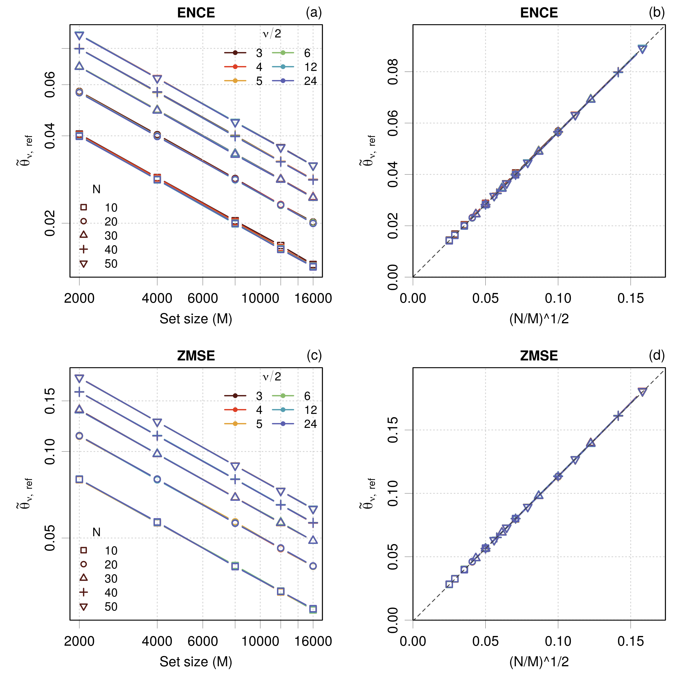
The dependence of the ENCE on the number of bins was shown in a previous study(Pernot2023a_arXiv, ) to be in $N^{1/2}$. The log-log plot in Fig. A1(left) reveals that the ENCE depends also on $M$ as a power law. One has thus $ENCE=\alpha M^{\beta}N^{1/2}$ with $\beta\simeq-1/2$. The same data are then plot on a linear scale as a function of $(N/M)^{1/2}$, from which one can see a perfect linear fit by $\tilde{\vartheta}_{N,ref}=\alpha\times(N/M)^{1/2}$ with $\alpha\simeq 0.56$. The ZMSE presents features very similar to the ENCE, with a different slope, $\tilde{\vartheta}_{N,ref}\simeq 1.14\times(N/M)^{1/2}$. In both cases, the impact of the uncertainty distribution is minor, albeit larger for ENCE than for ZMSE, and negligible for the validation process.

It seems therefore that, for a normal generative model and a chosen binning scheme, it is possible to define a reference value for the ENCE and ZMSE statistics for each dataset. The availability of a predefined reference value would considerably simplify the validation approach, when compared to the extrapolation-based one proposed by Pernot(Pernot2023a_arXiv, ).

Let us now check the sensitivity of this approach to the generative distribution. The same protocol as above is followed for another choice of generative model (denoted T6IG)

$$E \sim u_{E}\times t_{s}(6)$$ (30)

$$u_{E}^{2} \sim IG(\nu/2,\nu/2)$$ (31)

and the results are shown in Fig. A2.

Figure A2: Same as Fig. A1 for the T6IG model.

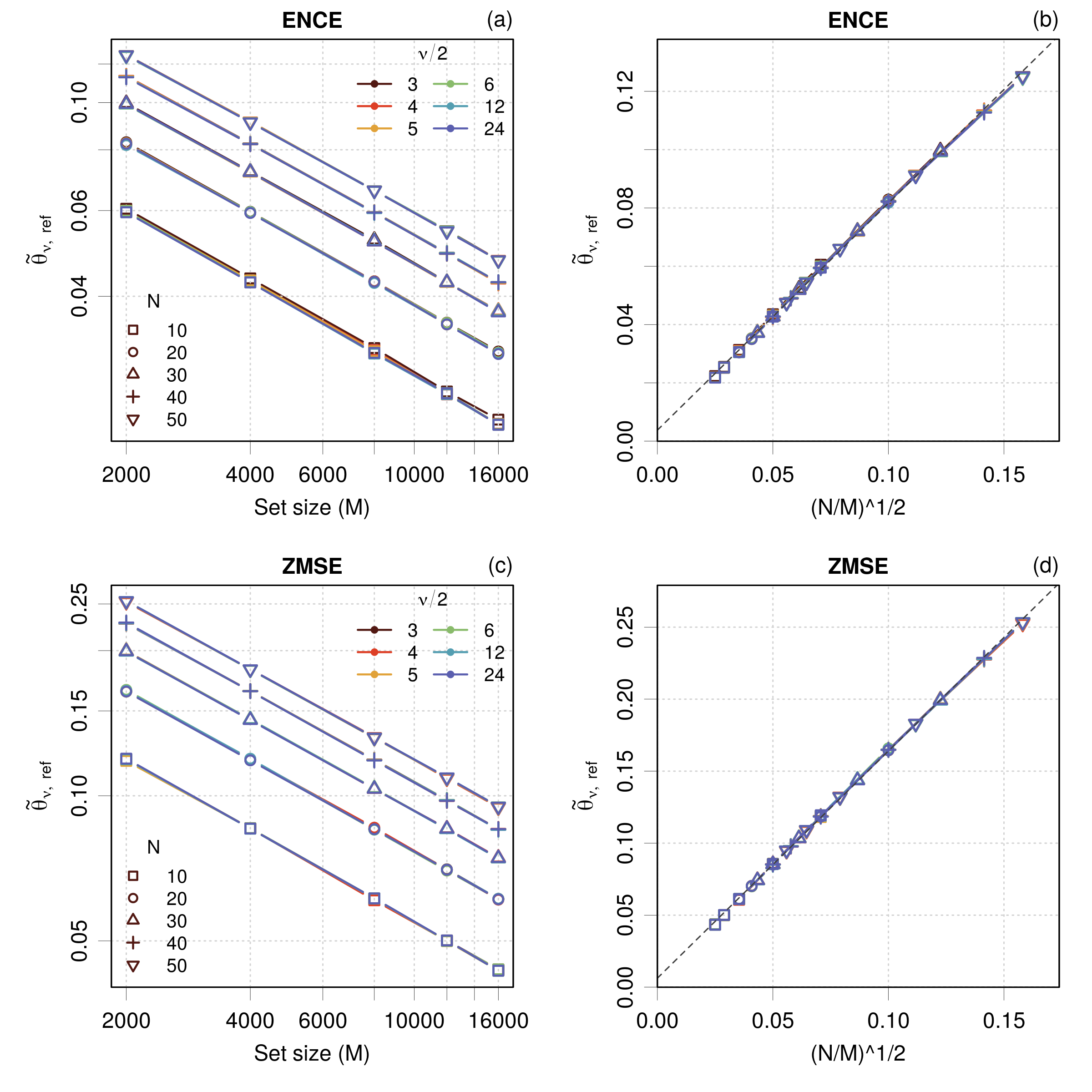
The same linear relationship as for the normal generative distribution is observed, but, in each case, with a different slope and a small positive intercept. Besides, a very small deviation from linearity can also be perceived. For ENCE, one gets then $\tilde{\vartheta}_{T,ref}\simeq 0.004+0.779\times(N/M)^{1/2}$ and for ZMSE $\tilde{\vartheta}_{T,ref}\simeq 0.006+1.577\times(N/M)^{1/2}$.

It seems thus impossible to define a reference value for ENCE and ZMSE if the generative distribution is unknown.

Appendix C Validation of ZMSE for the application datasets

For each of the nine datasets, one establishes a ZMSE validation diagnostic by a method which is independent of a generative distribution hypothesis. For this, the ZMSE is estimated for a series of bin numbers $N$ between 10 and 150, with the constraint that bins should not contain less than 20 data points. The data with $N>20$ are fitted by a linear model as a function of $(N/M)^{1/2}$. The intercept of the regression line is then compared to zero.(Pernot2023a_arXiv, ) The reference lines for the NIG and T6IG models defined in Appendix B are also plotted for comparison.

Figure A3: Validation of ZMSE by the extrapolation method: ZMSE are estimated for a sequence of bin numbers and plotted as function of $(N/M)^{1/2}$ (blue dots); this sequence (for $N>20$) is fitted by a linear model (solid red line); reference lines are plotted for the NIG (dashed line) and T6IG (dotted line) models.

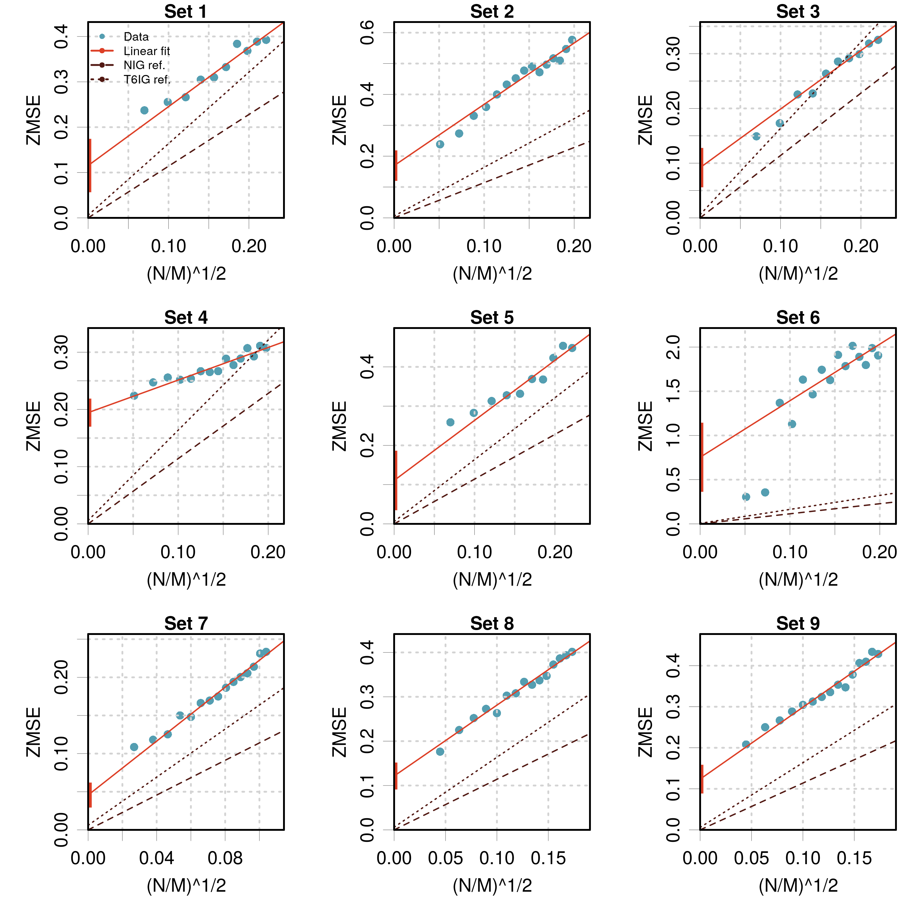
All the datasets are failing this validation test of conditional calibration (consistency), as none of the red intervals encloses the origin. Note however that for some datasets (e.g. Sets 3 and 4), it is possible to choose a number of bins such that the ZMSE is compatible with the T6IG reference (dotted line). This shows the danger of using a reference value from an unconstrained generative model.

References

- (1) M. Tynes, W. Gao, D. J. Burrill, E. R. Batista, D. Perez, P. Yang, and N. Lubbers. Pairwise difference regression: A machine learning meta-algorithm for improved prediction and uncertainty quantification in chemical search. J. Chem. Inf. Model., 61:3846–3857, 2021. PMID: 34347460.
- (2) P. Pernot. Prediction uncertainty validation for computational chemists. J. Chem. Phys., 157:144103, 2022.
- (3) D. Levi, L. Gispan, N. Giladi, and E. Fetaya. Evaluating and Calibrating Uncertainty Prediction in Regression Tasks. Sensors, 22:5540, 2022.
- (4) P. Pernot. Properties of the ENCE and other MAD-based calibration metrics. arXiv:2305.11905, May 2023.
- (5) P. Pernot. Confidence curves for UQ validation: probabilistic reference vs. oracle. arXiv:2206.15272, June 2022.
- (6) M. H. Rasmussen, C. Duan, H. J. Kulik, and J. H. Jensen. Uncertain of uncertainties? A comparison of uncertainty quantification metrics for chemical data sets. J. Cheminf., 15:1–17, December 2023.
- (7) K. Tran, W. Neiswanger, J. Yoon, Q. Zhang, E. Xing, and Z. W. Ulissi. Methods for comparing uncertainty quantifications for material property predictions. Mach. Learn.: Sci. Technol., 1:025006, 2020.
- (8) BIPM, IEC, IFCC, ILAC, ISO, IUPAC, IUPAP, and OIML. Evaluation of measurement data - Guide to the expression of uncertainty in measurement (GUM). Technical Report 100:2008, Joint Committee for Guides in Metrology, JCGM, 2008. URL: http://www.bipm.org/utils/common/documents/jcgm/JCGM_100_2008_F.pdf.
- (9) J. Busk, P. B. Jørgensen, A. Bhowmik, M. N. Schmidt, O. Winther, and T. Vegge. Calibrated uncertainty for molecular property prediction using ensembles of message passing neural networks. Mach. Learn.: Sci. Technol., 3:015012, 2022.
- (10) A. Amini, W. Schwarting, A. Soleimany, and D. Rus. Deep Evidential Regression. arXiv:1910.02600, October 2019.
- (11) M. Evans, N. Hastings, and B. Peacock. Statistical Distributions. Wiley-Interscience, 3rd edition, 2000.
- (12) P. Pernot. How to validate average calibration for machine learning regression tasks ? arXiv:2402.10043, February 2024. URL: https://arxiv.org/abs/2402.10043.
- (13) P. Pernot. Calibration in machine learning uncertainty quantification: Beyond consistency to target adaptivity. APL Mach. Learn., 1:046121, 2023.
- (14) P. Pernot. The long road to calibrated prediction uncertainty in computational chemistry. J. Chem. Phys., 156:114109, 2022.
- (15) J. Busk, M. N. Schmidt, O. Winther, T. Vegge, and P. B. Jørgensen. Graph neural network interatomic potential ensembles with calibrated aleatoric and epistemic uncertainty on energy and forces. Phys. Chem. Chem. Phys., 25:25828–25837, 2023.
- (16) W. Zhang, Z. Ma, S. Das, T.-W. Weng, A. Megretski, L. Daniel, and L. M. Nguyen. One step closer to unbiased aleatoric uncertainty estimation. arXiv:2312.10469, December 2023.
- (17) T. Gneiting, F. Balabdaoui, and A. E. Raftery. Probabilistic forecasts, calibration and sharpness. J. R. Statist. Soc. B, 69:243–268, 2007.
- (18) P. Pernot. Can bin-wise scaling improve consistency and adaptivity of prediction uncertainty for machine learning regression ? arXiv:2310.11978, October 2023.
- (19) T. J. DiCiccio and B. Efron. Bootstrap confidence intervals. Statist. Sci., 11:189–212, 1996. URL: https://www.jstor.org/stable/2246110.
- (20) G. Palmer, S. Du, A. Politowicz, J. P. Emory, X. Yang, A. Gautam, G. Gupta, Z. Li, R. Jacobs, and D. Morgan. Calibration after bootstrap for accurate uncertainty quantification in regression models. npj Comput. Mater., 8:115, 2022.
- (21) R. A. Groeneveld and G. Meeden. Measuring skewness and kurtosis. The Statistician, 33:391–399, 1984. URL: http://www.jstor.org/stable/2987742.
- (22) P. Pernot and A. Savin. Using the Gini coefficient to characterize the shape of computational chemistry error distributions. Theor. Chem. Acc., 140:24, 2021.
- (23) P. Pernot, B. Huang, and A. Savin. Impact of non-normal error distributions on the benchmarking and ranking of Quantum Machine Learning models. Mach. Learn.: Sci. Technol., 1:035011, 2020.
- (24) E. Cho, M. J. Cho, and J. Eltinge. The variance of sample variance from a finite population. Int. J. Pure Appl. Math., 21:387–394, 2005. URL: http://www.ijpam.eu/contents/2005-21-3/10/10.pdf.