Enhancing Biomechanical Simulations Based on A Posteriori Error Estimates: The Potential of Dual Weighted Residual-Driven Adaptive Mesh Refinement

Abstract

The Finite Element Method (FEM) is a well-established procedure for computing approximate solutions to deterministic engineering problems described by partial differential equations. FEM produces discrete approximations of the solution with a discretisation error that can be an be quantified with a posteriori error estimates. The practical relevance of error estimates for biomechanics problems, especially for soft tissue where the response is governed by large strains, is rarely addressed. In this contribution, we propose an implementation of a posteriori error estimates targeting a user-defined quantity of interest, using the Dual Weighted Residual (DWR) technique tailored to biomechanics. The proposed method considers a general setting that encompasses three-dimensional geometries and model non-linearities, which appear in hyperelastic soft tissues. We take advantage of the automatic differentiation capabilities embedded in modern finite element software, which allows the error estimates to be computed generically for a large class of models and constitutive laws. First we validate our methodology using experimental measurements from silicone samples, and then illustrate its applicability for patient-specific computations of pressure ulcers on a human heel.

1 Introduction

The importance of finite element analyses (FEA) for biomechanical investigations has increased considerably worldwide in recent years. Such finite element models are widely employed to investigate both the underlying mechanisms that drive normal physiology of biological soft tissues and the mechanical factors that contribute to the onset and development of diseases such as tumour growth [61, 55]), atherosclerosis or aneurysms [49], or multilevel lumbar disc degenerative diseases [50], to name a few. Finite element models are also valuable tools that contribute to the development of medical devices such as, for example, vascular stent-grafts [45], and have the potential to improve prevention strategies [28, 54, 32], surgical planning [57, 51, 8], pedagogical simulators for medical training [29, 14] and guidance of surgeons during interventions [59, 12]. A survey of applications using simulation modelling for healthcare sector can be found for instance in [37].

In this context, one major issue is meshing, since the reliability of the predicted mechanical response arising from computer simulation heavily relies on the quality of the underlying finite element mesh [23]. The patient-specific mesh has to be built from segmented medical images (CT, MRI, ultra-sound), and has to conform to anatomical details with potentially complex topologies and geometries [6]. In general the quality of a given mesh is assessed through purely geometrical criteria, that allow in some way to quantify the distortion of the geometry of the elements [9]. Beyond mesh quality, mesh density is another, related, parameter which must be controlled during biomechanics simulations. Moreover solutions must be obtained on commodity hardware within clinical time scales: milliseconds (for surgical training); minutes (for surgical assistance); hours (for surgical planning). As a result one question that always arises in practice is: “Given a tolerable error level, what is the coarsest possible mesh which will provide the required accuracy?” This leads to the notion of “mesh optimality”, which is achieved for an optimal balance between the accuracy in a given quantity of interest to the user and the associated computational cost.

In this paper, we investigate the capability of a posteriori error estimates [1, 58] to provide useful information about the discretization error, i.e., the difference between the finite element solution and the exact solution of the same boundary value problem on the same geometry. A posteriori error estimates are quantities computed from the numerical solution, that indicate the magnitude of the local error. These estimates are at the core of mesh adaptive techniques [39]. Many a posteriori error estimation methods have been developed in the numerical analysis community. These methods have different theoretical and practical properties. However, despite their great potential, error estimates have rarely been considered for patient-specific finite element simulations in the biomechanical community.

To the best of our knowledge, the first works that address this issue are [11, 10], which study the discretization error (based on energy norm) of real-time simulations using the recovery-based technique of Zienkiewicz and Zhu [62]. This approach is inexpensive and allows to deal with real-time simulations. However, the error in energy norm might not provide useful information for applications where one is interested in the error of a real physical quantity of interest. To overcome this difficulty, estimates based on duality arguments are common for a posteriori error estimation, see e.g. [3, 26, 41, 46, 34, 20]. A preliminary study has been carried out previously in this direction in [16] by the authors of the present paper. This study makes use of the Dual Weighted Residuals (DWR) method, as presented in [3]. Let us recall that the main idea of this method is to solve a dual problem, the solution of which is used as a weight that indicates locally the sensitivity of the quantity of interest for each cell-wise contribution to the discretization error. However, this aforementioned study is limited to a simplified setting, since it was aimed at giving preliminary insights and at addressing the first technical difficulties. The modelling of soft tissues in [16] is indeed restricted to two-dimensional linear elasticity (plane strain) problems and to a quantity of interest that should depend linearly of the displacement.

As a result, the main goal of this paper is to handle a setting much closer to current practice in soft tissue simulation. For this purpose, we consider three-dimensional (passive) hyperelastic soft tissue and arbitrary quantities of interest, that may depend non-linearly on the displacement. The DWR method is very well adapted to this setting, as it was designed originally for non-linear problems [3] (see also [30, 60, 21, 22] for applications in non-linear elasticity). Nevertheless, one major issue for its application is the practical calculation of the dual solution, which involves the derivatives of the primal weak form and of the quantity of interest (this problem does not appear in the linear setting). This formal derivation can be intricate for soft tissue models built from complex hyperelastic constitutive laws. To handle this issue, we take advantage of the capabilities of modern finite element softwares such as FEniCS or GetFEM++, that integrate automatic symbolic differentiation. Not only it makes easier the implementation of the DWR method for error estimation, but also it requires no real effort if the constitutive law is changed. Then, we validate the methodology using experimental data obtained from in-vitro study of silicone samples [36] and show its potential interest on an example coming from patient-specific simulation.

This paper is organized as follows. In Section 2, we describe the hyperelastic setting for passive soft tissue, the corresponding finite element discretization, the DWR a posteriori error estimation as well as the algorithm for mesh refinement. In Section 3, we illustrate the methodology for different test-cases. The results are discussed in Section 4.

2 Methods

First we present the model problem, then the finite element discretization and finally the error estimation and mesh refinement techniques.

2.1 Problem setting: incompressible hyperelastic soft tissue

We consider an (incompressible) hyperelastic body in a reference configuration denoted by $\Omega$, an open subset of $\mathbb{R}^{3}$, and subjected to a given body force $\bm{B}$. The unknown displacement field and the unknown static pressure are denoted by $\bm{u}$ and $\bm{p}$, respectively. The deformation gradient is denoted $\bm{F}$, with $\bm{F}:=\bm{I}+\nabla_{X}\bm{u}$, where $\bm{I}$ stands for the identity matrix, and $\nabla_{X}$ denotes the gradient with respect to coordinates in the reference configuration. The first Piola-Kirchhoff stress tensor denoted $\bm{\Pi}$ is derived from the hyperelastic strain-energy density function $W$, which depends on the displacement field $\bm{u}$ and the pressure $\bm{p}$, as follows:

$$\bm{\Pi}=\frac{\partial W}{\partial\bm{F}}.$$ (1)

In the present paper, we will consider different incompressible material models corresponding to some strain-energy densities, namely:

1. Mooney-Rivlin model (see [38]):

   $$W:=c_{10}(J_{1}-3)+c_{01}(J_{2}-3)-\bm{p}(\mbox{det}(\bm{C})-1)$$ (2)

2. Gent model (see [19]) :

   $$W:=\frac{-EJ_{m}}{6}\ln\left(1-\frac{J_{1}-3}{J_{m}}\right)-\bm{p}(\mbox{det}(\bm{C})-1)$$ (3)

3. Haines-Wilson model (see [27]):

   $$W:=c_{10}(J_{1}-3)+c_{01}(J_{2}-3)+c_{20}(J_{1}-3)^{2}+c_{02}(J_{2}-3)^{2}\\ +c_{30}(J_{1}-3)^{3}+c_{11}(J_{1}-3)(J_{2}-3)-\bm{p}(\mbox{det}(\bm{C})-1)$$ (4)

where $\bm{C}(:=\bm{F}^{T}\cdot\bm{F})$ denote the right Cauchy-Green tensor, $J:=\textrm{det }\bm{F}$ the jacobian of the deformation, where $I_{1}:=\textrm{trace }\bm{C}$, $I_{2}:=\frac{1}{2}((\textrm{tr }\bm{C})^{2}-\textrm{tr }(\bm{C}\cdot\bm{C}))$, $J_{1}:=I_{1}J^{-\frac{2}{3}}$ and $J_{2}:=I_{2}J^{-\frac{4}{3}}$ are invariants associated to the deformation and $c_{ij}$, $J_{m}$ and $E$ are some coefficients which will be given in Table 1. For the sake of simplicity, the boundary $\partial\Omega$ of $\Omega$ is partitioned into two subsets $\Gamma_{D}$ and $\Gamma_{N}$, and we apply a prescribed displacement $\bm{u}=\bm{u}_{D}$ on $\Gamma_{D}$ and a given force $\bm{T}$ on $\Gamma_{N}$.

Let us introduce the virtual works associated to the internal and external forces:

$$A(\bm{u},\bm{p};\bm{v},\bm{q}):=\int_{\Omega}\bm{\Pi}(\bm{u},\bm{p}):\nabla_{X}\bm{v}\,\mathrm{d}\Omega+\int_{\Omega}(1-\mathrm{det}(\bm{C}))\bm{q}\,\mathrm{d}\Omega,\qquad L(\bm{v}):=\int_{\Omega}\bm{B}\cdot\bm{v}\,\mathrm{d}\Omega+\int_{\Gamma_{N}}\bm{T}\cdot\bm{v}\,\mathrm{d}\Gamma,$$

where $\bm{u}$ and $\bm{v}$ are admissible displacements and $\bm{p}$ and $\bm{q}$ are admissible pressures. The hyperelastic problem in weak form reads

$$\left\{\begin{array}[]{l}\text{Find a displacement }\bm{u},\text{with }\bm{u}=\bm{u}_{D}\text{ on }\Gamma_{D}\text{ and a pressure }\bm{p}\text{ such that }\\ \vskip 3.0pt plus 1.0pt minus 1.0pt\cr A(\bm{u},\bm{p};\bm{v},\bm{q})=L(\bm{v}),\,\forall(\bm{v},\bm{q}),\,\bm{v}=\mathbf{0}\text{ on }\Gamma_{D},\end{array}\right.$$ (5)

Let $\mathcal{K}_{h}$ be a mesh of the domain $\Omega$. Let us denote by $\bm{V}_{h}\times\bm{Q}_{h}$ the finite element pair that makes use of the lowest-order Taylor-Hood finite elements on $\mathcal{K}_{h}$ (continuous piecewise polynomials of order $2$ for the displacement and of order $1$ for the pressure). The finite element method to solve our hyperelastic problem reads

$$\left\{\begin{array}[]{l}\text{Find a displacement }\bm{u}_{h}\in\bm{V}_{h}\text{, with }\bm{u}_{h}=\bm{u}_{D}^{h}\text{ on }\Gamma_{D}\text{ and a pressure }\bm{p}_{h}\in\bm{Q}_{h}\text{ such that }\\ \vskip 3.0pt plus 1.0pt minus 1.0pt\cr A(\bm{u}_{h},\bm{p}_{h};\bm{v}_{h},\bm{q}_{h})=L(\bm{v}_{h}),\,\forall(\bm{v}_{h},\bm{q}_{h})\in\bm{V}_{h}^{0}\times\bm{Q}_{h},\end{array}\right.$$ (6)

where $\bm{V}_{h}^{0}$ is composed by the functions of $\bm{V}_{h}$ vanishynig on $\Gamma_{D}$ and where $u_{D}^{h}$ is a finite element approximation of $u_{D}$, obtained for instance by Lagrange interpolation or by projection.

Note that the above choice of Taylor-Hood finite elements is for the sake of simplicity, and that the methodology described below for mesh refinement can be extended rather straightforwardly to other conforming variational discretization techniques, provided they ensure a stable and accurate approximation of the finite elasticity equations, and that they allow to split the residual as a sum of local contributions. For instance, any other infsup stable pair of finite elements (mini-element, P2-iso-P1) on simplicial, tensor-product or mixed meshes can be considered.

2.2 Quantity of interest

The objective of goal-oriented error estimation is to estimate the error of the finite element solution for a user-defined quantity, possibly different from the energy norm, see [2, 3, 20, 21, 40]. The idea of this technique comes from the fact that one would like to analyse the error of a predefined target quantity since in certain circumstances the global error norm may not be useful.

Let $Q(\bm{u},\bm{p})$ be a quantity of biomechanical interest computed from the exact solution $(\bm{u},\bm{p})$ of the problem (5), with smooth, but possibly nonlinear, dependence on $(\bm{u},\bm{p})$. The aim is to estimate the error for the quantity of interest

$$|Q(\bm{u},\bm{p})-Q(\bm{u}_{h},\bm{p}_{h})|$$

where $(\bm{u}_{h},\bm{p}_{h})$ is the approximated finite element solution of (6).

2.3 Dual problem for computing the weights

One of the main ingredients of the DWR method is to solve an adjoint problem to extract information from the quantity of interest, and get feedback about the regions where it is more, or less, influenced, by the approximation error. As a result, we compute a pair of dual variables $(\bm{z}_{h},\bm{w}_{h})$ by solving

$$\left\{\begin{array}[]{l}\text{Find }({\bm{z}}_{h},\bm{w}_{h})\in{\bm{V}}_{h}^{0}\times\bm{Q}_{h}\text{ such that }\\ \vskip 3.0pt plus 1.0pt minus 1.0pt\cr(A^{\prime})^{*}(\bm{u}_{h},\bm{p}_{h}|{\bm{z}}_{h},{\bm{w}}_{h};{\bm{v}}_{h},{\bm{q}}_{h})=Q^{\prime}(\bm{u}_{h},\bm{p}_{h}|{\bm{v}}_{h},\bm{q}_{h})\quad\forall({\bm{v}}_{h},\bm{q}_{h})\in{\bm{V}}_{h}^{0}\times\bm{Q}_{h},\end{array}\right.$$ (7)

where $A^{\prime}$ and $Q^{\prime}$ denote the Fréchet derivative of $A$ and $Q$, respectively, and $(A^{\prime})^{*}$ is the adjoint form of $A^{\prime}$. Then we extrapolate the solution in a finite element space of higher polynomial degree following [48, Fig. 5.1]. This function weights the residual in our estimator.

Remark that the dual problem (7) is linear, so solving it is not expensive in comparison to (5). For model problems such as (5), and some expressions of $Q$, the practical calculation of $A^{\prime}$ and $Q^{\prime}$ can be tough. For this purpose, we take advantage of the capabilities of automatic symbolic differentiation embedded into modern finite element software such as FEniCS or GetFEM++. Furthermore, this feature makes possible some genericity in the implementation: virtually nothing has to be changed in the program if the hyperelastic constitutive law is modified.

2.4 The representation formula of Becker and Rannacher

We introduce $r(\bm{u}_{h},\bm{p}_{h};\bm{v},\bm{q})$ the residual of Problem (6) as

$$r(\bm{u}_{h},\bm{p}_{h};\bm{v},\bm{q})=L(\bm{v},\bm{q})-A(\bm{u}_{h},\bm{p}_{h};\bm{v},\bm{q})\qquad\forall(\bm{v},\bm{q})\in\bm{V}\times\bm{Q}.$$ (8)

This, roughly speaking, quantifies how well the hyperelasticity equations are approximated (it should tendsto zero if the mesh is uniformly refined). Thanks to the dual system (7), we obtain expression of the error on $Q$ as a best approximation term involving the residual and the (exact) dual solution (see [3, Proposition 2.3]):

$$Q(\bm{u},\bm{p})-Q(\bm{u}_{h},\bm{p}_{h})=\min_{(\bm{v}_{h},\bm{q}_{h})\in\bm{V}_{h}\times\bm{Q}_{h}}r(\bm{u}_{h},\bm{p}_{h};\bm{z}-\bm{v}_{h},\bm{w}-\bm{q}_{h})+R_{m}$$ (9)

where $R_{m}$ is the high order remainder related to the error caused by the linearization of the nonlinear problem (the precise expression of which can be found in [3]). In practice, this quantity is, hopefully, negligible. Note at this stage that there are various possibilities to represent the error on $Q$, which are detailed in [3], and for instance, in [48], the authors make use of another representation formula (Proposition 2.4) which is then approximated.

Proceeding as usual in a posteriori error estimation, i.e., after performing integration by parts on the residual $r$, we localize the different contributions to the goal-oriented error as follows:

$$\lvert Q(\bm{u},\bm{p})-Q(\bm{u}_{h},\bm{p}_{h})\rvert\leq\sum_{K\in\mathcal{K}_{h}}\eta_{K}{((\bm{u}_{K},\bm{p}_{K}),(\bm{z}_{K},\bm{w}_{K}))}+H.O.T.$$ (10)

In the above expression, $K$ denotes any cell of the mesh $\mathcal{K}_{h}$, and expressions such as $\bm{u}_{K}$ denote the local restriction of the finite element variable $\bm{u}_{h}$ ot the cell $K$. Moreover $H.O.T.$ denotes high order terms, that are not considered in the implementation. In Appendix are provided the detailed expression of $\eta_{K}$.

2.5 Adaptive mesh refinement

Using the error estimate on $Q$, we implement a standard procedure for mesh refinement. As described in Algorithm 1, we start with an initial mesh called $mesh_{i}$, and by providing a guest solution $\bm{u}_{i}^{(0)}$, the nonlinear primal problem can be solved using the Newton’s method (see Algorithm 2). Once accepting $\bm{u}_{i}$ as the solution of the primal problem, solving the discrete dual problem (see Algorithm 3) provides the dual solution $\bm{z}_{i}$ of the actual mesh $mesh_{i}$. The estimator $\eta_{K}$ is then computed providing the primal and dual solutions $\bm{u}_{i}$ and $\bm{z}_{i}$, respectively. From the estimator, different strategies can be used to mark the elements whose error is high. In this paper, we use the Dörfler marking strategy [15] (see Algorithm 4). The detailed algorithms are given in the Appendix.

3 Results

In this section, we present the performance of the DWR method in controlling the discretisation error in simulations employing hyperelastic models. We will consider two test cases. In the first one, we will compare different constitutive laws and compute the model error thanks to experimental data. We will then highlight the performance of the DWR strategy to reduce the discretisation error. The second test case will be only in silico on a heel geometry. The simulations have been realized thanks to the python library FEniCS and the code is available online[17].

3.1 First test case : silicone samples

The experimental procedure is briefly recalled here for the sake of clarity. For more information, the reader is referred to [36]. Simple tensile tests are performed on dumbbell shaped samples of silicone rubber (RTV 141) having an initial gauge length $l_{0}$ of 82.5 mm, a gauge width $b_{0}$ of 61.5 mm and a gauge thickness $e_{0}$ of 1.75 mm. The sample contains five holes of diameter 20 mm and the position of the centres of the holes and the corners are given in Figure 1. There is also a cut between the circles C1 et C3.

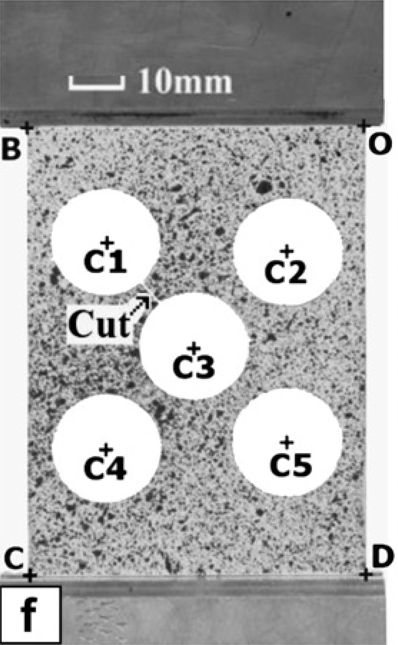
	X (mm)	Y (mm)
O	0	0
B	-62	0
C	-62	-82.5
D	0	-82.5
$C_{1}$	-47.5	-21.4
$C_{2}$	-14.0	-23.0
$C_{3}$	-31.5	-41.0
$C_{4}$	-47.7	-59.1
$C_{5}$	-14.5	-58.0

Figure 1: Geometry of the silicone sample, position of the holes and initial mesh.

Tested samples are deformed using a universal mechanical testing machine (MTS 4M) (see [36]). Dirichlet boundary conditions are imposed on the bottom edge of the dumbell silicone sample. On the left and right boundaries, we impose a homogeneous Neumann boundary condition (${\bf F}={\bf 0}$). In the experiment, the following Neumann boundary condition is imposed on the top edge: ${\bf F}=\left(f_{A}/(b_{0}\times e_{0})\right){\bf n}$ such that $\int_{\Gamma_{N}}{\bf F}\cdot{\bf n}\,\mathrm{ds}=20$ N. This force implies an observed vertical displacement of 57.3mm. In the simulations, we do it the other way round: we fix the bottom and we impose a displacement of 57.3mm on the top. We guess the corresponding traction force on the top boundary. Thus,we will consider the following quantities of interest

$$Q(\bm{u},\bm{p})=\int_{\mbox{top}}(\bm{\Pi}(\bm{u})\cdot\bm{N})\cdot\bm{N}\mathrm{d}s,$$

where the integral is taken on the top of the silicon band.

Table 1 recalls the value of the constitutive parameters used in the simulations. In Table 2, we compare the model and discretisation error for the constitutive laws of Mooney-Rivlin (2), Gent (3) and Haine-Wilson (4), respectively, for the quantity $Q$. The model error corresponds to the relative error between a very fine FEM solution $\bm{u}_{\mbox{fine}}$ and the experimental quantity of interest. The discretization error corresponds to the relative error between the computed solution on the current mesh and the computed solution on a very fine mesh, i.e.

$$\mbox{model error}=\dfrac{|Q(\bm{u}_{\mbox{fine}})-20|}{20}\mbox{ and discr. error}=\dfrac{|Q(\bm{u}_{h})-Q(\bm{u}_{\mbox{fine}})|}{Q(\bm{u}_{\mbox{fine}})}.$$

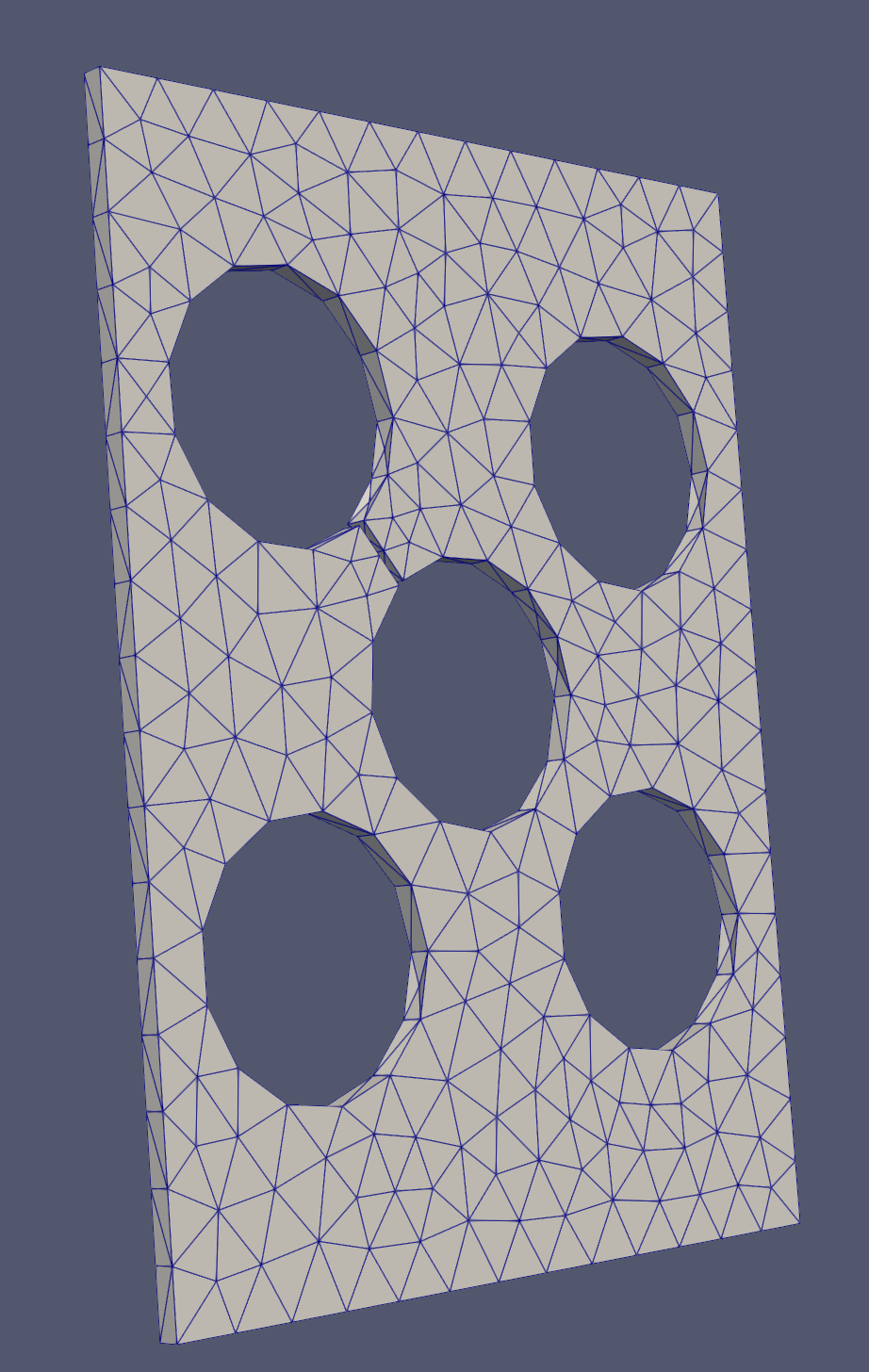
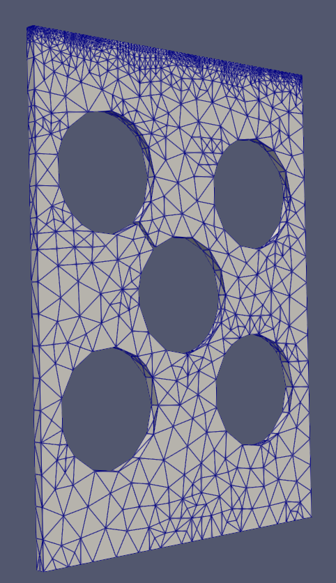
The parameters of each law have been estimated from [36] and are provided in Table 1. We give in Figure 3 the refined mesh in the case of the Haine-Wilson law (left) and the deformed geometry when we apply the load (right). We remark that the refinement occurs mainly on the top the silicone where is localised the quantity of interest but also near the holes.

Mooney	$C_{10}=0.14$	$C_{01}=0.023$
Gent	$E=0.97$	$J_{m}=13$
Haines-Wilson	$C_{10}=0.14$	$C_{20}=-0.0026$	$C_{30}=0.0038$
	$C_{01}=0.033$	$C_{02}=0.00095$	$C_{11}=-0.0049$

Table 1: First test case (silicone sample). Values of the constitutive parameters of each hyperelastic law, following [36].

Mooney-Rivlin			Gent			Haine Wilson
Nb	Model	Discr.	Nb	Model	Discr.	Nb	Model	Discr.
Cells	Error	Error	Cells	Error	Error	Cells	Error	Error
1333		7.0%	1333		9.6%	1333		8.0%
1664		8.1%	1654		10.4%	1706		8.8%
3047		7.2%	3281		9.1%	3441		7.8%
5307	17.0%	4.3%	5414	2.1%	5.9%	5692	0.5%	4.6 %
9426		3.0%	9947		3.7%	10383		2.9 %
18118		2.3%	18088		2.6%	19489		2.0%
33982		1.9%	34883		2.0%	38466		1.8%

Table 2: First test case (silicone sample). Relative model and discretisation error of the quantity of interest $Q_{1}$ with respect to the number of cells. The model error is computed thanks to the experimental data.

Figure 2: lar

Figure 3: First test case (silicone sample). Refined mesh for the Haine-Wilson model (left); Deformed geometry (right)

Figure 4: First test case (silicone sample). Relative error of discretisation (left) and efficiency of the estimator (right).

3.2 Second test case : Human heel

A pressure ulcer (PU) is a wound stemming from excessive loads on biological soft tissues which leads to ischemia, which in turn triggers tissue necrosis. Two fifth of the patients taken in charge by a reanimation unit or in a geriatric unit will develop a PU. 40% of those ulcers are located at the posterior part of the heel because the patient stays for hours lying on his back without moving [43]. This condition is often followed by amputation of part of the foot. The high prevalence of the pathology is the motivation behind the recent development of PU prevention strategies. Some of these approaches resort to personalized biomechanical modeling of the patient’s soft tissues, where tissue compression is numerically predicted based on the loads measured underneath the bedridden patient’s heels. The current consensus in the PU prevention community is that PU risk assessment should be based on an indicator of tissue suffering derived from the Von Mises stress, see [31]. Thus, a personalized biomechanical model should be able to predict the onset of a PU by continuously monitoring this quantity of interest, and by triggering an alarm if the risk exceeds a pre-defined threshold.

The accuracy of such prediction not only highly depends on the accuracy of the determined mechanical properties of the heel tissue, on the correct boundary conditions used in the simulation, but also on the numerical method (here the FEM) which is capable to solve the problem in a way that the error is controlled.

Figure 5 shows a heel tissue model used in our simulation. Its orientation corresponds to the situation when the patient is on bed. Boundary conditions used are shown in Figure 6. We consider Von Mises stress is a good factor to predict the tissue damage. A region in which we consider the heel tissue is vulnerable is shown by cyan colour in Figure 6(b). Our quantity of interest is thus expressed through the first Piola-Kirchhoff stress tensor $\bm{\Pi}$ over the domain of interest $\omega$, as

$$Q(\bm{\Pi}(\bm{u},\bm{p}))=\int_{\omega}\sqrt{\frac{1}{2}\left((\bm{\Pi}_{11}-\bm{\Pi}_{22})^{2}+(\bm{\Pi}_{22}-\bm{\Pi}_{33})^{2}+(\bm{\Pi}_{33}-\bm{\Pi}_{11})^{2}+3(\bm{\Pi}_{12}^{2}+\bm{\Pi}_{21}^{2}+\bm{\Pi}_{23}^{2}+\bm{\Pi}_{32}^{2}+\bm{\Pi}_{31}^{2}+\bm{\Pi}_{13}^{2})\right)}.$$ (11)

The heel tissue is supposed to behave like an incompressible hyperelastic material with the mechanical properties: Mooney-Rivlin with $C_{10}=16.6kPa$ and $C_{01}=0$ (see [44]).

Figure 5: A part of a heel tissue model used in simulations in which its orientation corresponds to the situation when the patient is on bed.

(a)

(b)

Figure 6: The heel tissue is considered to be fixed on the surface which has contact with the calcaneum, and on the upper surface, shown by gray colour in (6(a)); the tissue surface where a pressure is applied is shown by red colour, whereas a region of interest is also shown by red colour (6(b)).

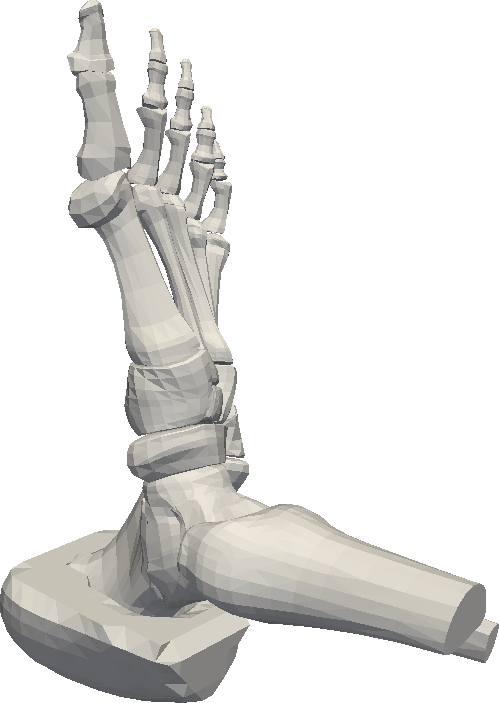
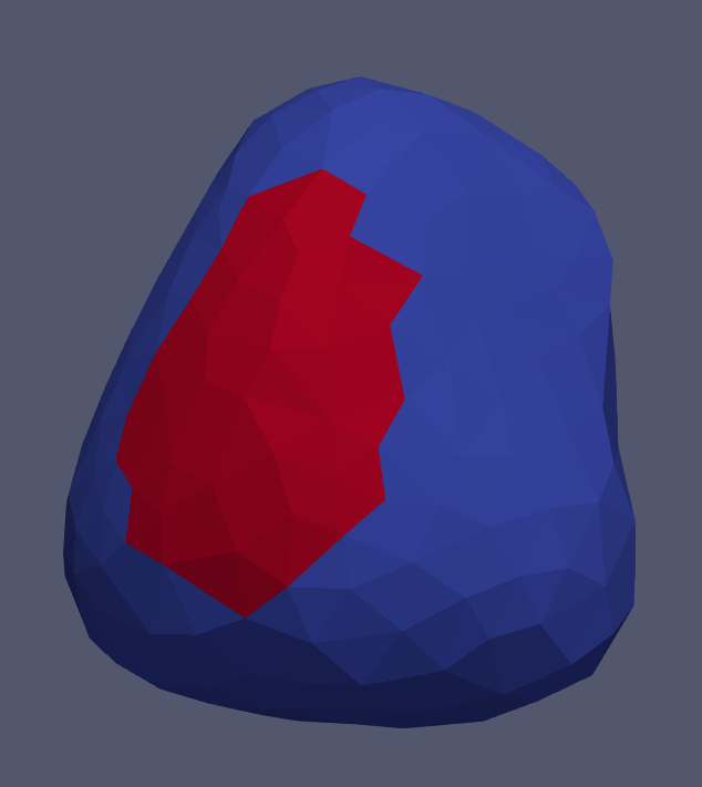
Figure 7 shows the convergence of the error estimator under both uniform and adaptive refinements. It is observed again that using adaptive refinement scheme is more advantageous than the uniform one since the corresponding error converges with higher rate. Refinement patterns are shown in Figure 8.

Figure 7: Second test case (Human heel undergone surface pressure). Relative error of discretisation (left) and efficiency of the estimator (right).

(a)

(b)

(c)

(d)

(e)

(f)

(g)

(h)

Figure 8: Second test case (Human heel undergone surface pressure). From the back, initial mesh (8(a)), adaptive mesh obtained after the first iteration of refinement (8(b)), after the second iteration of refinement (8(c)), the final mesh obtained after the $3th$ iteration of refinement (8(d)). The same meshes from the front (8(e))-(8(h)).

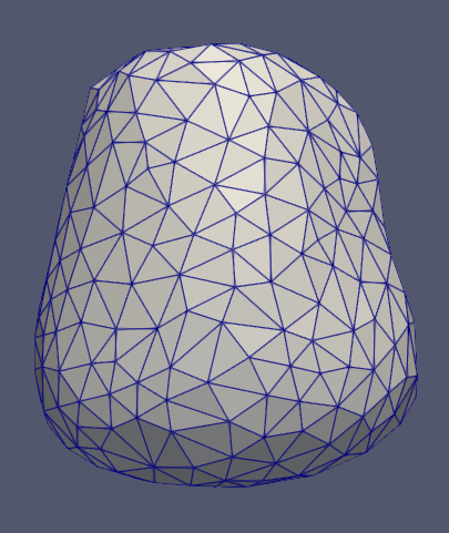
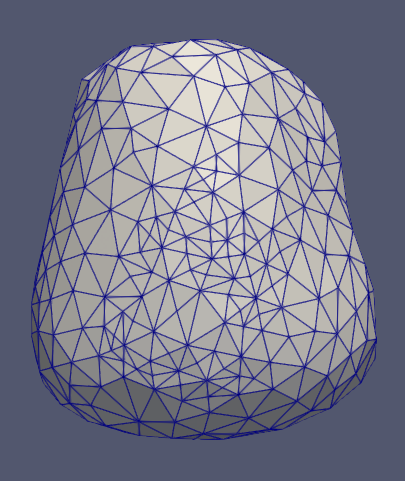
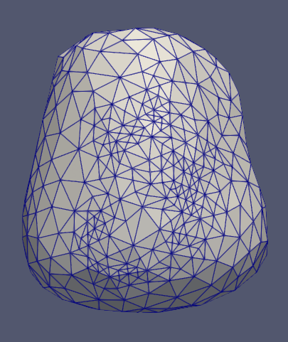
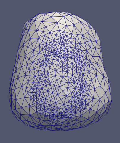
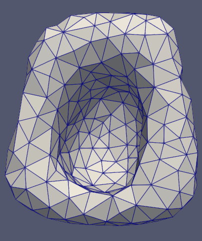
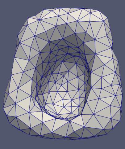
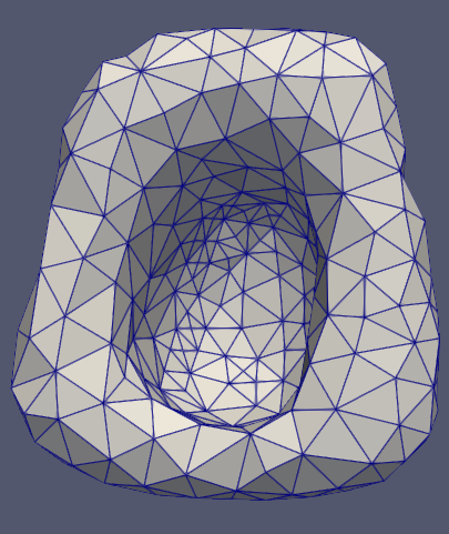
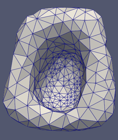
We remark that the algorithm refine in the lower part of the heel which is in coherence with [56, 18, 52, 33]. These zones correspond to the onset of pressure ulcers (see [53]). The added value of our DWR-driven adaptative meshing is that it automatically refines according to a quantity of interest. It not only optimises locally in the region of interest but also takes into account the far-field / global errors that contribute.

4 Discussion

We summarize below our main achievements, discuss their current limitations and suggest some perspectives.

4.1 Main achievements

We illustrate in this paper the feasibility of carrying out mesh refinement in modern finite element environments such as FEniCS, driven by a goal oriented error estimate, to improve the accuracy of an arbitrary user-defined quantity of interest. This is done for a three-dimensional nonlinear problem that involves incompressible hyperelasticity. This model is of common use in the biomechanics community. Notably, large displacements and large strain are taken into account. Furthermore, there is no difficulty to incorporate incompressibility.

The prediction outcome of the simulations has been confronted to experimental measurements on silicone sheets. Validation and verification of simulations in computational biomechanics is a complicated issue, since measurements on real patients and real clinical situations lack of precision and reproductibility. Indeed, some difficulties arise to control and know accurately all the relevant parameters. Though they are of course not identical as human soft tissues, materials such as silicone are interesting, since the numerical model can be calibrated with precision and numerical simulations can be confronted to measurements. However, it is still very difficult to find some published material for this purpose, and we took advantage of the study of Meunier et al [36]. In addition, let us emphasize the following points

1. The test with the silicone sample provides extra information about the modelling error, in the sense it also quantifies the predictive power of the constitutive law.

2. When the mesh is too coarse, the discretization error is of the same magnitude of this modelling error.

3. With adaptive mesh refinement, the discretization error can be controlled and driven below a given threshold that makes it negligible, without having to overrefine the mesh.

4. Another example close to clinical biomechanics has been carried out on a three-dimensional complex patient-specific geometry of the heel.

5. The method is easy to implement in an environment such as FEniCS, and the scripts are freely available. They can be transposed without much difficulty to other similar environments such as SONICS[35], GetFEM++[47], FreeFEM++[25] or SciKit-FEM[24].

6. Notably the automatic differentiation tools now available in modern finite element software facilitate a lot the assembly of the dual problem. Solving the, linear, dual problem remains inexpensive in comparison with the total solution procedure needed for the nonlinear problem. Last but not least, the solution of this dual problem is the basis of counterintuitive refinement strategies, much more efficient than adhoc refinement.

4.2 Current limitations

Let us point out as well some limitations of the proposed methodogy:

1. The dual solution needs to be approximated, and when the same finite element spaces are used for the primal and dual problem, an extra extrapolation step needs to be carried out. The accuracy of this procedure may be quantified more precisely and improved. In practice it has revealed small effect and does not hamper the efficiency of the methodology, but better results may even be expected if this point is improved. Another possibility is to use higher order spaces for the dual problem, but this solution is much more expensive.

2. The adjoint problem, though it is linear, inherits its coefficients from the nonlinear primal problem. In specific situations, it may be ill conditionned and this issue would need further investigation.

3. From the representation formula (9) of Becker and Rannacher at the core of the error estimate, we neglect the linearization error. Of course, this one is complicated to estimate in general and is expected to be small, but this point may deserve to be studied more carefully in the future.

4. Reference solutions are computed solutions on fine meshes or eventually experimental data. It could be interesting also to test the methodology with manufactured solutions in hyperelasticity [42, 7, 13].

4.3 Perspectives

To decrease the computation time, it can be interesting to perfom the refinement at each step throughout the loading. It can be significant when considering non-linear problems. A stimulating perspective would be first to combine the current methodology with techniques for model selection, and to estimate more systematically the model error. Also, since, for patient-specific biomechanics, some data can be used for (possibly) real time parameter calibration, it would be interesting to take advantage of the flexibility of the current framework to account for parameter calibration, as already done in Becker & Vexler [4, 5] for a general setting. Another point would consist in making the methodology available in software that are of common use in the whole biomechanics community. More generally, a perspective can be the comparison of the model et discretisation error with the errors coming from the geometry, the parameters of the model and the forces applied on the organ.

5 Acknowledgements

The authors thank Roland Becker, Jacques Ohayon, Yohan Payan and Yves Renard for their advices. They also thank the AMIES for its support, particularly Magalie Fredoc, Antoine Lejay and Christophe Prudhomme.

Appendix A Expression of the estimator and algorithms

We give below for each cell-wise contribution:

$$\eta_{K}=\left|\int_{K}\bm{R}_{\bm{u}}\cdot(\bm{z}_{h}-I_{h}(E_{h}(\bm{z}_{h}))\mathrm{d}\Omega+\int_{K}\bm{R}_{\bm{p}}\cdot(\bm{p}_{h}-I_{h}(E_{h}(\bm{p}_{h}))\mathrm{d}\Omega+\int_{\partial K}\bm{J}\cdot(\bm{z}_{h}-I_{h}(E_{h}(\bm{z}_{h}))\mathrm{d}\gamma\right|$$ (12)

with, $E_{h}$ and $I_{h}$ are resp. the extrapolation (see [48]) and the Lagrange interpolation, the interior residual

$$\bm{R}_{\bm{u}}=\bm{B}+\mathrm{div}\,\bm{\Pi}(\bm{u}_{h})\mbox{ and }\bm{R}_{\bm{p}}=\det(\bm{C})-1$$

and the stress jump

$$\bm{J}=\begin{cases}-\frac{1}{2}[[\bm{\Pi}(\bm{u}_{h})]]&\text{ if }\gamma\not\subset\Gamma,\\ \bm{T}-\bm{\Pi}({\bf u}_{h})\cdot\bm{N}&\text{ if }\gamma\subset\Gamma_{N},\\ \bm{0}&\text{ if }\gamma\subset\Gamma_{D}.\end{cases}$$

The jump can be defined for a function $\bm{v}_{h}$ on a facet $F$ between two cells $K$ and $K^{\prime}$ by $[[\bm{v}_{h}]]=\bm{v}_{h|K}\cdot n_{K}+\bm{v}_{h|K^{\prime}}\cdot n_{K^{\prime}}$, where $n_{K}$ and $n_{K^{\prime}}$ are the normal of $K$ and $K^{\prime}$ on $F$.

Algorithm 1 Algorithm for mesh refinement

Select an initial triangulation $mesh_{i}$ of the domain $\Omega$

Guest solution $(\bm{u}_{i}^{(0)},\bm{p}_{i}^{(0)})$

while $\sum_{K}\eta_{K}>\epsilon$ do

     $F(\bm{u}_{i},\bm{p}_{i};\bm{v},\bm{q})\leftarrow A(\bm{u}_{i},\bm{p}_{i};\bm{v},\bm{q})-L(\bm{v},\bm{q})$

     $\bm{u}_{i},\bm{p}_{i}\leftarrow$ NewtonMethod $(F(\bm{u}_{i},\bm{p}_{i};\bm{v},\bm{q}),(\bm{u}_{i}^{(0)},\bm{p}_{i}^{(0)}))$ $\triangleright$ Problem (5), see Algo 2

     $\bm{z}_{i},\bm{w}_{i}\leftarrow$ DualProblem $(\bm{u}_{i},\bm{p}_{i},Q)$ $\triangleright$ Problem (7), see Algo 3

     $\eta_{K}\leftarrow$ ComputeEstimator $(\bm{u}_{i},\bm{p}_{i},\bm{z}_{i},\bm{w}_{i})$

     markedElements $\leftarrow$ DorflerMarking $(\eta_{K},\alpha)$ $\triangleright$ See Algo Algorithm 4

     $mesh_{i}\leftarrow mesh_{i}$.refine(markedElements)

     Compute $\sum_{K}\eta_{K}$

end while

Algorithm 2 Solving a non-linear problem: NewtonMethod $(F(\bm{u}_{i}^{(0)},\bm{v}),\bm{u}_{i}^{(0)})$

$(\bm{u}_{k},\bm{p}_{k})=(\bm{u}_{i}^{(0)},\bm{p}_{i}^{(0)})$

while $\lvert(\delta\bm{u},\delta\bm{p})\rvert>\epsilon$ do

     $F^{\prime}(\bm{u}_{k};\delta\bm{u},\bm{v})=-F(\bm{u}_{k};\bm{v})$ $\triangleright$ Solve for $\delta\bm{u}$

     $(\bm{u}_{k+1},\bm{p}_{k+1})\leftarrow(\bm{u}_{k}+\delta\bm{u},\bm{p}_{k}+\delta\bm{p})$ $\triangleright$ Update the solution

     Compute $\lvert(\delta\bm{u},\delta\bm{p})\rvert$

end while

Algorithm 3 Solving the dual problem: DualProblem $(\bm{u}_{i},Q)$

Compute $A^{\prime}(\bm{u}_{i},\bm{p}_{i}|\bm{z}_{i},\bm{w}_{i};\bm{v},\bm{q})$

Compute $Q^{\prime}(\bm{u}_{i},\bm{p}_{i};\bm{v},\bm{q})$

$(\bm{z}_{i},\bm{w}_{i})\leftarrow$ solve $(A^{\prime}(\bm{u}_{i},\bm{p}_{i}|\bm{z}_{i},\bm{w};\bm{v},\bm{q})=Q^{\prime}(\bm{u}_{i},\bm{p}_{i};\bm{v},\bm{q}))$ $\triangleright$ Solve the linear system

Algorithm 4 Mark elements after Dörfler strategy by providing a element-wise estimator $\eta_{K}=[\eta_{K_{1}},\eta_{K_{2}},\dots\eta_{K_{N}}]$, and $0<\alpha<1$ a parameter which characterises the marking rate: the smaller the value of $\alpha$ is, the fewer the number of elements will be marked: DorflerMarking $(\eta_{K},\alpha)$

Sort the elements $K_{i}$ after descending order of the corresponding estimator $\eta_{K_{i}}$

Mark the first $M$ elements such that

$$\mathrm{markedElements}\leftarrow\min\left\{M\in N\>\middle|\>\sum\limits_{i=1}^{M}\eta_{K_{i}}\geq\alpha\sum_{i=1}^{N}\eta_{K_{i}}\right\}.$$

References

- [1] M. Ainsworth and J. T. Oden. A posteriori error estimation in finite element analysis. Pure and Applied Mathematics. Wiley-Interscience, New York, 2000.
- [2] R. Becker and R. Rannacher. A feed-back approach to error control in finite element methods: basic analysis and examples. East-West Journal of Numerical Mathematics, 4(4):237–264, 1996.
- [3] R. Becker and R. Rannacher. An optimal control approach to a posteriori error estimation in finite element methods. Acta Numerica, 10:1–102, 2001.
- [4] R. Becker and B. Vexler. A posteriori error estimation for finite element discretization of parameter identification problems. Numerische Mathematik, 96(3):435–459, 2004.
- [5] R. Becker and B. Vexler. Mesh refinement and numerical sensitivity analysis for parameter calibration of partial differential equations. Journal of Computational Physics, 206(1):95–110, 2005.
- [6] A. Bijar, P.-Y. Rohan, P. Perrier, and Y. Payan. Atlas-based automatic generation of subject-specific finite element tongue meshes. Annals of Biomedical Engineering, 44(1):16–34, 2016.
- [7] M. Blaise, F. Chouly, and P.-Y. Rohan. A few remarks about the computer implementation and the verification of some hyperelastic constitutive laws and an illustration with the mechanical response of an artery. hal-03637834, Apr. 2022.
- [8] S. Buchaillard, M. Brix, P. Perrier, and Y. Payan. Simulations of the consequences of tongue surgery on tongue mobility: implications for speech production in post-surgery conditions. The International Journal of Medical Robotics and Computer Assisted Surgery, 3(3):252–261, 2007.
- [9] M. Bucki, C. Lobos, Y. Payan, and N. Hitschfeld. Jacobian-based repair method for finite element meshes after registration. Engineering with Computers, 27(3):285–297, 2011.
- [10] H. P. Bui, S. Tomar, H. Courtecuisse, M. Audette, S. Cotin, and S. P. Bordas. Controlling the error on target motion through real-time mesh adaptation: Applications to deep brain stimulation. International Journal for Numerical Methods in Biomedical Engineering, pages e2958–n/a, 2017. e2958 cnm.2958.
- [11] H. P. Bui, S. Tomar, H. Courtecuisse, S. Cotin, and S. P. A. Bordas. Real-time error control for surgical simulation. IEEE Transactions on Biomedical Engineering, 65(3):596–607, March 2018.
- [12] T. J. Carter, M. Sermesant, D. M. Cash, D. C. Barratt, C. Tanner, and D. J. Hawkes. Application of soft tissue modelling to image-guided surgery. Medical Engineering & Physics, 27(10):893 – 909, 2005. Advances in the finite element modelling of soft tissue deformation.
- [13] É. Chamberland, A. Fortin, and M. Fortin. Comparison of the performance of some finite element discretizations for large deformation elasticity problems. Computers & Structures, 88(11-12):664–673, 2010.
- [14] H. Courtecuisse, J. Allard, P. Kerfriden, S. P. A. Bordas, S. Cotin, and C. Duriez. Real-time simulation of contact and cutting of heterogeneous soft-tissues. Medical Image Analysis, 18(2):394–410, 2014.
- [15] W. Dörfler. A convergent adaptive algorithm for Poisson’s equation. SIAM Journal on Numerical Analysis, 33(3):1106–1124, 1996.
- [16] M. Duprez, S. P. A. Bordas, M. Bucki, H. P. Bui, F. Chouly, V. Lleras, C. Lobos, A. Lozinski, P.-Y. Rohan, and S. Tomar. Quantifying discretization errors for soft tissue simulation in computer assisted surgery: a preliminary study. Applied Mathematical Modelling, 77(part 1):709–723, 2020.
- [17] M. Duprez, A. Lejeune, F. Chouly, S. Bordas, and B. P. Huu. DWR-hyperelastic-soft-tissue. figshare, 4 2023.
- [18] A. Gefen. The biomechanics of heel ulcers. Journal of Tissue Viability, 19(4):124–131, 2010.
- [19] A. N. Gent. A New Constitutive Relation for Rubber. Rubber Chemistry and Technology, 69(1):59–61, 03 1996.
- [20] M. B. Giles and E. Süli. Adjoint methods for PDEs: a posteriori error analysis and postprocessing by duality. Acta Numerica, 11:145–236, 2002.
- [21] O. A. González-Estrada, E. Nadal, J. J. Ródenas, P. Kerfriden, S. P. A. Bordas, and F. J. Fuenmayor. Mesh adaptivity driven by goal-oriented locally equilibrated superconvergent patch recovery. Computational Mechanics, 53(5):957–976, 2014.
- [22] B. N. Granzow, A. A. Oberai, and M. S. Shephard. Adjoint-based error estimation and mesh adaptation for stabilized finite deformation elasticity. Computer Methods in Applied Mechanics and Engineering, 337:263–280, 2018.
- [23] T. Grätsch and K.-J. Bathe. A posteriori error estimation techniques in practical finite element analysis. Computers & Structures, 83(4):235–265, 2005.
- [24] T. Gustafsson and G. D. Mcbain. scikit-fem: A python package for finite element assembly. Journal of Open Source Software, 5(52):2369, 2020.
- [25] F. Hecht. New development in freefem++. Journal of Numerical Mathematics, 20(3-4):251–266, 2012.
- [26] V. Heuveline and R. Rannacher. Duality-based adaptivity in the hp-finite element method. Journal of Numerical Mathematics, 11:95–113, 2003.
- [27] A. James, A. Green, and G. Simpson. Strain energy functions of rubber. i. characterization of gum vulcanizates. Journal of Applied Polymer Science, 19(7):2033–2058, 1975.
- [28] P. Kranke, L. H Eberhart, T. J Gan, N. Roewer, and M. R Tramèr. Algorithms for the prevention of postoperative nausea and vomiting: An efficacy and efficiency simulation. European Journal of Anaesthesiology, 24:856–67, 10 2007.
- [29] U. Kühnapfel, H. Çakmak, and H. Maaß. Endoscopic surgery training using virtual reality and deformable tissue simulation. Computers & Graphics, 24(5):671 – 682, 2000.
- [30] F. Larsson, P. Hansbo, and K. Runesson. Strategies for computing goal-oriented a posteriori error measures in non-linear elasticity. Internat. J. Numer. Methods Engrg., 55(8):879–894, 2002.
- [31] S. Loerakker, E. Manders, G. J. Strijkers, K. Nicolay, F. P. Baaijens, D. L. Bader, and C. W. Oomens. The effects of deformation, ischemia, and reperfusion on the development of muscle damage during prolonged loading. Journal of Applied Physiology, 111(4):1168–1177, 2011.
- [32] V. Luboz, M. Bailet, C. Boichon Grivot, M. Rochette, B. Diot, M. Bucki, and Y. Payan. Personalized modeling for real-time pressure ulcer prevention in sitting posture. Journal of Tissue Viability, 27(1):54–58, 2018.
- [33] V. Luboz, A. Perrier, M. Bucki, B. Diot, F. Cannard, N. Vuillerme, and Y. Payan. Influence of the calcaneus shape on the risk of posterior heel ulcer using 3d patient-specific biomechanical modeling. Annals of Biomedical Engineering, 43:325–335, 2015.
- [34] Y. Maday and A. T. Patera. Numerical analysis of a posteriori finite element bounds for linear functional outputs. Mathematical Models and Methods in Applied Sciences, 10(5):785–799, 2000.
- [35] A. Mazier, S. E. Hadramy, J.-N. Brunet, J. S. Hale, S. Cotin, and S. Bordas. Sonics: Develop intuition on biomechanical systems through interactive error controlled simulations. arXiv preprint arXiv:2208.11676, 2022.
- [36] L. Meunier, G. Chagnon, D. Favier, L. Orgéas, and P. Vacher. Mechanical experimental characterisation and numerical modelling of an unfilled silicone rubber. Polymer Testing, 27(6):765–777, 2008.
- [37] B. Mielczarek and J. Uziałlko-Mydlikowska. Application of computer simulation modeling in the health care sector: a survey. SIMULATION, 88(2):197–216, 2012.
- [38] M. Mooney. A theory of large elastic deformation. Journal of Applied Physics, 11(9):582–592, 1940.
- [39] R. H. Nochetto, K. G. Siebert, and A. Veeser. Theory of adaptive finite element methods: an introduction. In Multiscale, nonlinear and adaptive approximation, pages 409–542. Springer, Berlin, 2009.
- [40] J. Oden and S. Prudhomme. Goal-oriented error estimation and adaptivity for the finite element method. Computers & Mathematics with Applications, 41(5):735 – 756, 2001.
- [41] M. Paraschivoiu, J. Peraire, and A. T. Patera. A posteriori finite element bounds for linear-functional outputs of elliptic partial differential equations. Computer Methods in Applied Mechanics and Engineering, 150(1-4):289–312, 1997. Symposium on Advances in Computational Mechanics, Vol. 2 (Austin, TX, 1997).
- [42] Y. Payan and J. Ohayon. Biomechanics of living organs: hyperelastic constitutive laws for finite element modeling. Academic Press Series in Biomedical Engineering. Elsevier, 2017.
- [43] T. Perneger, C. Heliot, A. Rae, F. Borst, and J. Gaspoz. Hospital acquired pressure ulcers. risk factors and use of preventive devices. Arch Intern Med, 158(17):1940 – 1945, 1998.
- [44] A. Perrier, V. Luboz, M. Bucki, F. Cannard, N. Vuillerme, and Y. Payan. Biomechanical modelling of the foot. In Y. Payan and J. Ohayon, editors, Biomechanics of Living Organs: Hyperelastic Constitutive Laws for Finite Element Modeling, pages 545–563. Elsevier, 2017.
- [45] D. Perrin, P. Badel, L. Orgéas, C. Geindreau, A. Dumenil, J.-N. Albertini, and S. Avril. Patient-specific numerical simulation of stent-graft deployment: validation on three clinical cases. Journal of Biomechanics, 48(10):1868–1875, 2015.
- [46] S. Prudhomme and J. T. Oden. On goal-oriented error estimation for elliptic problems: application to the control of pointwise errors. Computer Methods in Applied Mechanics and Engineering, 176(1-4):313–331, 1999. New advances in computational methods (Cachan, 1997).
- [47] Y. Renard and K. Poulios. Getfem: Automated fe modeling of multiphysics problems based on a generic weak form language. ACM Transactions on Mathematical Software (TOMS), 47(1):1–31, 2020.
- [48] M. E. Rognes and A. Logg. Automated goal-oriented error control I: Stationary variational problems. SIAM Journal on Scientific Computing, 35(3):C173–C193, 2013.
- [49] A. Romo, P. Badel, A. Duprey, J.-P. Favre, and S. Avril. In vitro analysis of localized aneurysm rupture. Journal of Biomechanics, 47(3):607–616, 2014.
- [50] H. Schmidt, F. Galbusera, A. Rohlmann, T. Zander, and H.-J. Wilke. Effect of multilevel lumbar disc arthroplasty on spine kinematics and facet joint loads in flexion and extension: a finite element analysis. European Spine Journal, 21(5):663–674, 2012.
- [51] D. Selle, B. Preim, A. Schenk, and H.-O. Peitgen. Analysis of vasculature for liver surgical planning. IEEE Transactions on Medical Imaging, 21(11):1344–1357, Nov 2002.
- [52] H. Shaulian, A. Gefen, D. Solomonow-Avnon, and A. Wolf. Finite element-based method for determining an optimal offloading design for treating and preventing heel ulcers. Computers in Biology and Medicine, 131:104261, 2021.
- [53] W. A. Traa, M. C. van Turnhout, K. M. Moerman, J. L. Nelissen, A. J. Nederveen, G. J. Strijkers, D. L. Bader, and C. W. Oomens. Mri based 3d finite element modelling to investigate deep tissue injury. Computer methods in biomechanics and biomedical engineering, 21(14):760–769, 2018.
- [54] O. Trabelsi, F. M. Davis, J. F. Rodriguez-Matas, A. Duprey, and S. Avril. Patient specific stress and rupture analysis of ascending thoracic aneurysms. Journal of Biomechanics, 48(10):1836–1843, 2015.
- [55] S. Urcun, D. Baroli, P.-Y. Rohan, W. Skalli, V. Lubrano, S. P. Bordas, and G. Sciume. Non-operable glioblastoma: proposition of patient-specific forecasting by image-informed poromechanical model. Brain Multiphysics, page 100067, 2023.
- [56] W. van Zwam, M. C. van Turnhout, and C. W. Oomens. Risk factors for developing heel ulcers for bedridden patients: A finite element study. Clinical Biomechanics, 78:105094, 2020.
- [57] M. W. Vannier, J. L. Marsh, and J. O. Warren. Three dimensional ct reconstruction images for craniofacial surgical planning and evaluation. Radiology, 150(1):179–184, 1984. PMID: 6689758.
- [58] R. Verfürth. A posteriori error estimation techniques for finite element methods. Oxford University Press, Oxford, 2013.
- [59] S. K. Warfield, F. Talos, A. Tei, A. Bharatha, A. Nabavi, M. Ferrant, P. McL. Black, F. A. Jolesz, and R. Kikinis. Real-time registration of volumetric brain mri by biomechanical simulation of deformation during image guided neurosurgery. Computing and Visualization in Science, 5(1):3–11, Jul 2002.
- [60] J. P. Whiteley and S. J. Tavener. Error estimation and adaptivity for incompressible hyperelasticity. International Journal for Numerical Methods in Engineering, 99(5):313–332, 2014.
- [61] T. E. Yankeelov, N. Atuegwu, D. Hormuth, J. A. Weis, S. L. Barnes, M. I. Miga, E. C. Rericha, and V. Quaranta. Clinically relevant modeling of tumor growth and treatment response. Science Translational Medicine, 5(187):187ps9–187ps9, 2013.
- [62] O. Zienkiewicz and J. Zhu. The superconvergent patch recovery (spr) and adaptive finite element refinement. Computer Methods in Applied Mechanics and Engineering, 101(1):207–224, 1992.