UniTS: Building a Unified Time Series Model

Abstract

Foundation models, especially LLMs, are profoundly transforming deep learning. Instead of training many task-specific models, we can adapt a single pretrained model to many tasks via few-shot prompting or fine-tuning. However, current foundation models apply to sequence data but not to time series, which present unique challenges due to the inherent diverse and multi-domain time series datasets, diverging task specifications across forecasting, classification and other types of tasks, and the apparent need for task-specialized models. We developed UniTS, a unified time series model that supports a universal task specification, accommodating classification, forecasting, imputation, and anomaly detection tasks. This is achieved through a novel unified network backbone, which incorporates sequence and variable attention along with a dynamic linear operator and is trained as a unified model. Across 38 multi-domain datasets, UniTS demonstrates superior performance compared to task-specific models and repurposed natural language-based LLMs. UniTS exhibits remarkable zero-shot, few-shot, and prompt learning capabilities when evaluated on new data domains and tasks. The source code and datasets are available at https://github.com/mims-harvard/UniTS.

1 Introduction

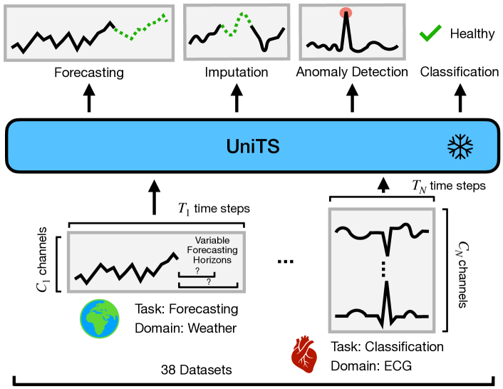
Figure 1: UniTS is a unified time series model that can process various tasks across multiple domains with shared parameters and does not have any task-specific modules.

Machine learning community has long pursued the development of unified models capable of handling multiple tasks. Such unified and general-purpose models have been developed for language (Brown et al., 2020; Touvron et al., 2023) and vision (Rombach et al., 2022; Kirillov et al., 2023; Gao et al., 2023), where a single pretrained foundation model can be adapted to new tasks with little or no additional training via multi-task learning (Zhang & Yang, 2021), few-shot learning (Wang et al., 2020), zero-shot learning (Pourpanah et al., 2022), and prompt learning (Liu et al., 2022a).

However, general-purpose models for time series have been relatively unexplored. Time series datasets are abundant across many domains—including medicine (Goldberger et al., 2000b), engineering (Trindade, 2015), and science (Kaltenborn et al., 2023)—and are used for a broad range of tasks such as forecasting, classification, imputation, and anomaly detection. Current time series models, however, require either fine-tuning or specifying new task- and dataset-specific modules to transfer to new datasets and tasks, which can lead to overfitting, hinder few- or zero-shot transfer, and burden users.

Building a unified time series model presents unique challenges: 1) Multi-domain temporal dynamics: Unified models learn general knowledge by co-training on diverse data sources, but time series data present wide variability in temporal dynamics across domains (He et al., 2023). Further, time series data may have heterogeneous data representations such as the number of variables, the definition of sensors, and length of observations. Such heterogeneity in time series data hinders the use of unified models developed for other domains (Zhang et al., 2023). Therefore, a unified model must be designed and trained to capture general temporal dynamics that transfer to new downstream datasets, regardless of data representation. 2) Diverging task specifications: Common tasks on time series data have fundamentally different objectives. For example, forecasting entails predicting future values in a time series, akin to a regression problem, while classification is a discrete decision-making process made on an entire sample. Further, the same task across different datasets may require different specifications, such as generative tasks that vary in length and recognition tasks featuring multiple categories. Existing time series models (Zhou et al., 2023; Wu et al., 2023) define task-specific modules to handle each task, which compromises their adaptability to diverse types of tasks. A unified model must be able to adapt to changing task specifications from users. 3) Requirement for task-specific time series modules: Unified models employ shared weights across various tasks, enhancing their generalization ability. However, the distinct task-specific modules for each dataset in previous approaches require the fine-tuning of these modules. This process often demands finely adjusted training parameters as well as a moderate dataset size per task, hindering rapid adaptation to new tasks. Such a strategy contradicts the concept of a unified model designed to manage multiple tasks concurrently.

Present work. To address these challenges, we introduce UniTS, a unified time series model that processes various tasks with shared parameters without resorting to any task-specific modules. UniTS achieves competitive performance in trained tasks and can perform zero-shot inference on novel tasks without the need for additional parameters. UniTS addresses the following challenges: 1) Universal task specification with prompting: UniTS uses a prompting-based framework to convert various tasks into a unified token representation, creating a universal specification for all tasks. 2) Data-domain agnostic network: UniTS employs self-attention across both sequence and variable dimensions to accommodate diverse data shapes. We introduce a dynamic linear operator to model dense relations between data points in sequence of any length. As a result, UniTS can process multi-domain time series with diverse variables and lengths without the need to modify network structure. 3) Unified model with fully shared weights: Leveraging the universal task specification and data-domain agnostic network, UniTS has shared weights across tasks. To improve UniTS generalization ability, a unified masked reconstruction pretraining scheme is introduced to handle both generative and recognition tasks within a unified model.

On a challenging multi-domain/task setting, a single UniTS with fully shared weights successfully handles 38 diverse tasks, indicating its potential as a unified time series model. UniTS outperforms top-performing baselines (which require data and task-specific modules) by achieving the highest average performance and the best results on 27 out of the total 38 tasks. Additionally, UniTS can perform zero-shot and prompt-based learning. It excels in zero-shot forecasting for out-of-domain data, handling new forecasting horizons and numbers of variables/sensors. For instance, in one-step forecasting with new lengths, UniTS outperforms the top baseline model, which relies on sliding windows, by 10.5%. In the prompt learning regime, a fixed, self-supervised pretrained UniTS is adapted to new tasks, achieving performance comparable to UniTS’s supervised counterpart; in 20 forecasting datasets, prompted UniTS outperforms the supervised version, improving MAE from 0.381 to 0.376. UniTS demonstrates exceptional performance in few-shot transfer learning, effectively handling tasks such as imputation, anomaly detection, and out-of-domain forecasting and classification without requiring specialized data or task-specific modules. For instance, UniTS outperforms the strongest baseline by 12.4% (MSE) on imputation tasks and 2.3% (F1-score) on anomaly detection tasks. Overall, UniTS shows the potential of unified models for time series and paves the way for generalist models in time series.

2 Related Work

Traditional time series modeling. Time series has been explored in the statistics and machine learning communities for many years (Hyndman & Athanasopoulos, 2018). Many neural architectures have been developed for specific time series tasks such as forecasting (Wu et al., 2021; Liu et al., 2021, 2023b), classification (Xiao et al., 2022; Lu et al., 2023; Liu et al., 2023c), anomaly detection (Ding et al., 2023; Li & Jung, 2023; Chen et al., 2023b), and imputation (Chen et al., 2023c; Kim et al., 2023; Ashok et al., 2024). These models are often trained with a strategy designed for one downstream task, often via supervised learning, on one dataset. Some work builds models specifically for irregularly-sampled time series (Zhang et al., 2022b; Chen et al., 2023d; Naiman et al., 2024). For a review on recent advancements in representation learning for time series, we refer the reader to a recent survey (Trirat et al., 2024).

Foundation models for general time series modeling. Foundation models are generally defined as models trained on broad data that can be adapted to diverse downstream tasks (Bommasani et al., 2021). Foundation models have become prevalent in many domains, including language modeling (Brown et al., 2020; Touvron et al., 2023) and computer vision (Liu et al., 2022b, 2023a; Kirillov et al., 2023). Recent works in time series have sought to develop similar capabilities to those observed in foundation models from other domains. Some works develop general pretraining strategies that facilitate effective transfer learning to new datasets and/or tasks. Common self-supervised pretraining approaches include predicting masked time segments (Nie et al., 2023; Zerveas et al., 2021; Dong et al., 2023; Lee et al., 2024), contrastive learning between augmented views of time series (Luo et al., 2023; Wang et al., 2023; Xu et al., 2024; Fraikin et al., 2024), or consistency learning between different representations of time series (Zhang et al., 2022c; Queen et al., 2023). Some works aim to build novel architectures that can capture diverse time series signals (Wu et al., 2023; Liu et al., 2024). One particular example of this is TimesNet (Wu et al., 2023), which uses multiple levels of frequency-based features obtained by Fourier transform, which is claimed to capture complex time series signals. Further, some studies have suggested to reprogram large language models to time series (Nate Gruver & Wilson, 2023; Chang et al., 2023; Zhou et al., 2023; Rasul et al., 2023; Jin et al., 2023; Cao et al., 2024). In GPT4TS (Zhou et al., 2023), the embedding layer, normalization layers, and output layer of GPT-2 (Radford et al., 2019) is selectively tuned for various time series tasks. However, they still need task-specific modules and tuning for each task, while UniTS supports various tasks without the need for task-specific modules.

Prompt learning. Prompt learning has emerged as a form of efficient task adaptation for large neural networks (Lester et al., 2021). Some methods rely on constructing prompts in the input domain of the model, such as text prompts for language models (Arora et al., 2023), while other methods tune soft token inputs to frozen language models (Li & Liang, 2021). Outside of language modeling, prompts have been used in computer vision (Radford et al., 2021; Zhang et al., 2022a; Chen et al., 2023a) and graph learning (Huang et al., 2023). One of the only instances of prompt learning in time series is TEMPO (Cao et al., 2024), which introduces a learned dictionary of prompts that are retrieved at inference time. However, these prompts are only used in the context of forecasting. Prompt learning for frozen UniTS enables adaptations to various new tasks beyond forecasting. Extended related works are presented in Appendix A.

3 Problem Formulation

Notation. We are given a set of multi-domain datasets $D=\{D_{i}|i=1,\ldots,n\}$, where each dataset $D_{i}$ can have a varying number of time series samples; samples can be of varying lengths and have varying numbers of sensors/variables. Each dataset is described as $D_{i}=(\mathcal{X}_{i},\mathcal{Y}_{i})$, where $\mathcal{X}_{i}$ denotes time series samples and $\mathcal{Y}_{i}$ specifies a task defined on $\mathcal{X}_{i}$. In this paper, we consider four common time series tasks: forecasting, classification, anomaly detection, and imputation. Further, each task type can be instantiated in numerous ways, e.g., short-term vs. long-term forecasting and classification with varying numbers of categories. We use $F(\mathcal{X}_{i},\theta)$ to denote a model with weights $\theta$ trained on $\mathcal{X}_{i}$, and $F(\mathcal{X},\theta)$ for a model trained on all datasets in $D$, i.e., $\mathcal{X}_{i}$ for all $i$. $\mathcal{\hat{X}}$ is an out-of-domain dataset collection not included in $\mathcal{X}$ and $\mathcal{\hat{Y}}$ is used to denote a new type of tasks not contained in $\mathcal{Y}$.

A time series sample is denoted as $\mathbf{x}\in\mathbb{R}^{l_{i}\times v}$, where $v$ and $l_{i}$ are the number of variables and sample/sequence length, respectively. We introduce several token types, i.e, sequence token $\mathbf{z}_{s}\in\mathbb{R}^{l_{s}\times v\times d}$, prompt token $\mathbf{z}_{p}\in\mathbb{R}^{l_{p}\times v\times d}$, mask token $\mathbf{z}_{m}\in\mathbb{R}^{1\times v\times d}$, CLS token $\mathbf{z}_{c}\in\mathbb{R}^{1\times v\times d}$, and category embeddings $\mathbf{z}_{e}\in\mathbb{R}^{k\times v\times d}$, each serving a specific purpose. $l_{s}$ and $l_{p}$ are the number of sequence and prompt tokens, $d$ is the feature dimension of tokens, and $k$ is the number of categories in a given classification task. The tokens sent to the network are denoted as $\mathbf{z}_{\text{in}}\in\mathbb{R}^{l\times v\times d}$, where $l$ is the sum of all tokens in the sequence dimension.

Unified time series model. Specialized time series models have been designed for specific tasks. Due to the diverse nature of time series and potentially diverging specifications of tasks (see Introduction), predominant models design task-specific networks to handle data/task differences and train separate models with elaborately tuned training parameters for each task (Liu et al., 2024; Wu et al., 2023).

Desiderata for a unified time series model. A unified time series model $F(\mathcal{X},\theta)$ is a single model with weights $\theta$ that are shared across all types of tasks and satisfies the following three desiderata:

• Multi-domain time series: While the unified model gathers information from all sources, the model $F$ must be agnostic with any input samples $\mathcal{X}$, given the diversity in sequence lengths $l_{in}$ and variable counts $v$ in time series sequence $x$ from various sources.

• Universal task specification: Instead of using separate task-specific modules, which hinder swift adaptation to new tasks, the unified model $F$ should adopt a universal task specification $F(\mathcal{X},\theta)\rightarrow\mathcal{Y}$ applicable across all type of tasks $\mathcal{Y}$.

• No task-specific modules (generalist): Sharing weights $\theta$ across tasks enables the unified model $F$ to handle multiple tasks simultaneously without requiring task-specific fine-tuning for each one. It contrasts with existing methods that typically train models on task-specific datasets, often involving elaborately tuned training parameters.

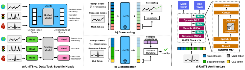
Figure 2: a) Compares UniTS to existing models, where UniTS model can process diverse inputs and achieve multiple time series tasks; previous models require separate modules for different tasks and input datasets. b) UniTS for forecasting; input is tokenized as described in-text and mask tokens are un-patchified to infer the forecast horizon. c) UniTS for classification; a CLS token is used to represent class information, and then compared to category tokens to get prediction class. d) Architecture of UniTS model.

Problem statement (UniTS). Realizing the above desiderata, UniTS incorporates multi-task, zero-shot, few-shot, and prompt learning. Multi-task learning: UniTS utilizes a single model $F(\theta)$ for multiple tasks $\mathcal{Y}$ across diverse data sources $\mathcal{X}$ in a diverse dataset collection, eliminating the need for task-specific fine-tuning. This is formalized as $F(\mathcal{X},\theta)\rightarrow\mathcal{Y}$. Multi-task learning showcases the flexibility of model in learning from and applying knowledge across different domains and tasks. Zero-shot learning: UniTS has zero-shot learning ability where model $F(\mathcal{X},\theta)$ trained on all datasets in $D$ is tested on multiple types of new tasks that are not trained for, i.e. $F(\mathcal{X},\theta)\rightarrow\mathcal{\hat{X}},\mathcal{\hat{X}}\notin\mathcal{X}$. New tasks for zero-shot learning include long-term forecasting with new length and forecasting on out-of-domain datasets with a new number of variables. Zero-shot learning shows the adaptability of UniTS to different time series tasks. Few-shot learning: UniTS model $F(\mathcal{X},\theta)$ pretrained on $\mathcal{X}$, can be fine-tuned on a few samples on new data $\mathcal{\hat{X}}$ and new tasks $\mathcal{\hat{Y}}$, i.e., $\textit{Few-Shot}\{F(\mathcal{X},\theta),\mathcal{\hat{X}}\}=F(\mathcal{\hat{X}},\hat{\theta})\rightarrow\mathcal{\hat{Y}}$. We verify few-shot learning ability of UniTS on forecasting and classification tasks on new, out-of-domain datasets and on new types of tasks, including imputation and anomaly detection. Prompt learning: Benefiting from using prompts as a universal task format, UniTS supports prompt learning. This allows it to handle tasks by simply using appropriate prompt tokens without any fine-tuning, i.e., $\textit{Prompting}\{F(\mathcal{X},\theta),\text{Prompt token}\}\rightarrow\mathcal{Y}$.

4 UniTS Model

We build a Unified Time Series model (UniTS) as a prompting-based model with a unified network architecture. To build a unified time series model, inspired by LLMs (Touvron et al., 2023), we use tokens to represent a variety of time series data domains and tasks. Unlike existing methods that require data/task-specific modules (Figure 2a), UniTS adopts a token-based format to describe tasks, which unifies different types of tasks and data from different domains. We introduce three distinct token types: sequence tokens, prompt tokens, and task tokens. The input time series sample is tokenized into sequence tokens. Prompt tokens provide essential context about the task and data, guiding the model to accomplish the task. Task tokens, such as mask and CLS tokens, are concatenated with the prompt tokens and sequence tokens. UniTS then processes tokens and converts task tokens in the model output into task predictions without modifying the model.

4.1 Prompting tokens in UniTS

We introduce how to use prompt, sequence, and task tokens to unify different task types and conduct inference.

Sequence token. We follow (Nie et al., 2023) to divide time series input sample $\mathbf{x}\in\mathcal{X}_{i}$ into patches along the $l_{i}$ dimension using a non-overlapping patch size of $p$, resulting in $\mathbf{z}_{\hat{s}}$ with length of $l_{s}$, where $l_{s}=l_{i}/p$. A linear layer projects each patch in $\mathbf{z}_{\hat{s}}$ into a fixed dimension, obtaining sequence tokens $\mathbf{z}_{s}$. Sequence tokens are then added with learnable positional embeddings. Since $v$ varies across different time series data domains, we retain the variate dimension in tokens. This approach prevents the direct application of unified models from other fields, e.g. natural language-based LLMs, which support only a fixed number of variables. To address this, we propose a flexible network structure capable of handling any number of variables/sensors ($v$).

Prompt token. Prompt tokens $\mathbf{z}_{p}$ are defined as learnable embeddings. In a multi-task setting, each task has its own set of prompt tokens. These tokens incorporate the specific context related to the data domain and the task that is needed by the model. For prompt learning, UniTS adapts to new tasks by utilizing the appropriate prompt tokens without the need for fine-tuning the model. Given that prompt tokens for time series are not as intuitively understandable as natural language prompts in LLMs, we use prompt tuning to get the necessary tokens for each task.

Task token. In Figure 2(b, c), we categorize task tokens into two primary types: 1) mask token, used in generative modeling like forecasting, imputation, and anomaly detection, and 2) CLS (classification) tokens and category embeddings, which are utilized for recognition tasks such as classification. Task tokens define a general format for representing tasks and support flexible adaptation to new tasks. For forecasting, the mask token $\mathbf{z}_{m}$ is repeated in model input for any length forecasting, and the repeated mask tokens in UniTS output are transformed back to sequences. For classification, the CLS token $\mathbf{z}_{c}$ in UniTS output is matched with category embeddings $\mathbf{z}_{e}$. For imputation, missing parts can be filled in using mask tokens. In anomaly detection, de-noised sequence tokens returned by the model are used to identify anomalous data points. Implementation details of task tokens for all tasks are in Appendix C.1.

4.2 Unified Network in UniTS

UniTS is designed for universal applicability across a broad spectrum of tasks, eliminating the need for task-specific parameters. As shown in Figure 2(d), UniTS is a unified model that consists of $N$ repeated blocks stacked together and the light-weight mask/CLS tower. We refer to these blocks as UniTS blocks, which has the following components: Sequence Multi-Head Self-Attention (MHSA), Variable MHSA, Dynamic MLP, and gate modules. UniTS block is designed to handle data from multiple domain, accommodating varying numbers of variables and sequence points. UniTS takes in tokens as introduced in Section 4.1 and process them with UniTS blocks. Subsequently, the task-related tokens are passed into mask and CLS tower to convert tokens into predictions for either generative or recognition tasks. We introduce the key design of UniTS blocks as follows, and provide details on the gate module, mask tower, and CLS tower in Appendix C.2.

UniTS block: Sequence and Variable MHSA. To model the global relations among sequences and variables across various data domains, which can vary in sequence length and the number of variables, the block utilizes Sequence and Variable MHSA for self-attention across both sequence and variable dimensions. For attention across the sequence dimension, the standard MHSA is applied as done by (Nie et al., 2023). For variable MHSA, to capture global relations among variables across all sequence points while minimizing the computational overhead associated with long sequences, we average the $Q$ and $K$ over the sequence dimension to get shared $\hat{Q}$ and $\hat{K}$ as follows:

$$\hat{Q},\hat{K}=\text{mean}_{l}(Q,K);Q,K,V=\text{Linear}(\mathbf{z}_{\text{in}}),$$ (1)

where $\text{mean}_{l}$ is the mean along the sequence dimension. Then, $\text{Output}=\text{Attn}_{v}V=\text{Softmax}\left(\frac{\hat{Q}\hat{K}^{T}}{\sqrt{d}}\right)V$ is obtained where $\text{Attn}_{v}\in\mathbb{R}^{v\times v}$ is the attention map among variables, which is shared for all sequence points. The notations for multi-head attention are omitted for simplicity.

UniTS block: DyLinear (Figure 2(d)). In contrast to the similarity-based relation modeling employed by Sequence MHSA, we introduce a dynamic linear operator (Dylinear), which is simple and effective for modeling dense relations among tokens of various sequence lengths. This operator is particularly designed to adapt to sequences of varying lengths across different data sources. Our approach centers on a weight interpolation scheme to accommodate these varying sequence lengths. Specifically, for a given sequence tokens $\mathbf{z}_{s}$ with length $l_{s}$, and predefined weights $\mathbf{w}\in\mathbb{R}^{w_{i}\times w_{o}}$, the Dylinear operating as follows:

$$\text{DyLinear}(\mathbf{z}_{s};\mathbf{w})=\mathbf{W_{\text{Interp}}}\mathbf{z}_{s}\ ;\mathbf{W_{\text{Interp}}}=\text{Interp}(\mathbf{w}),$$ (2)

where Interp is a bi-linear interpolation to resize $w$ from shape $w_{i}\times w_{o}$ to match the input sequence and expected output length $l_{s}\times l_{out}$. DyLinear effectively captures the relational patterns among various sequence points, significantly enhancing performance in generative tasks, as demonstrated in the Table 13.

UniTS block: Dynamic MLP (Figure 2(d)). Based on DyLinear, we present a Dynamic MLP module that extract both local details and global relations among the sequence. In the dynamic MLP, a 3-kernel convolution is applied across the sequence dimension of input $\mathbf{z}_{\text{in}}$ to capture the local details. Then, the features within the $d$ dimension are split into two groups, resulting in $(\mathbf{z}_{\text{mid}}^{1},\mathbf{z}_{\text{mid}}^{2})\in\mathbb{R}^{l\times v\times d/2}$. $\mathbf{z}_{\text{mid}}^{1}$ and $\mathbf{z}_{\text{mid}}^{2}$ are processed as follows:

$$\mathbf{z}_{\text{out}}=\text{Linear}(\text{Concat}(\text{DyLinear}_{M}(\mathbf{z}_{\text{mid}}^{1}),\mathbf{z}_{\text{mid}}^{2})),$$ (3)

where $\text{DyLinear}_{M}$ processes the sequence and prompt tokens in $\mathbf{z}_{\text{mid}}^{1}$ with two DyLinear operators, while CLS token is skipped to ensure consistency for all tasks. This separation of routes for $\mathbf{z}_{\text{mid}}^{1}$ and $\mathbf{z}_{\text{mid}}^{2}$ leads to a scale combination effect, enhancing multi-scale processing (Gao et al., 2019).

Forecasting	UniTS Sup.		UniTS Prompt		iTransformer		TimesNet		PatchTST		Pyraformer		Autoformer		GPT4TS
	MSE$\downarrow$	MAE$\downarrow$	MSE$\downarrow$	MAE$\downarrow$	MSE$\downarrow$	MAE$\downarrow$	MSE$\downarrow$	MAE$\downarrow$	MSE$\downarrow$	MAE$\downarrow$	MSE$\downarrow$	MAE$\downarrow$	MSE$\downarrow$	MAE$\downarrow$	MSE$\downarrow$	MAE$\downarrow$
NN5P112	0.611	0.549	0.622	0.546	0.623	0.554	0.629	0.541	0.634	0.568	1.069	0.791	1.232	0.903	0.623	0.545
ECLP96	0.167	0.271	0.157	0.258	0.204	0.288	0.184	0.289	0.212	0.299	0.390	0.456	0.262	0.364	0.198	0.285
ECLP192	0.181	0.282	0.173	0.272	0.208	0.294	0.204	0.307	0.213	0.303	0.403	0.463	0.34	0.421	0.200	0.288
ECLP336	0.197	0.296	0.185	0.284	0.224	0.310	0.217	0.320	0.228	0.317	0.417	0.466	0.624	0.608	0.214	0.302
ECLP720	0.231	0.324	0.219	0.314	0.265	0.341	0.284	0.363	0.270	0.348	0.439	0.483	0.758	0.687	0.254	0.333
ETTh1P96	0.386	0.409	0.390	0.411	0.382	0.399	0.478	0.448	0.389	0.400	0.867	0.702	0.505	0.479	0.396	0.413
ETTh1P192	0.429	0.436	0.432	0.438	0.431	0.426	0.561	0.504	0.440	0.43	0.931	0.751	0.823	0.601	0.458	0.448
ETTh1P336	0.466	0.457	0.480	0.460	0.476	0.449	0.612	0.537	0.482	0.453	0.96	0.763	0.731	0.580	0.508	0.472
ETTh1P720	0.494	0.483	0.542	0.508	0.495	0.487	0.601	0.541	0.486	0.479	0.994	0.782	0.699	0.590	0.546	0.503
ExchangeP192	0.243	0.351	0.200	0.320	0.175	0.297	0.259	0.370	0.178	0.301	1.221	0.916	0.306	0.409	0.177	0.300
ExchangeP336	0.431	0.476	0.346	0.425	0.322	0.409	0.478	0.501	0.328	0.415	1.215	0.917	0.462	0.508	0.326	0.414
ILIP60	1.986	0.878	2.372	0.945	1.989	0.905	2.367	0.966	2.307	0.970	4.791	1.459	3.812	1.330	1.902	0.868
TrafficP96	0.47	0.318	0.465	0.298	0.606	0.389	0.611	0.336	0.643	0.405	0.845	0.465	0.744	0.452	0.524	0.351
TrafficP192	0.485	0.323	0.484	0.306	0.592	0.382	0.643	0.352	0.603	0.387	0.883	0.477	1.086	0.638	0.519	0.346
TrafficP336	0.497	0.325	0.494	0.312	0.600	0.384	0.662	0.363	0.612	0.389	0.907	0.488	1.185	0.692	0.530	0.350
TrafficP720	0.53	0.34	0.534	0.335	0.633	0.401	0.678	0.365	0.652	0.406	0.974	0.522	1.344	0.761	0.562	0.366
WeatherP96	0.158	0.208	0.157	0.206	0.193	0.232	0.169	0.220	0.194	0.233	0.239	0.323	0.251	0.315	0.182	0.222
WeatherP192	0.207	0.253	0.208	0.251	0.238	0.269	0.223	0.264	0.238	0.268	0.323	0.399	0.289	0.335	0.228	0.261
WeatherP336	0.264	0.294	0.264	0.291	0.291	0.306	0.279	0.302	0.290	0.304	0.333	0.386	0.329	0.356	0.282	0.299
WeatherP720	0.341	0.344	0.344	0.344	0.365	0.354	0.359	0.355	0.363	0.35	0.424	0.447	0.39	0.387	0.359	0.349
Best Count	8/20	2/20	9/20	12/20	3/20	5/20	0/20	1/20	1/20	1/20	0/20	0/20	0/20	0/20	1/20	1/20
Average Score	0.439	0.381	0.453	0.376	0.466	0.394	0.525	0.412	0.488	0.401	0.931	0.623	0.809	0.571	0.449	0.386
Fully Shared Model	✓	✓	✓	✓	$\times$	$\times$	$\times$	$\times$	$\times$	$\times$	$\times$	$\times$	$\times$	$\times$	$\times$	$\times$

Classification	UniTS Sup.	UniTS Prompt	iTransformer	TimesNet	PatchTST	Pyraformer	Autoformer	GPT4TS
	Accuracy$\uparrow$	Accuracy$\uparrow$	Accuracy$\uparrow$	Accuracy$\uparrow$	Accuracy$\uparrow$	Accuracy$\uparrow$	Accuracy$\uparrow$	Accuracy$\uparrow$
2 Categories (7 datasets)	73.1	73.1	72.4	73.0	70.8	61.5	66.2	73.1
3 Categories (1 dataset)	79.7	81.4	79.4	78.0	79.2	81.4	69.9	79.4
4 Categories (1 dataset)	96.0	99.0	79.0	91.0	77.0	74.0	60.0	96.0
5 Categories (1 dataset)	92.8	92.4	93.3	92.6	94.3	91.4	91.9	93.0
6 Categories (1 dataset)	95.1	95.8	93.6	90.6	75.8	88.7	30.2	96.2
7 Categories (2 datasets)	72.7	72.6	70.2	63.5	71.6	74.3	67.7	71.1
8 Categories (1 dataset)	82.2	85.3	82.2	84.4	81.9	72.2	42.2	81.9
9 Categories (1 dataset)	92.2	90.3	95.9	97.6	94.1	85.4	94.1	94.6
10 Categories (2 datasets)	92.2	89.7	93.5	97.2	88.9	72.2	86.1	95.8
52 Categories (1 dataset)	89.6	80.8	88.2	88.9	86.5	21.4	21.7	89.7
Best Count	3/18	7/18	0/18	4/18	3/18	4/18	0/18	2/18
Average Score	81.6	81.2	80.3	80.9	78.1	68.8	65.6	82.0
Fully Shared Model	✓	✓	$\times$	$\times$	$\times$	$\times$	$\times$	$\times$

Table 1: Multi-task learning comparison with existing networks under 20 forecasting tasks and 18 classification tasks. UniTS handles all tasks with a unified model and no task-specific module while baseline models have a shared backbone but task-specific input/output modules for each dataset/task. GPT4TS reprograms a pretrained LLM (GPT2) to time series domain and needs dataset/task-specific modules. “_P” refers to forecasting length. Bold indicates best-performing model for that dataset while underline is second-best.

4.3 UniTS Model Training

Unified masked reconstruction pretraining. To enhance UniTS’s ability to learn general features applicable to both generative and recognition tasks, we introduce a unified mask reconstruction pretraining scheme. This approach is distinct from traditional mask reconstruction schemes, which primarily focus on predicting masked tokens (He et al., 2021). Our scheme utilizes the semantic content of both prompt and CLS tokens for effective reconstruction. The unified pretraining loss is formulated as follows:

$$L_{u}=|H_{m}(\mathbf{z}_{p},\mathbf{z}_{s})-x|^{2}+|H_{m}(\mathbf{\hat{z}}_{c},\mathbf{z}_{s})-x|^{2}.$$ (4)

Here, $x$ is the unmasked full sequence, $\mathbf{\hat{z}}_{c}=H_{c}(\mathbf{z}_{CLS})$ represents the CLS token features processed by the CLS tower $H_{c}$, and $H_{m}$ is the mask tower. To leverage the semantics of the CLS token, we use $\mathbf{\hat{z}}_{c}$ to help the mask reconstruction. We also add the mask reconstruction loss that uses the prompt token to help with the reconstruction. This unified pretraining strategy involves pretraining both the UniTS network and the mask/CLS towers. In Section 5, prompting a fixed pretrained UniTS achieves competitive performance to supervised learning, showing the effectiveness of the unified pretraining.

Multi-task supervised training. For supervised training, we randomly sample a batch of samples from one dataset at a time and accumulate dataset-level loss values: $L_{\text{total}}=\sum_{i=1}^{I}\lambda_{i}\cdot L_{i}(D_{i}),$ where $L_{i}$ is the loss for the sampled batch, $\lambda_{i}$ is the weight for each loss, and $I$ denotes the number of sampled batches. We follow (Wu et al., 2023) and use MSE for forecasting and cross-entropy for classification.

5 Experiments

Datasets. We compiled 38 datasets from several sources (Middlehurst et al., 2023; Godahewa et al., 2021; Nie et al., 2023). These datasets span domains including human activity, healthcare, mechanical sensors, and finance domains and include 20 forecasting tasks of varying forecast lengths ranging from 60 to 720, as well as 18 classification tasks featuring from 2 to 52 categories. Time series samples have varying numbers of readouts (from 24 to 1152) and sensors (from 1 to 963). Details are in Table 7.

Baselines. We compare UniTS with 7 time series methods; iTransformer (Liu et al., 2024), TimesNet (Nie et al., 2023), PatchTST (Nie et al., 2023), Pyraformer (Liu et al., 2021), and Autoformer (Wu et al., 2021). Additionally, we include comparisons with natural language-based LLM methods that have been reprogrammed for time series; GPT4TS (Zhou et al., 2023) and LLMTime (Nate Gruver & Wilson, 2023). Many of these methods are designed only for one type of task, e.g., GPT4TS and LLMTime are forecasting models. We add task-specific input/output modules for methods when necessary to support multiple tasks and include them in benchmarking. Models overly relying on task-specific modules and lacking the shared backbone were excluded from analyses (Zeng et al., 2023).

Training and evaluation. Details are in Appendix D.1.

5.1 Benchmarking UniTS for Multi-Task Learning

Setup. UniTS model supports various tasks using a fully shared architecture. This contrasts with existing methods, which need task-specific models to handle differences across data types and task specifications, e.g., number of variables/sensors, classification categories, and forecasting lengths. To benchmark them, existing methods use a shared backbone for all tasks and are augmented using data-specific input modules and task-specific output modules. We consider two variants of UniTS; a fully supervised variant that uses the same training scheme as baselines, and a prompt learning model where a self-supervised pretrained UniTS is fixed and only prompts for all tasks are generated. All models are co-trained with 38 datasets including 20 forecasting and 18 classification tasks.

Table 2: Zero-shot learning on forecasting tasks on 5 out-of-domain data with new forecasting length and new number of variables. We set shared prompt tokens and mask tokens for UniTS. One sample from each dataset is used following (Nate Gruver & Wilson, 2023).

	Var.	Pred.	UniTS		LLMTime
			MSE$\downarrow$	Inf. Time	MSE$\downarrow$	Inf. Time
Solar	137	64	0.030	6.8$e^{-3}$	0.265	2.0$e^{3}$
River	1	128	0.456	1.4$e^{-2}$	0.832	3.5$e^{1}$
Hospital	767	16	1.045	5.9$e^{-3}$	1.319	2.9$e^{3}$
Web Tr.	500	80	1.393	5.9$e^{-3}$	1.482	9.5$e^{3}$
Temp. Rain	500	48	11.51	1.6$e^{-1}$	5.69	5.3$e^{3}$

Results: Benchmarking of UniTS. Table 1 shows multi-task learning performance. Although specialized modules in the baseline methods simplify the challenges of multi-task learning (such as interference among different tasks (Zhu et al., 2022)), UniTS consistently outperforms baseline methods despite not having any specialized modules. UniTS achieves the best results in 17 out of 20 forecasting tasks (MSE) and 10 out of 18 classification tasks (accuracy). Performance gains are especially remarkable because UniTS has no task or dataset-specific modules, whereas all existing methods require task or dataset-specific modules. We find that baseline methods encounter difficulties performing well across different types of tasks. For example, TimesNet, which excels in classification tasks, underperforms in forecasting tasks. Conversely, iTransformer, the top-performing forecaster, struggles with classification tasks. In contrast, the UniTS model exhibits robust performance across classification and forecasting. On forecasting, UniTS surpasses the leading baseline, iTransformer, by 5.8% (0.439 vs. 0.466) in MSE and 3.3% (0.381 vs. 0.394) in MAE. On classification, UniTS has an average gain of 0.7% accuracy (81.6% vs. 80.9%) over the strongest baseline (TimesNet). UniTS shows promising potential to unify data and task diversity across time series domains.

Recent research has adapted pretrained NLP models to time series (Jin et al., 2023; Chang et al., 2023; Zhou et al., 2023; Gruver et al., 2023). Most approaches (Jin et al., 2023; Chang et al., 2023; Zhou et al., 2023), such as GPT4TS, incorporate additional task-specific modules to align the modalities of time series and natural language. We compare UniTS with GPT4TS (Zhou et al., 2023) that reprograms pretrained weights of GPT-2 model (Radford et al., 2019). Despite the substantial data amount and model scale gap, e.g., GPT4TS is 48$\times$ larger than UniTS (164.5M vs. 3.4M model parameters), UniTS still compares favorably to GPT4TS. On forecasting tasks, UniTS even outperforms GPT4TS by 2.2% (0.439 vs. 0.449; MSE).

Results: Prompt learning is competitive with supervised training. Using only tokens to prompt a fixed UniTS, SSL-pretrained UniTS achieves performance comparable to supervised trained UniTS (Table 1). Notably, UniTS-Prompt surpasses supervised learning on forecasting, as indicated by a lower MAE score (0.379 vs. 0.381), suggesting effectiveness of prompt learning in UniTS. Additionally, prompt learning with UniTS already exceeds the performance of supervised baseline methods with separate modules. This indicates that the SSL-pretrained model contains valuable features for time series tasks, and prompt learning can be an effective approach for these tasks. In Table 16, we further explore the capabilities of prompt learning in the SSL pretrained UniTS model across different model sizes. As UniTS model size grows, we observe consistent improvements in performance for both classification and forecasting, suggesting that larger SSL models contain more robust representations for prompt learning. In contrast, simply scaling up a supervised trained model does not result in such consistent improvements in performance.

Figure 3: Zero-shot forecasting to new forecasting lengths. UniTS achieves any new forecasting length with unified one-step inference. Baseline methods use the sliding windows inference as they don’t support one-step inference.

Table 3: Few shot learning on 9 forecasting and 6 classification tasks on out-of-domain datasets.

Model	Data Ratio	Acc$\uparrow$	MSE$\downarrow$	MAE$\downarrow$	Shared
iTransformer (Finetune)	5%	56.4	0.598	0.487	$\times$
UniTS (Prompt)	5%	55.7	0.508	0.440	✓
UniTS (Finetune)	5%	57.4	0.530	0.448	✓
iTransformer (Finetune)	15%	56.5	0.524	0.447	$\times$
UniTS (Prompt)	15%	59.5	0.496	0.435	✓
UniTS (Finetune)	15%	61.8	0.487	0.428	✓
iTransformer (Finetune)	20%	59.9	0.510	0.438	$\times$
UniTS (Prompt)	20%	63.6	0.494	0.435	✓
UniTS (Finetune)	20%	65.2	0.481	0.425	✓

Table 4: Few-shot learning on block-wise imputation tasks. Models are trained with the multi-task setting using 10% of data. Average performance on 6 tasks are reported.

Imputation	Mask ratio 25%		Mask ratio 50%		Shared
	MSE$\downarrow$	MAE$\downarrow$	MSE$\downarrow$	MAE$\downarrow$
TimesNet (Finetune)	0.246	0.305	0.292	0.329	$\times$
PatchTST (Finetune)	0.191	0.260	0.236	0.288	$\times$
iTrans (Finetune)	0.186	0.266	0.226	0.295	$\times$
UniTS (Prompt)	0.165	0.245	0.212	0.281	✓
UniTS (Finetune)	0.163	0.242	0.206	0.275	✓

5.2 UniTS for Zero-Shot New-length Forecasting

Setup. Forecasting across various lengths has been achieved by training multiple predictors on different forecasting window lengths. This approach makes existing methods unavailable for new and untrained forecasting lengths. With the unified framework, UniTS can perform forecasting for new lengths by simply repeating the mask token. Since existing methods does not support this, for comparison with baseline methods, we have developed a sliding-window forecasting scheme. This method enables the model to predict a fixed window size and then slide to accommodate new lengths. We exclude datasets that do not offer a wide range of lengths, retaining 14 forecasting datasets. Models are tasked with predicting new lengths by adjusting from the trained length, with offsets ranging from 0 to 384.

Results: One-step inference in UniTS outperforms multi-step inference. As illustrated in Figure 3, UniTS demonstrates a notable improvement in performance compared to baseline methods across various forecasting lengths when using the sliding-window approach. For instance, in the case of the longest forecasting extension of +384, UniTS surpasses the iTransformer by 8.7% in MSE, scoring 0.451 against 0.494. Moreover, when applying a unified one-step inference method on UniTS, which is not supported by other methods, UniTS achieves an even greater advantage over the iTransformer, improving MSE by 10.5% (0.442 vs. 0.494). This approach significantly reduces the average number of inference steps from 3.66 to 1, resulting in an inference step acceleration by about 3$\times$. This demonstrates the efficacy of the prompting framework of UniTS in facilitating zero-shot learning for novel forecasting lengths.

5.3 UniTS for Zero-Shot Forecasting on New Datasets

Setup. We evaluate UniTS in a zero-shot setting on five new forecasting tasks as referenced in Table 9. These tasks have varying forecasting lengths and numbers of variables compared to those seen by UniTS during pretraining. We benchmark against LLMTime (Nate Gruver & Wilson, 2023), a model designed for zero-shot forecasting using LLMs. Following LLMTime, we utilize one sample from each dataset to manage the extensive inference costs. We exclude a related method, Time-LLM (Jin et al., 2023), from experiments. Time-LLM supports zero-shot learning but requires that the forecasting length and the number of variables/sensors for zero-shot prediction are the same as those used for training.

Results. UniTS considerably surpasses LLMTime across most of tested datasets, demonstrating superior performance in handling different forecasting lengths and variable numbers (Table 2). For example, UniTS achieves a 45.2% improvement in MSE over LLMTime (0.456 vs. 0.832) on River. Remarkably, UniTS exhibits an inference speed approximately $10^{6}$ times faster than LLMTime.

Table 5: Few-shot learning on anomaly detection tasks. Reported is multi-task average performance across 5 datasets. Models are finetuned on 5% of time series samples from these hold-out datasets.

Anomaly	F1$\uparrow$	Prec$\uparrow$	Rec$\uparrow$	Shared
TimesNet (Finetune)	74.2	88.6	67.9	$\times$
iTransfomer (Finetune)	83.1	90.7	77.8	$\times$
PatchTST (Finetune)	84.3	91.0	79.8	$\times$
UniTS (Prompt)	82.3	90.5	76.8	✓
UniTS (Finetune)	86.3	91.2	82.8	✓

5.4 UniTS for Few-Shot Classification and Forecasting

Setup. When evaluating few-shot learning in classification and forecasting tasks, a novel dataset collection comprising 6 classification tasks and 9 forecasting tasks is utilized. Pretrained models, as referenced in Table 8, undergo fine-tuning using 5%, 15%, and 20% of the training set. The report includes average performance metrics for both prompt learning and complete fine-tuning.

Results. UniTS achieves superior performance compared to iTransformer across all training data ratios (Table 3). At the 20% data ratio, UniTS achieves an improvement of 8.8% in classification accuracy and a reduction of 5.7% in forecasting MSE. Furthermore, prompt learning of UniTS surpasses the fully supervised iTransformer, leading to 6.2% increase in classification accuracy and 3.1% decrease in forecasting MSE. When trained under a limited 5% data ratio, prompted UniTS exceeds its full fine-tuning performance for forecasting, suggesting that prompt learning is effective for transfer learning when training data is scarce.

5.5 UniTS for Few-Shot Imputation

Setup. We evaluate few-shot learning performance of UniTS on block-wise imputation task using 6 datasets from Wu et al. 2023. Models pretrained on 38 datasets are finetuned with 10% of new training data, asked to impute 25% and 50% of missing data points.

Results. As depicted in Table 4, with fully fine-tuning, UniTS, with fully shared model structure and weights, significantly surpasses baseline models that employ separate task-specific modules. This indicates UniTS has robust few-shot learning capability in the imputation task. Specifically, on a 25% masking ratio, UniTS exceeds the top-performing baseline iTransformer by 12.4% in MSE and 7.9% in MAE. The margin remains notable at a 50% masking ratio, where UniTS surpasses iTransformer by 8.8% in MSE and 6.8% in MAE. Notably, using prompt learning with the self-supervised pretrained UniTS model, the fixed model with appropriate prompt tokens not only outperforms all baseline methods but also achieves comparable results to its fully fine-tuned counterpart. This demonstrates that selecting suitable prompt tokens alone can effectively adapt UniTS for the imputation task.

5.6 UniTS for Few-Shot Anomaly Detection

Setup. We assess the performance of few-shot anomaly detection on five datasets as used by (Wu et al., 2023). The evaluation reports the average score across all datasets using a multi-task setting. The pretrained models have been fine-tuned using 5% of the training data.

Results. UniTS outperforms the top-performing baseline (PathTST) across all metrics (Table 5). UniTS achieves an F1-score of 86.3 compared to PathTST’s 84.3. There is also a noticeable improvement in recalling anomalous points; recall increased from 79.8 to 82.8 for UniTS.

5.7 Additional Results and Ablations

Additional results and detailed ablations are in Appendix E.

6 Conclusion

We have developed UniTS, a unified model for time series analysis that supports a universal task specification across various tasks. It is capable of handling multi-domain data with heterogeneous representations. UniTS outperforms task-specific models and reprogrammed language-based LLM on 38 multi-domain and multi-task datasets. Additionally, it demonstrates zero-shot, few-shot, and prompt-based learning performance in novel domains and tasks.

7 Impact Statements

This paper focuses on analyzing time series sequences from various domains. It introduces a versatile machine learning approach designed for the analysis of time series data. While there are numerous potential societal impacts of our research, we believe none require specific emphasis in this context.

Figure 4: The prompting framework in UniTS unifies various domains of time series data and task types. Shared mask tower and CLS tower transforms task tokens to the prediction results of generative and classification tasks.

Appendix A Extended Related Work

Comparison of the Abilities Required by a Unified Time Series Model. We evaluate whether existing works in time series possess the necessary capabilities for constructing a unified time series model, as outlined in Table 6. Most methods fail to support these requirements. For instance, PatchTST (Nie et al., 2023) processes each variable independently, enabling it to handle multi-domain time series datasets without the need for data-specific heads. However, it still requires task-specific heads for tasks like making forecasts over a fixed length or performing classifications within a predetermined number of categories.

Table 6: Key features of a unified time series model include the capability to handle multi-domain and heterogeneous time series of variable lengths and numbers of dimensions or channels originating from diverse sources. Additionally, it should support a broad range of time series tasks within the same model and be a generalizable model that does not require any task-specific modules to perform well.

Method	Multi-domain time series	Universal task specification	No-task specific modules (generalist)
TimesNet (Wu et al., 2023)	$\times$	$\times$	$\times$
PatchTST (Nie et al., 2023)	$\checkmark$	$\times$	$\times$
iTransformer (Liu et al., 2024)	$\times$	$\times$	$\times$
Dlinear (Zeng et al., 2023)	$\times$	$\times$	$\times$
FEDFormer (Zhou et al., 2022)	$\times$	$\times$	$\times$
MICN (Wang et al., 2022)	$\times$	$\times$	$\times$
Pyraformer (Liu et al., 2021)	$\times$	$\times$	$\times$
Autoformer (Wu et al., 2021)	$\times$	$\times$	$\times$
UniTS	$\checkmark$	$\checkmark$	$\checkmark$

Appendix B Datasets

Dataset Details. We introduce the details of the multi-task dataset collection used by our work in Table 7. The dataset collection used for few-shot learning on classification and forecasting are listed in Table 8, and the collection used for zero-shot forecasting are listed in  Table 9. Datasets were aggregated from the Monash Forecasting Repository (Godahewa et al., 2021), Time Series Classification Website (Middlehurst et al., 2023), and Time Series Library (Wu et al., 2023). The combined training set consists of over 35 million timesteps, and over 6,000 variables.

Dataset for Zero-Shot Learning on New Length. For evaluating zero-shot learning capabilities over new forecasting lengths, we initially consider 20 forecasting datasets utilized in the multi-task setting, as detailed in Table 7. However, to adapt to 384 additional new forecasting lengths, we exclude specific datasets that are incompatible with this requirement. These datasets include NN5_P112, ECL_P720, ETTh1_P720, ILI_P60, Traffic_P720, and Weather_P720. Consequently, our analysis is conducted using 14 remaining forecasting datasets.

Table 7: Multi-task datasets. Prediction length or number of classes are indicated in parenthesis for Forecast and Classification respectively.

Name	Train Size	Sequence Length	Variables	Task	Category
NN5P112 (Taieb et al., 2012)	409	112	111	Forecast (112)	Finance
ECLP96 (Trindade, 2015)	18221	96	321	Forecast (96)	Electricity
ECLP192 (Trindade, 2015)	18125	96	321	Forecast (192)	Electricity
ECLP336 (Trindade, 2015)	17981	96	321	Forecast (336)	Electricity
ECLP720 (Trindade, 2015)	17597	96	321	Forecast (720)	Electricity
ETTh1P96 (Zhou et al., 2021)	8449	96	7	Forecast (96)	Electricity
ETTh1P192 (Zhou et al., 2021)	8353	96	7	Forecast (192)	Electricity
ETTh1P336 (Zhou et al., 2021)	8209	96	7	Forecast (336)	Electricity
ETTh1P720 (Zhou et al., 2021)	7825	96	7	Forecast (720)	Electricity
ExchangeP192 (Lai et al., 2018)	5024	96	8	Forecast (192)	Finance
ExchangeP336 (Lai et al., 2018)	4880	96	8	Forecast (336)	Finance
ILIP60 (CDC, )	581	36	7	Forecast (60)	Illness
TrafficP96 (PeMS, )	12089	96	862	Forecast (96)	Traffic
TrafficP192 (PeMS, )	11993	96	862	Forecast (192)	Traffic
TrafficP336 (PeMS, )	11849	96	862	Forecast (336)	Traffic
TrafficP720 (PeMS, )	11465	96	862	Forecast (720)	Traffic
WeatherP96 (Wetterstation, )	36696	96	21	Forecast (96)	Weather
WeatherP192 (Wetterstation, )	36600	96	21	Forecast (192)	Weather
WeatherP336 (Wetterstation, )	36456	96	21	Forecast (336)	Weather
WeatherP720 (Wetterstation, )	36072	96	21	Forecast (720)	Weather
SharePriceIncrease (Middlehurst et al., 2023)	965	60	1	Classification (2)	Finance
JapaneseVowels (Kudo et al., 1999)	270	29	12	Classification (9)	Audio
SpokenArabicDigits (Bedda & Hammami, 2010)	6599	93	13	Classification (10)	Audio
Heartbeat (Liu et al., 2016)	204	405	61	Classification (2)	Audio
ECG5000 (Goldberger et al., 2000a)	500	140	1	Classification (5)	ECG
NonInvasiveFetalECGThorax1 (Silva et al., 2013)	1800	750	1	Classification (52)	ECG
Blink (Chicaiza & Benalcázar, 2021)	500	510	4	Classification (2)	EEG
FaceDetection (Henson et al., 2011)	5890	62	144	Classification (2)	EEG
SelfRegulationSCP2 (Birbaumer et al., 1999)	200	1152	7	Classification (2)	EEG
ElectricDevices (Lines et al., 2011)	8926	96	1	Classification (7)	Sensors
Trace (Roverso, 2002)	100	275	1	Classification (4)	Sensors
FordB (Dau et al., 2018)	3636	500	1	Classification (2)	Sensors
MotionSenseHAR (Malekzadeh et al., 2019)	966	200	12	Classification (6)	Human Activity
EMOPain (Egede et al., 2020)	968	180	30	Classification (3)	Human Activity
UWaveGestureLibrary (Liu et al., 2009)	120	315	3	Classification (8)	Human Activity
Chinatown (Dau et al., 2018)	20	24	1	Classification (2)	Traffic
MelbournePedestrian (Dau et al., 2018)	1194	24	1	Classification (10)	Traffic
PEMS-SF (Cuturi, 2011)	267	144	963	Classification (7)	Traffic

Table 8: Datasets for few-shot learning on classification and forecasting tasks. Prediction length or number of classes are indicated in parenthesis for Forecast and Classification respectively.

Name	Train Size	Sequence Length	Variables	Task	Category
ECG200 (Olszewski, 2001)	100	96	1	Classification (2)	ECG
SelfRegulationSCP1 (Birbaumer et al., 1999)	268	896	6	Classification (2)	EEG
RacketSports (Bagnall et al., 2018)	151	30	6	Classification (4)	Human Activity
Handwriting (Shokoohi-Yekta et al., 2017)	150	152	3	Classification (26)	Human Activity
Epilepsy (Villar et al., 2016)	137	207	3	Classification (4)	Human Activity
StarLightCurves (Rebbapragada et al., 2009)	1000	1024	1	Classification (3)	Sensor
ETTh2P96 (Zhou et al., 2021)	8449	96	7	Forecast (96)	Electricity
ETTh2P192 (Zhou et al., 2021)	8353	96	7	Forecast (192)	Electricity
ETTh2P336 (Zhou et al., 2021)	8209	96	7	Forecast (336)	Electricity
ETTh2P720 (Zhou et al., 2021)	7825	96	7	Forecast (720)	Electricity
ETTm1P96 (Zhou et al., 2021)	34369	96	7	Forecast (96)	Electricity
ETTm1P192 (Zhou et al., 2021)	34273	96	7	Forecast (192)	Electricity
ETTm1P336 (Zhou et al., 2021)	34129	96	7	Forecast (336)	Electricity
ETTm1P720 (Zhou et al., 2021)	33745	96	7	Forecast (720)	Electricity
SaugeenRiverFlow (MacLeod & Gweon, 2012)	18921	48	1	Forecast (24)	Weather

Table 9: Datasets for zero-shot forecasting. Prediction length is indicated in parenthesis. Note that only the first 500 variables are used for the Web Traffic and Temperature Rain datasets.

Name	Sequence Length	Variables	Task	Category
Solar (NREL, )	128	137	Forecast (64)	Electricity
SaugeenRiverFlow (MacLeod & Gweon, 2012)	256	1	Forecast (128)	Weather
Hospital (Hyndman, 2015)	32	767	Forecast (16)	Healthcare
Web Traffic (Maggie et al., 2017)	160	500	Forecast (80)	Web
Temperature Rain (Godahewa et al., 2021)	96	500	Forecast (48)	Weather

Appendix C Further information on UniTS

C.1 Generalizing Task Tokens to Various Tasks

Here we present the implementation of using prompting framework for forecasting, classification, imputation, and anomaly detection.

Forecasting Task. For tasks involving forecasting, in Figure 2(b), the mask token $\mathbf{z}_{m}$, is replicated in accordance with the desired prediction length $l_{f}$. These replicated tokens are then concatenated with the sequence and prompt tokens in sequence dimension to input tokens to the network:

$$\mathbf{z}_{\text{Fore}}=\text{CA}(\mathbf{z}_{p},\mathbf{z}_{s},\text{RE}(\mathbf{z}_{m},l_{f}))\in\mathbb{R}^{(l_{p}+l_{s}+l_{f})\times v\times d},$$ (5)

where CA and RE are the concatenation and repeat operation among sequence dimension. Subsequently, the output of the model corresponding to these mask tokens is unpatchified (He et al., 2021) to obtain the forecasting results. This approach allows the UniTS model to perform forecasting over arbitrary lengths, as illustrated in Figure 3.

Classification Task. For classification. in Figure 2(c), CLS token $\mathbf{z}_{c}$ is concatenated along the sequence dimension with the prompt token and sequence tokens, resulting in:

$$\mathbf{z}_{\text{CLS}}=\text{CA}(\mathbf{z}_{p},\mathbf{z}_{s},\mathbf{z}_{c})\in\mathbb{R}^{(l_{p}+l_{s}+1)\times v\times d}.$$ (6)

$\mathbf{z}_{\text{CLS}}$ is then fed into the model. At the output stage, the classification prediction is achieved by finding the category embeddings $\mathbf{z}_{e}$ that has the smallest distance to the CLS token:

$$\text{Category}=\underset{i}{\mathrm{argmin}}\ |\mathbf{z}_{c}-\mathbf{z}_{e_{i}}|^{2}.$$ (7)

Imputation Task. In tasks that require imputation, mask tokens $\mathbf{z}_{m}$ are inserted in the positions where sequence tokens $\mathbf{z}_{s}$ are missing. This process creates an augmented sequence of tokens represented by $\mathbf{\hat{z}}_{s}$. These augmented tokens are then concatenated along the sequence dimension with prompt tokens, forming the input tokens for the network:

$$\mathbf{z}_{\text{Imp}}=\text{CA}(\mathbf{z}_{p},\mathbf{\hat{z}}_{s})\in\mathbb{R}^{(l_{p}+l_{s})\times v\times d},$$ (8)

where CA denotes the concatenation operation along the sequence dimension. Similar to the approach in forecasting tasks, the output for these augmented sequence tokens are unpatchified (He et al., 2021) to get the full imputed sequence.

Anomaly Detection Task. For the anomaly detection task, the prompt tokens and the sequence tokens are concatenated along the sequence dimension to form the input tokens for the network:

$$\mathbf{z}_{\text{Ano}}=\text{CA}(\mathbf{z}_{p},\mathbf{z}_{s})\in\mathbb{R}^{(l_{p}+l_{s})\times v\times d}.$$ (9)

The output for these augmented sequence tokens is unpatchified, using the process in forecasting, to obtain the full imputed sequence. Following the approach in (Wu et al., 2023), we determine a threshold from the training data, which is then used to detect anomaly points.

C.2 UniTS Network

We introduce more details of UniTS, including the gate module in UniTS block and the mask/CLS towers for generative and classification tasks.

Gate Module. UniTS integrates various tasks and datasets within a single model, which resulting in interference in feature space across tasks. To mitigate this, a gate module is introduced to adjust the feature scales so as to reduce the interference. The gate module is placed as the output of each component in the UniTS block, including sequence MHSA, variable MHSA, and Dynamic MLP. Specifically, given an input $z_{\text{in}}$, a linear layer maps it to a scaling factor $x_{g}\in\mathbb{R}^{l\times v\times 1}$ along the feature dimension. This is followed by a Sigmoid function to ensure the scaling factor lies between 0 and 1. The final gating operation involves element-wise multiplication of the input by the Sigmoid-activated scaling factor, i.e., $\text{Sigmoid}(x_{g})\cdot x_{\text{in}}$.

Mask Tower. The mask tower is shared by all generative tasks, including the forecasting, imputation, and anomaly detection. The mask tower $H_{m}$ transforms mask tokens into sequence prediction results. As shown in Figure 4, in the mask tower, both prompt, sequence and mask tokens undergo processing via DyLinears to obtain the tokens for the sequence, followed by a MLP layer. A linear layer projects the tokens for the sequence from dimension $d$ back to the patch size $p$, followed by an fold process to retrieve the prediction sequence (He et al., 2021).

CLS Tower. The CLS tower is shared by all classification tasks. The CLS tower $H_{c}$ transforms CLS tokens into prediction results. As shown in Figure 4, in the CLS tower, the CLS token serves as a query to perform cross-attention with all output tokens. Subsequently, the processed CLS token, after passing through an MLP layer, undergoes a distance matching with category embeddings to determine the predicted category.

Appendix D Implementation details

D.1 Training Details

All models are jointly trained on multiple tasks following the same training protocol. To match the size of the largest dataset, samples from each dataset are repeated in every training epoch. In each inference step, datasets are randomly sampled with equal probability, utilizing a batch size of 32. Supervised training involves 5 epochs using gradient accumulation for an effective batch size of 1024, starting with a learning rate of 3.2e-2 and adjusted with a multi-step decayed schedule. The $\lambda_{i}$ in $L_{\text{total}}$ are all set to 1 in this work. For self-supervised pretraining, the models are trained over 10 epochs with an effective batch size of 4096 and an initial learning rate of 6.4e-3, using a cosine decay schedule.

Since all models are jointly trained across multiple tasks, we report the average performance for each task type. For tasks involving forecasting and imputation, model performance is assessed using Mean Squared Error (MSE) and Mean Absolute Error (MAE). In classification tasks, accuracy is used as the primary evaluation metric. For anomaly detection tasks, performance is measured using precision, recall, and the F1-score.

D.2 Implementation Details of Baselines

Models are configured with 3 blocks, except for GPT4TS, which utilizes the prescribed setting of 6 GPT blocks. For both the proposed method and patch-based baseline approaches, the patch size and stride are fixed at 16. The input and output heads of baseline methods are duplicated for each task to create data/task-specific heads tailored for each data source and task. Since we find that performance does not heavily depend on model size, we adjust the channel numbers to ensure that the proposed method and most baseline models maintain under 10 million parameters. The exceptions are GPT4TS and Pyraformer, with parameter counts of 164.5M million and 165.4 million, respectively. The parameter count for UniTS also includes token parameters.

D.3 Further Information on Pretraining

During the unified pretraining, we introduce two distinct masking schemes: the random masking scheme and the right masking scheme. The sequence is initially truncated to a length randomly selected within the range of 50% to 100% of its original length. Subsequently, in the random masking scheme, a certain proportion $p_{\text{rand}}$ of tokens are masked at random positions within the sequence. For the right masking scheme, designed to enhance the model’s forecasting ability, a random proportion $p_{\text{right}}$ of tokens on the right side of the sequence is masked. Both $p_{\text{rand}}$ and $p_{\text{right}}$ are set to 70%-80%. Each training step randomly utilizes one of these two schemes with equal probability.

D.4 Further details for Zero-Shot Forecasting on New Datasets

When UniTS is trained with shared prompt and mask tokens across all forecasting tasks, it acquires the ability to perform zero-shot forecasting on datasets with new lengths and variable numbers that were not part of its training domain. We evaluate UniTS in a zero-shot setting on four new forecasting tasks as referenced in Table 9. These tasks have varying forecasting lengths and numbers of variables compared to those seen by UniTS during pretraining. We benchmark against LLMTime (Nate Gruver & Wilson, 2023), a model designed for zero-shot forecasting using LLMs. The LLAMA2-7B instead of GPT-4 is used to save the API costs. Following the approach of (Nate Gruver & Wilson, 2023), we utilize one sample from each dataset to manage the extensive inference costs.

Appendix E Additional Results: Ablation Study

We conduct ablation study to verify the effectiveness of the key designs in UniTS. The average performance under 38 datasets with the multi-task setting is reported.

Effect of Prompt Tokens. Prompt tokens learn the contextual information related to the given data source and task types. By default, we use 10 prompt tokens for each task. We present an ablation study on the use of different numbers of prompt tokens in Table 10. Utilizing prompt tokens leads to notable improvements in both forecasting and classification tasks. The average classification accuracy improves from 81.0% to 81.6%, and the average MSE and MAE improve from 0.460 to 0.439 and 0.391 to 0.381, respectively. Employing 10 instead of 5 prompt tokens results in greater gains in forecasting tasks and a marginal improvement of 0.1% in classification accuracy, indicating that forecasting tasks benefit more from the contextual information provided by the prompt tokens. We also evaluate the case where all prompt tokens are shared among tasks in Table 11. Using shared prompt tokens across different tasks results in a performance decline, yet this approach still surpasses the performance of models that do not utilize prompt tokens.

Table 10: Ablation on the number of prefix tokens.

Prompt token Num.	AccAvg$\uparrow$	MSEAvg$\downarrow$	MAEAvg$\downarrow$
No	81.0	0.460	0.391
5	81.5	0.455	0.387
10	81.6	0.439	0.381

Table 11: Ablation on using shared/unshared prompt tokens in UniTS network.

	AccAvg$\uparrow$	MSEAvg$\downarrow$	MAEAvg$\downarrow$
Unshared prompt tokens	81.6	0.439	0.381
Shared prompt tokens	81.4	0.450	0.387

Table 12: Ablation on the MHSA in UniTS.

	AccAvg$\uparrow$	MSEAvg$\downarrow$	MAEAvg$\downarrow$
UniTS	81.6	0.439	0.381
Without Sequence MHSA	80.7	0.449	0.380
Without Variable MHSA	80.8	0.444	0.383

Table 13: Ablation on the MLP layer in UniTS network.

	AccAvg$\uparrow$	MSEAvg$\downarrow$	MAEAvg$\downarrow$
UniTS	81.6	0.439	0.381
Dynamic MLP $\rightarrow$ MLP	81.3	0.462	0.394
Without Dynamic MLP	80.8	0.465	0.396

Effect of Sequence and Variable MHSA. In Table 12, we present an ablation study to assess the impact of both Sequence and Variable MHSA on the UniTS model. When the Sequence MHSA is removed from the UniTS model, we observe a decrease in performance, where the average accuracy drops to 80.7%, and the MSE slightly drops to 0.449, while the MAE remains almost constant at 0.380. Similarly, eliminating the Variable MHSA from the UniTS model results in diminished performance. This scenario yields an average accuracy of 80.8%, a decrease in MSE to 0.444, and a slight reduction in MAE to 0.383. These experimental findings highlight the crucial role that both Sequence and Variable MHSA play in the efficacy of the UniTS model.

Effect of Dynamic MLP. In Table 13, we present an ablation study on the Dynamic MLP layer in the UniTS network. The UniTS, which incorporates the dynamic MLP, achieves the highest performance with an average accuracy of 81.6%, demonstrating effectiveness in handling classification tasks. It also shows superior results in terms of MSE and MAE in forecasting tasks, with scores of 0.439 and 0.381 respectively. The model variant where the dynamic MLP is replaced with a standard MLP layer exhibits a decrease in performance. The average accuracy drops to 81.3%, and MSE and MAE are dropped to 0.462 and 0.394 respectively. This variation suggests that while a standard MLP contributes to the model’s capability, the dynamic MLP provides more abilities to model the sequence relations in global and local level, which is critical for optimal performance. The most significant decline in performance is observed when the dynamic MLP is completely removed from the model, highlighting the importance of MLP layers in UniTS network network.

Effect of Gate Module. In Table 14, we present a comparison of the UniTS model with and without the inclusion of the gate module. Incorporating the gate module yields consistent enhancements relative to the baseline model that lacks it. Specifically, the addition of the gate module results in an increase in classification accuracy, moving from 81.1% to 81.6%. For the forecasting task, the MSE sees an improvement from 0.459 to 0.439, and the MAE decreases from 0.387 to 0.381. These results show the effectiveness of the gate module in mitigating task interference by adjusting the scaling of features.

Unified Pretraining. In Equation 4, the proposed unified mask reconstruction pretraining loss is detailed, consisting of two components: the mask reconstruction loss associated with prompt tokens and the mask reconstruction loss related to CLS tokens. Table 15 presents the results where either the CLS token-based reconstruction loss or the prompt token-based reconstruction loss is omitted. The performance of prompt learning is reported. The results highlight the impact of each loss component on the learning performance.

Specifically, excluding the CLS token-based loss resulted in a significant decline in classification performance, dropping sharply from 78.0% to 33.1%. This substantial drop underscores the critical role of the CLS token-based pretraining loss in enabling the model’s classification capabilities. Conversely, the removal of the prompt token-based loss adversely affected the forecasting performance. For instance, the MSE drops from 0.471 to 0.967. This deterioration in performance demonstrates the importance of the prompt token-based pretraining in generative tasks.

Table 14: Ablation on the gate module in UniTS network.

	AccAvg$\uparrow$	MSEAvg$\downarrow$	MAEAvg$\downarrow$
UniTS	81.6	0.439	0.381
Without Gate module	81.1	0.459	0.387

Table 15: Ablation on the pretraining scheme.

	AccAvg$\uparrow$	MSEAvg$\downarrow$	MAEAvg$\downarrow$
Unified Pretraining	78.0	0.471	0.388
Without CLS token based reconstruction loss	33.1	0.484	0.393
Without Prompt token based reconstruction loss	76.8	0.967	0.656

Table 16: Enhancing prompt learning capability of pretrained UniTS through model scaling. Average performance on 20 forecasting tasks and 18 classification tasks are reported.

Prompt Learning	Par.	Classification	Forecasting
		Acc$\uparrow$	MSE$\downarrow$	MAE$\downarrow$
UniTS ${}_{\times 64\text{ Supervised}}$	3.41M	81.6	0.439	0.381
UniTS SSL×32	1.57M	78.0	0.471	0.388
UniTS SSL×64	3.41M	79.0	0.460	0.383
UniTS SSL×96	5.67M	79.2	0.458	0.382
UniTS SSL×128	8.24M	81.2	0.453	0.376

Appendix F Additional Results: Relation among Prompt Tokens

We calculate the similarity between prompt tokens across datasets, as illustrated in Figure 5. Datasets within the same category, for instance, FaceDetection and SelfRegulationSCP2, which both consist of EEG data, demonstrate a higher similarity. While some out-of-domain datasets still exhibit strong similarities, indicating that they share certain similar requirements.

Figure 5: The similarity of prompt tokens among datasets.

Appendix G Additional Results: Classification Performance Stratified by Datasets

We present the performance of classification on each dataset in Table 17.

Table 17: Multi-task learning comparison with existing networks under 20 forecasting tasks and 18 classification tasks. UniTS handles all tasks with a unified model and no task-specific head. While baseline models have a shared backbone but task-specific input/output heads for each dataset/task. Bold indicates best-performing model for that dataset while underline is second-best.

Classification	UniTS Sup.	UniTS Prompt	iTransformer	TimesNet	PatchTST	Pyraformer	Autoformer	GPT4TS
Data-task heads	Accuracy$\uparrow$	Accuracy$\uparrow$	Accuracy$\uparrow$	Accuracy$\uparrow$	Accuracy$\uparrow$	Accuracy$\uparrow$	Accuracy$\uparrow$	Accuracy$\uparrow$
Heartbeat	0.639	0.654	0.668	0.727	0.659	0.727	0.717	0.698
JapaneseVowels	0.922	0.903	0.959	0.976	0.941	0.854	0.941	0.946
PEMS-SF	0.832	0.827	0.832	0.775	0.838	0.832	0.792	0.792
SelfRegulationSCP2	0.489	0.572	0.489	0.528	0.489	0.567	0.45	0.456
SpokenArabicDigits	0.968	0.955	0.978	0.987	0.975	0.921	0.973	0.975
UWaveGestureLibrary	0.822	0.853	0.822	0.844	0.819	0.722	0.422	0.819
ECG5000	0.928	0.924	0.933	0.926	0.943	0.914	0.919	0.93
NonInvasiveFetalECGThorax1	0.896	0.808	0.882	0.889	0.865	0.214	0.217	0.897
Blink	0.976	0.916	0.933	0.876	0.896	0.882	0.631	0.924
FaceDetection	0.654	0.58	0.66	0.662	0.639	0.673	0.592	0.661
ElectricDevices	0.622	0.624	0.573	0.495	0.595	0.654	0.561	0.629
Trace	0.96	0.99	0.79	0.91	0.77	0.74	0.6	0.96
FordB	0.759	0.78	0.727	0.689	0.614	0.553	0.664	0.777
MotionSenseHAR	0.951	0.958	0.936	0.906	0.758	0.887	0.302	0.962
EMOPain	0.797	0.814	0.794	0.78	0.792	0.814	0.699	0.794
Chinatown	0.98	0.98	0.974	0.977	0.977	0.274	0.968	0.965
MelbournePedestrian	0.876	0.839	0.893	0.957	0.804	0.523	0.75	0.94
SharePriceIncrease	0.618	0.638	0.619	0.65	0.68	0.631	0.615	0.637
Best Count	3/18	7/18	0/18	4/18	3/18	4/18	0/18	2/18
Average Score	0.816	0.812	0.803	0.809	0.781	0.688	0.656	0.820
Fully Shared Model	✓	✓	$\times$	$\times$	$\times$	$\times$	$\times$	$\times$

Appendix H Additional Results: Zero-shot Learning on New Forecasting Length

Average Inference Steps Comparison. In Table 6, we present a comparison of the average number of inference steps required by our unified one-step inference method and the multi-step sliding window-based inference approach. Contrary to the unified one-step inference, which completes in a single step, the sliding window-based method necessitates multiple inference steps. Specifically, for the maximum extra inference length of 384, the sliding window-based approach demands, on average, 3.66 times more inference steps.

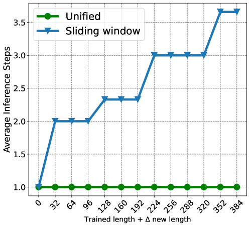
Figure 6: The comparison of average inference steps between our one-step unified inference and multi-step sliding window-based inference for zero-shot forecasting on new lengths.

References

- Arora et al. (2023) Arora, S., Narayan, A., Chen, M. F., Orr, L., Guha, N., Bhatia, K., Chami, I., and Re, C. Ask me anything: A simple strategy for prompting language models. In The Eleventh International Conference on Learning Representations, 2023. URL https://openreview.net/forum?id=bhUPJnS2g0X.
- Ashok et al. (2024) Ashok, A., Marcotte, É., Zantedeschi, V., Chapados, N., and Drouin, A. Tactis-2: Better, faster, simpler attentional copulas for multivariate time series. In International conference on learning representations, 2024.
- Bagnall et al. (2018) Bagnall, A., Dau, H. A., Lines, J., Flynn, M., Large, J., Bostrom, A., Southam, P., and Keogh, E. The uea multivariate time series classification archive, 2018. arXiv preprint arXiv:1811.00075, 2018.
- Bedda & Hammami (2010) Bedda, M. and Hammami, N. Spoken Arabic Digit. UCI Machine Learning Repository, 2010. DOI: https://doi.org/10.24432/C52C9Q.
- Birbaumer et al. (1999) Birbaumer, N., Ghanayim, N., Hinterberger, T., Iversen, I., Kotchoubey, B., Kübler, A., Perelmouter, J., Taub, E., and Flor, H. A spelling device for the paralysed. Nature, 398(6725):297–298, 1999.
- Bommasani et al. (2021) Bommasani, R., Hudson, D. A., Adeli, E., Altman, R., Arora, S., von Arx, S., Bernstein, M. S., Bohg, J., Bosselut, A., Brunskill, E., et al. On the opportunities and risks of foundation models. arXiv preprint arXiv:2108.07258, 2021.
- Brown et al. (2020) Brown, T., Mann, B., Ryder, N., Subbiah, M., Kaplan, J. D., Dhariwal, P., Neelakantan, A., Shyam, P., Sastry, G., Askell, A., et al. Language models are few-shot learners. Advances in neural information processing systems, 33:1877–1901, 2020.
- Cao et al. (2024) Cao, D., Jia, F., Arik, S. O., Pfister, T., Zheng, Y., Ye, W., and Liu, Y. TEMPO: Prompt-based generative pre-trained transformer for time series forecasting. In The Twelfth International Conference on Learning Representations, 2024. URL https://openreview.net/forum?id=YH5w12OUuU.
- (9) CDC. Illness. URL https://gis.cdc.gov/grasp/fluview/fluportaldashboard.html.
- Chang et al. (2023) Chang, C., Peng, W.-C., and Chen, T.-F. Llm4ts: Two-stage fine-tuning for time-series forecasting with pre-trained llms. arXiv preprint arXiv:2308.08469, 2023.
- Chen et al. (2023a) Chen, G., Yao, W., Song, X., Li, X., Rao, Y., and Zhang, K. PLOT: Prompt learning with optimal transport for vision-language models. In The Eleventh International Conference on Learning Representations, 2023a. URL https://openreview.net/forum?id=zqwryBoXYnh.
- Chen et al. (2023b) Chen, X., Deng, L., Zhao, Y., and Zheng, K. Adversarial autoencoder for unsupervised time series anomaly detection and interpretation. In Proceedings of the Sixteenth ACM International Conference on Web Search and Data Mining, pp. 267–275, 2023b.
- Chen et al. (2023c) Chen, Y., Deng, W., Fang, S., Li, F., Yang, N. T., Zhang, Y., Rasul, K., Zhe, S., Schneider, A., and Nevmyvaka, Y. Provably convergent schr” odinger bridge with applications to probabilistic time series imputation. In International Conference on Machine Learning, 2023c.
- Chen et al. (2023d) Chen, Y., Ren, K., Wang, Y., Fang, Y., Sun, W., and Li, D. Contiformer: Continuous-time transformer for irregular time series modeling. In Thirty-seventh Conference on Neural Information Processing Systems, 2023d. URL https://openreview.net/forum?id=YJDz4F2AZu.
- Chicaiza & Benalcázar (2021) Chicaiza, K. O. and Benalcázar, M. E. A brain-computer interface for controlling iot devices using eeg signals. In 2021 IEEE Fifth Ecuador Technical Chapters Meeting (ETCM), pp. 1–6. IEEE, 2021.
- Cuturi (2011) Cuturi, M. Fast global alignment kernels. In Proceedings of the 28th international conference on machine learning (ICML-11), pp. 929–936, 2011.
- Dau et al. (2018) Dau, H. A., Keogh, E., Kamgar, K., Yeh, C.-C. M., Zhu, Y., Gharghabi, S., Ratanamahatana, C. A., Yanping, Hu, B., Begum, N., Bagnall, A., Mueen, A., Batista, G., and Hexagon-ML. The ucr time series classification archive, October 2018. https://www.cs.ucr.edu/~eamonn/time_series_data_2018/.
- Ding et al. (2023) Ding, C., Sun, S., and Zhao, J. Mst-gat: A multimodal spatial–temporal graph attention network for time series anomaly detection. Information Fusion, 89:527–536, 2023.
- Dong et al. (2023) Dong, J., Wu, H., Zhang, H., Zhang, L., Wang, J., and Long, M. Simmtm: A simple pre-training framework for masked time-series modeling. arXiv preprint arXiv:2302.00861, 2023.
- Egede et al. (2020) Egede, J. O., Song, S., Olugbade, T. A., Wang, C., Amanda, C. D. C., Meng, H., Aung, M., Lane, N. D., Valstar, M., and Bianchi-Berthouze, N. Emopain challenge 2020: Multimodal pain evaluation from facial and bodily expressions. In 2020 15th IEEE International Conference on Automatic Face and Gesture Recognition (FG 2020), pp. 849–856. IEEE, 2020.
- Fraikin et al. (2024) Fraikin, A., Bennetot, A., and Allassonnière, S. T-rep: Representation learning for time series using time-embeddings. In The Twelfth International Conference on Learning Representations, 2024. URL https://openreview.net/forum?id=3y2TfP966N.
- Gao et al. (2019) Gao, S., Cheng, M.-M., Zhao, K., Zhang, X.-Y., Yang, M.-H., and Torr, P. Res2net: A new multi-scale backbone architecture. IEEE transactions on pattern analysis and machine intelligence, 43(2):652–662, 2019.
- Gao et al. (2023) Gao, S., Lin, Z., Xie, X., Zhou, P., Cheng, M.-M., and Yan, S. Editanything: Empowering unparalleled flexibility in image editing and generation. In Proceedings of the 31st ACM International Conference on Multimedia, pp. 9414–9416, 2023.
- Godahewa et al. (2021) Godahewa, R., Bergmeir, C., Webb, G. I., Hyndman, R. J., and Montero-Manso, P. Monash time series forecasting archive. In Neural Information Processing Systems Track on Datasets and Benchmarks, 2021.
- Goldberger et al. (2000a) Goldberger, A. L., Amaral, L. A., Glass, L., Hausdorff, J. M., Ivanov, P. C., Mark, R. G., Mietus, J. E., Moody, G. B., Peng, C.-K., and Stanley, H. E. Physiobank, physiotoolkit, and physionet: components of a new research resource for complex physiologic signals. circulation, 101(23):e215–e220, 2000a.
- Goldberger et al. (2000b) Goldberger, A. L., Amaral, L. A. N., Glass, L., Hausdorff, J. M., Ivanov, P. C., Mark, R. G., Mietus, J. E., Moody, G. B., Peng, C.-K., and Stanley, H. E. PhysioBank, PhysioToolkit, and PhysioNet: Components of a new research resource for complex physiologic signals. Circulation, 101(23):e215–e220, 2000b. Circulation Electronic Pages: http://circ.ahajournals.org/content/101/23/e215.full PMID:1085218; doi: 10.1161/01.CIR.101.23.e215.
- Gruver et al. (2023) Gruver, N., Finzi, M. A., Qiu, S., and Wilson, A. G. Large language models are zero-shot time series forecasters. In Thirty-seventh Conference on Neural Information Processing Systems, 2023.
- He et al. (2023) He, H., Queen, O., Koker, T., Cuevas, C., Tsiligkaridis, T., and Zitnik, M. Domain adaptation for time series under feature and label shifts. In Proceedings of the 40th International Conference on Machine Learning, ICML’23. JMLR.org, 2023.
- He et al. (2021) He, K., Chen, X., Xie, S., Li, Y., Dollár, P., and Girshick, R. Masked autoencoders are scalable vision learners. arXiv:2111.06377, 2021.
- Henson et al. (2011) Henson, R. N., Wakeman, D. G., Litvak, V., and Friston, K. J. A parametric empirical bayesian framework for the eeg/meg inverse problem: generative models for multi-subject and multi-modal integration. Frontiers in human neuroscience, 5:76, 2011.
- Huang et al. (2023) Huang, Q., Ren, H., Chen, P., Kržmanc, G., Zeng, D., Liang, P., and Leskovec, J. PRODIGY: Enabling in-context learning over graphs. In Thirty-seventh Conference on Neural Information Processing Systems, 2023. URL https://openreview.net/forum?id=pLwYhNNnoR.
- Hyndman (2015) Hyndman, R. expsmooth: Data sets from “forecasting with exponential smoothing”. R package version, 2, 2015.
- Hyndman & Athanasopoulos (2018) Hyndman, R. J. and Athanasopoulos, G. Forecasting: principles and practice. OTexts, 2018.
- Jin et al. (2023) Jin, M., Wang, S., Ma, L., Chu, Z., Zhang, J. Y., Shi, X., Chen, P.-Y., Liang, Y., Li, Y.-F., Pan, S., et al. Time-llm: Time series forecasting by reprogramming large language models. arXiv preprint arXiv:2310.01728, 2023.
- Kaltenborn et al. (2023) Kaltenborn, J., Lange, C. E. E., Ramesh, V., Brouillard, P., Gurwicz, Y., Nagda, C., Runge, J., Nowack, P., and Rolnick, D. Climateset: A large-scale climate model dataset for machine learning. In Thirty-seventh Conference on Neural Information Processing Systems Datasets and Benchmarks Track, 2023. URL https://openreview.net/forum?id=3z9YV29Ogn.
- Kim et al. (2023) Kim, S., Kim, H., Yun, E., Lee, H., Lee, J., and Lee, J. Probabilistic imputation for time-series classification with missing data. In International Conference on Machine Learning, pp. 16654–16667. PMLR, 2023.
- Kirillov et al. (2023) Kirillov, A., Mintun, E., Ravi, N., Mao, H., Rolland, C., Gustafson, L., Xiao, T., Whitehead, S., Berg, A. C., Lo, W.-Y., et al. Segment anything. arXiv preprint arXiv:2304.02643, 2023.
- Kudo et al. (1999) Kudo, M., Toyama, J., and Shimbo, M. Multidimensional curve classification using passing-through regions. Pattern Recognition Letters, 20(11-13):1103–1111, 1999.
- Lai et al. (2018) Lai, G., Chang, W.-C., Yang, Y., and Liu, H. Modeling long-and short-term temporal patterns with deep neural networks. In The 41st international ACM SIGIR conference on research & development in information retrieval, pp. 95–104, 2018.
- Lee et al. (2024) Lee, S., Park, T., and Lee, K. Learning to embed time series patches independently. In The Twelfth International Conference on Learning Representations, 2024. URL https://openreview.net/forum?id=WS7GuBDFa2.
- Lester et al. (2021) Lester, B., Al-Rfou, R., and Constant, N. The power of scale for parameter-efficient prompt tuning. In Moens, M.-F., Huang, X., Specia, L., and Yih, S. W.-t. (eds.), Proceedings of the 2021 Conference on Empirical Methods in Natural Language Processing, pp. 3045–3059, Online and Punta Cana, Dominican Republic, November 2021. Association for Computational Linguistics. doi: 10.18653/v1/2021.emnlp-main.243. URL https://aclanthology.org/2021.emnlp-main.243.
- Li & Jung (2023) Li, G. and Jung, J. J. Deep learning for anomaly detection in multivariate time series: Approaches, applications, and challenges. Information Fusion, 91:93–102, 2023.
- Li & Liang (2021) Li, X. L. and Liang, P. Prefix-tuning: Optimizing continuous prompts for generation. In Zong, C., Xia, F., Li, W., and Navigli, R. (eds.), Proceedings of the 59th Annual Meeting of the Association for Computational Linguistics and the 11th International Joint Conference on Natural Language Processing (Volume 1: Long Papers), pp. 4582–4597, Online, August 2021. Association for Computational Linguistics. doi: 10.18653/v1/2021.acl-long.353. URL https://aclanthology.org/2021.acl-long.353.
- Lines et al. (2011) Lines, J., Bagnall, A., Caiger-Smith, P., and Anderson, S. Classification of household devices by electricity usage profiles. In Intelligent Data Engineering and Automated Learning-IDEAL 2011: 12th International Conference, Norwich, UK, September 7-9, 2011. Proceedings 12, pp. 403–412. Springer, 2011.
- Liu et al. (2016) Liu, C., Springer, D., Li, Q., Moody, B., Juan, R. A., Chorro, F. J., Castells, F., Roig, J. M., Silva, I., Johnson, A. E., et al. An open access database for the evaluation of heart sound algorithms. Physiological measurement, 37(12):2181, 2016.
- Liu et al. (2023a) Liu, H., Li, C., Wu, Q., and Lee, Y. J. Visual instruction tuning. In Advances in neural information processing systems, 2023a.
- Liu et al. (2009) Liu, J., Zhong, L., Wickramasuriya, J., and Vasudevan, V. uwave: Accelerometer-based personalized gesture recognition and its applications. Pervasive and Mobile Computing, 5(6):657–675, 2009.
- Liu et al. (2021) Liu, S., Yu, H., Liao, C., Li, J., Lin, W., Liu, A. X., and Dustdar, S. Pyraformer: Low-complexity pyramidal attention for long-range time series modeling and forecasting. In International conference on learning representations, 2021.
- Liu et al. (2022a) Liu, X., Ji, K., Fu, Y., Tam, W., Du, Z., Yang, Z., and Tang, J. P-tuning: Prompt tuning can be comparable to fine-tuning across scales and tasks. In Proceedings of the 60th Annual Meeting of the Association for Computational Linguistics (Volume 2: Short Papers), pp. 61–68, 2022a.
- Liu et al. (2023b) Liu, Y., Li, C., Wang, J., and Long, M. Koopa: Learning non-stationary time series dynamics with koopman predictors. In Advances in neural information processing systems, 2023b.
- Liu et al. (2024) Liu, Y., Hu, T., Zhang, H., Wu, H., Wang, S., Ma, L., and Long, M. itransformer: Inverted transformers are effective for time series forecasting. In International Conference on Learning Representations, 2024.
- Liu et al. (2022b) Liu, Z., Mao, H., Wu, C.-Y., Feichtenhofer, C., Darrell, T., and Xie, S. A convnet for the 2020s. In Proceedings of the IEEE/CVF conference on computer vision and pattern recognition, pp. 11976–11986, 2022b.
- Liu et al. (2023c) Liu, Z., Ma, P., Chen, D., Pei, W., and Ma, Q. Scale-teaching: Robust multi-scale training for time series classification with noisy labels. In Thirty-seventh Conference on Neural Information Processing Systems, 2023c. URL https://openreview.net/forum?id=9D0fELXbrg.
- Lu et al. (2023) Lu, W., Wang, J., Sun, X., Chen, Y., and Xie, X. Out-of-distribution representation learning for time series classification. In The Eleventh International Conference on Learning Representations, 2023. URL https://openreview.net/forum?id=gUZWOE42l6Q.
- Luo et al. (2023) Luo, D., Cheng, W., Wang, Y., Xu, D., Ni, J., Yu, W., Zhang, X., Liu, Y., Chen, Y., Chen, H., et al. Time series contrastive learning with information-aware augmentations. In Proceedings of the AAAI Conference on Artificial Intelligence, volume 37, pp. 4534–4542, 2023.
- MacLeod & Gweon (2012) MacLeod, A. I. and Gweon, H. Optimal deseasonalization for monthly and daily geophysical time series. Journal of Environmental Statistics, 2012.
- Maggie et al. (2017) Maggie, Anava, O., Kuznetsov, V., and Cukierski, W. Web traffic time series forecasting, 2017. URL https://kaggle.com/competitions/web-traffic-time-series-forecasting.
- Malekzadeh et al. (2019) Malekzadeh, M., Clegg, R. G., Cavallaro, A., and Haddadi, H. Mobile sensor data anonymization. In Proceedings of the international conference on internet of things design and implementation, pp. 49–58, 2019.
- Middlehurst et al. (2023) Middlehurst, M., Schäfer, P., and Bagnall, A. Bake off redux: a review and experimental evaluation of recent time series classification algorithms. arXiv preprint arXiv:2304.13029, 2023.
- Naiman et al. (2024) Naiman, I., Erichson, N. B., Ren, P., Mahoney, M. W., and Azencot, O. Generative modeling of regular and irregular time series data via koopman vaes. International conference on learning representations, 2024.
- Nate Gruver & Wilson (2023) Nate Gruver, Marc Finzi, S. Q. and Wilson, A. G. Large Language Models Are Zero Shot Time Series Forecasters. In Advances in Neural Information Processing Systems, 2023.
- Nie et al. (2023) Nie, Y., H. Nguyen, N., Sinthong, P., and Kalagnanam, J. A time series is worth 64 words: Long-term forecasting with transformers. In International Conference on Learning Representations, 2023.
- (63) NREL. Solar power data for integration studies. URL https://www.nrel.gov/grid/solar-power-data.html.
- Olszewski (2001) Olszewski, R. T. Generalized feature extraction for structural pattern recognition in time-series data. Carnegie Mellon University, 2001.
- (65) PeMS. Traffic. URL http://pems.dot.ca.gov/.
- Pourpanah et al. (2022) Pourpanah, F., Abdar, M., Luo, Y., Zhou, X., Wang, R., Lim, C. P., Wang, X.-Z., and Wu, Q. J. A review of generalized zero-shot learning methods. IEEE transactions on pattern analysis and machine intelligence, 2022.
- Queen et al. (2023) Queen, O., Hartvigsen, T., Koker, T., He, H., Tsiligkaridis, T., and Zitnik, M. Encoding time-series explanations through self-supervised model behavior consistency. In Thirty-seventh Conference on Neural Information Processing Systems, 2023. URL https://openreview.net/forum?id=yEfmhgwslQ.
- Radford et al. (2019) Radford, A., Wu, J., Child, R., Luan, D., Amodei, D., and Sutskever, I. Language models are unsupervised multitask learners. 2019.
- Radford et al. (2021) Radford, A., Kim, J. W., Hallacy, C., Ramesh, A., Goh, G., Agarwal, S., Sastry, G., Askell, A., Mishkin, P., Clark, J., et al. Learning transferable visual models from natural language supervision. In International conference on machine learning, pp. 8748–8763. PMLR, 2021.
- Rasul et al. (2023) Rasul, K., Ashok, A., Williams, A. R., Khorasani, A., Adamopoulos, G., Bhagwatkar, R., Biloš, M., Ghonia, H., Hassen, N. V., Schneider, A., et al. Lag-llama: Towards foundation models for time series forecasting. arXiv preprint arXiv:2310.08278, 2023.
- Rebbapragada et al. (2009) Rebbapragada, U., Protopapas, P., Brodley, C. E., and Alcock, C. Finding anomalous periodic time series: An application to catalogs of periodic variable stars. Machine learning, 74:281–313, 2009.
- Rombach et al. (2022) Rombach, R., Blattmann, A., Lorenz, D., Esser, P., and Ommer, B. High-resolution image synthesis with latent diffusion models. In Proceedings of the IEEE/CVF conference on computer vision and pattern recognition, pp. 10684–10695, 2022.
- Roverso (2002) Roverso, D. Plant diagnostics by transient classification: The aladdin approach. International Journal of Intelligent Systems, 17(8):767–790, 2002.
- Shokoohi-Yekta et al. (2017) Shokoohi-Yekta, M., Hu, B., Jin, H., Wang, J., and Keogh, E. Generalizing dtw to the multi-dimensional case requires an adaptive approach. Data mining and knowledge discovery, 31:1–31, 2017.
- Silva et al. (2013) Silva, I., Behar, J., Sameni, R., Zhu, T., Oster, J., Clifford, G. D., and Moody, G. B. Noninvasive fetal ecg: the physionet/computing in cardiology challenge 2013. In Computing in cardiology 2013, pp. 149–152. IEEE, 2013.
- Taieb et al. (2012) Taieb, S. B., Bontempi, G., Atiya, A. F., and Sorjamaa, A. A review and comparison of strategies for multi-step ahead time series forecasting based on the nn5 forecasting competition. Expert systems with applications, 39(8):7067–7083, 2012.
- Touvron et al. (2023) Touvron, H., Lavril, T., Izacard, G., Martinet, X., Lachaux, M.-A., Lacroix, T., Rozière, B., Goyal, N., Hambro, E., Azhar, F., et al. Llama: Open and efficient foundation language models. arXiv preprint arXiv:2302.13971, 2023.
- Trindade (2015) Trindade, A. ElectricityLoadDiagrams20112014. UCI Machine Learning Repository, 2015. DOI: https://doi.org/10.24432/C58C86.
- Trirat et al. (2024) Trirat, P., Shin, Y., Kang, J., Nam, Y., Na, J., Bae, M., Kim, J., Kim, B., and Lee, J.-G. Universal time-series representation learning: A survey. arXiv preprint arXiv:2401.03717, 2024.
- Villar et al. (2016) Villar, J. R., Vergara, P., Menéndez, M., de la Cal, E., González, V. M., and Sedano, J. Generalized models for the classification of abnormal movements in daily life and its applicability to epilepsy convulsion recognition. International journal of neural systems, 26(06):1650037, 2016.
- Wang et al. (2022) Wang, H., Peng, J., Huang, F., Wang, J., Chen, J., and Xiao, Y. Micn: Multi-scale local and global context modeling for long-term series forecasting. In The Eleventh International Conference on Learning Representations, 2022.
- Wang et al. (2020) Wang, Y., Yao, Q., Kwok, J. T., and Ni, L. M. Generalizing from a few examples: A survey on few-shot learning. ACM computing surveys (csur), 53(3):1–34, 2020.
- Wang et al. (2023) Wang, Y., Han, Y., Wang, H., and Zhang, X. Contrast everything: A hierarchical contrastive framework for medical time-series. In Thirty-seventh Conference on Neural Information Processing Systems, 2023. URL https://openreview.net/forum?id=sOQBHlCmzp.
- (84) Wetterstation. Weather. URL https://www.bgc-jena.mpg.de/wetter/.
- Wu et al. (2021) Wu, H., Xu, J., Wang, J., and Long, M. Autoformer: Decomposition transformers with auto-correlation for long-term series forecasting. Advances in Neural Information Processing Systems, 34:22419–22430, 2021.
- Wu et al. (2023) Wu, H., Hu, T., Liu, Y., Zhou, H., Wang, J., and Long, M. Timesnet: Temporal 2d-variation modeling for general time series analysis. In International Conference on Learning Representations, 2023.
- Xiao et al. (2022) Xiao, Q., Wu, B., Zhang, Y., Liu, S., Pechenizkiy, M., Mocanu, E., and Mocanu, D. C. Dynamic sparse network for time series classification: Learning what to “see”. In Oh, A. H., Agarwal, A., Belgrave, D., and Cho, K. (eds.), Advances in Neural Information Processing Systems, 2022. URL https://openreview.net/forum?id=ZxOO5jfqSYw.
- Xu et al. (2024) Xu, M. A., Moreno, A., Wei, H., Marlin, B. M., and Rehg, J. M. Retrieval-based reconstruction for time-series contrastive learning. In The Twelfth International Conference on Learning Representations, 2024. URL https://openreview.net/forum?id=3zQo5oUvia.
- Zeng et al. (2023) Zeng, A., Chen, M., Zhang, L., and Xu, Q. Are transformers effective for time series forecasting? In Proceedings of the AAAI conference on artificial intelligence, volume 37, pp. 11121–11128, 2023.
- Zerveas et al. (2021) Zerveas, G., Jayaraman, S., Patel, D., Bhamidipaty, A., and Eickhoff, C. A transformer-based framework for multivariate time series representation learning. In Proceedings of the 27th ACM SIGKDD Conference on Knowledge Discovery & Data Mining, KDD ’21, pp. 2114–2124, New York, NY, USA, 2021. Association for Computing Machinery. ISBN 9781450383325. doi: 10.1145/3447548.3467401.
- Zhang et al. (2022a) Zhang, H., Zhang, P., Hu, X., Chen, Y.-C., Li, L. H., Dai, X., Wang, L., Yuan, L., Hwang, J.-N., and Gao, J. GLIPv2: Unifying localization and vision-language understanding. In Oh, A. H., Agarwal, A., Belgrave, D., and Cho, K. (eds.), Advances in Neural Information Processing Systems, 2022a. URL https://openreview.net/forum?id=wiBEFdAvl8L.
- Zhang et al. (2022b) Zhang, X., Zeman, M., Tsiligkaridis, T., and Zitnik, M. Graph-guided network for irregularly sampled multivariate time series. In International Conference on Learning Representations, ICLR, 2022b.
- Zhang et al. (2022c) Zhang, X., Zhao, Z., Tsiligkaridis, T., and Zitnik, M. Self-supervised contrastive pre-training for time series via time-frequency consistency. Advances in Neural Information Processing Systems, 2022c.
- Zhang & Yang (2021) Zhang, Y. and Yang, Q. A survey on multi-task learning. IEEE Transactions on Knowledge and Data Engineering, 34(12):5586–5609, 2021.
- Zhang et al. (2023) Zhang, Y., Gong, K., Zhang, K., Li, H., Qiao, Y., Ouyang, W., and Yue, X. Meta-transformer: A unified framework for multimodal learning. arXiv preprint arXiv:2307.10802, 2023.
- Zhou et al. (2021) Zhou, H., Zhang, S., Peng, J., Zhang, S., Li, J., Xiong, H., and Zhang, W. Informer: Beyond efficient transformer for long sequence time-series forecasting. In Proceedings of the AAAI conference on artificial intelligence, volume 35, pp. 11106–11115, 2021.
- Zhou et al. (2022) Zhou, T., Ma, Z., Wen, Q., Wang, X., Sun, L., and Jin, R. Fedformer: Frequency enhanced decomposed transformer for long-term series forecasting. In International Conference on Machine Learning, pp. 27268–27286. PMLR, 2022.
- Zhou et al. (2023) Zhou, T., Niu, P., Wang, X., Sun, L., and Jin, R. One fits all: Power general time series analysis by pretrained LM. In Thirty-seventh Conference on Neural Information Processing Systems, 2023. URL https://openreview.net/forum?id=gMS6FVZvmF.
- Zhu et al. (2022) Zhu, J., Zhu, X., Wang, W., Wang, X., Li, H., Wang, X., and Dai, J. Uni-Perceiver-MoE: Learning sparse generalist models with conditional moes. Advances in Neural Information Processing Systems, 35:2664–2678, 2022.