A moment tensor potential for lattice thermal conductivity
calculations of $\alpha$ and $\beta$ phases of Ga₂O₃

Abstract

Calculations of heat transport in crystalline materials have recently become mainstream, thanks to machine-learned interatomic potentials that allow for significant computational cost reductions while maintaining the accuracy of first-principles calculations. Moment tensor potentials (MTP) are among the most efficient and accurate models in this regard. In this study, we demonstrate the application of MTP to the calculation of the lattice thermal conductivity of $\alpha$ and $\beta$-Ga₂O₃. Although MTP is commonly employed for lattice thermal conductivity calculations, the advantages of applying the active learning methodology for potential generation is often overlooked. Here, we emphasize its importance and illustrate how it enables the generation of a robust and accurate interatomic potential while maintaining a moderate-sized training dataset.

I Introduction

Lattice thermal conductivity (LTC) is an essential quantity for a wide range of technological applications, including thermal management of microelectronic devices Moore and Shi (2014), thermoelectrics Tan, Zhao, and Kanatzidis (2016), and thermal barrier coating materials Clarke and Phillpot (2005). Accurate experimental measurement of LTC is challenging and reproducibility between different experimental groups is often not guaranteed Wei et al. (2016). Consequently, despite the technological need, reliable LTC data are known for only a small number of materials. At the same time, the theoretical formulation of heat transport constitutes a mature research field Peierls (1929); Maradudin and Fein (1962). From a practical perspective, calculations of the temperature-dependent LTC are usually based on a perturbative approach, the Green-Kubo approach (GK) Kubo, Yokota, and Nakajima (1957); Meng et al. (2019), or non-equilibrium molecular dynamics simulations (NEMD). In a perturbative approach Broido et al. (2007), calculations are typically performed within the framework of first-principles (or ab initio) density-functional theory (DFT). In practice, perturbative approaches require calculation of the so-called interatomic force constants (IFCs), which is time-consuming, especially for structures with large unit cells and low symmetry. This is because the number of structures with displaced atoms needed to construct third-order IFCs grows enormously fast with reduction of the crystalline symmetry Togo et al. (2023).

Materials with large anharmonicities are not rare and sometimes accurate evaluation of lattice dynamics of such materials require to consider the inclusion of all orders of anharmonicity Knoop et al. (2020). Already the influence of four-phonon scattering processes on LTC of solids can have huge impact Feng and Ruan (2016); Feng, Lindsay, and Ruan (2017). For example, in the case of boron arsenide (BAs) and graphene, better agreement between theory and experiment can only be achieved when four-phonon scattering is taken into account Kang et al. (2018); Tian et al. (2018); Li et al. (2018); Wang et al. (2023). In principle, lattice dynamics anharmonicity can be fully and accurately taken into account in ab initio molecular dynamics (AIMD) simulations. Hence, both the GK and NEMD approaches utilize AIMD and allow for a more accurate computation of LTC, as all orders of anharmonicity are taken into account. However, these methods are computationally expensive. The Green-Kubo formula relates instantaneous fluctuations of heat current in terms of the autocorrelation function. While the formulation of GK was done long ago, first-principles calculations of LTC using this approach have only recently appeared Carbogno, Ramprasad, and Scheffler (2017). The evaluation of LTC using the Green-Kubo approach coupled with first-principles calculations is rare, albeit its profound influence on the understanding of the heat transport Knoop et al. (2023). However, converging LTC values is a challenging task, as AIMD simulations are severely limited by system size (a few hundred atoms) and timescales (tens of picoseconds). Thus, GK and NEMD approaches are limited in applicability when coupled with first-principles calculations.

Challenges associated with the experimental measurements and theoretical calculations of the LTC lead to the lack of a systematic understanding of the LTC beyond semi-empirical and phenomenological trends in a very limited number of simple materials Morelli and Slack (2006). From the computational perspective, speed up can be obtained by performing molecular dynamics (MD) simulations using empirical potentials, which enables one to efficiently predict properties of both bulk materials and nanostructures, over a wider range of system sizes (up to hundreds of nanometers) Kadau, Germann, and Lomdahl (2006) and timescales (up to tens of nanoseconds) Böckmann and Grubmüller (2002). However, the prediction accuracy will be highly dependent on the fidelity of the potentials. On the other hand, machine learning methods (ML) can be used to predict LTC values. In some cases ML models are trained in a supervised manner Jaafreh, Kang, and Hamad (2021); Purcell et al. (2023); Luo et al. (2023) and in some cases machine-learned interatomic potentials (MLIPs) Deringer, Caro, and Csányi (2019); Bartók et al. (2017) are used to either compute IFCs Mortazavi et al. (2020, 2021); Ouyang et al. (2022) or to directly perform MD simulations Mortazavi et al. (2020); Arabha et al. (2021); Verdi et al. (2021); Korotaev et al. (2019). Among different MLIP models the moment tensor potential (MTP) Shapeev (2016) showed substantial accuracy keeping the required training data at a minimum size Zuo et al. (2020), especially once the active learning (sometimes terms active sampling or learning on-the-fly are used) methodology is used Podryabinkin and Shapeev (2017). Despite wide application of different MLIPs, the training process is still frequently done without the active learning scheme. In this case the potential is usually trained on some AIMD trajectories and its ability to extrapolate is typically limited only to this training set. Recently, we demonstrated that low root-mean-squared errors on the training and test sets do not guarantee the robustness of a potential Nikita et al. (2024), which we define as an ability to run long MD simulations without failure. This outcome underscores that while low energy and force errors are achieved, applicability and accuracy of such MLIP should be taken with a portion of scepticism, even if the lattice dynamics calculations are performed under the same thermodynamic conditions as those employed during the training data generation.

In this work, we demonstrate how to generate a robust and accurate MTP using the active learning approach. Its employment not only ensures the applicability of MTP for lattice dynamics simulations, but also substantially reduces the number of the required DFT calculations. As a benchmark systems, we used $\alpha$- and $\beta$-Ga₂O₃. Both $\alpha$ and $\beta$ phases of Ga₂O₃ are wide-bandgap semiconductors of significant technological importance Shan et al. (2005); Pearton et al. (2018); Higashiwaki et al. (2017); Singh Pratiyush et al. (2017); Fleischer and Meixner (1992); Zhou et al. (2017); Cheng et al. (2020). Consequently, these materials are well-investigated both experimentally Guo et al. (2015); Galazka et al. (2014); Handwerg et al. (2015); Jiang et al. (2018) and theoretically Santia, Tandon, and Albrecht (2015); Yan and Kumar (2018). Moreover, given the large conventional cell of $\beta$-Ga₂O₃ containing 20 atoms, the first-principles calculations are highly time-consuming especially when extensive convergence tasks need to be performed, which highlights the role of MLIPs usage as would be demonstrated here.

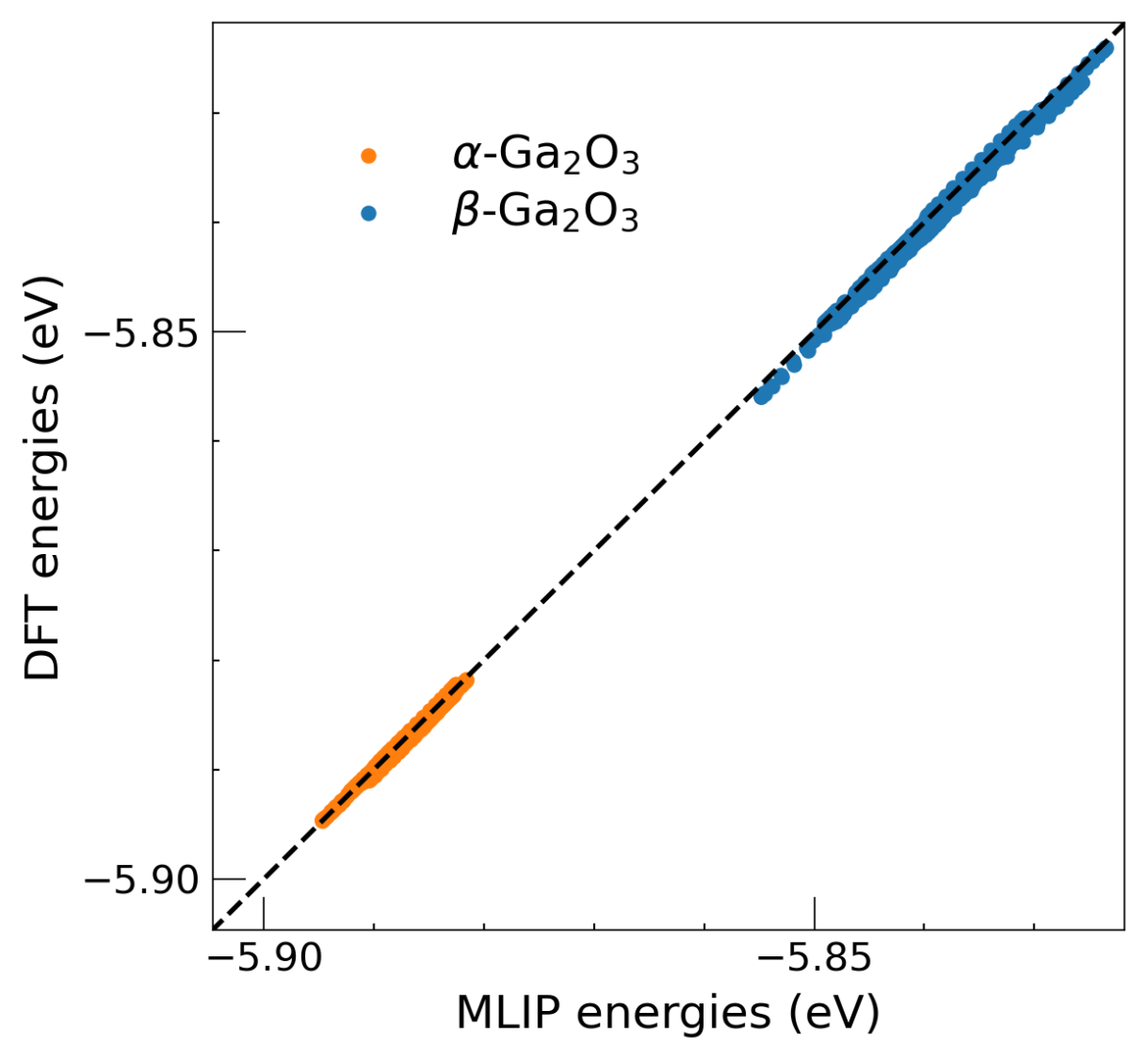
(a)

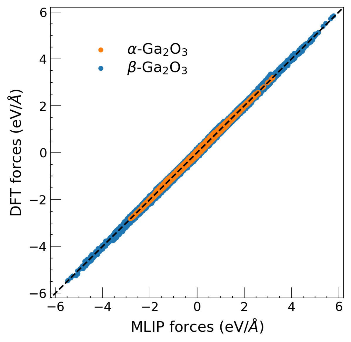
(b)

Figure 1: Comparison between DFT- and MTP-calculated (a) energies and (b) forces for both $\alpha$- and $\beta$-Ga₂O₃ structures. Straight black line represents a perfect linear dependence.

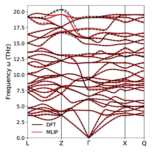
(a)

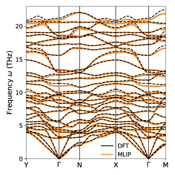
(b)

Figure 2: Phonon dispersion relation of (a) $\alpha$- and (b) $\beta$-Ga₂O₃ along selected high symmetry Brillouin zone path. Calculations are done using DFT and MTP.

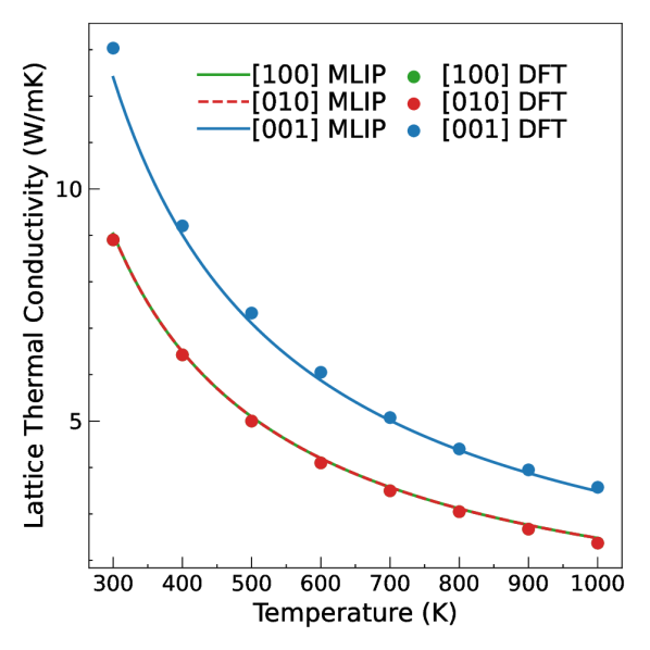
(a)

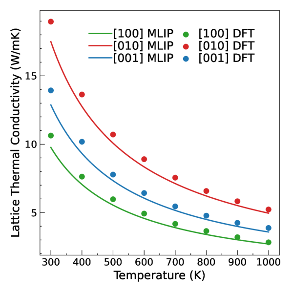
(b)

Figure 3: Temperature dependence of the LTC of (a) $\alpha$-Ga₂O₃ and (b) $\beta$-Ga₂O₃ for three different directions. LTC calculations with MLIP (moment tensor potential in our case) are compared to the recent calculations, which were done in the DFT framework Yang et al. (2023).

II Methodology

II.1 Construction of a Moment Tensor Potential

The potential energy of an atomic system as described by the MTP interatomic potential is defined as a sum of the energies of atomic environments of the individual atoms:

$$E_{\text{MTP}}=\sum_{i=1}^{N}V(n_{i}),$$

where the index $i$ label $N$ atoms of the system, and $n_{i}$ describes the local atomic neighborhood around atom i within a certain cutoff radius $R_{\text{cut}}$, i.e., a many-body descriptor can comprise the information of all neighbors of a centered atom up to a given cutoff radius. The function $V$ is the moment tensor potential:

$$V(n_{i})=\sum_{\alpha}\xi_{\alpha}B_{\alpha}(n_{i}),$$

where $\xi_{\alpha}$ are the fitting parameters and $B_{\alpha}(n_{i})$ are the basis functions that will be defined below. Moment tensors descriptors are used as representations of atomic environments and defined as:

$$M_{\mu,\nu}\left({n}_{i}\right)=\sum_{j}f_{\mu}\left(\left|r_{ij}\right|,z_{i},z_{j}\right)\underbrace{r_{ij}\otimes\ldots\otimes r_{ij}}_{\nu\text{ times }},$$

where the index $j$ goes through all the neighbors of atom $i$. The symbol “$\otimes$” stands for the outer product of vectors, thus ${r}_{ij}\otimes\cdots\otimes{r}_{ij}$ is the tensor of rank $\nu$ encoding the angular part which itself resembles moments of inertia. The function $f_{\mu}$ represents the radial component of the moment tensor:

$$f_{\mu}\left(\left|r_{ij}\right|,z_{i},z_{j}\right)=\sum_{k}c_{\mu,z_{i},z_{j}}^{(k)}Q^{(k)}(r),$$

where $z_{i}$ and $z_{j}$ denote the atomic species of atoms $i$ and $j$, respectively, $r_{ij}$ describes the positioning of atom $j$ relative to atom $i$, $c_{\mu,z_{i},z_{j}}^{(k)}$ are the fitting parameters and

$$Q^{(k)}(r):=T_{k}(r)\left(R_{\text{cut }}-r\right)^{2}$$

are the radial functions consisting of the Chebyshev polynomials $T_{k}(r)$ on the interval $[R_{\text{min}},R_{\text{cut}}]$ with the term ($R_{\text{cut}}-r)^{2}$ that is introduced to ensure a smooth cut-off to zero. The descriptors $M_{\mu,\nu}$ taking $\nu$ equal to $0,1,2,\ldots$ are tensors of different ranks that allow to define basis functions as all possible contractions of these tensors to a scalar, for instance:

$$B_{0}\left({n}_{i}\right)=M_{0,0}\left({n}_{i}\right)$$

$$B_{1}\left({n}_{i}\right)=M_{0,1}\left({n}_{i}\right)\cdot M_{0,1}\left({n}_{i}\right),$$

$$B_{2}\left({n}_{i}\right)=M_{0,0}\left({n}_{i}\right)\left(M_{0,2}\left({n}_{i}\right):M_{0,2}\left({n}_{i}\right)\right).$$

Therefore the level of $M_{\mu,\nu}$ is defined by ${\rm lev}M_{\mu,\nu}$ = 2$\mu$ + $\nu$ and if $B_{\alpha}$ is obtained from $M_{\mu_{1},\nu_{1}}$ , $M_{\mu_{2},\nu_{2}}$ , $\dots$, then ${\rm lev}B_{\alpha}$ = $(2\mu_{1}+\nu_{1})$ + $(2\mu_{2}+\nu_{2})$ + $\dots$ . By including all basis functions such that ${\rm lev}B_{\alpha}<d$ we obtain the moment tensor potential of level $d$ which we denote as MTP_d.

As fundamental symmetry requirements, all descriptors for atomic environment have to be invariant to translation, rotation, and permutation with respect to the atomic indexing. Particularly for structurally intricate Ga₂O₃ polymorphs, the incorporation of many-body interactions is crucial to ensuring the accuracy of the derived potentials. The MTP framework satisfies all aforementioned conditions Shapeev (2016). Importantly, the MTP framework satisfies all aforementioned conditions Shapeev (2016). MTP methodology and tools to utilize it are implemented in the MLIP-2 package Novikov et al. (2020), which we used in this work.

II.2 Generation of a Training Set

We conducted aiMD simulations to collect the reference data (potential energy, atomic forces, atomic coordinates)) for MTP training. aiMD simulations are conducted within the DFT framework, employing VASP (Vienna ab initio simulations package) Kresse and Furthmüller (1996) with the projector augmented wave method Kresse and Joubert (1999). The Perdew-Burke-Ernzerhof generalized gradient approximation (PBE-GGA) Perdew, Burke, and Ernzerhof (1996) was employed for the exchange–correlation functional. We used a plane wave basis set cut-off of 550 eV, and a Gaussian smearing of 0.1 eV width. The halting criterion for electronic density convergence during self-consistent field calculations is set to 10^-7 eV.

The corundum structure of $\alpha$-Ga₂O₃ has a space group $R\bar{3}c$, while $\beta$-Ga₂O₃ has a monoclinic structure with the space group $C2/m$. The optimized structural parameters obtained in our calculations are shown in the Tab. 1. These structural parameters are in a good agreement with the experimental data Åhman, Svensson, and Albertsson (1996). All lattice dynamics calculations in this work were performed with these structures. The conventional cells was sampled using 6$\times$6$\times$2 k-point grids for $\alpha$-Ga₂O₃ and for $\beta$-Ga₂O₃, respectively. In case of the lattice dynamics calculations, we used 2$\times$2$\times$1 diagonal transformation matrix to generate a supercell with 120 atoms from the conventional $\alpha$-Ga₂O₃ cell. In the case of $\beta$-Ga₂O₃ we generated a supercell with 160 atoms expanding the conventional cell using 6$\times$6$\times$2 diagonal transformation matrix. For the calculations with supercells, the k-point grids were adjusted to keep the k-points’ mesh density as in the calculations with the unit cells, this leads to the utilization of only one $\Gamma$-point in both cases.

Table 1: PBE-optimized unit cell vectors and angles of the $\alpha$- and $\beta$-Ga₂O₃ phases.

Phase	a, (Å)	b, (Å)	c, (Å)	$\alpha$	$\beta$	$\gamma$
$\alpha$-Ga2O3	5.065	5.065	13.64	90∘	90∘	120∘
$\beta$-Ga2O3	12.469∘	3.087	5.882	90∘	103.673∘	90∘

Typically, two main approaches are employed to train a reliable MLIP capable of accurately representing a wide spectrum of local atomic environments. The first one involves the inclusion of various systems, necessitating extensive AIMD simulations. By incorporating a diverse range of systems, the MLIP can effectively learn to capture the nuances of different atomic environments. The second approach is called active learning and it involves the selective addition of data points to the training set, focusing on structures where the MLIP extrapolates significantly. These are instances where the MLIP’s predictions for energies and forces exhibit high uncertainty. By strategically choosing a minimal yet diverse set of training data in the feature space, this active learning strategy enables effective fitting of the potential and helps overcome extrapolation challenges. In this study, we generate a small dataset to pretrain the MLIP. Subsequently, we employ an active learning strategy to iteratively expand this dataset, ensuring the MLIP’s robustness and accuracy for lattice dynamics calculations. We advocate for the consistent use of the active learning methodology due to its efficacy in enhancing the MLIP’s performance and thus, revisit it briefly here.

Various active learning schemes are employed in the development of machine learning potentials Zhang et al. (2019); Sivaraman et al. (2020). In our study, we utilized the D-optimality-based active learning procedure developed in Podryabinkin and Shapeev (2017) and available in the MLIP-2 package. The initial training set was generated in aiMD simulations with isothermal-isobaric (NPT) ensemble using the Nosé-Hoover thermostat Nosé (1984). The initial dataset was generated at T=700 K for $\alpha$ phase and at T=1800 K for $\beta$ phase, respectively. Each AIMD trajectory was simulated for 2 ps with a 1 fs time step. Initial structures for AIMD were prethermalized following the algorithm established in West and Estreicher (2006), which allows to equilibrate simulations at finite temperatures faster. The first picosecond of each AIMD simulation was discarded, and the second picosecond was subsampled with the 5 fs time intervals, resulting in a set of 200 snapshots for each structure. These samples were employed to train an initial MTP of level 12.

Within the active learning algorithm, we initiate MD calculations in LAMMPS (Large-scale Atomic/Molecular Massively Parallel Simulator) Thompson et al. (2022) using a pretrained MTP as the model for interatomic interactions in the NVE ensemble. At each step of the MD simulations, the algorithm assesses the extrapolation grade $\gamma$ of the atomic configuration. The D-optimality criterion guides the decision to include a configuration in the training set, based solely on atomic coordinates. This unique feature, coupled with the linear form of the potential, allows MTP to learn effectively on-the-fly. Configurations with $\gamma>2$ are added to the preselected set. When $\gamma$ exceeds 10, the MD simulation halts, and all sufficiently different configurations from the preselected set are incorporated into the training, followed by the refitting of the potential. This procedure repeats until MD simulations can run without failure for 30 ps. In our case, MTP achieved robustness with a training set comprising 439 samples in the case of $\alpha$-Ga₂O₃ and 403 samples in the case of $\beta$-Ga₂O₃. This amount of samples is two times to an order of magnitude smaller than for other machine-learning potentials Li et al. (2018); Liu et al. (2020). The potential trained in this manner demonstrated the ability to robustly conduct MD simulations for 100 ps, showcasing the effectiveness of the active learning procedure in terms of reducing the necessary DFT data for training and enhancing potential robustness. The training set generated during the active learning procedure was then used to train MTP with level 16.

The fitting accuracy of obtained potential can be verified by the agreement between MTP predictions and the benchmark AIMD results. We compare the MTP-predicted energies and forces for a separate testing dataset formed by running AIMD for 1 ps with time steps of 1 fs (this dataset contains 1000 snapshots) at T=700 K for $\alpha$ and T=1800 K for $\beta$ phases, respectively. It is found that our MTP can provide the root mean square errors of 0.2 and 0.6 meV/atom for the potential energy of $\alpha$ and $\beta$ phases. The RMSEs for the atomic forces are 22 meV/Å and 46 meV/Å for $\alpha$ and $\beta$ phases, respectively. Therefore, MTP can accurately reproduce ab initio energies and forces as also visually demonstrated in Fig. 1(a, b).

III Results and Discussions

Harmonic or second-order force constants can be used to evaluate the accuracy of MTP compared to to DFT. We thus calculate the phonon dispersion relation along selected high symmetry paths, using the supercell approach and the finite displacement method Parlinski, Li, and Kawazoe (1997), as implemented in the Phonopy package Togo and Tanaka (2015). Figs. 2 (a, b) show calculated phonon dispersion relations obtained using MTP and DFT for both polymorphs of Ga₂O₃, respectively. We note good agreement between both methods, which validates an ability of MTP to describe the lattice dynamics in the harmonic approximation. Notably, existing empirical potentials frequently fail to capture that Blanco et al. (2005); Ma, Zhang, and Zhang (2020). The most observable differences in the phonon spectrum might be seen for high-frequency optical phonon modes (especially at the Z-point in Fig. 2 (a)). This is a usual problem frequently arising in the harmonic constants simulations with MLIPs Mortazavi et al. (2020); Li et al. (2018). From our experience, it is possible to improve the accuracy of optical phonon modes evaluation by performing simulations at high temperatures for a set of compressed and expanded structures Mortazavi et al. (2021); Liu et al. (2020). In this work we skipped this procedure, since obtaining precise values of LTC is not the primarily goal of this work. Considering the low symmetry and high anisotropy of $\beta$-Ga₂O₃, it is reasonable to see that the phonon dispersion profile is much more complex than that of many other wide-bandgap materials, such as GaN and ZnO Wu et al. (2016). Due to the versatility stemming from the relatively high complexity of the MTP functional form, harmonic force constants can be accurately reproduced — this precision is crucial as it serves as a fundamental prerequisite for conducting calculations of the LTC.

We next proceed towards LTC calculations, which was evaluated by solving Boltzmann transport equation for phonons in the relaxation time approximation as implemented in the Phono3py package Togo, Chaput, and Tanaka (2015); Mizokami, Togo, and Tanaka (2018); Togo et al. (2023). Here we should mention that in the case of $\alpha$-Ga₂O₃ one has to compute forces acting on atoms in 4087 supercells (with 120 atoms) and in the case of $\beta$-Ga₂O₃ in 15225 supercells (with 160 atoms). Albeit the crystalline symmetry is taken into account to reduce the number of calculations, these numbers are tangible even for calculations on modern high-performance clusters. Performing these calculations with MTP as a model for interatomic interactions takes minutes on a personal workstation.

Figs. 3 (a, b) present temperature dependence of the LTC for $\alpha$ and $\beta$ polymorphs. Values of LTC obtained using MTP are in a good agreement with most recent DFT calculations Yang et al. (2023), for example, at 300 K LTC values along [100] are identical up to the second decimal. Since $\beta$-Ga₂O₃ has a monoclinic structure, its [001] direction does not align with the $z$-axis. Therefore, we calculated its LTC in the [001] direction as was done in previous works Li et al. (2018); Yang et al. (2023): $\kappa_{[001]}$=$\cos^{2}{\beta}\kappa_{xx}+\sin{2\beta}\kappa_{xz}+\sin^{2}{\beta}\kappa_{zz}$. Notably, MTP caught the anisotropy in LTC values along different directions in both $\alpha$- and $\beta$-Ga₂O₃, which further validates its accuracy. The difference between our results and previous theoretical calculations Yang et al. (2023) is within 5-10%, which might be easily associated with different structural parameters or calculations set up between studies. Taken into account tremendous reduction of simulation time, we do not consider this as a significant problem.

IV Conclusion

In summary, we developed MTPs for atomistic simulations of $\alpha$ and $\beta$-Ga₂O₃. Our potentials exhibit good accuracy in reproducing the ab initio PES, attaining a total energy accuracy below 1 meV/atom and force accuracy below 50 meV/Å for both polymorphs. We then compared phonon dispersion and LTC values calculated using MTP with the results of DFT, and obtained good agreement, which highlights the applicability of MTP in calculating the lattice dynamics and heat transport of solids. The proper choice of training data to generate an accurate potential using as little data as possible is governed by the utilization of the active learning methodology. Although the possibility of its usage is frequently ignored, the active learning scheme plays a crucial role in enhancing the robustness of the machine-learned interatomic potentials, as demonstrated here.

Data Availability Statement

The data that support the findings of this study are available from the corresponding author upon reasonable request.

References

- Moore and Shi (2014) A. L. Moore and L. Shi, “Emerging challenges and materials for thermal management of electronics,” Materials Today 17, 163–174 (2014).
- Tan, Zhao, and Kanatzidis (2016) G. Tan, L.-D. Zhao, and M. G. Kanatzidis, “Rationally designing high-performance bulk thermoelectric materials,” Chemical Reviews 116, 12123–12149 (2016), pMID: 27580481.
- Clarke and Phillpot (2005) D. R. Clarke and S. R. Phillpot, “Thermal barrier coating materials,” Materials Today 8, 22–29 (2005).
- Wei et al. (2016) P.-C. Wei, S. Bhattacharya, J. He, S. Neeleshwar, R. Podila, Y. Y. Chen, and A. M. Rao, “The intrinsic thermal conductivity of snse,” Nature 539, E1–E2 (2016).
- Peierls (1929) R. Peierls, “Zur kinetischen theorie der wärmeleitung in kristallen,” Annalen der Physik 395, 1055–1101 (1929).
- Maradudin and Fein (1962) A. Maradudin and A. Fein, “Scattering of neutrons by an anharmonic crystal,” Physical Review 128, 2589 (1962).
- Kubo, Yokota, and Nakajima (1957) R. Kubo, M. Yokota, and S. Nakajima, “Statistical-mechanical theory of irreversible processes. ii. response to thermal disturbance,” Journal of the Physical Society of Japan 12, 1203–1211 (1957).
- Meng et al. (2019) H. Meng, X. Yu, H. Feng, Z. Xue, and N. Yang, “Superior thermal conductivity of poly (ethylene oxide) for solid-state electrolytes: A molecular dynamics study,” International Journal of Heat and Mass Transfer 137, 1241–1246 (2019).
- Broido et al. (2007) D. A. Broido, M. Malorny, G. Birner, N. Mingo, and D. Stewart, “Intrinsic lattice thermal conductivity of semiconductors from first principles,” Applied Physics Letters 91 (2007).
- Togo et al. (2023) A. Togo, L. Chaput, T. Tadano, and I. Tanaka, “Implementation strategies in phonopy and phono3py,” Journal of Physics: Condensed Matter 35, 353001 (2023).
- Knoop et al. (2020) F. Knoop, T. A. R. Purcell, M. Scheffler, and C. Carbogno, “Anharmonicity measure for materials,” Phys. Rev. Mater. 4, 083809 (2020).
- Feng and Ruan (2016) T. Feng and X. Ruan, “Quantum mechanical prediction of four-phonon scattering rates and reduced thermal conductivity of solids,” Phys. Rev. B 93, 045202 (2016).
- Feng, Lindsay, and Ruan (2017) T. Feng, L. Lindsay, and X. Ruan, “Four-phonon scattering significantly reduces intrinsic thermal conductivity of solids,” Phys. Rev. B 96, 161201 (2017).
- Kang et al. (2018) J. S. Kang, M. Li, H. Wu, H. Nguyen, and Y. Hu, “Experimental observation of high thermal conductivity in boron arsenide,” Science 361, 575–578 (2018).
- Tian et al. (2018) F. Tian, B. Song, X. Chen, N. K. Ravichandran, Y. Lv, K. Chen, S. Sullivan, J. Kim, Y. Zhou, T.-H. Liu, et al., “Unusual high thermal conductivity in boron arsenide bulk crystals,” Science 361, 582–585 (2018).
- Li et al. (2018) S. Li, Q. Zheng, Y. Lv, X. Liu, X. Wang, P. Y. Huang, D. G. Cahill, and B. Lv, “High thermal conductivity in cubic boron arsenide crystals,” Science 361, 579–581 (2018).
- Wang et al. (2023) Y. Wang, W. Huang, J. Che, and X. Wang, “Four-phonon scattering significantly reduces the predicted lattice thermal conductivity in penta-graphene: A machine learning-assisted investigation,” Computational Materials Science 229, 112435 (2023).
- Carbogno, Ramprasad, and Scheffler (2017) C. Carbogno, R. Ramprasad, and M. Scheffler, “Ab initio Green-Kubo approach for the thermal conductivity of solids,” Phys. Rev. Lett. 118, 175901 (2017).
- Knoop et al. (2023) F. Knoop, T. A. R. Purcell, M. Scheffler, and C. Carbogno, “Anharmonicity in thermal insulators: An analysis from first principles,” Phys. Rev. Lett. 130, 236301 (2023).
- Morelli and Slack (2006) D. T. Morelli and G. A. Slack, “High lattice thermal conductivity solids,” in High thermal conductivity materials (Springer, 2006) pp. 37–68.
- Kadau, Germann, and Lomdahl (2006) K. Kadau, T. C. Germann, and P. S. Lomdahl, “Molecular dynamics comes of age: 320 billion atom simulation on BlueGene,” International Journal of Modern Physics C 17, 1755–1761 (2006).
- Böckmann and Grubmüller (2002) R. A. Böckmann and H. Grubmüller, “Nanoseconds molecular dynamics simulation of primary mechanical energy transfer steps in F1-ATP synthase,” Nature Structural Biology 9, 198–202 (2002).
- Jaafreh, Kang, and Hamad (2021) R. Jaafreh, Y. S. Kang, and K. Hamad, “Lattice thermal conductivity: An accelerated discovery guided by machine learning,” ACS Applied Materials & Interfaces 13, 57204–57213 (2021), pMID: 34806862.
- Purcell et al. (2023) T. A. R. Purcell, M. Scheffler, L. M. Ghiringhelli, and C. Carbogno, “Accelerating materials-space exploration for thermal insulators by mapping materials properties via artificial intelligence,” npj Computational Materials 9, 112 (2023).
- Luo et al. (2023) Y. Luo, M. Li, H. Yuan, H. Liu, and Y. Fang, “Predicting lattice thermal conductivity via machine learning: a mini review,” npj Computational Materials 9, 4 (2023).
- Deringer, Caro, and Csányi (2019) V. L. Deringer, M. A. Caro, and G. Csányi, “Machine learning interatomic potentials as emerging tools for materials science,” Advanced Materials 31, 1902765 (2019).
- Bartók et al. (2017) A. P. Bartók, S. De, C. Poelking, N. Bernstein, J. R. Kermode, G. Csányi, and M. Ceriotti, “Machine learning unifies the modeling of materials and molecules,” Science Advances 3, e1701816 (2017).
- Mortazavi et al. (2020) B. Mortazavi, E. V. Podryabinkin, I. S. Novikov, S. Roche, T. Rabczuk, X. Zhuang, and A. V. Shapeev, “Efficient machine-learning based interatomic potentialsfor exploring thermal conductivity in two-dimensional materials,” Journal of Physics: Materials 3, 02LT02 (2020).
- Mortazavi et al. (2021) B. Mortazavi, E. V. Podryabinkin, I. S. Novikov, T. Rabczuk, X. Zhuang, and A. V. Shapeev, “Accelerating first-principles estimation of thermal conductivity by machine-learning interatomic potentials: A MTP/ShengBTE solution,” Computer Physics Communications 258, 107583 (2021).
- Ouyang et al. (2022) Y. Ouyang, C. Yu, J. He, P. Jiang, W. Ren, and J. Chen, “Accurate description of high-order phonon anharmonicity and lattice thermal conductivity from molecular dynamics simulations with machine learning potential,” Phys. Rev. B 105, 115202 (2022).
- Arabha et al. (2021) S. Arabha, Z. S. Aghbolagh, K. Ghorbani, S. M. Hatam-Lee, and A. Rajabpour, “Recent advances in lattice thermal conductivity calculation using machine-learning interatomic potentials,” Journal of Applied Physics 130 (2021).
- Verdi et al. (2021) C. Verdi, F. Karsai, P. Liu, R. Jinnouchi, and G. Kresse, “Thermal transport and phase transitions of zirconia by on-the-fly machine-learned interatomic potentials,” npj Computational Materials 7, 156 (2021).
- Korotaev et al. (2019) P. Korotaev, I. Novoselov, A. Yanilkin, and A. Shapeev, “Accessing thermal conductivity of complex compounds by machine learning interatomic potentials,” Phys. Rev. B 100, 144308 (2019).
- Shapeev (2016) A. V. Shapeev, “Moment tensor potentials: A class of systematically improvable interatomic potentials,” Multiscale Modeling & Simulation 14, 1153–1173 (2016).
- Zuo et al. (2020) Y. Zuo, C. Chen, X. Li, Z. Deng, Y. Chen, J. Behler, G. Csányi, A. V. Shapeev, A. P. Thompson, M. A. Wood, and S. P. Ong, “Performance and cost assessment of machine learning interatomic potentials,” The Journal of Physical Chemistry A 124, 731–745 (2020), pMID: 31916773.
- Podryabinkin and Shapeev (2017) E. V. Podryabinkin and A. V. Shapeev, “Active learning of linearly parametrized interatomic potentials,” Computational Materials Science 140, 171–180 (2017).
- Nikita et al. (2024) R. Nikita, D. Maksimov, Y. Zaikov, and A. Shapeev, “Thermophysical properties of molten flinak: a moment tensor potential approach,” (2024).
- Shan et al. (2005) F. K. Shan, G. X. Liu, W. J. Lee, G. H. Lee, I. S. Kim, and B. C. Shin, “Structural, electrical, and optical properties of transparent gallium oxide thin films grown by plasma-enhanced atomic layer deposition,” Journal of Applied Physics 98, 023504 (2005).
- Pearton et al. (2018) S. J. Pearton, J. Yang, I. Cary, Patrick H., F. Ren, J. Kim, M. J. Tadjer, and M. A. Mastro, “A review of Ga2O3 materials, processing, and devices,” Applied Physics Reviews 5, 011301 (2018).
- Higashiwaki et al. (2017) M. Higashiwaki, A. Kuramata, H. Murakami, and Y. Kumagai, “State-of-the-art technologies of gallium oxide power devices,” Journal of Physics D: Applied Physics 50, 333002 (2017).
- Singh Pratiyush et al. (2017) A. Singh Pratiyush, S. Krishnamoorthy, S. Vishnu Solanke, Z. Xia, R. Muralidharan, S. Rajan, and D. N. Nath, “High responsivity in molecular beam epitaxy grown -Ga2O3 metal semiconductor metal solar blind deep-UV photodetector,” Applied Physics Letters 110, 221107 (2017).
- Fleischer and Meixner (1992) M. Fleischer and H. Meixner, “Sensing reducing gases at high temperatures using long-term stable Ga2O3 thin films,” Sensors and Actuators B: Chemical 6, 257–261 (1992).
- Zhou et al. (2017) H. Zhou, K. Maize, G. Qiu, A. Shakouri, and P. D. Ye, “-Ga2O3 on insulator field-effect transistors with drain currents exceeding 1.5 A/mm and their self-heating effect,” Applied Physics Letters 111, 092102 (2017).
- Cheng et al. (2020) Z. Cheng, V. D. Wheeler, T. Bai, J. Shi, M. J. Tadjer, T. Feygelson, K. D. Hobart, M. S. Goorsky, and S. Graham, “Integration of polycrystalline Ga2O3 on diamond for thermal management,” Applied Physics Letters 116, 062105 (2020).
- Guo et al. (2015) Z. Guo, A. Verma, X. Wu, F. Sun, A. Hickman, T. Masui, A. Kuramata, M. Higashiwaki, D. Jena, and T. Luo, “Anisotropic thermal conductivity in single crystal -gallium oxide,” Applied Physics Letters 106, 111909 (2015).
- Galazka et al. (2014) Z. Galazka, K. Irmscher, R. Uecker, R. Bertram, M. Pietsch, A. Kwasniewski, M. Naumann, T. Schulz, R. Schewski, D. Klimm, and M. Bickermann, “On the bulk -Ga2O3 single crystals grown by the czochralski method,” Journal of Crystal Growth 404, 184–191 (2014).
- Handwerg et al. (2015) M. Handwerg, R. Mitdank, Z. Galazka, and S. F. Fischer, “Temperature-dependent thermal conductivity in Mg-doped and undoped -Ga2O3 bulk-crystals,” Semiconductor Science and Technology 30, 024006 (2015).
- Jiang et al. (2018) P. Jiang, X. Qian, X. Li, and R. Yang, “Three-dimensional anisotropic thermal conductivity tensor of single crystalline -Ga2O3,” Applied Physics Letters 113, 232105 (2018).
- Santia, Tandon, and Albrecht (2015) M. D. Santia, N. Tandon, and J. D. Albrecht, “Lattice thermal conductivity in -Ga2O3 from first principles,” Applied Physics Letters 107, 041907 (2015).
- Yan and Kumar (2018) Z. Yan and S. Kumar, “Phonon mode contributions to thermal conductivity of pristine and defective -Ga2O3,” Phys. Chem. Chem. Phys. 20, 29236–29242 (2018).
- Yang et al. (2023) J. Yang, Y. Xu, X. Wang, X. Zhang, Y. He, and H. Sun, “Lattice thermal conductivity of -, - and - Ga2O3: a first-principles computational study,” Applied Physics Express 17, 011001 (2023).
- Novikov et al. (2020) I. S. Novikov, K. Gubaev, E. V. Podryabinkin, and A. V. Shapeev, “The MLIP package: moment tensor potentials with MPI and active learning,” Machine Learning: Science and Technology 2, 025002 (2020).
- Kresse and Furthmüller (1996) G. Kresse and J. Furthmüller, “Efficient iterative schemes for ab initio total-energy calculations using a plane-wave basis set,” Phys. Rev. B 54, 11169–11186 (1996).
- Kresse and Joubert (1999) G. Kresse and D. Joubert, “From ultrasoft pseudopotentials to the projector augmented-wave method,” Phys. Rev. B 59, 1758–1775 (1999).
- Perdew, Burke, and Ernzerhof (1996) J. P. Perdew, K. Burke, and M. Ernzerhof, “Generalized gradient approximation made simple,” Phys. Rev. Lett. 77, 3865–3868 (1996).
- Åhman, Svensson, and Albertsson (1996) J. Åhman, G. Svensson, and J. Albertsson, “A Reinvestigation of -Gallium Oxide,” Acta Crystallographica Section C 52, 1336–1338 (1996).
- Zhang et al. (2019) L. Zhang, D.-Y. Lin, H. Wang, R. Car, and W. E, “Active learning of uniformly accurate interatomic potentials for materials simulation,” Phys. Rev. Mater. 3, 023804 (2019).
- Sivaraman et al. (2020) G. Sivaraman, A. N. Krishnamoorthy, M. Baur, C. Holm, M. Stan, G. Csányi, C. Benmore, and Á. Vázquez-Mayagoitia, “Machine-learned interatomic potentials by active learning: amorphous and liquid hafnium dioxide,” npj Computational Materials 6, 104 (2020).
- Nosé (1984) S. Nosé, “A unified formulation of the constant temperature molecular dynamics methods,” The Journal of chemical physics 81, 511–519 (1984).
- West and Estreicher (2006) D. West and S. K. Estreicher, “First-principles calculations of vibrational lifetimes and decay channels: Hydrogen-related modes in si,” Phys. Rev. Lett. 96, 115504 (2006).
- Thompson et al. (2022) A. P. Thompson, H. M. Aktulga, R. Berger, D. S. Bolintineanu, W. M. Brown, P. S. Crozier, P. J. in ’t Veld, A. Kohlmeyer, S. G. Moore, T. D. Nguyen, R. Shan, M. J. Stevens, J. Tranchida, C. Trott, and S. J. Plimpton, “Lammps - a flexible simulation tool for particle-based materials modeling at the atomic, meso, and continuum scales,” Computer Physics Communications 271, 108171 (2022).
- Liu et al. (2020) Y.-B. Liu, J.-Y. Yang, G.-M. Xin, L.-H. Liu, G. Csányi, and B.-Y. Cao, “Machine learning interatomic potential developed for molecular simulations on thermal properties of -,” The Journal of Chemical Physics 153, 144501 (2020).
- Parlinski, Li, and Kawazoe (1997) K. Parlinski, Z. Q. Li, and Y. Kawazoe, “First-principles determination of the soft mode in cubic ZrO2,” Physical Review Letters 78, 4063–4066 (1997).
- Togo and Tanaka (2015) A. Togo and I. Tanaka, “First principles phonon calculations in materials science,” Scripta Materialia 108, 1–5 (2015).
- Blanco et al. (2005) M. A. Blanco, M. B. Sahariah, H. Jiang, A. Costales, and R. Pandey, “Energetics and migration of point defects in Ga2O3,” Phys. Rev. B 72, 184103 (2005).
- Ma, Zhang, and Zhang (2020) D. Ma, G. Zhang, and L. Zhang, “Interface thermal conductance between -Ga2O3 and different substrates,” Journal of Physics D: Applied Physics 53, 434001 (2020).
- Wu et al. (2016) X. Wu, J. Lee, V. Varshney, J. L. Wohlwend, A. K. Roy, and T. Luo, “Thermal conductivity of wurtzite zinc-oxide from first-principles lattice dynamics – a comparative study with gallium nitride,” Scientific Reports 6, 22504 (2016).
- Togo, Chaput, and Tanaka (2015) A. Togo, L. Chaput, and I. Tanaka, “Distributions of phonon lifetimes in Brillouin zones,” Phys. Rev. B 91, 094306 (2015).
- Mizokami, Togo, and Tanaka (2018) K. Mizokami, A. Togo, and I. Tanaka, “Lattice thermal conductivities of two polymorphs by first-principles calculations and the phonon boltzmann transport equation,” Phys. Rev. B 97, 224306 (2018).