Spatio-temporal modeling for record-breaking temperature events in Spain

Abstract

Record-breaking temperature events are now very frequently in the news, viewed as evidence of climate change. With this as motivation, we undertake the first substantial spatial modeling investigation of temperature record-breaking across years for any given day within the year. We work with a dataset consisting of over sixty years (1960–2021) of daily maximum temperatures across peninsular Spain. Formal statistical analysis of record-breaking events is an area that has received attention primarily within the probability community, dominated by results for the stationary record-breaking setting with some additional work addressing trends. Such effort is inadequate for analyzing actual record-breaking data. Effective analysis requires rich modeling of the indicator events which define record-breaking sequences. Resulting from novel and detailed exploratory data analysis, we propose hierarchical conditional models for the indicator events. After suitable model selection, we discover explicit trend behavior, necessary autoregression, significance of distance to the coast, useful interactions, helpful spatial random effects, and very strong daily random effects. Illustratively, the model estimates that global warming trends have increased the number of records expected in the past decade almost two-fold, $1.93$ $(1.89,1.98)$, but also estimates highly differentiated climate warming rates in space and by season.

Keywords: Autoregression; Hierarchical Model; Logistic Regression; Random Effects; Trend

1 Introduction

Spain has experienced some of the most significant temperature increments in Europe over the past few decades, with temperatures rising faster than the global average (Lionello & Scarascia, 2018). After the heatwave that hit Europe in 2003, which caused at least 6,600 deaths in Spain, the Mortality Monitoring System (MoMo), coordinated by the Spanish Ministry of Health, was implemented as part of the plan of preventive actions against the effects of excessive temperatures (Linares Gil et al., 2017). Nevertheless, temperature records have continued to be broken over the past decade due to the increasing frequency of heatwaves (Sousa et al., 2019; Díaz-Poso et al., 2023), bringing unprecedented side effects in terms of human lives, environmental damage, and economic disruptions (Cardil et al., 2015). In particular, on August 14, 2021, the province of Córdoba in Spain set a new record for the highest temperature ever recorded in the country, while other stations also broke their own records (WMO, 2022). Furthermore, the breaking of temperature records is not confined to Spain; it is becoming increasingly frequent worldwide (Plumer & Shao, 2023).

This work focuses on the study of calendar day records because the daily scale captures the full range of variability, including short-lived events, such as heatwaves, to which society and ecosystems are critically vulnerable and not necessarily adapted. They yield important consequences in agriculture and biological systems, since different types of crops, livestock and soil moisture are critically sensitive to daytime and nighttime temperature records throughout the year (Battisti & Naylor, 2009). The frequency of calendar day records in a period of time and area is a useful indicator of the effect of climate change in the upper tail of temperature, and it is a commonly used metric for the detection and attribution of anthropogenic climate change (see, e.g., Elguindi et al., 2013; Pan et al., 2013). An advantage of this metric is that the number of calendar day records in a year, season, or month allows a fair comparison of the effects across locations or climates and also across periods of the year. The international meteorological offices also employ calendar day records as a relevant metric to describe climate; see, e.g., the US National Oceanic and Atmospheric Administration (NOAA, 2023), the Copernicus Climate Change Service (C3S, 2020, Events), or the Spanish State Meteorological Agency (AEMET, 2023, Section 1.1.3).

Records occur even in a stationary climate. Therefore, it is crucial to address the question of whether the observed record rates would be expected without the influence of climate change, and to quantify any increase in the rate if it exists. In this regard, our effort far exceeds establishing that the occurrence of daily temperature records is substantially different to that expected in a stationary climate. We seek to quantify their occurrence over time and to identify if the occurrence pattern varies across space, within the year, or both. From a statistical point of view, this is a challenging task due to the intrinsic definition of a record, which results in few observations. Additionally, the magnitude of global warming trends is small compared to the natural variability of daily temperature. Modeling the occurrence of records in Spain is even more challenging due to diverse climate and topography, leading to relevant regional variations (Sillmann et al., 2017). As far as we know, most significant effort has been devoted to analyzing the occurrence of records using exploratory analyses or simplified probabilistic models. However, these approaches fall short with regard to capturing the intricate dependence structure of the underlying climate processes which span both space and time.

We propose a space-time modeling for the occurrence of calendar day records to better understand and quantify their occurrence in the context of global warming. We are not attempting a broader study of the enormous challenge of climate change. Rather, we are studying records as evidence of climate change. In particular, we address these challenges by developing a Bayesian hierarchical model that accounts for large- and small-scale variation—mean behavior as well as spatial and temporal stochastic dependence— to obtain high-resolution posterior predictive realizations that can be used for needed inference. Here, we present results based on a dataset comprising daily maximum temperatures from 40 locations across peninsular Spain spanning the years 1960–2021. Records are considered for individual calendar days across years, resulting in 365 time series for each location.

We model record-breaking in terms of annual time series of binary indicators that describe whether or not a record was broken in a given year. We could have modeled the daily temperatures and let this induce the record-breaking model to avoid a potential loss of information. However, while there is a loss of information to explain daily temperatures, there is none for explaining records. A model for daily temperatures would be driven by the bulk of the distribution, where most data is observed, and would yield poor fits for the upper tail and the records. In particular, the covariates influencing the mean may not be relevant for the occurrence of records, and the time evolution of the mean temperature is not the same in the tails (Castillo-Mateo, Asín, Cebrián, Gelfand & Abaurrea, 2023). Furthermore, a mean model for daily temperature will not incorporate the specific annual trend term for records with interactions that we employ to assess departure from stationarity in records. Another benefit of modeling the indicators is that we do not have to specify a distribution for daily temperatures. There are other models in the literature for capturing different aspects of temperature, such as models for exceeding thresholds or for quantiles, but neither would capture the specific record-breaking behavior.

1.1 Probabilistic approaches for analyzing records

Initiated by Chandler (1952), probabilistic properties of record events have been pursued quite extensively (see Arnold et al., 1998, which provides a comprehensive treatment of the topic). Given a time series of random variables $(Y_{1},\ldots,Y_{T})^{\top}$, an observation $Y_{t}$ is called a record if its value exceeds that of all previous observations, i.e., if $Y_{t}>\max\{Y_{1},\ldots,Y_{t-1}\}$. By definition, $Y_{1}$ is always considered a trivial record. The occurrence of records is completely specified by the sequence of record indicator random variables $(I_{1},\ldots,I_{T})^{\top}$, where $I_{t}$ takes the value $1$ if $Y_{t}$ is a record and $0$ otherwise. Then, the number of records up to time $t$ is given by $N_{t}=\sum_{j=1}^{t}I_{j}$.

The classical record model (CRM; Arnold et al., 1998) characterizes records arising in a series of continuous i.i.d. (c.i.i.d.) random variables and provides the expected behavior in stationary climatic series. The main property of the variables associated with the occurrence of records under the CRM is that they do not depend on the underlying distribution of the c.i.i.d. variables. The record indicators are mutually independent and follow a Bernoulli distribution with probability $p_{t}=P(I_{t}=1)=1/t$ for $t=1,\ldots,T$. Then, the expected number of records up to time $t$ grows as the logarithm of the number of variables, $E[N_{t}]=\sum_{j=1}^{t}1/j=\log(t)+\gamma+O(1/t)$, where $\gamma$ is the Euler-Mascheroni constant.

In climate data, stationary evolution over time is an unrealistic assumption and an alternative specification for the temperature series is the linear drift model (LDM; Ballerini & Resnick, 1985), $Y_{t}=ct+\epsilon_{t}$, where $c>0$ is a constant and $\epsilon_{t}$ are c.i.i.d. random variables. Under this setup, the probabilities of record $p_{t}$ depend on the underlying distribution of $\epsilon_{t}$ and are rarely known analytically (see Franke et al., 2010, for an asymptotic investigation). Gouet et al. (2020) generalized some of the LDM results for $\delta$-records (observations higher than the previous record plus a constant $\delta$) and used them to characterize $\delta$-records in monthly mean temperatures.

The distribution-free properties under the CRM have been used to develop statistical hypothesis tests to detect non-stationary behavior in the occurrence of extreme and record events in temperature (Benestad, 2003, 2004; Cebrián, Castillo-Mateo & Asín, 2022; Castillo-Mateo, 2022; Castillo-Mateo, Cebrián & Asín, 2023a). These and other probabilistic results have been widely used to compare the occurrence of records in observed or gridded temperature datasets with the expected behavior under the CRM or the LDM (Rahmstorf & Coumou, 2011; Coumou et al., 2013; Wergen et al., 2014; McBride et al., 2022; Castillo-Mateo, Cebrián & Asín, 2023b), and also in climate model projections (Elguindi et al., 2013; Pan et al., 2013; Fischer et al., 2021). Most of this work has found more records than expected under a stationary climate. In general, the Gaussian LDM or mild generalizations capture observed record behavior better than the CRM. However, many authors highlight that a simple trend or normal errors are not good enough to explain the actual occurrences.

1.2 New contributions

Although the probabilistic properties of records have been widely applied, they must be seen as useful exploratory tools which model the probabilities of record marginally. They are unable to capture temporal dependence between contiguous series in time or spatial dependence across locations. A further shortcoming of these probabilistic approaches is that—beyond the independent stationary case—they rarely offer uncertainty associated with their point estimates.

To better understand the latent spatio-temporal processes that drive the climatological dependence of temperature records in Spain, the contribution of this manuscript is to propose space-time conditional models for the record indicators and complementary model-based inference tools. The pooling of data with joint modeling is especially important when studying records because these events, though rare, are highly dependent. We work in a Bayesian framework, using data augmentation Markov Chain Monte Carlo (MCMC) for model fitting. As a result, we provide a fully model-based approach that enables full inference including uncertainty quantification regarding regression coefficients and features related to the occurrence of records over years for any day at any location within the region.

Let $(I_{1\ell}(\textbf{s}),\ldots,I_{T\ell}(\textbf{s}))^{\top}$ denote the sequence of record indicators across years within day $\ell$ at location s. We model the probability of record $p_{t\ell}(\textbf{s})$ at day $\ell$ within year $t=2,\ldots,T$ at location s using a version of a logistic regression model. With regard to the Bernoulli distribution of the indicators, we introduce suitable fixed effects and daily spatial random effects, specified within a fully Bayesian hierarchical structure on the logit scale. For long-term trends, we consider forms like $p_{t}=1/t^{\alpha}$ which, on the logit scale yields $-\log(t^{\alpha}-1)$. To simplify to an asymptotically equivalent linear expression, we adopt $-\alpha\log(t-1)$. With another link function $g$, we could generalize $p_{t}=g^{-1}(\alpha_{0}+\alpha_{1}g(1/t))$ where $\alpha_{0}=0$ and $\alpha_{1}=1$ give the probability of record in the CRM. The $\alpha$ coefficients can be interpreted as a rate of deviation from stationarity. The logit model may be preferred over other link functions due to its easier interpretation through odds ratios (OR’s). For large datasets the probit model can offer a faster MCMC algorithm (Albert & Chib, 1993). Further, our modeling also captures seasonal behavior through harmonic terms, persistence by conditioning on the occurrence of records for the previous days, the influence of geographical variables such as distance to the coast, and informative interactions.

The remainder of the manuscript is organized as follows. Section 2 presents the daily temperature data and an exploratory analysis of their record indicators. Section 3 introduces the proposed spatial logit model along with fully Bayesian model-based inference tools and validation metrics. Section 4 presents a comprehensive model comparison and results from the selected model. Finally, Section 5 concludes the manuscript with a summary and future work. The Supplementary material contains additional exploratory analyses, a detailed MCMC algorithm, model assessment, convergence diagnostics, and further results.

2 Data and exploratory analysis

2.1 Study region and weather stations

We focus on the occurrence of record-breaking temperature events over peninsular Spain, i.e., the area that comprises Spain within the Iberian Peninsula, an area of $492,175$ km². The point-referenced dataset contains daily maximum temperature observational series, from January 1, 1960 to December 31, 2021, obtained from the European Climate Assessment & Dataset (ECA&D; Klein Tank et al., 2002), at 40 sites. Given that the analysis focuses on the temperature record indicators defined within a day across years, the dataset is organized as 365 binary series (February 29 is removed for convenience) of length 62 for each site, a total of $905,200$ observations. Figure 1 shows the stations within the Iberian Peninsula. Spain is a diverse geographic region with several mountain ranges such as the Pyrenees in the northeast, the Central Plateau in the center, and the Sierra Nevada near the Mediterranean southern coast. The region has a long coastline bordered by the Atlantic Ocean to the north and west, and the Mediterranean Sea to the south and east. The stations are irregularly distributed across the region representing the diverse climatic zones in Spain, with resulting pairwise site distances ranging from $9$ to $907$ km. The stations span a wide range of elevations, including five above 800 m, and 16 located on the coast.

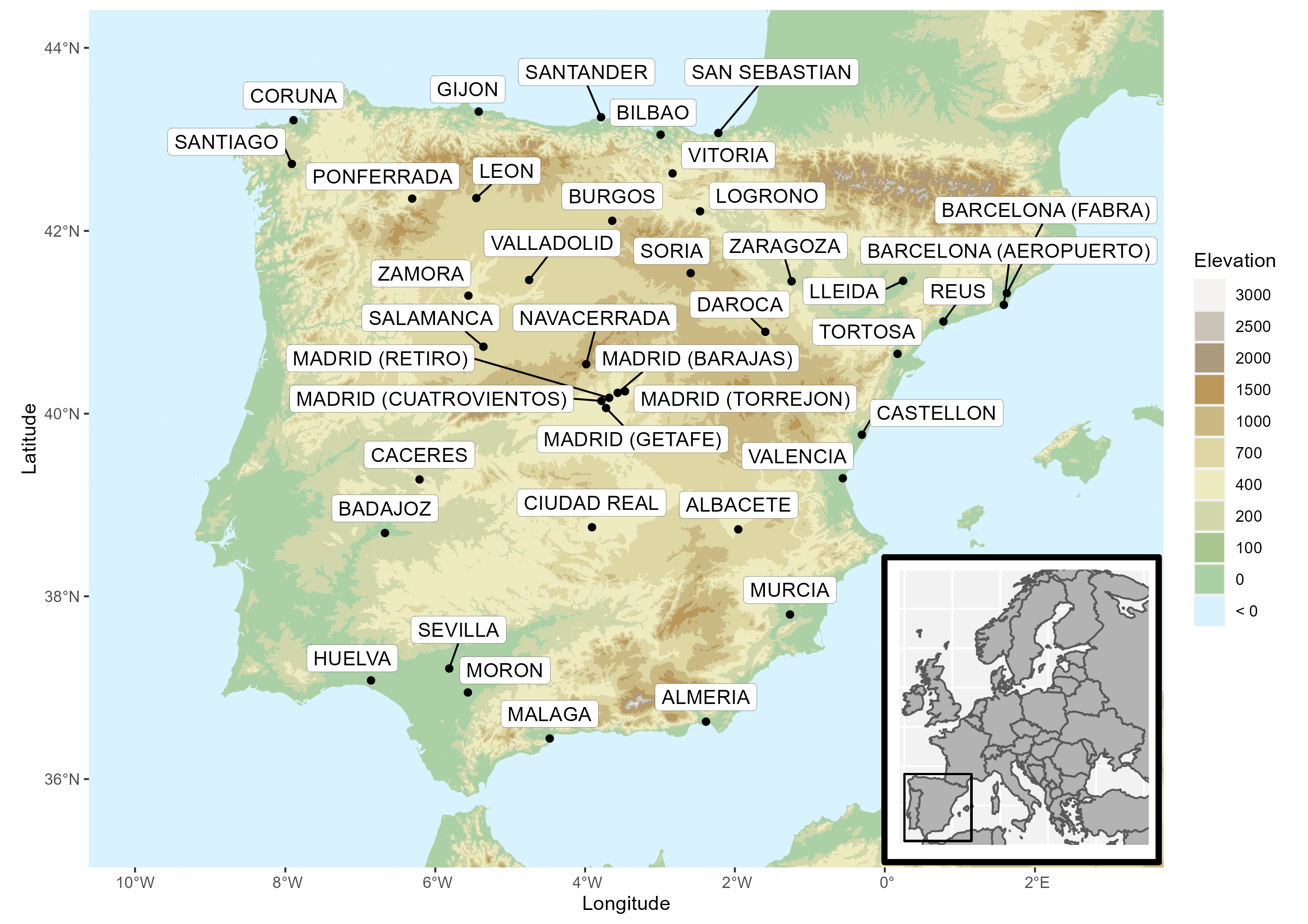
Figure 1: Map of the 40 Spanish stations in southwestern Europe.

We only included stations from the ECA&D with a minimum of $99.5\%$ reliable data over 1960–2021. There are 53 stations with this requirement over peninsular Spain, but 13 of them are removed from the dataset because they do not meet additional quality criteria as described in Section 1.1 of the Supplementary material. The retained stations have a small amount of missingness, on average, $0.07\%$ missing values. To address this, we assigned a value of $-\infty$ to missing data. Consequently, missing values are only considered records if they appear at $t=1$. A simulation study shows that the impact of this missing data on our results is negligible; see Section 1.2 of the Supplementary material.

2.2 Data precision and tied records

Spanish temperature series available in ECA&D are provided by AEMET and they are measured to the nearest $1/10$th of a ^∘C. This rounding/discretization results in some ties when records are identified. To deal with ties, an observation that is at least as large as any previous observation is called a weak record (Arnold et al., 1998, Chapter 2). Here, we define a tied record in terms equal rather than higher or equal, i.e., an $r$-tied record ($r\geq 2$) arises when an observation shares the same value with $r-1$ preceding weak records. A $3$-tied record has the same value as the two tied previous weak records. The record before this $3$-tied record was a $2$-tied record, the record before that was a record in the classical sense, and the three of them are weak records.

Among all non-trivial and weak records, the proportion of tied records across stations ranges from $4.2\%$ to $13.5\%$, with a station-wise average of $7.4\%$. The proportion of ties is almost constant across years. Out of a total of $890,600$ observations after the first trivial year, $58,981$ are classified as records, $4,352$ are $2$-tied records, $340$ are $3$-tied records, $30$ are $4$-tied records, and only $4$ are $5$-tied records.

To accommodate the tied records within the Bayesian framework, we assume that each of the true daily temperatures roundings are i.i.d., following a distribution on the interval $(\text{observed}-0.05,\text{observed}+0.05)$. Therefore, for an $r$-tied record in the rounded data series, the probability of it being a record in the true daily temperature series is $1/r$. Indicators corresponding to $r$-tied records are sampled from their $\text{Bernoulli}(1/r)$ distribution at the beginning of each iteration of the MCMC model fitting algorithm.

2.3 Exploring the occurrence of records

An exploratory analysis was conducted to evaluate departures from stationarity in the occurrence of records, identify related regressors, and enable a data-driven variable selection for the model. The covariates studied as fixed effects aim to capture spatio-temporal variability; i.e., annual trend, persistence (dependence on previous days), seasonal behavior, and geographic features. For simplicity, indicators associated with tied records are assigned a value of $0$ in this exploratory analysis. In order to avoid an over-representation of the Madrid region, where there are five stations, only the Retiro series is included in the exploratory analysis, but all of them are used for model fitting in Section 3.

Two types of exploratory tools are used in the analysis: (i) graphical tools, and (ii) exploratory global or local logit models whose response is the vector resulting from stacking the record indicator variables $I_{t\ell}(\textbf{s})$ from all or individual observed sites, respectively. Models with different regressors are compared using the AIC as a goodness of fit measure. This comparison is used to confirm or not the need for the considered temporal and spatial fixed effects; see Section 1.3.4 of the Supplementary material.

Linear predictor	AIC
$\text{offset}(-\log(t-1))-1$	343369.2
$\log(t-1)$	342238.3
$\text{poly}(\log(t-1),2)$	340112.8
$+\text{ persistence terms}$	293101.5
$+\text{ seasonal terms}$	292821.8
$+\text{ spatial terms}$	292030.7

Table 1: Nested fixed effects models and AIC; see Table 3 of the Supplementary material.

Non-stationarity.

The probability of record at time $t$ depends on $t$ (again, $p_{t}=1/t$ in the stationary case). Consequently, a model in the logit scale must at least include a trend term $\log(t-1)$, which in the stationary case would have a coefficient roughly equal to $-1$. To explore whether that term is enough to capture temporal evolution across years, the top left plot in Figure 2 shows $t\times\hat{p}_{t}$ against $t$, whose expected value under stationarity is $1$. An empirical estimate of $p_{t}$ is obtained by averaging across space and days within year, $\hat{p}_{t}=\sum_{i=1}^{36}\sum_{\ell=1}^{365}I_{t\ell}(\textbf{s}_{i})/(36\times 365)$. The plot shows a strong deviation from $1$ starting around $t=21$ (year 1980) and going up to $2$ in the final years, suggesting that probabilities of record are much higher than in a stationary climate. To allow a flexible modeling of the deviation from stationarity, the inclusion of a polynomial function of $\log(t-1)$ is considered. The first three rows in Table 1 show the AIC for three logit models including an offset $-\log(t-1)$, the covariate $\log(t-1)$, and the first and second degree orthogonal polynomials of $\log(t-1)$. According to the AIC, a third order polynomial is unnecessary and the second is preferred; see also Table 3 of the Supplementary material.

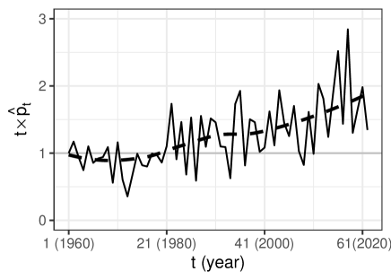
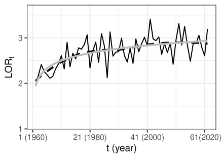
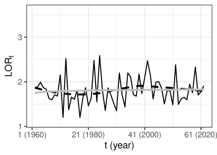
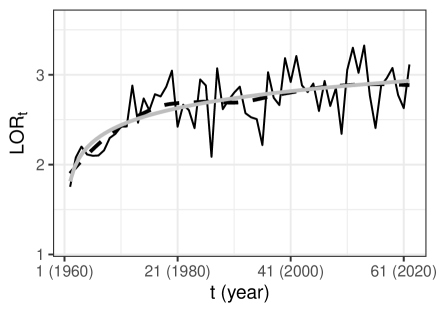
Figure 2: Top–Left: Evolution of $t\times\hat{p}_{t}$ against $t$ with reference value $1$. Top–Right: $LOR_{t}$ comparing the probability of record given a record the previous day and the probability of record without a record the previous day. Bottom–Left: $LOR_{t}$ comparing the probabilities $p_{t\mid 11}$ and $p_{t\mid 01}$. Bottom–Right: $LOR_{t}$ comparing the probabilities $p_{t\mid 10}$ and $p_{t\mid 00}$. Gray lines are linear models fitted to $\log(t-1)$ (except Top–Left) and dashed lines are LOESS curves.

In series that are not i.i.d., especially those with an underlying trend like daily temperatures under global warming, the probability of record is a function of time that can vary across series with different distributions, e.g., across series from different locations or measured on different days. The following exploratory analysis assesses which spatio-temporal factors interact with that function, in particular with $\log(t-1)$. Another important feature to study in the exploratory analysis is the existence of temperature persistence, i.e., whether the probability of a record depends on the occurrence of records on previous days.

Persistence.

To study the dependence between the occurrence of records in two consecutive days, we consider the joint distribution $[I_{t\ell}(\textbf{s}),I_{t,\ell-1}(\textbf{s})]$ expressed in terms of $2\times 2$ tables. The evolution of this dependence across years is studied with two-way tables obtained by summing across space and days within year; see Section 1.3.1 of the Supplementary material. The empirical log OR’s provide a useful tool for learning about persistence for both records and non-records,

$$LOR_{t}=\log\frac{(n_{t,11}+0.5)(n_{t,00}+0.5)}{(n_{t,01}+0.5)(n_{t,10}+0.5)},$$

where $n_{t,jk}=\sum_{i=1}^{36}\sum_{\ell=1}^{365}\textbf{1}(I_{t\ell}(\textbf{s}_{i})=j,I_{t,\ell-1}(\textbf{s}_{i})=k)$ for $j,k\in\{0,1\}$ denotes the frequencies in each cell of the table, and $0.5$ is a customary continuity correction. For notation convenience $I_{t0}(\textbf{s})\equiv I_{t-1,365}(\textbf{s})$. The $LOR_{t}$ above compares the probabilities of record given a record or a non-record the previous day. Values close to $0$ express independence while positive values capture persistence. The top right plot in Figure 2 shows the $LOR_{t}$ against $t$: the values are clearly different from $0$, moving from $2$ at the beginning to $3$ at the end, indicating a strong persistence increasing across years. The linear relationship observed between $LOR_{t}$ and $\log(t-1)$ suggests the inclusion of the autoregressive term $I_{t,\ell-1}(\textbf{s})$ and the interaction $\log(t-1)\times I_{t,\ell-1}(\textbf{s})$ in the model. The interaction allows a different coefficient of $\log(t-1)$ in the model for the probabilities of record depending on whether the previous day was a record or not.

Given the strong persistence of temperature, the introduction of second-order autoregressive terms is also considered. To that end, the joint distribution $[I_{t\ell}(\textbf{s}),I_{t,\ell-1}(\textbf{s}),I_{t,\ell-2}(\textbf{s})]$, which can be captured by a $2\times 2\times 2$ table, is used to extract the conditional distribution $[I_{t\ell}(\textbf{s})\mid I_{t,\ell-1}(\textbf{s}),I_{t,\ell-2}(\textbf{s})]$. The evolution of this second-order dependence is studied across years using the four conditional probabilities of record in a day given the occurrence or not of a record one and two days ago; i.e., $p_{t\mid 11}$, $p_{t\mid 01}$, $p_{t\mid 10}$, and $p_{t\mid 00}$. Again, the analysis is based on empirical $LOR_{t}$’s calculated by summing across days within year and sites; see Section 1.3.1 of the Supplementary material. The bottom plots in Figure 2 show the $LOR_{t}$’s that compare $p_{t\mid 11}$ and $p_{t\mid 01}$, the two conditional probabilities given that two days ago there was a record, and $p_{t\mid 10}$ and $p_{t\mid 00}$, the two conditional probabilities given that two days ago there was not a record. The evolution of the two $LOR_{t}$’s is very different. The former seems constant across years but higher than $0$, and the latter is quite similar to the $LOR_{t}$ comparing probabilities $p_{t\mid 1}$ and $p_{t\mid 0}$; this similarity is clearly due to the scarce number of records. These plots suggest that different coefficients of $\log(t-1)$ should be allowed depending on the occurrence of records or not one and two days ago; i.e., $\log(t-1)\times I_{t,\ell-2}(\textbf{s})$ and $\log(t-1)\times I_{t,\ell-1}(\textbf{s})\times I_{t,\ell-2}(\textbf{s})$, and $I_{t,\ell-2}(\textbf{s})$ and $I_{t,\ell-1}(\textbf{s})\times I_{t,\ell-2}(\textbf{s})$ should be included in the model. The similarity between the LOESS curve and the fitted values of the linear model including $\log(t-1)$ suggests that interactions with higher order trend polynomials are not necessary. The AIC values in Table 1 confirm the need for the persistence terms.

Seasonality.

Many studies have found that global warming and, in particular, the increase in incidence of extreme temperatures is not homogeneous within the year. In Spain, Castillo-Mateo, Cebrián & Asín (2023b) found that the increase in the probabilities of record is significant in summer but not in autumn and relevant differences are also found between months. To allow different annual evolution for days within year, a harmonic given by the terms $\sin(2\pi\ell/365)$ and $\cos(2\pi\ell/365)$, and its interactions with the first and second degree orthogonal polynomials of $\log(t-1)$, are included in the model. The need for these terms is confirmed by the exploratory logit models in Table 1, and supported by the different patterns in $t\times\hat{p}_{t}$ lines by season in Figure 1 of the Supplementary material.

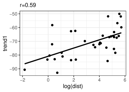
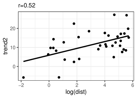
Figure 3: Estimated coefficients of the first (left) and second (right) degree orthogonal polynomials of $\log(t-1)$ in local logit models for each observed site against $\log(\operatorname{dist}(\textbf{s}))$.

Spatial variability.

The effect of global warming on the occurrence of records is not spatially homogeneous. Previous work (Coumou et al., 2013) and the characteristics of the study area suggest the need for including spatial covariates. Latitude, longitude, and elevation were explored but excluded as described in Section 1.3.3 of the Supplementary material. McBride et al. (2022) and Castillo-Mateo, Cebrián & Asín (2023b) found that the increase in the number of records was different between coastal and inland stations both in South Africa and Spain, respectively. The minimum distance to the coast was incorporated into the model as an interaction between the trend terms and a functional form of distance to the coast in km, $\operatorname{dist}(\textbf{s})$. A suitable expression was identified by fitting, for each observed site, local logit models with the covariates above (trend, persistence, and seasonality). The relationship between the estimated coefficients of the trend terms for each site and different functions of $\operatorname{dist}(\textbf{s})$ were explored. Figure 3 shows a linear relationship between those coefficients and $\log(\operatorname{dist}(\textbf{s}))$. Analogous results were obtained for the interaction between the persistence terms and $\log(\operatorname{dist}(\textbf{s}))$; see Section 1.3.3 of the Supplementary material. The AIC for the logit model with spatial terms in Table 1 confirms the need for these terms.

In summary, this exploratory analysis argues, in detail, for the specification of the fixed effects in the full logit model that includes 20 covariates. The resulting fixed effect terms are written precisely in the next section.

3 Model specifics

This section proposes a rich spatial logistic regression model across days, for annual temperature records, motivated by the exploratory analysis in Section 2.3. It provides details for model fitting and also spatial interpolation at unobserved locations, in a Bayesian framework, to extract desired posterior inference for any spatio-temporal feature of the occurrence of records. The section concludes with proposed metrics for model comparison.

3.1 Spatial modeling for record breaking

Let $I_{t\ell}(\textbf{s})$ denote the record indicator of the daily maximum temperature for day $\ell$, $\ell=1,\ldots,365$, within year $t$, $t=1,\ldots,T$, at location s, $\textbf{s}\in D$ with $D$ being peninsular Spain, for the series starting on January 1, 1960; so, $t=1$ corresponds to 1960 and $T=62$ corresponds to 2021. We model record indicators beginning with day $\ell=3,\ldots,365$, year $t=2,\ldots,T$, and location s according to

$$I_{t\ell}(\textbf{s})\mid I_{t,\ell-1}(\textbf{s}),I_{t,\ell-2}(\textbf{s})\sim\text{Bernoulli}(g^{-1}(\eta_{t\ell}(\textbf{s})))\quad\text{with}\quad\eta_{t\ell}(\textbf{s})=\textbf{x}_{t\ell}(\textbf{s})\mbox{\boldmath$\beta$}+w_{t\ell}(\textbf{s}),$$ (1)

where $g(p)=\log\{p/(1-p)\}$ is the logit link function. Here, $p_{t\ell}(\textbf{s})=g^{-1}(\eta_{t\ell}(\textbf{s}))$ is the probability of a record for day $\ell$, year $t$, and location s, with fixed effects $\textbf{x}_{t\ell}(\textbf{s})\mbox{\boldmath$\beta$}$ and random effects $w_{t\ell}(\textbf{s})$. The $\textbf{x}_{t\ell}(\textbf{s})=(1,x_{t\ell 1}(\textbf{s}),\ldots,x_{t\ell k}(\textbf{s}))$ are $k+1$ covariates measured on day $\ell$, year $t$, and location s with $\beta$ a column vector of length $k+1$ of regression coefficients. The $w_{t\ell}(\textbf{s})$ are space-time correlated errors.

We first supply the fixed effects component. Apart from the intercept, the entries are:

• $\operatorname{trend1}_{t}$ and $\operatorname{trend2}_{t}$, denoting the first and second degree orthogonal polynomials of $\log(t-1)$; they enrich the trend in the probabilities of record across $t$ beyond the trend under a stationary climate.

• persistence terms to capture first and second order autoregressive dependence, $I_{t,\ell-1}(\textbf{s})$, $I_{t,\ell-2}(\textbf{s})$, and $I_{t,\ell-1}(\textbf{s})\times I_{t,\ell-2}(\textbf{s})$, and their interactions with $\log(t-1)$; this means that different intercepts and first-order time trends are allowed for each of the four possible persistence situations defined by the occurrence or not of records in each of the two previous days.

• seasonal terms including one harmonic, $\sin_{\ell}=\sin(2\pi\ell/365)$ and $\cos_{\ell}=\cos(2\pi\ell/365)$, and their interactions with the trend across years; these terms allow for seasonality in the probability of records within the year and enable it to vary across years.

• spatial terms to enrich the effect of $\log(\operatorname{dist}(\textbf{s}))$ including interaction with trend across years and with persistence; the effect of distance from the coast varies with yearly trend and also according to persistence in the previous two days.

In summary, we have the intercept and the following 20 predictors:

$$\textbf{x}_{t\ell}(\textbf{s})=( 1,\operatorname{trend1}_{t},\operatorname{trend2}_{t},I_{t,\ell-1}(\textbf{s}),I_{t,\ell-2}(\textbf{s}),I_{t,\ell-1}(\textbf{s})\times I_{t,\ell-2}(\textbf{s}),$$

$$\log(t-1)\times I_{t,\ell-1}(\textbf{s}),\log(t-1)\times I_{t,\ell-2}(\textbf{s}),\log(t-1)\times I_{t,\ell-1}(\textbf{s})\times I_{t,\ell-2}(\textbf{s}),$$

$$\sin_{\ell},\cos_{\ell},\sin_{\ell}\times\operatorname{trend1}_{t},\cos_{\ell}\times\operatorname{trend1}_{t},\sin_{\ell}\times\operatorname{trend2}_{t},\cos_{\ell}\times\operatorname{trend2}_{t}$$

$$\log(\operatorname{dist}(\textbf{s})),\log(\operatorname{dist}(\textbf{s}))\times\operatorname{trend1}_{t},\log(\operatorname{dist}(\textbf{s}))\times\operatorname{trend2}_{t},$$

$$\log(\operatorname{dist}(\textbf{s}))\times I_{t,\ell-1}(\textbf{s}),\log(\operatorname{dist}(\textbf{s}))\times I_{t,\ell-2}(\textbf{s}),\log(\operatorname{dist}(\textbf{s}))\times I_{t,\ell-1}(\textbf{s})\times I_{t,\ell-2}(\textbf{s})).$$

While 20 fixed effects terms may seem excessive, in explaining the roughly $900,000$ observations we do find all of them significant using the foregoing fixed effects logistic regression variable selection, with further support from the results in Section 4.2.

We introduce explicit spatial and temporal dependence through random effects. Possibilities for modeling $w_{t\ell}(\textbf{s})$ include: (i) a spatially-varying intercept, $w_{t\ell}(\textbf{s})=w(\textbf{s})$; (ii) an additive form with annual intercepts, $w_{t\ell}(\textbf{s})=w(\textbf{s})+w_{t}$; (iii) daily intercepts, $w_{t\ell}(\textbf{s})=w(\textbf{s})+w_{t\ell}$; and (iv) daily-spatially-varying intercepts, $w_{t\ell}(\textbf{s})$. From (i) to (iii), spatial dependence is captured by $w(\textbf{s})$ to provide local adjustments to the global intercept. It is supplied as a mean-zero Gaussian process with an exponential covariance function such that $\operatorname*{cov}(w(\textbf{s}),w(\textbf{s}^{\prime}))=\sigma_{0}^{2}\exp\{-\phi_{0}\lvert\lvert\textbf{s}-\textbf{s}^{\prime}\rvert\rvert\}$, where $\sigma_{0}^{2}$ and $\phi_{0}$ are, respectively, the variance and decay parameters of the Gaussian process, and $\lvert\lvert\textbf{s}-\textbf{s}^{\prime}\rvert\rvert$ is the distance between s and $\textbf{s}^{\prime}$. Temporal dependence is captured by $w_{t}$ or $w_{t\ell}$. These processes are modeled as $w_{t}\sim N(0,\sigma_{1}^{2})$ or $w_{t\ell}\sim N(0,\sigma_{1}^{2})$, respectively. An autoregressive specification is unnecessary for these $w$’s. That is, we implemented autoregression across years and found no significance while daily autoregression is already accounted for in the covariates. The full model (iv) imposes the most demanding implementation, modeling $w_{t\ell}(\textbf{s})$ as Gaussian processes with mean $w_{t\ell}$ and a common exponential covariance function having variance and decay parameters $\sigma_{0}^{2}$ and $\phi_{0}$, as above.

For prediction, the autoregressive model requires an initial condition for $I_{t1}(\textbf{s})$ and $I_{t2}(\textbf{s})$, the first and second values in year $t$. Given the inherent break for each year $t$, we employ a distinct linear specification for modeling these indicators compared to (1). We model them as $\eta_{t1}(\textbf{s})=\textbf{x}_{t1}(\textbf{s})\mbox{\boldmath$\beta$}_{1}+w_{t1}(\textbf{s})$ and $\eta_{t2}(\textbf{s})=\textbf{x}_{t2}(\textbf{s})\mbox{\boldmath$\beta$}_{2}+w_{t2}(\textbf{s})$. The covariate vectors are reduced to $\textbf{x}_{t1}(\textbf{s})=(1,\operatorname{trend1}_{t},I_{t-1,365}(\textbf{s}))$ and $\textbf{x}_{t2}(\textbf{s})=(1,\operatorname{trend1}_{t},I_{t1}(\textbf{s}))$. The $w_{t\ell}(\textbf{s})$ are modeled as above, each a Gaussian process with mean $w_{t\ell}\sim N(0,\sigma_{1,\ell}^{2})$ and exponential covariance function having variance $\sigma_{0,\ell}^{2}$ and the same decay parameter $\phi_{0}$.

3.2 Prior specification and model fitting

Prior distributions.

Model inference is implemented in a Bayesian framework. Adopting the data augmentation approach described below, we can use the same conjugate priors as in a standard geostatistical linear model with normal errors. We assign proper but weakly informative priors as follows. Let $\textbf{v}\sim N_{n}(\mbox{\boldmath$\mu$},\mbox{\boldmath$\Sigma$})$ be an $n$-dimensional random vector that follows a multivariate normal distribution with mean vector $\mu$ and positive-definite covariance matrix $\Sigma$. Let $\textbf{1}_{n}$ ($\textbf{0}_{n}$) be the $n$-dimensional vector of ones (zeros) and $\textbf{I}_{n}$ the $n\times n$-dimensional identity matrix. The regression coefficients are assigned $\mbox{\boldmath$\beta$}\sim N_{k+1}(\mbox{\boldmath$\mu$}_{\bm{\beta}},\mbox{\boldmath$\Sigma$}_{\bm{\beta}})$ with mean $\mbox{\boldmath$\mu$}_{\bm{\beta}}=\textbf{0}_{k+1}$ and covariance $\mbox{\boldmath$\Sigma$}_{\bm{\beta}}=100^{2}\textbf{I}_{k+1}$. Equivalently, $\mbox{\boldmath$\beta$}_{\ell}\sim N_{3}(\mbox{\boldmath$\mu$}_{\bm{\beta}_{\ell}},\mbox{\boldmath$\Sigma$}_{\bm{\beta}_{\ell}})$ with mean $\mbox{\boldmath$\mu$}_{\bm{\beta}_{\ell}}=\textbf{0}_{3}$ and covariance $\mbox{\boldmath$\Sigma$}_{\bm{\beta}_{\ell}}=100^{2}\textbf{I}_{3}$ for days $\ell=1,2$. The coefficient associated with $\log(t-1)$ could have a prior mean of $-1$ corresponding to a stationary climate but with the large prior variance there would be no practical difference in posterior inference. The variance parameters are each assigned an inverse gamma distribution, i.e., $\sigma_{0}^{2},\sigma_{0,\ell}^{2},\sigma_{1}^{2},\sigma_{1,\ell}^{2}\sim IG(a_{\sigma},b_{\sigma})$ with shape parameter $a_{\sigma}=2$ and scale parameter $b_{\sigma}=1$.

Finally, we assign a gamma prior to the decay parameter $\phi_{0}\sim G(a_{\phi},b_{\phi})$ where $a_{\phi}=2$ and $b_{\phi}=1$ as above. A prior considering the effective range, $3/\phi_{0}\sim IG(a_{\phi},3b_{\phi})$, the distance beyond which spatial association becomes negligible, could set $a_{\phi}=2$ and $b_{\phi}=100$. This prior has a mean of $300$ km, roughly one-third of the maximum pairwise site distances, with infinite variance, and puts $90\%$ of the mass in $(63.2,844.2)$ km. With this last prior, the posterior distribution placed the majority of its mass on relatively large values for the effective range, so we ultimately opted for the prior with the “constraint” $3$ km mean and infinite variance. With the large amount of data, we did not find any inference sensitivity to the mean of this prior, or to the hyperparameters of the prior distribution for the regression or variance parameters.

Data augmentation approach.

Specification of the logit model in (1), following Held & Holmes (2006) using latent standard logistic variables, leads to the augmented model $I_{t\ell}(\textbf{s})=1$ if $Y_{t\ell}(\textbf{s})>0$ and $0$ otherwise. Here, $Y_{t\ell}(\textbf{s})=\textbf{x}_{t\ell}(\textbf{s})\mbox{\boldmath$\beta$}+w_{t\ell}(\textbf{s})+\epsilon_{t\ell}(\textbf{s})$ where we have i.i.d. $\epsilon_{t\ell}(\textbf{s})\sim N(0,\lambda_{t\ell}(\textbf{s}))$, $\lambda_{t\ell}(\textbf{s})=(2K_{t\ell}(\textbf{s}))^{2}$, and $K_{t\ell}(\textbf{s})\sim KS$ follows the asymptotic distribution of the Kolmogorov-Smirnov statistic. In this case, $\epsilon_{t\ell}(\textbf{s})$ follows a scale mixture of normal form with a marginal logistic distribution, so that the posterior distribution of the model parameters for the augmented model and for model (1) are equivalent. The advantage of working with this representation is that we have the usual conjugacy for the model parameters given the latent $Y_{t\ell}(\textbf{s})$’s. Computational details of the MCMC algorithm used to fit the full model are given in Section 2 of the Supplementary material. An alternative data augmentation approach for fitting Bayesian logistic regression models uses Pólya-gamma latent variables (Polson et al., 2013).

It is worth noting that the specification above implies spatial dependence at the second modeling stage. That is, the $I_{t\ell}(\textbf{s})$’s are conditionally independent with $P(I_{t\ell}(\textbf{s})=1\mid\lambda_{t\ell}(\textbf{s}))=\Phi((\textbf{x}_{t\ell}(\textbf{s})\mbox{\boldmath$\beta$}+w_{t\ell}(\textbf{s}))/\lambda_{t\ell}^{1/2}(\textbf{s}))$ where $\Phi$ is the cdf of the standard normal distribution, but marginally, they are dependent with direct calculation of the dependence structure available. We are adopting the customary way of introducing spatial dependence in the geostatistical generalized linear model which introduces two sources of error (Diggle et al., 1998). As far as the realized surfaces are concerned, $Y_{t\ell}(\textbf{s})$ and $I_{t\ell}(\textbf{s})$ are everywhere discontinuous.

We could make the $Y_{t\ell}(\textbf{s})$ surface continuous by removing the $\epsilon_{t\ell}(\textbf{s})$. Then, marginalizing over $w_{t\ell}(\textbf{s})$ after carefully modifying its covariance function to ensure it follows a marginal standard logistic distribution, the indicator surface would be smooth with countable discontinuities. However, in practice, it is not sensible to argue that the model with only spatial residuals explains the responses perfectly; we almost always envision some pure error which we pass on to the indicator process. In different words, the conditional independence concern is related to what is typically referred to as “micro-scale” dependence (see, e.g., Banerjee et al., 2014, Chapter 6). After we condition on the spatial random effects, we may still retain some fine-scale spatial dependence which we are modeling as noise. Such dependence is known to be difficult to extract and, in the context of our very rich modeling for the indicator functions, will not affect inference.

3.3 Spatial interpolation and inference

Spatial interpolation.

Our inference objective is the posterior predictive distribution for the record indicators (or their probabilities) for any location in the study region within the observed time period, i.e., for $I_{t\ell}(\textbf{s}_{0})$ (or $p_{t\ell}(\textbf{s}_{0})$) for any $\textbf{s}_{0}\in D$. From (1), a posterior sample from $I_{t\ell}(\textbf{s}_{0})$ can be obtained by sampling from a Bernoulli distribution with probability $p_{t\ell}(\textbf{s}_{0})$. A sample of $p_{t\ell}(\textbf{s}_{0})$ is obtained through the inverse link function taking a sample of the linear predictor $\eta_{t\ell}(\textbf{s}_{0})$, which is a function of the model parameters and process realizations. Posterior samples for the parameters are available from each iteration of the MCMC algorithm, and posterior samples for the spatial processes are available using posterior samples of the parameters through usual Bayesian kriging (Banerjee et al., 2014, Chapter 6). Sampling must be done dynamically in $t$ and $\ell$ because the response variable depends on its own previous values.

Model-based tools.

Employing $G_{D}$, a fine spatial grid for $D$, posterior samples from $I_{t\ell}(\textbf{s})$ can be realized at each location in $G_{D}$ for every day $\ell$, $\ell=1,\ldots,365$, within year $t$, $t=2,\ldots,T$. So, we can make inference about any feature of interest related to the occurrence of records. Let $1\leq\ell_{1}\leq\ell_{2}\leq 365$ and $1\leq t_{1}\leq t_{2}\leq T$. Then, a general feature of primary interest is the average cumulative number of records across days from $\ell_{1}$ to $\ell_{2}$ and across years from $t_{1}$ to $t_{2}$. It is defined as

$$\bar{N}_{t_{1}:t_{2},\ell_{1}:\ell_{2}}(\textbf{s})=\frac{1}{\ell_{2}-\ell_{1}+1}\sum_{t=t_{1}}^{t_{2}}\sum_{\ell=\ell_{1}}^{\ell_{2}}I_{t\ell}(\textbf{s}).$$ (2)

The average total number of records $\bar{N}_{T}(\textbf{s})$ arises with $\ell_{1}=1$, $\ell_{2}=365$, $t_{1}=1$ and $t_{2}=T$. Also of interest is the number of records in the observed period of the 21st century and its comparison across seasons, leading to the statistics $\bar{N}_{(T-21):T,\text{DJF}}(\textbf{s})$, $\bar{N}_{(T-21):T,\text{MAM}}(\textbf{s})$, $\bar{N}_{(T-21):T,\text{JJA}}(\textbf{s})$, and $\bar{N}_{(T-21):T,\text{SON}}(\textbf{s})$, where DJF is winter (December, January, and February), MAM is spring, JJA is summer, and SON is autumn, with obvious notation. Other periods of interest could be the months of the past decade.

Comparison between the average number of records predicted by the model and the expected number of records under the stationary case, $E_{0}[\bar{N}_{t_{1}:t_{2},\ell_{1}:\ell_{2}}(\textbf{s})]=\sum_{t=t_{1}}^{t_{2}}1/t$ may be of interest. The ratio expression

$$R_{t_{1}:t_{2},\ell_{1}:\ell_{2}}(\textbf{s})=\frac{\bar{N}_{t_{1}:t_{2},\ell_{1}:\ell_{2}}(\textbf{s})}{E_{0}[\bar{N}_{t_{1}:t_{2},\ell_{1}:\ell_{2}}(\textbf{s})]},$$ (3)

captures records expected by the model compared to a scenario without climate change.

Computing the above quantities for all $\textbf{s}\in G_{D}$ we can draw maps of the posterior mean or borders of the $90\%$ credible intervals (CI’s) of the quantities of interest. This enables a useful picture of the spatio-temporal characteristics of the occurrence of records and assessment of regions and time periods with higher risk of exceeding temperatures above all of the previous measurements.

In a different direction, consider the extent of record surface (ERS) over a block $B\subseteq D$ of peninsular Spain for a given day $\ell$ within a given year $t$ (see Cebrián, Asín, Gelfand, Schliep, Castillo-Mateo, Beamonte & Abaurrea, 2022, for more details of the concept of extent). Suppose we compute

$$\widehat{\text{ERS}}_{t\ell}(B)=\frac{1}{\lvert G_{B}\rvert}\sum_{\textbf{s}_{j}\in G_{B}}I_{t\ell}(\textbf{s}_{j}),$$ (4)

where $G_{B}$ is a fine spatial grid of $B$ and $\lvert G_{B}\rvert$ is the number of grid cells in $G_{B}$. We define $ERS_{t\ell}(B)$ as the limit of this expression as the size of the grid cells go to $0$. We interpret the limit as the proportion of $B$ which produced a record on day $\ell$ in year $t$.

We could compute $\widehat{\text{ERS}}_{t\ell}(B)$ for different blocks $B_{1},B_{2}\subseteq D$ to compare trends in different subregions. Also, we can compute it for all of peninsular Spain, $D$, that would be the proportion of the country which is suffering a record-breaking temperature event on day $\ell$ within year $t$. Following the above notation, we can go further and average these amounts for all or some $\ell$’s giving rise to a yearly evolution of the average number of records all over $B$, say $\widehat{\overline{\text{ERS}}}_{t}(B)$. Again, we can plot the posterior mean and $90\%$ CI of $t\times\widehat{\overline{\text{ERS}}}_{t}(B)$ against $t=1,\ldots,T$ to assess the nature of deviations from $1$. Alternatively, the cumulative sum of $\widehat{\overline{\text{ERS}}}_{t}(B)$ in $t=1,\ldots,T$ could be drawn as the proportion of the total number of records across the entire region.

3.4 Model comparison and checking

The performance of the models for record-breaking is compared using metrics for cross-validation and for the deviance. Both approaches globally evaluate the goodness of fit of the models. The adequacy of the selected model is criticized using posterior predictive checks for features of interest.

Cross-validation.

Model comparison is considered in the context of performance of the interpolation across the 40 locations. In particular, the models are compared using 10-fold cross-validation. This means that the dataset is split at random into 10 groups with data from four different sites for each group; see Section 3.1 of the Supplementary material. Then, each group of four sites is taken as hold-out and the model is fitted with the remaining 36 sites. Finally, posterior samples from the conditional probabilities of record for the hold-out sites are obtained using one-step ahead prediction. This is doable since the $I_{t,\ell-1}(\textbf{s})$ and $I_{t,\ell-2}(\textbf{s})$ to condition on are known (or we use the data rounding strategy for indicators associated to tied records). Indicators associated with tied records are not included in the metrics because we do not know their true value.

Here, we consider two metrics for comparing model performance and a third metric is given in Section 3.1 of the Supplementary material. The first of these is based on the Brier score (BS; Brier, 1950) which, for binary events, is a strictly proper scoring rule (Czado et al., 2009) given by the squared difference $[I_{t\ell}(\textbf{s})-\hat{p}_{t\ell}(\textbf{s})]^{2}$, where $\hat{p}_{t\ell}(\textbf{s})$ is the posterior mean of the probability of record on day $\ell$ within year $t$ at a location s in a group given data in the remaining nine groups of locations. We average the BS’s over all observations, and a lower score indicates better performance. Since the BS penalizes false negatives and false positives equally, it may not be the most suitable metric for record-breaking events because of the unbalanced nature of the data. As a consequence, we also consider the area under the receiver operating characteristic curve (AUC) obtained via the R package pROC (Robin et al., 2011) for each held-out group one by one. We average the AUC’s across all groups; its value ranges from $0$ to $1$ and a higher value indicates better performance.

Deviance.

Model comparison is also considered in terms of deviance. A commonly used measure in this regard for Bayesian models is the deviance information criterion (DIC; Spiegelhalter et al., 2002) which is the sum of two components, one for quantifying the model fit and the other for penalizing its complexity; see Section 3.2 of the Supplementary material. Models with smaller DIC are better supported by the data.

Posterior predictive checks.

Model adequacy is criticized in terms of calibration and sharpness of the probabilistic forecasts or predictions. Scatter plots that display the actual observations for particular features versus a summary of their corresponding predictive distributions based on the posterior mean and $90\%$ CI are useful to observe the consistency between the predictions and the observations together with the concentration of the predictive distributions.

Another diagnostic tool to identify model deficiencies is the probability integral transform (PIT). This is the value that the posterior cdf attains at an observation. If the observation is drawn from the predictive distribution and the distribution is continuous, the PIT has a standard uniform distribution. Here, we adapt the PIT histogram for discrete data proposed by Czado et al. (2009); see Section 3.3 of the Supplementary material.

4 Results

We first present model comparison with differing inclusion of the foregoing spatial and temporal dependence introduced in Section 3.1 and model checking for the selected model. Then, we present the results for the full model over peninsular Spain.

The models were fitted by scaling the covariates to have zero mean and unit variance to improve the mixing of the MCMC. For each model we ran two chains of the MCMC algorithm, each chain with different initial values, each to $200,000$ iterations for the full model (smaller models require fewer iterations), to obtain samples from the joint posterior distribution. The first half of the samples were discarded as burn-in and the remaining samples were thinned to $500$ samples from each chain. Section 4 of the Supplementary material contains usual convergence diagnostics for the MCMC samples.

4.1 Model comparison and checking

Model comparison.

The metrics in Section 3.4 are used to compare the models in Table 2 (BS, AUC, and DIC) using 10-fold cross-validation and the deviance. The models include the fixed effects already discussed; they differ from each other in the spatial and temporal random effects described in Section 3.1, with the full model $M_{5}$ being the richest specification. Comparison with the stationary model $M_{0}$ is solely for illustration. With regard to the cross-validation model performance metrics, two periods for record breaking are considered. The first employs the first 30 years of the series when records are more frequent; the second employs the last 31 years of the series when records are more rare.

Model	Linear predictor	BS 1	BS 2	AUC 1	AUC 2	DIC
$M_{0}$	$\eta_{t\ell}(\textbf{s})=-\log(t-1)$	$7.88$	$3.23$	$0.733$	$0.514$	$393805.4$
$M_{1}$	$\eta_{t\ell}(\textbf{s})=\textbf{x}_{t\ell}(\textbf{s})\mbox{\boldmath$\beta$}$	$6.49$	$2.91$	$0.831$	$0.686$	$333193.6$
$M_{2}$	$\eta_{t\ell}(\textbf{s})=\textbf{x}_{t\ell}(\textbf{s})\mbox{\boldmath$\beta$}+w(\textbf{s})$	$6.49$	$2.91$	$0.831$	$0.687$	$333130.3$
$M_{3}$	$\eta_{t\ell}(\textbf{s})=\textbf{x}_{t\ell}(\textbf{s})\mbox{\boldmath$\beta$}+w(\textbf{s})+w_{t}$	$6.46$	$2.90$	$0.837$	$0.716$	$331142.9$
$M_{4}$	$\eta_{t\ell}(\textbf{s})=\textbf{x}_{t\ell}(\textbf{s})\mbox{\boldmath$\beta$}+w(\textbf{s})+w_{t\ell}$	$5.20$	$2.48$	$0.924$	$0.904$	$251653.5$
$M_{5}$	$\eta_{t\ell}(\textbf{s})=\textbf{x}_{t\ell}(\textbf{s})\mbox{\boldmath$\beta$}+w_{t\ell}(\textbf{s})$	$4.32$	$2.13$	$0.944$	$0.924$	$182680.2$

Table 2: The different nested models compared and their corresponding metrics. Metrics: $100\times\text{BS}$ and AUC 1 in 1961–1990 and 2 in 1991–2021, and DIC.

Each dependence component included improves the performance of the model, with the full model being the best in all metrics. The most significant improvements are produced by the inclusion of covariates and the inclusion of daily-varying intercepts. However, the daily spatial effects also lead to a substantial gain. The cross-validation AUC values higher than $0.9$ for the full model, even for the period 1991–2021, indicate that the model has excellent ability to explain incidence of record and non-record events. The two parts of the DIC to account for model fit and complexity are shown in Table 4 of the Supplementary material. Additional disaggregated AUC’s for the full model by decade, season and location are shown in Figure 8 of the Supplementary material; which is useful to know periods of time or spatial regions that the model reproduces better or worse. In general, performance is homogeneous between decades and seasons, while there is some differences between locations. Most AUC’s are greater than $0.9$, except for Málaga and Almería, the two southernmost weather stations, which present some difficulties probably due to their orography.

Model checking.

The posterior predictive checks assess the adequacy of the full model for explaining record-breaking occurrences. Figure 9 of the Supplementary material shows the scatter plot and associated PIT histogram of $R_{53:62,month}(\textbf{s})$ in (3) for each observed location and $month$ going through the $12$ months. The same is shown for $t\times\widehat{\overline{\text{ERS}}}_{t,season}(D)$ averaging in (4) (defined over the grid of $40$ observed locations) for $t=2,\ldots,T$ going through the $4$ seasons. The discussion and figure in the Supplementary material effectively demonstrate very good model adequacy.

4.2 Inference

Here, we show results for the full model. First, a summary of the posterior distribution of the regression coefficients and other hyperparameters. Then, the model-based tools from Section 3.3 are used to make inference on the record-breaking events over peninsular Spain.

Posterior distribution of the model parameters.

The posterior mean and $90\%$ CI of the regression coefficients from the full model, with scaled covariates, are shown in Figure 4. No CI includes zero except for the interaction between $\cos_{\ell}$ and $\operatorname{trend2}_{t}$. For ease of interpretation, Table 5 of the Supplementary material includes the posterior mean and $90\%$ CI for all model parameters, but expressed in terms of non-scaled covariates. Here, we analyze the OR’s associated with persistence terms, and the hyperparameters. The trend is further studied below using model-based tools.

The posterior distribution of parameters associated with $I_{t,\ell-1}(\textbf{s})$, $I_{t,\ell-2}(\textbf{s})$, and their interactions reveals a big increase in the probabilities of record due to short-term dependence. This increase is higher close to the coast or in later years. For example, the occurrence of records gives an OR up to $20$ when the two previous days were records, $12$ when there was a record only on the previous day, and slightly lower than $3$ when there was a record two days ago but not the previous day; see Section 5.2 of the Supplementary material.

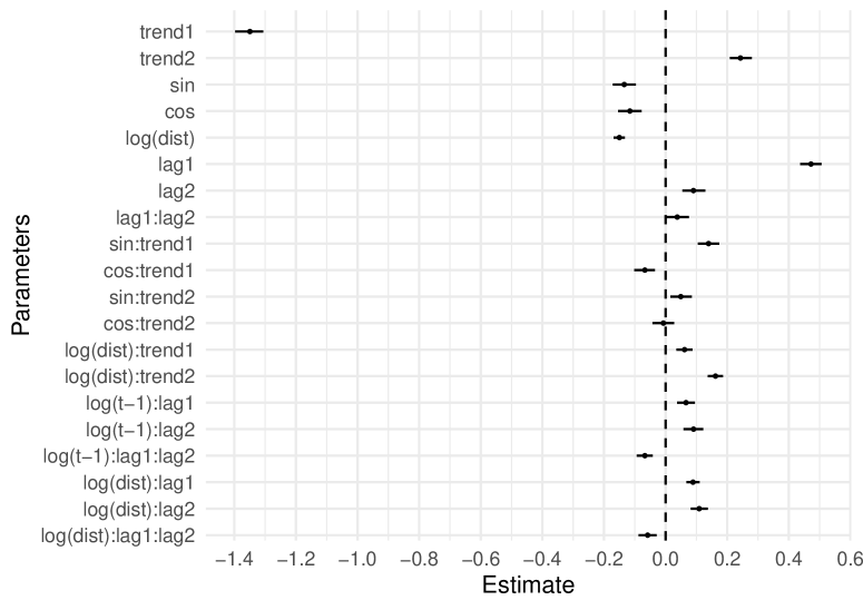
Figure 4: Posterior mean and $90\%$ CI of the $\bm{\beta}$ coefficients from the full model with scaled covariates. lag1 and lag2 denote the covariates $I_{t,\ell-1}(\textbf{s})$ and $I_{t,\ell-2}(\textbf{s})$, respectively.

The posterior mean and $90\%$ CI for the intercept $\beta_{0}$ are $-6.90$ $(-6.98,-6.80)$. For the variances of the random effects we have $11.19$ $(10.74,11.70)$ for $\sigma_{0}^{2}$, and $2.01$ $(1.57,2.43)$ for $\sigma_{1}^{2}$. These variances give evidence of the strong daily and spatial variability in the occurrence of records. Finally, the decay parameter $\phi_{0}$ is $0.0021$ $(0.0019,0.0022)$, which gives an effective range between $1390.6$ and $1550.2$ km, yielding smooth surfaces indicating that record occurrence in even the two most distant observed sites within peninsular Spain have a correlation of $0.16$ $(0.14,0.17)$. This is in agreement with the co-occurrence of records in the region. Table 8 of the Supplementary material summarizes the posterior distribution of all the hyperparameters in the model.

Model-based analysis over peninsular Spain.

This section reports results for three of the large number of model-based tools that can be utilized to draw inferences from the model. Results from additional tools are shown in Section 5.3 of the Supplementary material. First, we need a fine grid $G_{D}$ of points within peninsular Spain, we choose $G_{D}$ with resolution of $10\text{ km}\times 10\text{ km}$ yielding $\lvert G_{D}\rvert=4,937$ grid cells. Altogether, the entire posterior predictive time series results in a very large dataset from which maps and time series are computed. For instance, we have $61$ years by $365$ days by $4,937$ grid centroids by $1,000$ replicates yielding approximately 110 billion points.

First, the total number of records $\bar{N}_{62}(\textbf{s})$ in (2) is analyzed in Figure 11 of the Supplementary material. In this regard, $90.0\%$ of the region shows a significantly higher number of records compared to the stationary case, while no points exhibit a significantly lower number of records. The Atlantic and southern Mediterranean coasts seem to have a number of records compatible with stationarity. However, we are interested in studying the number of records during the last years of the studied period, as they provide a more current picture of the climate and are not influenced by the high probability of occurrence in the early stages. Analyzing records by season is also crucial because each season has distinct spatial and temporal patterns. To quantify the occurrence of records in the past decade, Figure 5 shows the posterior mean of the ratio $R_{53:62,season}(\textbf{s})$ in (3) for years from 2012–2021 by $season$ going through the four seasons. This ratio compares the average number of records predicted by the model and the expected average number under stationarity for the desired period. The corresponding maps of the $0.05$ and $0.95$ quantiles are shown in Figure 12 of the Supplementary material. The model estimates that the global warming trends have increased the number of records expected in the past decade almost two-fold, $1.93$ $(1.89,1.98)$, which suggests that only about half as many records would have been observed in those years over peninsular Spain if the process were stationary. By season the values are $1.88$ $(1.80,1.97)$ in winter, $1.81$ $(1.72,1.89)$ in spring, $2.13$ $(2.04,2.22)$ in summer, and $1.92$ $(1.83,2.01)$ in autumn. The number of records in the past decade is higher than in the stationary case everywhere, and this difference is significant for any point in the region. The percentage of area that has a significantly higher number of records is $100\%$ for winter, $90.1\%$ for spring, $98.4\%$ for summer, and $99.9\%$ for autumn. During this period, summer presents greater warming on average but also greater spatial variability compared to, e.g., winter. Analogous are the results for the number of records in the 21st century (2000–2021) in Figure 13 of the Supplementary material.

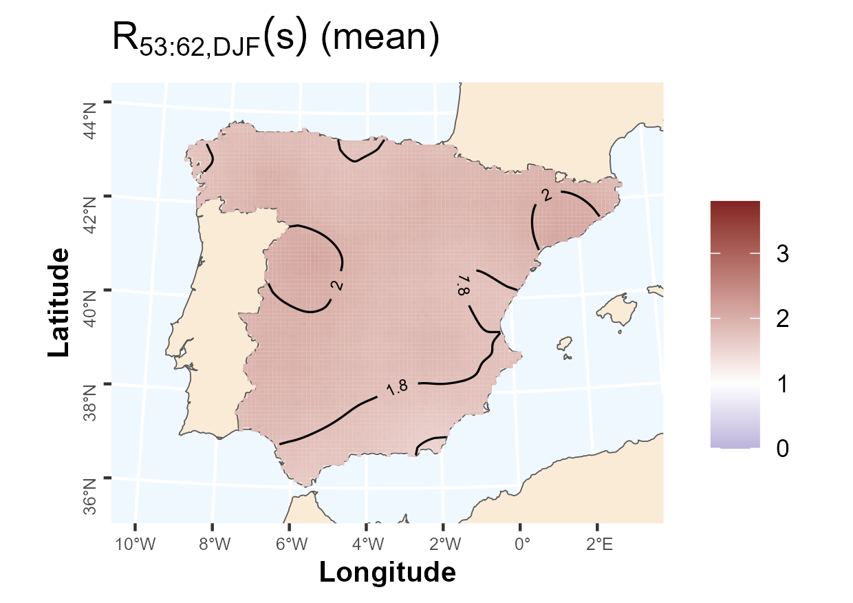
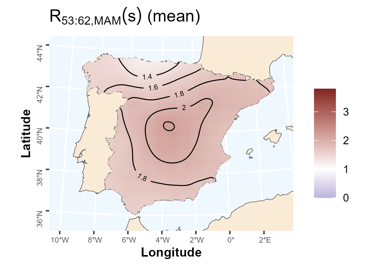
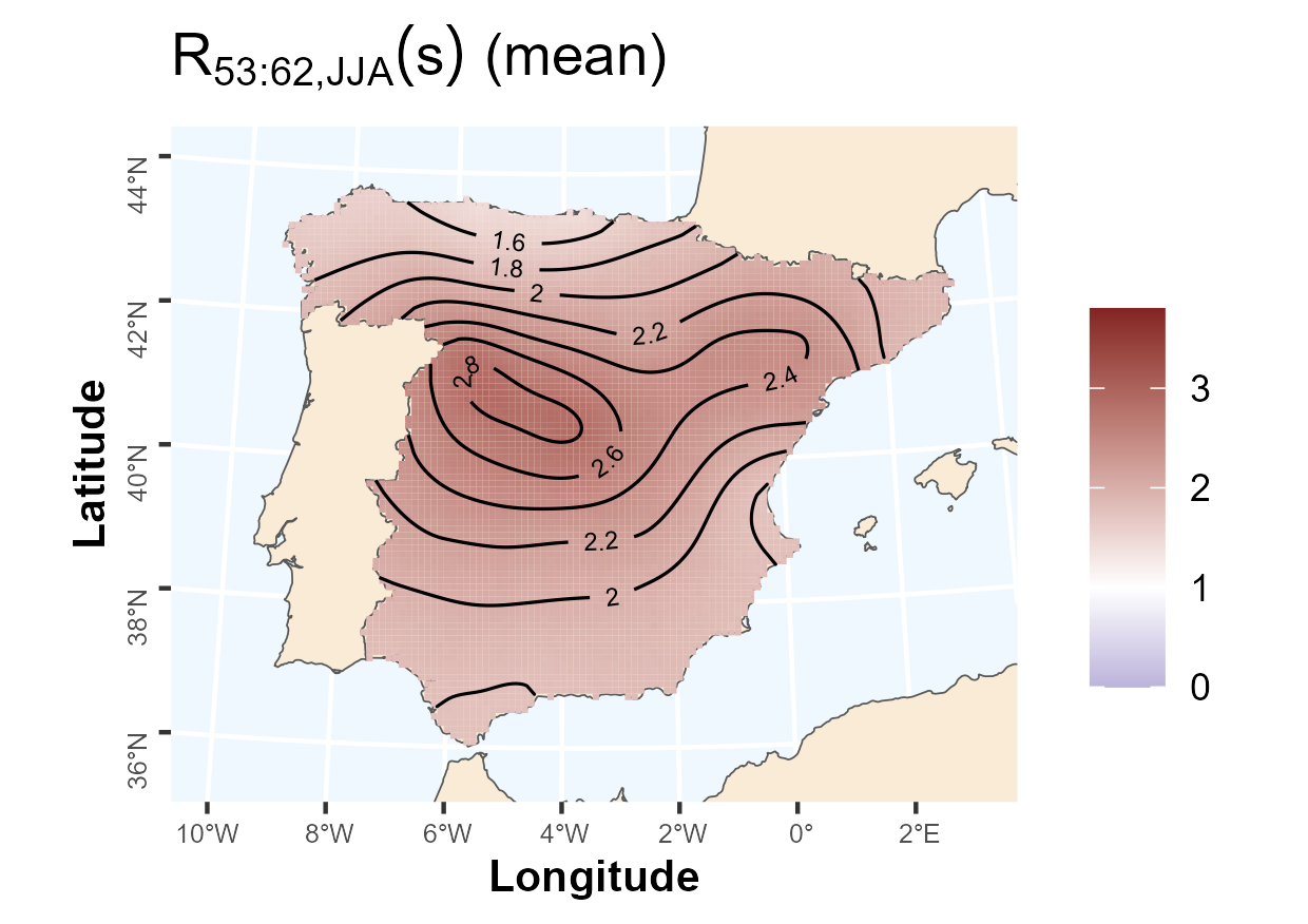
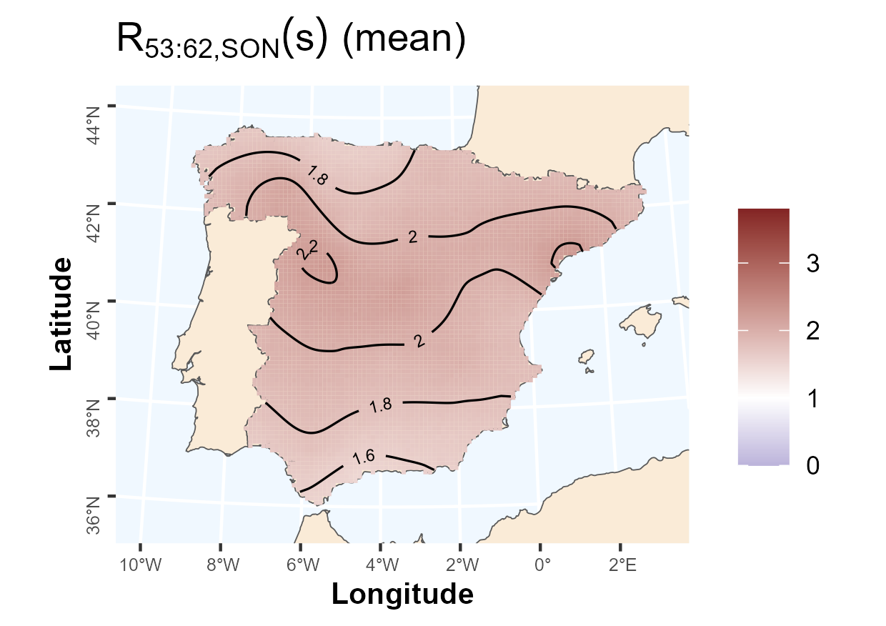
Figure 5: Map of the posterior mean of $R_{53:62,DJF}(\textbf{s})$ (winter, top–left), $R_{53:62,MAM}(\textbf{s})$ (spring, top–right), $R_{53:62,JJA}(\textbf{s})$ (summer, bottom–left), and $R_{53:62,SON}(\textbf{s})$ (autumn, bottom–right). Contour lines indicate ratios between intervals of length $0.2$.

Moving to annual evolution, Figure 6 shows the posterior mean and $90\%$ CI of $t\times\widehat{\overline{\text{ERS}}}_{t}(D)$ averaging in (4) against years. There is substantial variability across years, but with a clear approximately increasing linear trend from around $t=34$ (year 1993), which is not compatible with a stationary climate. The ERS has been consistently and clearly higher than 1 since $t=49$ (year 2008). This plot provides evidence of the strong effect that climate change has had on the occurrence of records in the 21st century, and particularly in the past decade. Specifically, the times $t=56$ and $t=58$ (years 2015 and 2017) exceeded the expected number of records under stationarity by more than two and a half times. Figure 14 of the Supplementary material repeats the same results by season showing that ERS is not homogeneous within years. The most relevant results show that in winter, the increase in the number of records is evident only during the last seven years. In contrast, in summer, deviations from stationarity start earlier and reach higher values; e.g., in summer 2003, the expected ERS under stationarity is multiplied by around $5$.

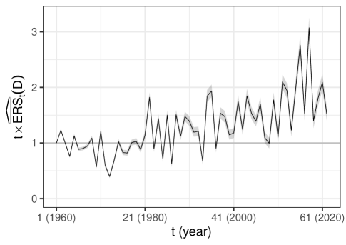
Figure 6: Posterior mean (black line) and $90\%$ CI (gray ribbon) of $t\times\widehat{\overline{\text{ERS}}}_{t}(D)$ against $t$. Expected value of $1$ under stationarity remarked for reference.

The model is also useful to obtain maps for the probability of record across days during a particular heatwave. To demonstrate the spatial and temporal extent of the August 14 ($\ell=225$), 2021 absolute record and August 2021 heatwave over peninsular Spain, Figure 7 shows the posterior mean of the probabilities of record $p_{62\ell}(\textbf{s})$ on days $\ell=222,\ldots,229$ within year 2021. This specific episode demonstrates the dynamics of persistence as well as the spatial structure of dependence. The beginning of the effects of the heatwave on the occurrence of records was observed on day 224, with posterior mean probabilities surpassing $0.5$ in the northeast. Over the following three days, the heatwave continued to evolve, with high probabilities observed across most regions, except for the coast, and with the area of high probabilities gradually diminished towards the southwest.

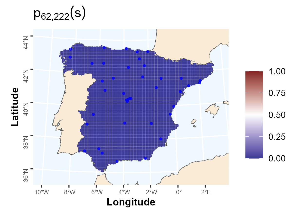
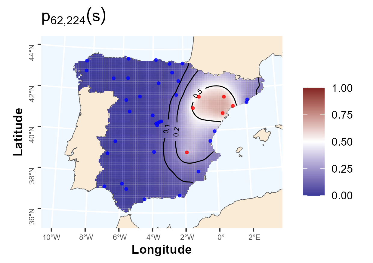
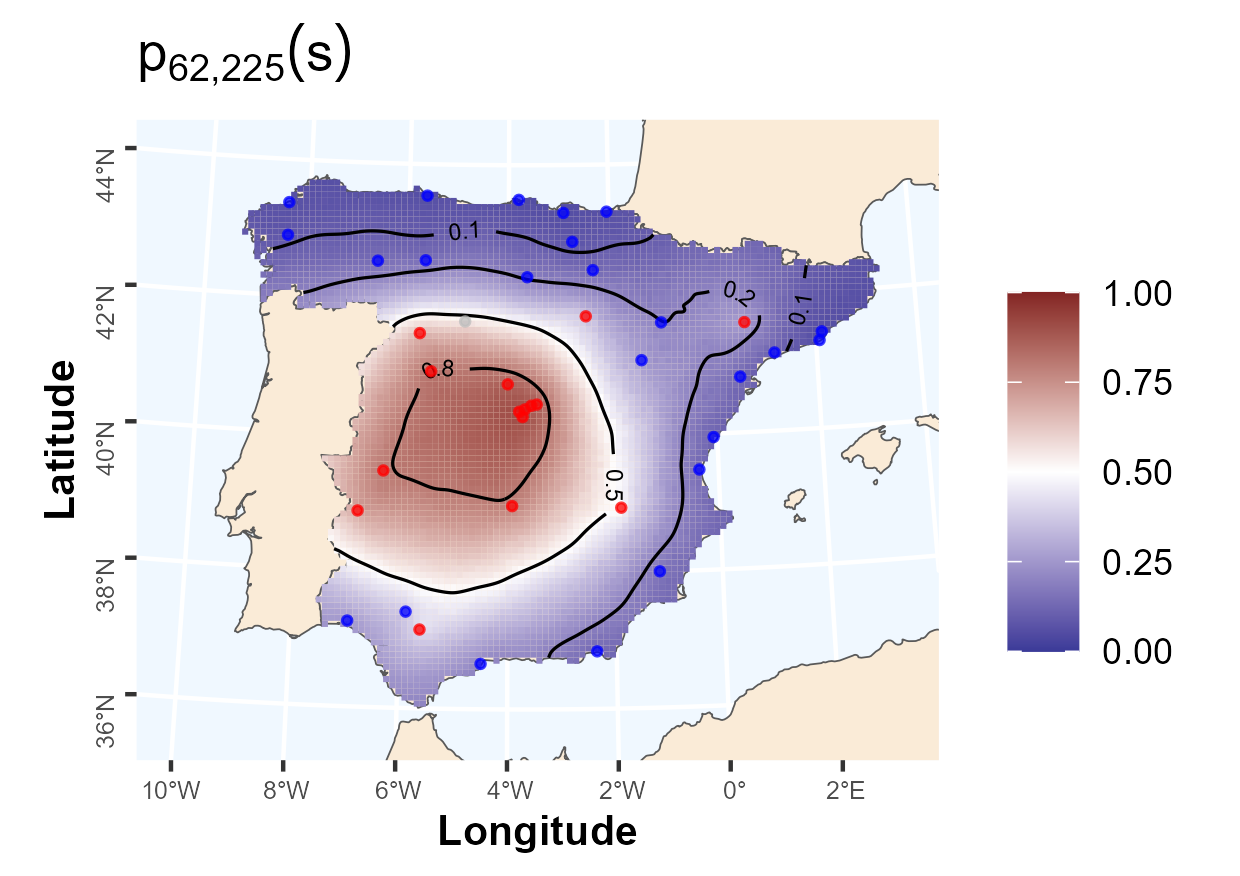
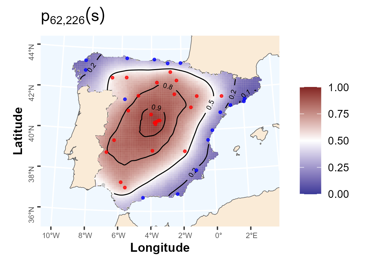
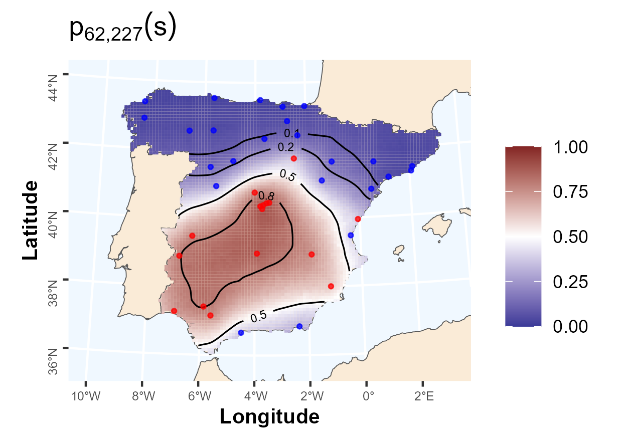
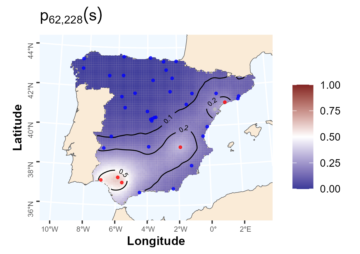
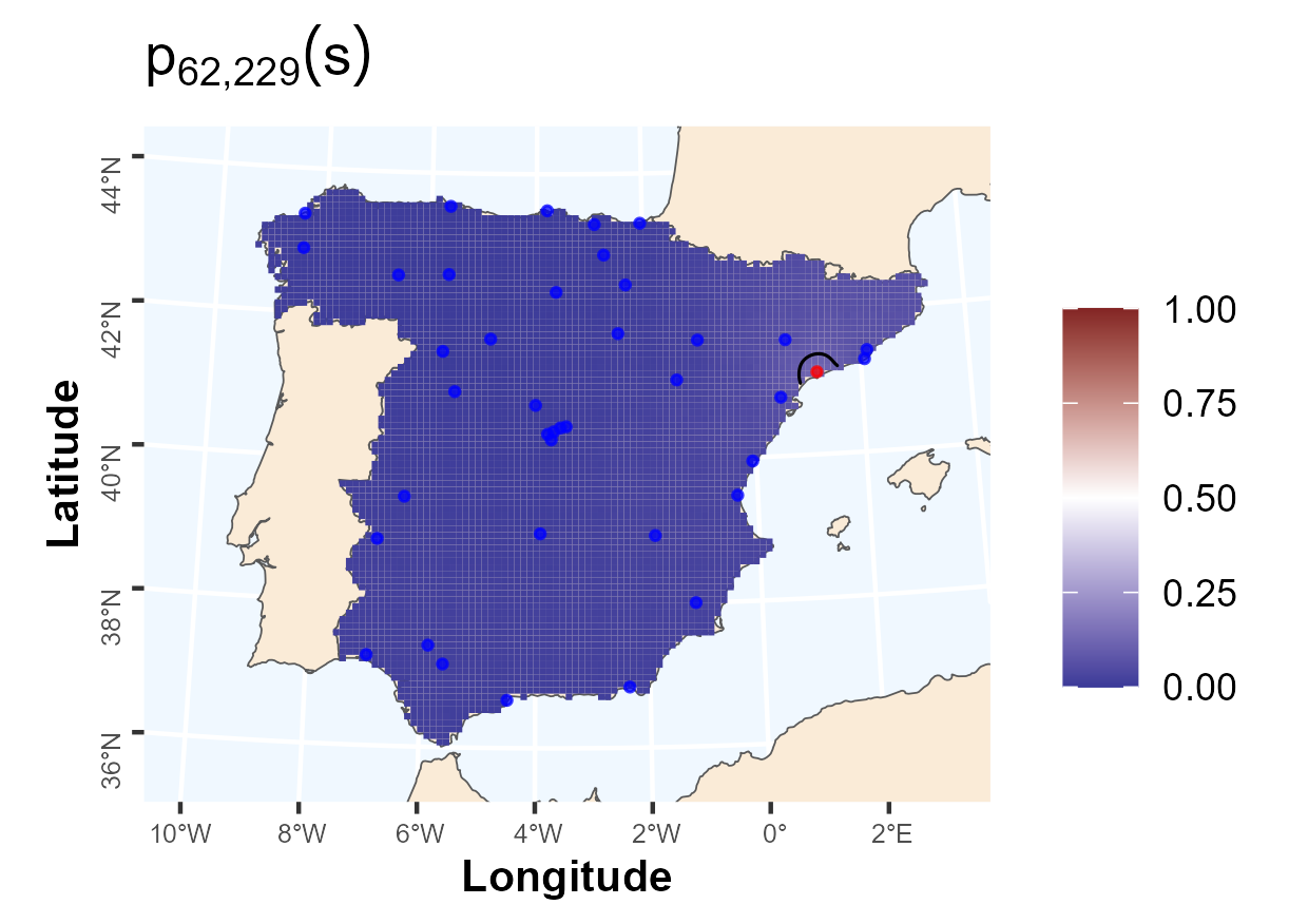
Figure 7: Maps of the posterior mean of $p_{62\ell}(\textbf{s})$ on days $\ell=222,\ldots,229$ within year 2021. Observed indicators are points in blue, gray, and red to indicate non-records, tied records, and records, respectively. Contour lines indicate probabilities $0.1$, $0.2$, $0.5$, $0.8$, $0.9$.

5 Summary and future work

Summary.

We have taken up the first fully developed modeling attempt to analyze the incidence of record-breaking temperatures. We have analyzed more than $60$ years of daily temperature data over peninsular Spain. The modeling needed to effectively explain the incidence of record-breaking over this region during this period required careful specification of the probabilities of the indicator functions which define record-breaking sequences. Key features include: explicit trend behavior, autoregression, significance of distance to the coast, useful interactions, spatial random effects, and very strong daily random effects.

Our main findings are that the pattern of occurrence of records over peninsular Spain during 1960–2021 is not compatible with stationary behavior of climate and that it accords with a global increase of temperature. More precisely, the total number of records in decade 2012–2021 has almost doubled compared to a stationary situation. In all the period from a spatial point of view, in $90.0\%$ of the region there is a significantly higher number of records compared to the stationary case, and there is no area where the number of records is significantly lower. Further, the increase in the number of records is not spatially homogeneous, being higher inland than coastal, and higher in the Mediterranean coast than in the Atlantic coast. The behavior is not homogeneous within year; during the past decade the highest increase has occurred in summer, and the lowest in spring.

Future work.

While we considered calendar day temperature records over peninsular Spain, the modeling proposed here can be useful for analyzing data from other parts of the world, other temporal scales, or for other climate signals such as ozone levels or rainfall.

There is interest in future incidence of record-breaking as a manifestation of future climate change. Such investigation will lead to analysis of future climate scenarios. Our approach here may prove useful though these scenarios are developed on spatial and temporal scales different from our current data, requiring substantial additional analysis. In particular, addressing this would require the inclusion of more information in the model, such as atmospheric covariates with future projections available or climate model simulations. Models that rely solely on time covariates for obtaining future projections may result in unsatisfactory extrapolation.

Another challenging problem with modeling calendar day records is that, for each day and location, we assume that the annual temperature series begins at the same year. With temperature data having initial year which varies with say space and day, it would be attractive not to discard many early years of indicator variables in order to achieve alignment in the dataset. One path for addressing varying record lengths could implement suitable posterior predictive “imputation” of the missing indicators at the sites having later initiation. Then, with replicates of the full series at each day at each site, the record breaking would be aligned and the predictive behavior could be explored. Such analysis does not arise with the dataset used here but presents a possible future investigation.

Supplementary material

Title:

Supplementary material Document with five sections: 1. Data and exploratory analysis, 2. Distributions for Gibbs sampling, 3. Model comparison and checking, 4. MCMC convergence diagnostics, 5. Additional results. (.pdf file)

R package:

R package sprom containing code to perform the spatial record occurrence modeling described in the manuscript. The package also contains a folder with data and a folder with R scripts to replicate the results in Section 4, including temperature data or covariates acquisition. (GNU zipped tar file)

Acknowledgments

This work was supported in part by MCIN/AEI/10.13039/501100011033 and Unión Europea NextGenerationEU under Grants PID2020-116873GB-I00 and TED2021-130702B-I00; and Gobierno de Aragón under Research Group E46_20R: Modelos Estocásticos. Jorge Castillo-Mateo was supported by Gobierno de Aragón under Doctoral Scholarship ORDEN CUS/581/2020 and Mobility Scholarship ORDEN CUS/1668/2022 number MVE_06_23. Zeus Gracia-Tabuenca was supported by Ministerio de Universidades and Unión Europea NextGenerationEU under Margarita Salas Scholarship RD 289/2021 UNI/551/2021. The authors thank Erin M. Schliep for useful discussions on Bayesian spatial binary regression and Jesús Abaurrea for valuable comments and insights.

Disclosure Statement

The authors report there are no competing interests to declare.

References

- (1)
- AEMET (2023) AEMET (2023), Informe sobre el estado del clima de España 2022, Technical report, Agencia Estatal de Meteorología, Madrid, Spain.
- Albert & Chib (1993) Albert, J. H. & Chib, S. (1993), ‘Bayesian analysis of binary and polychotomous response data’, Journal of the American Statistical Association 88(422), 669–679.
- Arnold et al. (1998) Arnold, B. C., Balakrishnan, N. & Nagaraja, H. N. (1998), Records, Wiley Series in Probability and Statistics, John Wiley & Sons, New York.
- Ballerini & Resnick (1985) Ballerini, R. & Resnick, S. (1985), ‘Records from improving populations’, Journal of Applied Probability 22(3), 487–502.
- Banerjee et al. (2014) Banerjee, S., Carlin, B. P. & Gelfand, A. E. (2014), Hierarchical Modeling and Analysis for Spatial Data, 2 edn, Chapman and Hall/CRC, New York, NY.
- Battisti & Naylor (2009) Battisti, D. S. & Naylor, R. L. (2009), ‘Historical warnings of future food insecurity with unprecedented seasonal heat’, Science 323(5911), 240–244.
- Benestad (2003) Benestad, R. E. (2003), ‘How often can we expect a record event?’, Climate Research 25(1), 3–13.
- Benestad (2004) Benestad, R. E. (2004), ‘Record-values, nonstationarity tests and extreme value distributions’, Global and Planetary Change 44(1–4), 11–26.
- Brier (1950) Brier, G. W. (1950), ‘Verification of forecasts expressed in terms of probability’, Monthly Weather Review 78(1), 1–3.
- C3S (2020) C3S (2020), European state of the climate 2019, Technical report, Copernicus Climate Change Service. Available at: https://climate.copernicus.eu/ESOTC/2019 (Accessed: December 10, 2023).
- Cardil et al. (2015) Cardil, A., Eastaugh, C. S. & Molina, D. M. (2015), ‘Extreme temperature conditions and wildland fires in Spain’, Theoretical and Applied Climatology 122(1), 219–228.
- Castillo-Mateo (2022) Castillo-Mateo, J. (2022), ‘Distribution-free changepoint detection tests based on the breaking of records’, Environmental and Ecological Statistics 29(3), 655–676.
- Castillo-Mateo, Asín, Cebrián, Gelfand & Abaurrea (2023) Castillo-Mateo, J., Asín, J., Cebrián, A. C., Gelfand, A. E. & Abaurrea, J. (2023), ‘Spatial quantile autoregression for season within year daily maximum temperature data’, Annals of Applied Statistics 17(3), 2305–2325.
- Castillo-Mateo, Cebrián & Asín (2023a) Castillo-Mateo, J., Cebrián, A. C. & Asín, J. (2023a), ‘RecordTest: An R package to analyse non-stationarity in the extremes based on record-breaking events.’, Journal of Statistical Software 106(5), 1–28.
- Castillo-Mateo, Cebrián & Asín (2023b) Castillo-Mateo, J., Cebrián, A. C. & Asín, J. (2023b), ‘Statistical analysis of extreme and record-breaking daily maximum temperatures in peninsular Spain during 1960–2021’, Atmospheric Research 293, 106934.
- Cebrián, Asín, Gelfand, Schliep, Castillo-Mateo, Beamonte & Abaurrea (2022) Cebrián, A. C., Asín, J., Gelfand, A. E., Schliep, E. M., Castillo-Mateo, J., Beamonte, M. A. & Abaurrea, J. (2022), ‘Spatio-temporal analysis of the extent of an extreme heat event’, Stochastic Environmental Research and Risk Assessment 36(9), 2737–2751.
- Cebrián, Castillo-Mateo & Asín (2022) Cebrián, A. C., Castillo-Mateo, J. & Asín, J. (2022), ‘Record tests to detect non-stationarity in the tails with an application to climate change’, Stochastic Environmental Research and Risk Assessment 36(2), 313–330.
- Chandler (1952) Chandler, K. N. (1952), ‘The distribution and frequency of record values’, Journal of the Royal Statistical Society: Series B (Methodological) 14(2), 220–228.
- Coumou et al. (2013) Coumou, D., Robinson, A. & Rahmstorf, S. (2013), ‘Global increase in record-breaking monthly-mean temperatures’, Climatic Change 118(3–4), 771–782.
- Czado et al. (2009) Czado, C., Gneiting, T. & Held, L. (2009), ‘Predictive model assessment for count data’, Biometrics 65(4), 1254–1261.
- Díaz-Poso et al. (2023) Díaz-Poso, A., Lorenzo, N. & Royé, D. (2023), ‘Spatio-temporal evolution of heat waves severity and expansion across the Iberian Peninsula and Balearic islands’, Environmental Research 217, 114864.
- Diggle et al. (1998) Diggle, P. J., Tawn, J. A. & Moyeed, R. A. (1998), ‘Model-based geostatistics’, Journal of the Royal Statistical Society: Series C (Applied Statistics) 47(3), 299–350.
- Elguindi et al. (2013) Elguindi, N., Rauscher, S. A. & Giorgi, F. (2013), ‘Historical and future changes in maximum and minimum temperature records over Europe’, Climatic Change 117, 415–431.
- Fischer et al. (2021) Fischer, E. M., Sippel, S. & Knutti, R. (2021), ‘Increasing probability of record-shattering climate extremes’, Nature Climate Change 11(8), 689–695.
- Franke et al. (2010) Franke, J., Wergen, G. & Krug, J. (2010), ‘Records and sequences of records from random variables with a linear trend’, Journal of Statistical Mechanics: Theory and Experiment 2010(10), P10013.
- Gouet et al. (2020) Gouet, R., Lafuente, M., López, F. J. & Sanz, G. (2020), ‘Exact and asymptotic properties of -records in the linear drift model’, Journal of Statistical Mechanics: Theory and Experiment 2020(10), 103201.
- Held & Holmes (2006) Held, L. & Holmes, C. C. (2006), ‘Bayesian auxiliary variable models for binary and multinomial regression’, Bayesian Analysis 1(1), 145–168.
- Klein Tank et al. (2002) Klein Tank, A. M. G., Wijngaard, J. B., Können, G. P., Böhm, R., Demarée, G., Gocheva, A., Mileta, M., Pashiardis, S., Hejkrlik, L., Kern-Hansen, C., Heino, R., Bessemoulin, P., Müller-Westermeier, G., Tzanakou, M., Szalai, S., Pálsdóttir, T., Fitzgerald, D., Rubin, S., Capaldo, M., Maugeri, M., Leitass, A., Bukantis, A., Aberfeld, R., van Engelen, A. F. V., Forland, E., Mietus, M., Coelho, F., Mares, C., Razuvaev, V., Nieplova, E., Cegnar, T., Antonio López, J., Dahlström, B., Moberg, A., Kirchhofer, W., Ceylan, A., Pachaliuk, O., Alexander, L. V. & Petrovic, P. (2002), ‘Daily dataset of 20th-century surface air temperature and precipitation series for the European Climate Assessment’, International Journal of Climatology 22(12), 1441–1453.
- Linares Gil et al. (2017) Linares Gil, C., Carmona Alférez, R., Ortiz Burgos, C. & Díaz Jiménez, J. (2017), Temperaturas extremas y salud: Cómo nos afectan las olas de calor y de frío, Catarata, Madrid, España.
- Lionello & Scarascia (2018) Lionello, P. & Scarascia, L. (2018), ‘The relation between climate change in the Mediterranean region and global warming’, Regional Environmental Change 18, 1481–1493.
- McBride et al. (2022) McBride, C. M., Kruger, A. C. & Dyson, L. (2022), ‘Trends in probabilities of temperature records in the non-stationary climate of South Africa’, International Journal of Climatology 42(3), 1692–1705.
- NOAA (2023) NOAA (2023), ‘Data tools: Daily weather records’. Available at: https://www.ncdc.noaa.gov/cdo-web/datatools/records (Accessed: December 10, 2023).
- Pan et al. (2013) Pan, Z., Wan, B. & Gao, Z. (2013), ‘Asymmetric and heterogeneous frequency of high and low record-breaking temperatures in China as an indication of warming climate becoming more extreme’, Journal of Geophysical Research: Atmospheres 118(12), 6152–6164.
- Plumer & Shao (2023) Plumer, B. & Shao, E. (2023), ‘Heat records are broken around the globe as Earth warms, fast’, The New York Times . Available at: https://www.nytimes.com/2023/07/06/climate/climate-change-record-heat.html (Accessed: July 9, 2023).
- Polson et al. (2013) Polson, N. G., Scott, J. G. & Windle, J. (2013), ‘Bayesian inference for logistic models using Pólya–gamma latent variables’, Journal of the American Statistical Association 108(504), 1339–1349.
- Rahmstorf & Coumou (2011) Rahmstorf, S. & Coumou, D. (2011), ‘Increase of extreme events in a warming world’, Proceedings of the National Academy of Sciences 108(44), 17905–17909.
- Robin et al. (2011) Robin, X., Turck, N., Hainard, A., Tiberti, N., Lisacek, F., Sanchez, J.-C. & Müller, M. (2011), ‘pROC: an open-source package for R and S+ to analyze and compare ROC curves’, BMC Bioinformatics 12, 77.
- Sillmann et al. (2017) Sillmann, J., Thorarinsdottir, T., Keenlyside, N., Schaller, N., Alexander, L. V., Hegerl, G., Seneviratne, S. I., Vautard, R., Zhang, X. & Zwiers, F. W. (2017), ‘Understanding, modeling and predicting weather and climate extremes: Challenges and opportunities’, Weather and Climate Extremes 18, 65–74.
- Sousa et al. (2019) Sousa, P. M., Barriopedro, D., Ramos, A. M., García-Herrera, R., Espírito-Santo, F. & Trigo, R. M. (2019), ‘Saharan air intrusions as a relevant mechanism for Iberian heatwaves: The record breaking events of August 2018 and June 2019’, Weather and Climate Extremes 26, 100224.
- Spiegelhalter et al. (2002) Spiegelhalter, D. J., Best, N. G., Carlin, B. P. & Van Der Linde, A. (2002), ‘Bayesian measures of model complexity and fit’, Journal of the Royal Statistical Society: Series B (Statistical Methodology) 64(4), 583–639.
- Wergen et al. (2014) Wergen, G., Hense, A. & Krug, J. (2014), ‘Record occurrence and record values in daily and monthly temperatures’, Climate Dynamics 42(5), 1275–1289.
- WMO (2022) WMO (2022), State of the Global Climate 2021, Technical Report WMO-No. 1290, WMO, Geneva, Switzerland.