ab
\usephysicsmoduleop.legacy
\usephysicsmodulebraket
\usephysicsmodulenabla.legacy
High-purity single-photon generation based on cavity QED
Seigo Kikura
kikura@qi.t.u-tokyo.ac.jpDepartment of Applied Physics, Graduate School of Engineering, The University of Tokyo, 7-3-1 Hongo, Bunkyo-ku, Tokyo 113-8656, Japan
Rui Asaoka
Computer and Data Science Laboratories, NTT Corporation, Musashino 180-8585, Japan
Masato Koashi
Department of Applied Physics, Graduate School of Engineering, The University of Tokyo, 7-3-1 Hongo, Bunkyo-ku, Tokyo 113-8656, Japan
Photon Science Center, Graduate School of Engineering, The University of Tokyo, 7-3-1 Hongo, Bunkyo-ku, Tokyo 113-8656, Japan
Yuuki Tokunaga
Computer and Data Science Laboratories, NTT Corporation, Musashino 180-8585, Japan
Abstract
We propose a scheme for generating a high-purity single photon on the basis of cavity quantum electrodynamics (QED).
This scheme employs a four-level system including two excited states, two ground states, and two driving lasers; this structure allows the suppression of the re-excitation process due to the atomic decay, which is known to significantly degrade the single-photon purity in state-of-the-art photon sources using a three-level system.
Our analysis shows that the re-excitation probability arbitrarily approaches zero without sacrificing the photon generation probability when increasing the power of the driving laser between the excited states.
This advantage is achievable by using current cavity-QED technologies.
Our scheme can contribute to developing distributed quantum computation or quantum communication with high accuracy.
Single-photon sources based on cavity quantum electrodynamics (QED) are of paramount importance for quantum information processing that ranges from quantum computation [1, 2] and quantum communication [3, 4].
Notably, photon sources using a -type three-level atom have the advantage of controlling the temporal mode of an emitted photon, have been well studied for their performance [5, 6, 7, 8, 9], and have been demonstrated in several practical applications [10, 11, 12, 13, 14, 15, 16, 17].
In photonic quantum information science, various protocols harness quantum interference of photons, where photon sources should preferably generate high-purity single photons.
In the three-level photon generation scheme, however, the atomic spontaneous decay and following re-excitation reduce the purity of photons.
In fact, several recent experiments have reported that the re-excitation significantly deteriorates the Hong-Ou-Mandel interference visibility [14, 18, 15].
Although choosing an appropriate initial state or truncating the generation process has been proposed to tackle this problem [15, 11], these strategies have limitations in improving the purity, and especially the latter also sacrifices the total photon generation probability.
Here we propose a scheme for generating a high-purity single photon on the basis of cavity QED.
This scheme employs a four-level system including two excited states, two ground states, and two driving lasers.
Using an additional energy level to suppress atomic decay has been examined in some protocols [19, 20, 21, 22].
In our protocol, this strategy is developed to generate a high-purity photon on the basis of cavity QED.
To evaluate the performance of our scheme, we analyze the four-level system proposed here by using the effective operator formalism [23], which shows that the re-excitation probability is greatly inhibited in our scheme compared to in the previous three-level one.
The distinct advantage of our scheme is that the photon generation probability is hardly sacrificed.
Finally, we propose a realistic implementation of our scheme using only optical transitions.
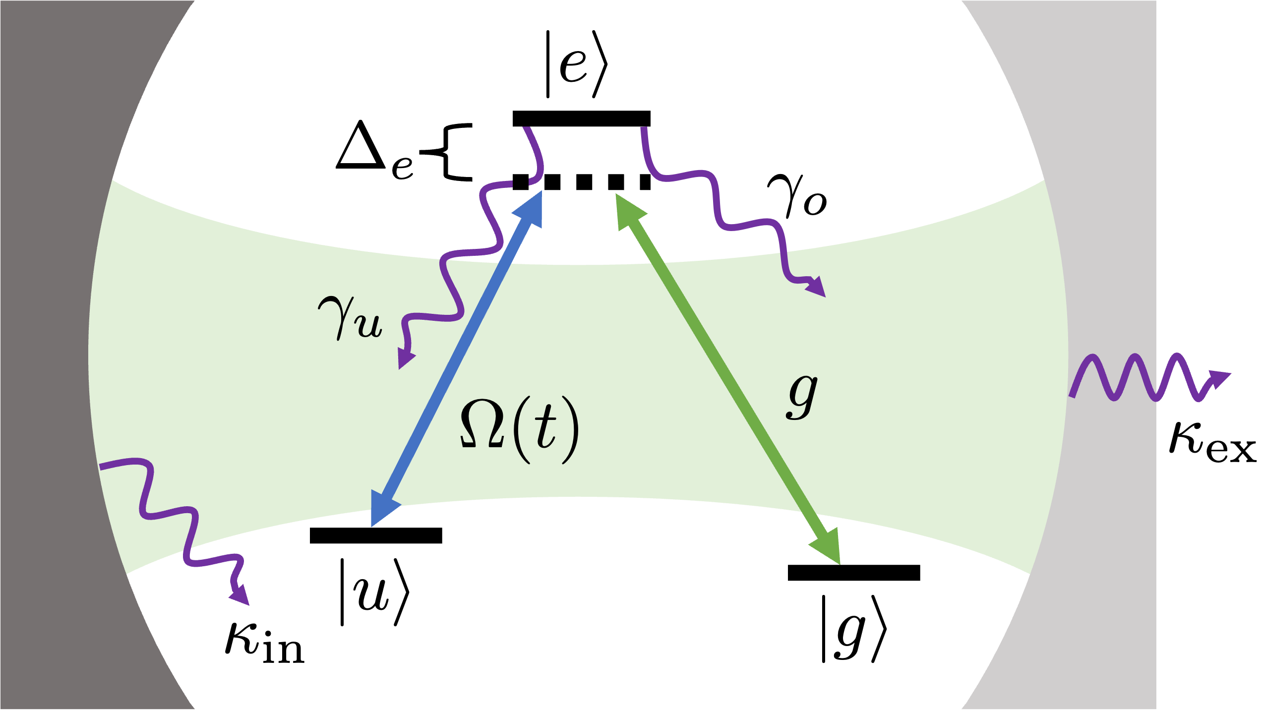
Figure 1: Three-level system and a cavity for single-photon generation
We first analyze a -type three-level atom in a one-sided cavity shown in Fig. 1 to compare our method with the conventional one that uses this system.
The system is formed by two metastable levels , and one excited level .
The transition is driven by an external driving pulse of frequency with Rabi frequency .
The transition is coupled to a cavity mode of frequency with coupling strength , which is defined as a real number.
The Hamiltonian in a proper rotating frame is
(1)
where , is the annihilation (creation) operator for the cavity mode, is a frequency for the energy of , and we set .
This Hamiltonian couples only three states , where the number represents the photon number of the cavity mode.
When the system is initially prepared in , we can thus use a simplified Hamiltonian in the manifold
(2)
where we define and assume .
We describe the cavity decay and atomic spontaneous decay with Lindblad operators:
corresponds to the cavity decay where a photon is emitted into the desired external mode, corresponds to the cavity decay including scattering into undesired modes and intracavity losses, and corresponds to the atomic decay from to .
We use an operator to represent atomic decays from to levels outside the manifold .
Those levels may include and other atomic levels except and .
Without loss of generality, we treat it as a decay to a single level and assume that .
We define as the total cavity loss rate and as the total rate of spontaneous decay.
The master equation describes the time evolution of this atom-cavity system as
(3)
where .
The quantum jumps and lead to the failure of the photon generation, whereas the quantum jump leads to the success.
The quantum jump initializes the system and then the photon generation process re-starts.
We call a process where the decay does not occur a single excitation and a process where the decay occurs even just once a re-excitation process.
We assume that the intensity and time variation of the driving pulse are small.
This assumption, which has been used in many previous works [24, 9, 8, 17], enables us to use the effective operator formalism [23].
This formalism shows that a state in an excited subspace is with , and describes the time evolution of ground states as a master equation with effective Hamiltonian and Lindblad operators
as follows [25]:
(4)
(5)
(6)
By using the effective operators, we determine the final state of the desired mode in the following way.
We classify the single-photon emission events using a label , which is a non-negative number: In the event with , no quantum jumps occur during and a jump occurs at , where is arbitrary.
For , the event refers to the case where a jump occurs at , no quantum jumps occur during , and a jump occurs at , where is arbitrary.
Those events and the complement (no photon emission) are mutually exclusive and are also
distinguishable without looking at the desired mode in principle because the occurrence and its time of a quantum jump () can be recorded in the
associated environment.
Hence the final state of the desired mode is given by
a mixture of those events as
(7)
where is a vacuum state of the desired mode.
Here is the rate of quantum jump at , which is to be determined from the effective master equation.
The unnormalized state vector represents the state of the emitted single photon with no quantum jumps during except the jump , on condition that the atom-cavity system is in state at time .
These are pure states because the events involve only quantum jumps whose environment is the desired mode.
In fact, the state is related to the time evolution of
the atom-cavity system as
(8)
where is the output field operator.
Here is the state of the atom-cavity system at time with no quantum jumps during , on condition that it is in state at time .
More precisely, the normalized solution of the effective master equation with is written in the form with representing an unnormalized state after one or more quantum jumps.
The time dependence of state is determined by solving
(9)
with initial condition .
The first and second terms on the right-hand side of the Eq. (7) respectively correspond to the single-photon states emitted by single and re-excitation processes.
The probability of the photon generation up to time for the single(re-) excitation process is calculated as
(10)
(11)
where
We assume that we apply for a sufficiently long time so that the population of finally becomes zero.
In this case, the photon generation probabilities of the single excitation and total processes are given by
(12)
(13)
The ratio of the photon produced by the re-excitation process is .
Equations (12) and (13) agree with the universal upper bound for photon generation in a -type three-level system [5].
The quality of a single-photon source may be evaluated by using several quantities.
One is the efficiency of producing a photon, which has already appeared in the above derivation.
To further evaluate the quality of the temporal modes of the single photon, we assume that the state of the emitted light is written by
(14)
and define single-photon purity and single-photon fidelity by
(15)
This purity relates to the Hong-Ou-Mandel interference visibility [26].
Substituting Eq. (7) gives these two measures as [25]
(16)
Therefore, the performance depends only on the total photon generation probability and the ratio of the re-excitation process, rather than the driving pulse.
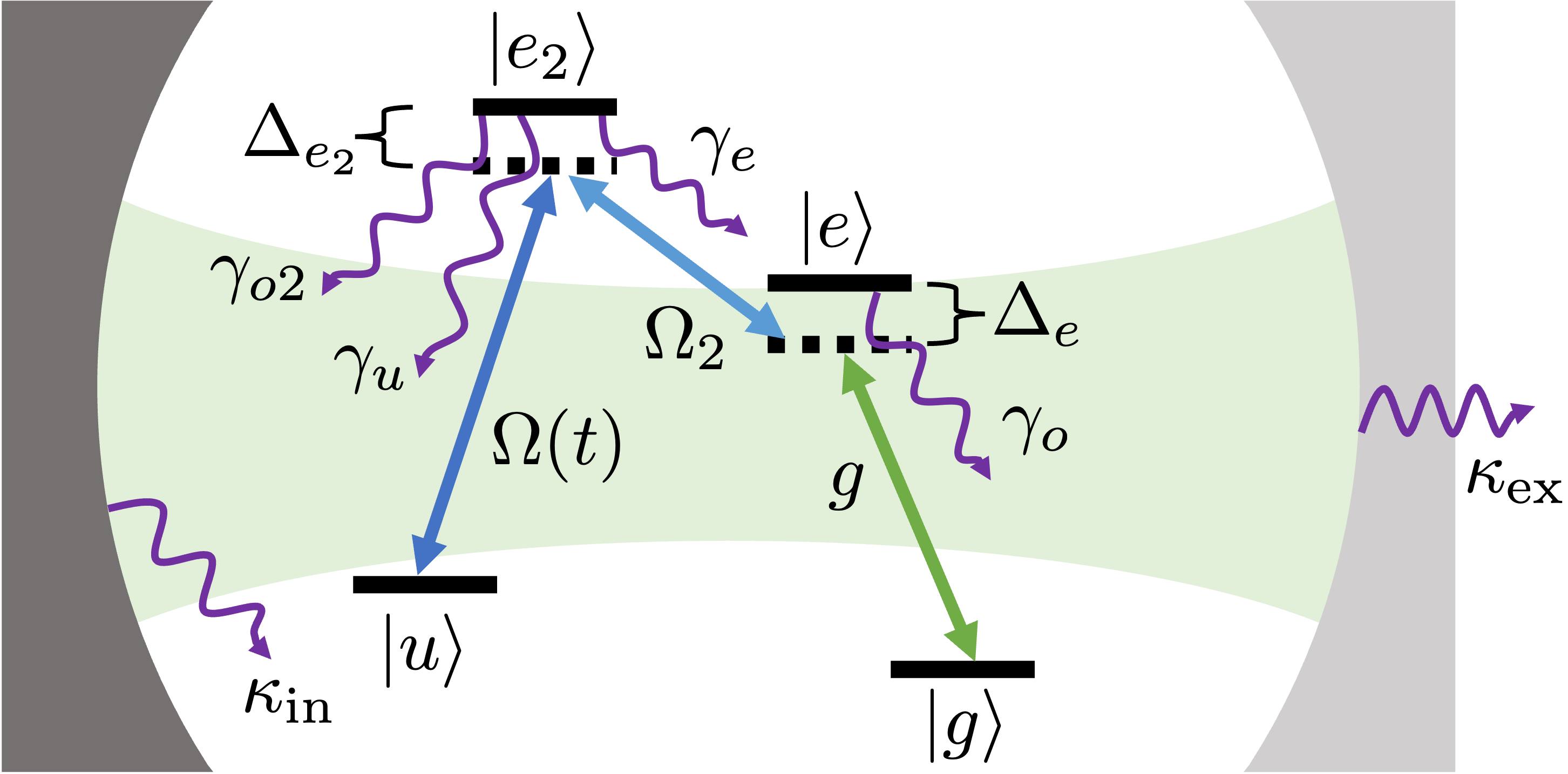
Figure 2: Four-level system and a cavity
The above discussion indicates that the total photon generation probability needs to be improved and the re-excitation process suppressed to improve the performance of the single-photon source.
Equations (12) and (13) show that both goals can be achieved by increasing .
This improvement, however, requires an experimental breakthrough, and thus other methods to improve the performance need to be proposed.
To suppress the re-excitation, we propose a four-level system where we add an excited level , shown in Fig. 2.
The transition is driven by the driving pulse and transition is driven by an additional laser of frequency with Rabi frequency , which is defined as a real constant.
We define and as the decay rates from to and to , where we represent atomic decay to levels other than , and by decay to a single level .
We assume that the decay is prohibited by a selection rule.
In the three-level system, the fact that the state vector of excited states is leads to increasing reducing the population of during the photon generation process and thus suppresses the re-excitation process.
In the four-level system, increasing , which can be easily controlled, will reduce the population of and thus lead to suppression.
To confirm this expectation, we now analyze the four-level system in the same way we did the three-level one.
The Hamiltonian describing the four-level system in a proper rotating frame is given as
(17)
where we define as the frequency for the energy of , , and assume .
Here we assume to compare the four-level system with the three-level one.
We will later discuss the case with and show that these decays will not be an additional problem.
Lindblad operators are given as , and .
When assuming the intensity and time variation of the driving pulse are small, we can use the effective operator formalism and find that a state in an excited subspace is with .
Thus, we can decrease the population of by setting and increasing , suppressing the re-excitation process.
We demonstrate that the total photon generation probability is consistent with Eq. (13) whereas the ratio of the re-excitation process is
(18)
and Eqs. (16) hold by replacing [25].
This ratio is minimized for and is made to further approach zero by increasing such that .
This result shows that means .
Thus, even without increasing , increasing suppresses the re-excitation process while maintaining the total photon generation probability.
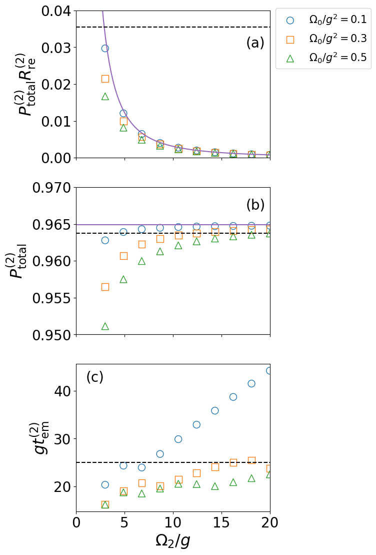
Figure 3: Photon generation probability and emission time as a function of . All detunings of the three- and four-level systems are zero and and , which maximizes [5].
Dashed lines show the result of the three-level system that includes the minimum emission time when optimizing and the corresponding photon generation probability.
The optimal value is .
Solid lines show the analytical result.
We calculate the photon generation probability and an emission time by numerically solving the master equation (3), where we use a QuTiP 2 package [27].
In this calculation, we assume the driving pulse that has a linear shape, i.e., .
The symbols in Figs. 3(a) and 3(b) show the photon generation probability for the re-excitation process and the total probability with the analytical values represented by the solid lines.
These simulations show that the smaller is, the smaller the deviation between exact solutions and ones by the effective operator formalism is.
These numerical results demonstrate that setting small and increasing such that suppresses the re-excitation process without diminishing the total photon generation probability compared to the three-level system.
Figure 3(c) shows an emission time by numerical calculation.
Here we define a photon emission time of the four-level system as a time when the photon generation probability for the single excitation process becomes 0.99 of its maximum value, i.e. .
We can find that the photon emission time increases when increases.
This behavior can be explained analytically.
We can find that the generation probability up to time for the single excitation process is given as , where we define [25].
This equation indicates that for a given shape of , increasing makes small.
We can derive the upper bound of as whose equality holds when
(19)
This inequality thus shows a trade-off between the photon emission time and the ratio of the re-excitation process.
Note that the trade-off is also valid for the three-level system.
However, the numerical result shows that increasing suppresses the delay of photon generation with a slight sacrifice of .
So far, we have assumed , but there may be non-negligible decay in real atoms.
The former decay does not decrease the single-photon purity and fidelity but the total photon generation probability, whereas the latter decay affects all of them.
However, we can neglect both decays in the limit because our system can decrease the population of and suppress all decays from by increasing [25].
To realize our scheme, we need to use an atom that satisfies two following requirements:
The decay is prohibited by the selection rule.
The large can be applied.
For example, satisfies these reqirements by defining the states of interest as , and .
All optical transitions between these states and the coupling with a cavity field have been realized experimentally [28, 29, 30].
In conclusion, we have introduced a scheme for generating a high-purity photon on the basis of cavity QED.
This scheme can reduce the probability of the re-excitation process close to zero, without sacrificing the total photon generation probability, by increasing the driving-laser power between the excited states.
Our scheme may increase the difficulty of experiments, but we have proposed a specific implementation using , where all optical transitions and the coupling with a cavity have been realized experimentally.
Thus, our proposal is implementable with the current cavity-QED technologies.
We thank Hiroki Takahashi, Akihisa Goban, and Shinichi Sunami for their advice.
This research was supported by JST (Moonshot R&D)(Grant No. JPMJMS2061).
References
Knill et al. [2001]E. Knill, R. Laflamme, and G. J. Milburn, A scheme for efficient quantum computation with linear optics, Nature 409, 46 (2001).
Monroe et al. [2014]C. Monroe, R. Raussendorf, A. Ruthven, K. R. Brown, P. Maunz, L.-M. Duan, and J. Kim, Large-scale modular quantum-computer architecture with atomic memory and photonic interconnects, Phys. Rev. A 89, 022317 (2014).
Kimble [2008]H. J. Kimble, The quantum internet, Nature 453, 1023 (2008).
Covey et al. [2023]J. P. Covey, H. Weinfurter, and H. Bernien, Quantum networks with neutral atom processing nodes, npj Quantum Information 9, 10.1038/s41534-023-00759-9 (2023).
Goto et al. [2019]H. Goto, S. Mizukami, Y. Tokunaga, and T. Aoki, Figure of merit for single-photon generation based on cavity quantum electrodynamics, Phys. Rev. A 99, 053843 (2019).
Utsugi et al. [2022]T. Utsugi, A. Goban, Y. Tokunaga, H. Goto, and T. Aoki, Gaussian-wave-packet model for single-photon generation based on cavity quantum electrodynamics under adiabatic and nonadiabatic conditions, Phys. Rev. A 106, 023712 (2022).
Giannelli et al. [2018]L. Giannelli, T. Schmit, T. Calarco, C. P. Koch, S. Ritter, and G. Morigi, Optimal storage of a single photon by a single intra-cavity atom, New Journal of Physics 20, 105009 (2018).
Gorshkov et al. [2007]A. V. Gorshkov, A. André, M. D. Lukin, and A. S. Sørensen, Photon storage in -type optically dense atomic media. i. cavity model, Phys. Rev. A 76, 033804 (2007).
Keller et al. [2004]M. Keller, B. Lange, K. Hayasaka, W. Lange, and H. Walther, Continuous generation of single photons with controlled waveform in an ion-trap cavity system, NATURE 431, 1075 (2004).
Barros et al. [2009]H. G. Barros, A. Stute, T. E. Northup, C. Russo, P. O. Schmidt, and R. Blatt, Deterministic single-photon source from a single ion, New Journal of Physics 11, 103004 (2009).
Nisbet-Jones et al. [2011]P. B. R. Nisbet-Jones, J. Dilley, D. Ljunggren, and A. Kuhn, Highly efficient source for indistinguishable single photons of controlled shape, New Journal of Physics 13, 103036 (2011).
Meraner et al. [2020]M. Meraner, A. Mazloom, V. Krutyanskiy, V. Krcmarsky, J. Schupp, D. A. Fioretto, P. Sekatski, T. E. Northup, N. Sangouard, and B. P. Lanyon, Indistinguishable photons from a trapped-ion quantum network node, Phys. Rev. A 102, 052614 (2020).
Walker et al. [2020]T. Walker, S. V. Kashanian, T. Ward, and M. Keller, Improving the indistinguishability of single photons from an ion-cavity system, Phys. Rev. A 102, 032616 (2020).
Schupp et al. [2021]J. Schupp, V. Krcmarsky, V. Krutyanskiy, M. Meraner, T. Northup, and B. Lanyon, Interface between trapped-ion qubits and traveling photons with close-to-optimal efficiency, PRX Quantum 2, 020331 (2021).
Morin et al. [2019]O. Morin, M. Körber, S. Langenfeld, and G. Rempe, Deterministic shaping and reshaping of single-photon temporal wave functions, Phys. Rev. Lett. 123, 133602 (2019).
Krutyanskiy et al. [2023]V. Krutyanskiy, M. Galli, V. Krcmarsky, S. Baier, D. A. Fioretto, Y. Pu, A. Mazloom, P. Sekatski, M. Canteri, M. Teller, J. Schupp, J. Bate, M. Meraner, N. Sangouard, B. P. Lanyon, and T. E. Northup, Entanglement of trapped-ion qubits separated by 230 meters, Phys. Rev. Lett. 130, 050803 (2023).
Porras and Cirac [2008]D. Porras and J. I. Cirac, Collective generation of quantum states of light by entangled atoms, Phys. Rev. A 78, 053816 (2008).
Borregaard et al. [2015]J. Borregaard, P. Kómár, E. M. Kessler, A. S. Sørensen, and M. D. Lukin, Heralded quantum gates with integrated error detection in optical cavities, Phys. Rev. Lett. 114, 110502 (2015).
González-Tudela et al. [2017]A. González-Tudela, V. Paulisch, H. J. Kimble, and J. I. Cirac, Efficient multiphoton generation in waveguide quantum electrodynamics, Phys. Rev. Lett. 118, 213601 (2017).
Paulisch et al. [2018]V. Paulisch, H. J. Kimble, J. I. Cirac, and A. González-Tudela, Generation of single- and two-mode multiphoton states in waveguide qed, Phys. Rev. A 97, 053831 (2018).
Reiter and Sørensen [2012]F. Reiter and A. S. Sørensen, Effective operator formalism for open quantum systems, Phys. Rev. A 85, 032111 (2012).
Beloy et al. [2012]K. Beloy, J. A. Sherman, N. D. Lemke, N. Hinkley, C. W. Oates, and A. D. Ludlow, Determination of the state lifetime and blackbody-radiation clock shift in yb, Phys. Rev. A 86, 051404 (2012).
Saskin et al. [2019]S. Saskin, J. T. Wilson, B. Grinkemeyer, and J. D. Thompson, Narrow-line cooling and imaging of ytterbium atoms in an optical tweezer array, Phys. Rev. Lett. 122, 143002 (2019).
Pedrozo-Peñafiel et al. [2020]E. Pedrozo-Peñafiel, S. Colombo, C. Shu, A. F. Adiyatullin, Z. Li, E. Mendez, B. Braverman, A. Kawasaki, D. Akamatsu, Y. Xiao, and V. Vuletić, Entanglement on an optical atomic-clock transition, Nature 588, 414–418 (2020).
Supplementary Material for “High-purity single-photon generation based on cavity QED”
S1 Effective operator formalism
We will summarize the effective operator formalism proposed by Reiter and Sørensen [23].
We consider an open system that consists of two distinct subspaces: ground subspace and decaying excited subspace.
We define and as projection operators onto ground subspace and decaying excited subspace and decompose the Hamiltonian as follows:
(S1)
We assume that and the coupling of these two subspaces are perturbative.
We then approximate
(S2)
and find that a state in the excited subspace is given by
(S3)
where we define a non-Hermitian Hamiltonian as
(S4)
and .
Accordingly, the dynamics of a state in ground subspace is governed by
(S5)
with effective Hamiltonian and Lindblad operators
(S6)
(S7)
We will now extend the original results to consider the case with time-dependent couplings .
By assuming that the time variation of is small in the time scale set by , we find
(S8)
Accordingly, we straightforwardly extend the derivation in Reiter and Sørensen [23],
and the state in the excited subspace is given by
(S9)
We also obtain the effective master equation as
(S10)
with effective Hamiltonian and Lindblad operators
(S11)
(S12)
We apply this extended effective master equation to three- and four-level systems in the following.
Three-level system
We analyze the -type three-level system as shown in Fig. 1 in the article.
The Hamiltonian is given by Eq. (2) in the article and is reproduced here
To ease the following notation, we define the effective detuning and decay rates as follows:
(S21)
(S22)
(S23)
(S24)
We first derive the state of the atom-cavity system at time with no quantum jumps during , on condition that it is in state at time .
The time dependence of state is determined by solving
(S25)
with initial condition .
We can find that
(S26)
and
(S27)
Equations (S18) and (S27) give the emitted single-photon state as
(S28)
(S29)
Second, we derive the rate of quantum jump at .
From Eq. (S10), we derive the differential equation for the population of as
(S30)
where .
With the initial condition , this equation gives
(S31)
We then derive the rate as follows:
(S32)
We can find the probability of the photon generation from those values.
The probability of the photon generation up to time for the single(re-) excitation process is given as follows:
(S33)
(S34)
When applying for a sufficiently long time so that the population of finally becomes zero, the photon generation probabilities of the single excitation and total processes are given as follows:
We analyze the four-level system as shown in Fig. 2 in the article.
We assume to compare the four-level system with the three-level one.
The Hamiltonian is given by Eq. (17) in the article and is reproduced here
(S39)
(S40)
(S41)
By assuming the intensity and time variation of , we can follow the same recipe as before and derive the state in the excited subspace as
(S42)
and the effective operators as follows:
(S43)
(S44)
(S45)
(S46)
where we define
(S47)
We then define the effective detuning and decay rates as follows:
(S48)
(S49)
(S50)
(S51)
(S52)
From the effective operators, we find the probability of the photon generation up to time for the single(re-) excitation process as follows:
(S53)
(S54)
When applying for a sufficiently long time so that the population of finally becomes zero, the photon generation probabilities of the single excitation and total processes are given as follows:
(S55)
(S56)
We can also find the ratio of the re-excitation process as
We use single-photon purity and fidelity as performance measures of a single-photon source.
We first consider the three-level system.
The purity and fidelity are given by
When considering the four-level system, we can also derive these measures as before:
(S70)
These results show that these measures depend only on the ratio of the re-excitation process, rather than .
Case with
So far, we have assumed . We now remove this assumption and analyze these effects.
Our following analytical analysis shows that we can neglect the effect of and in the limit .
We first consider the case with .
We can describe the decay by a Lindblad operator .
By using the effective operator formalism, we can find the corresponding effective Lindblad operator as
(S71)
and derive the total photon probability and the ratio of the re-excitation process by replacing
(S72)
(S73)
where we define
(S74)
We can find is minimized for , and in this case in the limit .
We further consider the case with .
We can describe the decay by a Lindblad operator .
We now decompose the total atom-cavity density operator as where we define a trajectory with no quantum jumps as .
Note that does not depend on destinations of quantum jumps.
That is to say, would be the same if we chose and instead.
We thus find by replacing in Eq. (S42) as
(S75)
Using this result gives
(S76)
where we define .
We also find
(S77)
where we define the photon generation probability with no atomic decay up to as .
Using Eqs (S76), (S77), and gives the photon generation probability with no atomic decay as
(S78)
We now describe the density operator of the emitted light as
(S79)
Here the first term represents the state of the emitted single photon with no atomic decay.
The second term represents the state of the emitted single photon where no quantum jumps occur until and a jump occurs at , where is arbitrary.
The third term represents the state of the emitted single photon where no quantum jumps occur until and a jump occurs at , where is arbitrary.
We can find , and thus derive
(S80)
where we use .
This upper bound is minimized for and is made to further approach zero by increasing such that .
Therefore, we can only produce the photon with no atomic decay and neglect the effect of and in the limit .