Reconstructing exact solutions to relativistic stars in $f(R)$ gravity

Abstract

We present a covariant description of non-vacuum static spherically symmetric spacetimes in $f(R)$-gravity applying the (1+1+2) covariant formalism. The propagation equations are then used to derive a covariant and dimensionless form of the Tolman-Oppenheimer-Volkoff (TOV) equations. We then give a solution strategy to these equations and obtain a new exact solution for the particular case $f(R)=R+\alpha R^{2}$.

I Introduction

The remarkable discovery of the late-time accelerated expansion of the universe has, over the past two decades, led to numerous studies of different models of the Dark Universe aimed at overcoming the limitations of the standard $\Lambda$CDM cosmological model.

One of the most popular alternatives to the standard model is based on gravitational actions, which are non-linear in the Ricci scalar $R$ - the so-called $f(R)$ theories of gravity. This is because after choosing an appropriate function $f(R)$, the modifications to General Relativity lead to effective fluid qualities, which lead naturally to violations of the strong energy condition and consequently accelerated expansion without introducing additional scalar fields. Such models first became popular in the 1980s because it was shown that they can be derived from fundamental physical theories (for example, M-theory) and naturally admit a phase of accelerated expansion associated with inflation in the early universe BuchdahlStarobinskymodgrav . The fact that Dark Energy requires the presence of a similar phase of accelerated expansion at late times has revived interest in these theories and led to a considerable amount of work, both in cosmological and astrophysical applications fRPerturbations .

Because the number of potential $f(R)$ candidate theories is large, there needs to be a systematic comparison between all theoretical predictions of a given theory with the available cosmological data sets (Cosmic Microwave Background, Large Scale Structure, Baryon Acoustic Oscillations, Type Ia Supernova, etc.). A somewhat better approach is not to assume the form of the gravitational action but rather attempt to constrain it from cosmological data, assuming that the Copernican principle holds. This cosmographic approach has the advantage of being model-independent. Unfortunately, all of these procedures suffer to some degree from the so-called degeneracy problem, meaning that several competitive gravitational theories are consistent with the available data at the same statistical precision.

One way of addressing this problem and further constraining the number of experimentally viable theories beyond General Relativity is to better understand these theories and their limitations on astrophysical scales. This provides a way of probing the high-energy (or strong gravitational) limit of these theories, which is complementary and perhaps even more strongly motivated than the picture obtained from the low-curvature, late-time cosmological evolution. Of particular interest are investigations of the existence and properties of relativistic compact objects, such as white dwarfs and neutron stars.

In particular, the development of a description of relativistic stars involves a detailed study of the Tolman-Oppenheimer-Volkoff (TOV) equation. Introduced in 1939 TOV , these equations provide a way of determining the pressure profile of a static, spherically symmetric object in General Relativity, and obtaining exact solutions is a formidable task. Nevertheless, some solutions do exist, and a fairly complete list is presented in GR-solutions .

The situation becomes considerably more complicated in $f(R)$ gravity because the field equations are fourth order. Until now, all studies of relativistic stars in these theories involve numerical integration of the governing equations. As far as we know, no non-vacuum exact solutions for stars exist. An extensive review of compact stellar objects in extended theories of gravity is covered in Olmo-Garcia-Wojnar-review .

Recently, a new approach to obtaining exact solutions to the TOV equation has been developed using a covariant semi-tetrad approach called the 1+1+2 approach. Developed by Clarkson and Barrett extension , this approach has been recently applied to study Schwarzschild black holes, such as their linear perturbations extension and the production of a stream of electromagnetic radiation that mirrors the black hole ring-down when gravitational waves around a vibrating Schwarzschild black hole interact with a magnetic field Betschart .

In the context of $f(R)$ gravity, the 1+1+2 approach has been so far employed for the description of a spherically symmetric vacuum solution in $f(R)$ gravity Nzioki . The same authors also studied the gravitational lensing properties of spherically symmetric spacetimes in $f(R)$ gravity. To also demonstrate the advantages of working in this formalism that one could place stringent limits on modified theories of gravity is the study sante-scalar-tensor where the authors could easily show, in a coordinate independent way, that no scalar-tensor theory of gravity admits a Schwarzschild solution unless one considers a trivial scalar field.

Applications of this formalism to the problem of modeling the interior relativistic stars with isotropic and anisotropic sources in GR and modified gravity were proposed in sante-TOV-iso-GR1 ; sante-TOV-aniso-GR1 ; Luz:2019frs . This work has recently been extended to a two-fluid case NCD ; NCD2 , making it well-suited to extended models of General Relativity. In particular, it was shown how to generate two fluid solutions either through direct resolution or by reconstructing them from known single fluid solutions NCD ; NCD2 .

In this paper, we use the fact that $f(R)$ theories can be written as General Relativity plus baryonic matter and an effective (curvature) fluid. This allows us to use the methods developed in NCD ; NCD2 to generate exact solutions of the TOV equation in $f(R)$ gravity. Adopting the (1+1+2) covariant formalism, developed by Clarkson and Barrett extension and the methods used in NCD ; NCD2 , for the first time, we are able to write down analytical solutions to the TOV equations in the context of $f(R)$ gravity.

The outline of this paper is as follows. In §(II), we present the field equations of $f(R)$ gravity. In §(III), we review the (1+1+2) covariant semi-tetrad formalism and specialize the equations to LRS type II spacetimes. We then apply this formalism to $f(R)$ gravity in §(IV). In §(V), we derive the TOV equations for a two-fluid system, which is well suited to the study of spherically symmetric non-vacuum solutions in $f(R)$ gravity. This is because the modification to General Relativity can be written as a ”curvature fluid,” which makes up the second fluid. In §(VI), we turn to the important issue of junction conditions. This will be needed in order to properly match our solutions to the exterior vacuum Schwarzschild geometry. At this point, we are ready to use our formalism to generate new solutions. In §(VII), we construct a new solution in the Starobinsky $f(R)$ model from the well-known Schwarzschild-Tolman IV solution. Finally, we present our conclusions in §(VIII) and discuss possible future work.

To close off this section, we provide a few standard definitions and conventions that will be used throughout this paper. Natural units will be used ($\hbar=c=k_{B}=8\pi G=1$). The covariant derivative and partial differentiation are denoted by the symbols $\nabla$ and $\partial$, respectively, and Latin indices are used for space (1-3 indices) and time (0 index) components. The metric signature $-,+,+,+$ is used. The Riemann tensor is defined by

$$R^{a}{}_{bcd}=\Gamma^{a}{}_{bd,c}-\Gamma^{a}{}_{bc,d}+\Gamma^{e}{}_{bd}\Gamma^{a}{}_{ce}-\Gamma^{e}_{bc}\Gamma^{a}{}_{de}\;,$$ (1)

where the metric connection $\Gamma^{a}{}_{bd}$ is the Christoffel symbols, given by

$$\Gamma^{a}_{bd}=\frac{1}{2}g^{ae}\left(g_{be,d}+g_{ed,b}-g_{bd,e}\right)\;.$$ (2)

The Ricci tensor is defined as the contraction of the first and the third indices of the Riemann tensor

$$R_{ab}=g^{cd}R_{acbd}\;.$$ (3)

A tensor that is symmetric and antisymmetric on the indices is defined as

$$T_{(ab)}=\frac{1}{2}\left(T_{ab}+T_{ba}\right)\;,\qquad T_{[ab]}=\frac{1}{2}\left(T_{ab}-T_{ba}\right)\,,$$ (4)

respectively. Finally, in standard General Relativity, including a matter field, the Einstein–Hilbert action is

$${\cal A}=\frac{1}{2}\int d^{4}x\sqrt{-g}\left[R+2{\cal L}_{m}\right]\;.$$ (5)

II The Field Equations

We consider the class of $f(R)$ models of fourth-order theories of gravity. A general description of a fourth-order theory of gravity includes the introduction of additional curvature invariants, such as $R$, $R_{ab}R^{ab}$ and $R_{abcd}R^{abcd}$, to (5). One of the simplest possible generalizations of this kind of theories which turns out to be fairly general in spacetimes with high symmetry in four dimensions DeWitt:1965jb ; Barth:1983hb , is given by the action

$${\cal A}=\frac{1}{2}\int d^{4}x\sqrt{-g}\left[f(R)+2{\cal L}_{m}\right]\;,$$ (6)

where ${\cal L}_{m}$ describes the matter field.

The general modified field equations are obtained by varying (6) with respect to the metric $g_{ab}$:

$$G_{ab}=T^{\textbf{eff}}_{ab}=\frac{T^{m}_{ab}}{f^{\prime}}+T^{R}_{ab},$$ (7)

where

$$T^{R}_{ab}\equiv\frac{1}{f^{\prime}}\left[\frac{1}{2}(f-Rf^{\prime})g_{ab}+\nabla_{b}\nabla_{a}f^{\prime}-g_{ab}\nabla_{c}\nabla^{c}f^{\prime}\right].$$ (8)

Expressing the field equations, Eq. (7), in this form will prove advantageous that we could directly adopt the methods used in NCD ; NCD2 to find analytical two-fluid interior solutions to compact objects.

In the (1+3) basis, the stress-energy tensor $T^{m}_{ab}$ is defined in the standard way as

$$T^{m}_{ab}=\mu^{m}u_{a}u_{b}+p^{m}h_{ab}+q^{m}_{a}u_{b}+u_{a}q^{m}_{b}+\pi^{m}_{ab},$$ (9)

where $\mu^{m}$ is the energy density of barionic matter, $p^{m}$ is the isotropic pressure of barionic matter, $q^{m}_{a}$ is the energy flux of barionic matter, and $\pi^{m}_{ab}$ is the projected symmetric trace free (PSTF) anistropic stress. The effective fluid quantities are defined as

$$\mu^{\textbf{eff}}=T^{\textbf{eff}}_{ab}u^{a}u^{b}=\frac{\mu^{m}}{f^{\prime}}+\mu^{R},$$ (10)

$$p^{\textbf{eff}}=\frac{1}{3}T^{\textbf{eff}}_{ab}h^{ab}=\frac{p^{m}}{f^{\prime}}+p^{R},$$ (11)

$$\pi^{\textbf{eff}}_{ab}=T^{\textbf{eff}}_{ab}h^{c}{}_{<a}h^{d}{}_{b>}=\frac{\pi^{m}_{ab}}{f^{\prime}}+\pi^{R}_{ab},$$ (12)

$$q^{\textbf{eff}}_{a}=-T^{\textbf{eff}}_{bc}u^{c}h^{b}{}_{a}=\frac{q^{m}_{a}}{f^{\prime}}+q_{a}^{R}.$$ (13)

In $f(R)$-gravity the trace of the field equations

$$R = \frac{1}{f^{\prime}}(3p^{m}-\mu^{m})+\frac{2f}{f^{\prime}}-3\frac{f^{\prime\prime\prime}}{f^{\prime}}\nabla^{a}R\nabla_{a}R-3\frac{f^{\prime\prime}}{f^{\prime}}\nabla^{2}R$$ (14)

$$+ 3\Theta\dot{R}\frac{f^{\prime\prime}}{f^{\prime}}+3\frac{f^{\prime\prime}}{f^{\prime}}\ddot{R}+3\frac{f^{\prime\prime\prime}}{f^{\prime}}\dot{R}^{2}-3\dot{u}^{c}\frac{\left(\nabla_{c}f^{\prime}\right)}{f^{\prime}}.$$

Eq. (14) is particularly important as it captures the dynamics of the additional scalar degree of freedom of the theory. We will make use of this equation to write down the modified TOV equations.

The twice contracted Bianchi identities tell us that the divergence of the left-hand-side of Eq. (7) is identically zero. Naturally, the right-hand-side will be zero resulting in $T^{\textbf{eff}}_{ab}$ being conserved. This leads to an important consequence: if baryonic matter is conserved, then the total fluid is also conserved regardless of the curvature fluid having off-diagonal terms. However, it should be noted that this consequence does not imply that the individual fluids are conserved, i.e.

$$\nabla^{b}\left(\frac{T^{m}_{ab}}{f^{\prime}}\right)=-\nabla^{b}T^{R}_{ab}=-\frac{f^{\prime\prime}}{f^{\prime 2}}T^{m}_{ab}\nabla^{b}R.$$ (15)

We would also like to emphasize that $T^{R}_{ab}$ and $\tilde{T}^{m}_{ab}\equiv T^{m}_{ab}/f^{\prime}$ are effective fluids which means that it could describe a fluid that is usually considered unphysical for baryonic matter. Therefore, the physical constraints for matter do not apply to the fluid quantities associated with the effective fluid description. Therefore, the solutions presented are the quantities associated with $T_{ab}^{m}$ and not $\tilde{T}_{ab}^{m}$.

III Two-fluid description in the (1+1+2) covariant formalism

The (1+3) covariant approach, developed by Ehlers and Ellis Covariant , has been instrumental in cosmological applications such as studying perturbation theory Perturbations and CMB anisotropies CovCMB . This approach favors cosmological dynamics since the assumption of isotropy and the symmetry of spatial homogeneity reduces the full description of the structure of spacetime to a set of ordinary differential equations comprised of (1+3) scalar variables. The (1+3) decomposition of spacetime is a time-like threading where the introduction of a vector field $u^{a}$ and the space-like congruence is projected onto a three-dimensional hypersurface orthogonal to $u^{a}$ by defining a projection tensor as $h_{a}{}^{b}=g_{a}{}^{b}+u_{a}u^{b}$. All the physical and geometrical descriptions are captured in kinematic and dynamic (1+3) variables, which satisfy the Bianchi and Ricci identities in the form of evolution and constraint equations.

Proceeding on to the (1+1+2) covariant approach, our study focuses on using this approach for locally rotationally symmetric (LRS) class spacetimes and further limiting it to the LRS-II subclass, which is rotation-free. Ref. extension details the application of the (1+1+2) covariant approach to LRS spacetimes. The advantage of working in this class of spacetimes is that all the (1+1+2) quantities are symmetric about a preferred spatial direction, rendering the background quantities to scalars and all the vector and tensor quantities vanishing in this background.

The (1+1+2) formalism is a further splitting of the 3-space. Therefore a unit vector $e^{a}$ that is orthogonal to the 4-velocity $u^{a}$ is introduced, such that

$$e_{a}u^{a}=0\;,\;\quad e_{a}e^{a}=1.$$ (16)

Then, the 2-surfaces projection tensor is

$$N_{a}{}^{b}\equiv h_{a}{}^{b}-e_{a}e^{b}=g_{a}{}^{b}+u_{a}u^{b}-e_{a}e^{b}~{},~{}~{}N^{a}{}_{a}=2~{},$$ (17)

which is orthogonal to $e^{a}$ and $u^{a}$, and $h_{ab}$ is the projection tensor orthogonal to $u^{a}$. With the above, we can split any 3-vector and a PSTF 3-tensor into

$$\psi^{a}=\Psi e^{a}\,,\quad\Psi\equiv\psi^{a}e_{a}\,,\quad\Psi^{a}\equiv N^{ab}\psi_{b}~{},$$ (18)

$$\psi_{ab}=\psi_{\langle ab\rangle}=\Psi\left(e_{a}e_{b}-\frac{1}{2}N_{ab}\right).$$ (19)

In order to describe the propagation of the (1+1+2) quantities, we need to define the derivatives in this formalism. We define ${\rm D_{a}}$ as the derivative in the space of stationary observers

$${\rm D}_{c}\psi_{a...b}\equiv h_{c}{}^{d}h_{a}{}^{e}...h_{b}{}^{f}\nabla_{d}\psi_{e...f}.$$ (20)

Then we have

$$\hat{\psi}_{a..b}{}^{c..d} \equiv e^{f}D_{f}\psi_{a..b}{}^{c..d}~{},$$ (21)

$$\delta_{f}\psi_{a..b}{}^{c..d} \equiv N_{a}{}^{f}...N_{b}{}^{g}N_{h}{}^{c}..N_{i}{}^{d}N_{f}{}^{j}D_{j}\psi_{f..g}{}^{i..j}\;,$$ (22)

where the hat-derivative is the derivative along the vector 2-surfaces orthogonal to $u^{a}$, the $\delta$-derivative is the projected derivative onto the 2-surfaces, and the covariant derivative is

$${\rm D}_{a}e_{b}=e_{a}a_{b}+\frac{1}{2}\phi N_{ab}.$$ (23)

Another relevant quantity is the derivative of $e^{a}$ which describes its change along $u^{a}$:

$$\dot{e}_{a}=\mathcal{A}u_{a}+\alpha_{a},$$ (24)

where $\mathcal{A}=e^{a}\dot{u}_{a}$. The kinematical quantities that describe our spacetime are

$$\phi \equiv \delta_{a}e^{a}~{},$$ (25)

$${\cal E} \equiv C_{acbd}u^{c}u^{d}e^{a}e^{b},$$ (26)

where $\phi$ describes the 2-surfaces expansion and $C_{acbd}$ is the Weyl tensor.

Using the formulae above, the decomposition of the energy-momentum tensor of the matter fields is

$$T_{ab}^{\textbf{tot}} = \mu^{\textbf{tot}}u_{a}u_{b}+(p^{\textbf{tot}}+\Pi^{\textbf{tot}})e_{a}e_{b}+\left(p^{\textbf{tot}}-\frac{1}{2}\Pi^{\textbf{tot}}\right)N_{ab}$$ (27)

$$+ 2Q^{\textbf{tot}}e_{(a}u_{b)}.$$

where the superscript tot represents the sum of the individual fluids , i.e. $\mu^{{\textbf{tot}}}=\mu_{1}+\mu_{2}$, $p^{{\textbf{tot}}}=p_{1}+p_{2}$, and $\Pi^{{\textbf{tot}}}=\Pi_{1}+\Pi_{2}$.

We now have all the fundamental quantities that describe our spacetime in the (1+1+2) formalism. Restricting our study to the case of static spherically symmetric spacetimes, which renders all dot-derivatives of the (1+1+2) variables, the expansion rate $\Theta$, the shear $\Sigma$ and the heat flux $Q$ to zero, the two-fluid propagation equations are

$$\hat{\phi}=-\frac{1}{2}\phi^{2}-\frac{2}{3}\mu^{{\textbf{tot}}}-\frac{1}{2}\Pi^{{\textbf{tot}}}-{\cal E}~{},$$ (28)

$$\hat{\cal E}-\frac{1}{3}\hat{\mu}^{{\textbf{tot}}}+\frac{1}{2}\hat{\Pi}^{{\textbf{tot}}}=-\frac{3}{2}\phi\left({\cal E}+\frac{1}{2}\Pi^{{\textbf{tot}}}\right)~{},$$ (29)

$$0=-{\cal A}\phi+\frac{1}{3}\left(\mu^{{\textbf{tot}}}+3p^{{\textbf{tot}}}\right)-{\cal E}+\frac{1}{2}\Pi^{{\textbf{tot}}}~{},$$ (30)

$$\begin{split}\hat{p}^{{\textbf{tot}}}+\hat{\Pi}^{{\textbf{tot}}}=&-\left(\frac{3}{2}\phi+{\cal A}\right)\Pi^{{\textbf{tot}}}\\ &-\left(\mu^{{\textbf{tot}}}+p^{{\textbf{tot}}}\right){\cal A}~{},\end{split}$$ (31)

$$\hat{\cal A}=-\left(A+\phi\right){\cal A}+\frac{1}{2}\left(\mu^{{\textbf{tot}}}+3p^{{\textbf{tot}}}\right)~{},$$ (32)

and the Gaussian curvature is

$$K=\frac{1}{3}\mu^{{\textbf{tot}}}-{\cal E}-\frac{1}{2}\Pi^{{\textbf{tot}}}+\frac{1}{4}\phi^{2}.$$ (33)

For a complete description of the (1+1+2) decomposition of the 3-space quantities and its evolution and propagation equations, we refer the reader to extension .

We will now apply the formulae above to the case of $f(R)$-gravity.

IV Static, spherically symmetric $f(R)$ equations

A useful advantage of $f(R)$ theories of gravity is that one can express the field equations in such a way that it resembles GR with a two-fluid source comprised of non-minimally coupled matter and an effective curvature fluid fRPerturbations . Therefore, our set-up is analogous to the two-fluid construction in NCD ; NCD2 , and we will treat it so henceforth. We can now directly write down the propagation equations in a static spherically symmetric spacetime in the context of $f(R)$-gravity. The energy density and pressure are defined as

$$\mu^{\text{tot}} = \tilde{\mu}^{m}+\mu^{R},\;,\;\quad p^{\text{tot}}=\tilde{p}^{m}+p^{R},$$ (34)

where

$$\mu^{R} = \frac{1}{f^{\prime}}\left(\frac{1}{2}(Rf^{\prime}-f)+f^{\prime\prime}\hat{X}+f^{\prime\prime}X\phi+f^{\prime\prime\prime}X^{2}\right),$$ (35)

$$p^{R} = \frac{1}{f^{\prime}}\left(\frac{1}{2}(f-Rf^{\prime})-\frac{2}{3}f^{\prime\prime}\hat{X}-\frac{2}{3}f^{\prime\prime}X\phi\right.$$ (36)

$$- \left.\frac{2}{3}f^{\prime\prime\prime}X^{2}-{\cal A}f^{\prime\prime}X\right),$$

and $\tilde{\mu}^{m}=\mu^{m}/f^{\prime}$, $\tilde{p}^{m}=p^{m}/f^{\prime}$, and $\hat{R}\equiv X$. The final expression describing our fluid sources is

$$\Pi^{R} = \frac{1}{f^{\prime}}\left(\frac{2}{3}f^{\prime\prime}\hat{X}+\frac{2}{3}f^{\prime\prime\prime}X^{2}-\frac{1}{3}f^{\prime\prime}X\phi\right),$$ (37)

$$\tilde{\Pi}^{m} = e^{a}e^{b}\tilde{\pi}^{m}_{ab},$$ (38)

where $\tilde{\pi}^{m}_{ab}=\pi^{m}_{ab}/f^{\prime}$ and $\Pi^{\text{tot}}=\tilde{\Pi}^{m}+\Pi^{R}$. Due to the additional degrees of freedom, in order to close the system of equations (28-32), we include the Trace equation:

$$Rf^{\prime}-2f=3p^{m}-\mu^{m}-3f^{\prime\prime}\hat{X}-3f^{\prime\prime}X\phi-3f^{\prime\prime\prime}X^{2}-3{\cal A}f^{\prime\prime}X\;.$$ (39)

To obtain the propagation equations in $f(R)$-gravity, we simply substitute for the total quantities in Eqs. (28)-(32) the expressions Eq. (34) and Eq. (37)–(38). The quantity ${\cal E}$ is eliminated using the constraint equation (30). In order to close the system of equations, we define,

$$\hat{X} = \frac{p^{m}}{f^{\prime\prime}}-\frac{1}{3}\frac{\mu^{m}}{f^{\prime\prime}}-\frac{1}{3}\frac{f^{\prime}}{f^{\prime\prime}}R+\frac{2}{3}\frac{f}{f^{\prime\prime}}-\frac{f^{\prime\prime\prime}}{f^{\prime\prime}}X^{2}$$ (40)

$$- X(\phi+{\cal A}).$$

Note that we do not assume that the fluid referred to as matter or subscript $m$ behaves as pressureless matter, i.e., $p^{m}=0$, in our case. As a consistency check, for $f(R)=R$, we recover the GR description, and if pressureless matter is assumed, $R=0$ and $X=0$, this reduces the system to the vacuum GR description.

Defining the form of the hat derivative, we introduce the parameter, $\rho$, such that $\hat{X}=\phi X_{,\rho}$. To aid in the physical interpretation of our results, the area radius, $r$, is related to the parameter $\rho$ as

$$\rho=2\ln\left(\frac{r}{r_{0}}\right).$$ (41)

We now have all the relevant expressions to derive the TOV equations in the (1+1+2) covariant formalism for a two-fluid configuration.

V The TOV equations in the (1+1+2) covariant formalism

To physically describe a compact stellar object, it is required to derive the TOV equations for our gravitational sources, which constitute a system of first-order differential equations describing the interior pressure profile of a two-fluid system comprising of a matter and an effective curvature fluid.

By letting $\hat{K}=\phi K_{,\rho}$ and introducing the following variables:

$$\Xi = \frac{\phi_{,\rho}}{\phi}\;,\;\quad Y=\frac{{\cal A}}{\phi}\;,\;\quad\mathcal{K}=\frac{K}{\phi^{2}}\;,\;\quad E=\frac{\varepsilon}{\phi^{2}},$$ (42)

$$\tilde{\mathbb{M}}^{m} = \frac{\tilde{\mu}^{m}}{\phi^{2}}\;,\;\quad\tilde{P}^{m}=\frac{\tilde{p}^{m}}{\phi^{2}}\;,\;\tilde{\mathbb{P}}^{m}=\frac{\tilde{\Pi}^{m}}{\phi^{2}},$$ (43)

$$\mathbb{M}^{R} = \frac{\mu^{R}}{\phi^{2}}\;,\;\quad P^{R}=\frac{p^{R}}{\phi^{2}}\;,\;\quad\mathbb{P}^{R}=\frac{\Pi^{R}}{\phi^{2}},$$ (44)

we derive the TOV equations for a general $f(R)$-gravity model with a matter source in the (1+1+2) covariant formalism as

$$R_{,\rho} = \frac{X}{\phi}\equiv\mathbb{X},$$ (45)

$$\mathbb{X}_{,\rho}+\mathbb{X}\Xi = \frac{P^{m}}{f^{\prime\prime}}-\frac{\mathbb{M}^{m}}{3f^{\prime\prime}}-\frac{f^{\prime}}{3f^{\prime\prime}}\frac{R}{\phi^{2}}+\frac{2}{3}\frac{f}{f^{\prime\prime}\phi^{2}}$$ (46)

$$- \frac{f^{\prime\prime\prime}}{f^{\prime\prime}}\mathbb{X}-\mathbb{X}(1+Y),$$

$$Y_{,\rho} = -Y\left(\Xi+Y+1\right)$$ (47)

$$+ \frac{1}{2}\left(\tilde{\mathbb{M}}^{m}+\mathbb{M}^{R}\right)+\frac{3}{2}\left(\tilde{P}^{m}+P^{R}\right),$$

$$P^{\text{tot}}_{,\rho}+\mathbb{P}^{\text{tot}}_{,\rho} = -Y\left(\mathbb{M}^{\text{tot}}+P^{\text{tot}}\right)$$ (48)

$$- \mathbb{P}^{\text{tot}}\left(2\Xi+Y+\frac{3}{2}\right)-2\Xi P^{\text{tot}},$$

$$\mathcal{K}_{,\rho} = -\mathcal{K}(1+2\Xi),$$ (49)

with the following constraints

$$1+4Y-4\mathcal{K} - 4(\tilde{P}^{m}+P^{R})$$ (50)

$$- 4(\tilde{\mathbb{P}}^{m}+\mathbb{P}^{R})=0,$$

$$1+2\Xi-2Y+2(\tilde{\mathbb{M}}^{m}+\mathbb{M}^{R}) + 2(\tilde{P}^{m}+P^{R})$$ (51)

$$+ 2(\tilde{\mathbb{P}}^{m}+\mathbb{P}^{R})=0,$$

$$2(\tilde{\mathbb{M}}^{m}+\mathbb{M}^{R})-6Y-6E + 6(\tilde{P}^{m}+P^{R})$$ (52)

$$+ 3(\tilde{\mathbb{P}}^{m}+\mathbb{P}^{R})=0.$$

A general solution to the TOV equations may be given by the metric tensor NCD

$$ds^{2}=-k_{1}(\rho)dt^{2}+k_{2}(\rho)d\rho^{2}+k_{3}(\rho)d\Omega^{2},$$ (53)

where

$$k_{3}(\rho) = K_{0}e^{\rho},$$ (54)

$$d\Omega^{2} = d\theta^{2}+\sin^{2}\theta d\phi^{2},$$ (55)

$\rho$ is an affine parameter and $K_{0}$ is a constant. The variables describing a static LRS-II spacetime, in terms of the parameter $\rho$, are

$$\phi = \frac{1}{\sqrt{k_{2}}}\;,\;\quad Y=\frac{k_{1,\rho}}{2k_{1}}\;,$$ (56)

$$\Xi = -\frac{k_{2,\rho}}{k_{2}}\;,\;\quad\mathcal{A}=\frac{k_{1,\rho}}{2k_{1}\sqrt{k_{2}}}\;,$$ (57)

$$\mathcal{K} = \frac{k_{2}}{K_{0}e^{\rho}}\;.$$ (58)

The metric coefficients of (53) are related to the area radius, $r$, as

$$r^{2} = K_{0}e^{\rho},$$ (59)

$$k_{2}(\rho) = \frac{r^{2}}{4}k_{2}(r),$$ (60)

where $r_{0}$ is a constant.

To find realistic solutions to the TOV equations, we will need to define and impose the physical and boundary conditions of our two-fluid compact stellar object. We address this in the next section.

VI Physical and Boundary Conditions

To aid in the physical interpretation of our solutions, we describe two additional sources of the gravitational field equations: radial pressure and tangential pressure, which are defined as

$$p_{r} = p+\Pi,$$ (61)

$$p_{\perp} = p-\frac{1}{2}\Pi,$$ (62)

where $p$ is the isotropic pressure and $\Pi$ is the anisotropic pressure. With these definitions, we can apply a few constraints.

VI.1 Fluid constraints

The following conditions apply to the sum of the two fluids:
The energy density, radial pressure, and tangential pressure have to be positive inside the star and their gradients negative.

$$\mu\geq 0,\hskip 14.22636ptp_{r}\geq 0,\hskip 14.22636ptp_{\perp}\geq 0.$$ (63)

The weak energy condition has to be satisfied:

$$\mu+p_{r}\geq 0,\hskip 14.22636pt\mu+p_{\perp}\geq 0.$$ (64)

The conditions for the conserved matter sources are : the energy density, radial pressure, and tangential pressure should be positive inside the star and their gradients should be negative as $r\rightarrow r_{b}$, where $r_{b}$ is the radius at the boundary of our star.

$$\mu^{m}\geq 0,\hskip 14.22636ptp^{m}_{,r}\geq 0,\hskip 14.22636ptp^{m}_{,\perp}\geq 0.$$ (65)

The speed of sound of the matter sources has to obey the causal limits:

$$0\leq c_{m,r}^{2}=\frac{\partial p^{m}_{,r}}{\partial\mu^{m}}\leq 1,\hskip 14.22636pt0\leq c_{m,\perp}^{2}=\frac{\partial p^{m}_{,\perp}}{\partial\mu^{m}}\leq 1.$$ (66)

VI.2 Junction conditions

It is customary in relativistic astrophysics to assume that compact stellar objects have a “hard” boundary, i.e., matter is confined in a well-defined volume surrounded by a vacuum. The most convenient way to describe this configuration is to simply join the interior spacetime with a vacuum exterior spacetime. The most common general conditions that allow joining two different spacetimes are due to Israel Israel .

In the case of $f(R)$-gravity, the Israel junction conditions must be extended to take into account the additional degree of freedom carried by the higher-order terms. These conditions were first presented in Deruelle:2007pt and successively expanded in Senovilla:2013 ; Senovilla:2014 , where some peculiar aspects of the junction in these theories are presented. Defining the jump parenthesis

$$\begin{split}&[X]^{+}_{-}=X^{+}-X^{-},\\ &\{X\}=\frac{1}{2}(X^{+}+X^{-}),\end{split}$$ (67)

the conditions for a smooth junction can be summarized, in four dimensions, as

$$[\gamma_{\mu\nu}]^{+}_{-} =0\,,$$ (68)

$$[K]^{+}_{-} =0\,,$$ (69)

$$[R]^{+}_{-} =0\,,$$ (70)

$$f^{\prime}(R)[K^{*}_{\mu\nu}]^{+}_{-} =S^{*}_{\mu\nu}\,,$$ (71)

$$3f^{\prime\prime}(R)[n^{a}\nabla_{a}R]^{+}_{-} =S\,,$$ (72)

where $n_{a}$ is the normal of the boundary, $\gamma_{\mu\nu}$ is the induced metric on the separation surface, $K_{\mu\nu}$ is the extrinsic curvature, $S_{\mu\nu}$ represents the stress-energy tensor of a possible shell within the boundary surface, and

$$K^{*}_{\mu\nu} =K_{\mu\nu}-\frac{1}{3}K\gamma_{\mu\nu},$$ (73)

$$S^{*}_{\mu\nu} =S_{\mu\nu}-\frac{1}{3}S\gamma_{\mu\nu}.$$ (74)

In the context of our formalism, it has been proved that the standard Israel conditions, in the absence of a shell, correspond to

$$[u_{a}]^{+}_{-}=0\,,\qquad[N_{ab}]^{+}_{-}=0\,,$$ (75)

and

$$[{\cal A}]^{+}_{-}=0\,,\qquad[\phi]^{+}_{-}=0\,,$$ (76)

which implies, in turn,

$$[\mathcal{K}]^{+}_{-}=0, [Y]^{+}_{-}=0,$$ (77)

and lead, via the constraint equation Eq. (51), to:

$$[P^{\text{tot}}+\mathbb{P}^{\text{tot}}]^{+}_{-}=[P^{\text{tot}}_{\text{radial}}]^{+}_{-}=0,$$ (78)

and therefore

$$[p^{\text{tot}}]^{+}_{-}=0,$$ (79)

i.e., the total radial pressure of the two fluids has to be zero at the boundary simultaneously. However, no other condition is imposed on other quantities, e.g., $\mathbb{M}^{\text{tot}}$.

In the case of $f(R)$-gravity, assuming $f^{\prime}(R),f^{\prime\prime}(R)\neq 0$ on the boundary, the standard Israel conditions remain unchanged. However, now the additional conditions hold

$$[R]^{+}_{-}=0,$$ (80)

and

$$[n^{a}\nabla_{a}R]^{+}_{-}=[\hat{R}]^{+}_{-}=\phi[X]^{+}_{-}=0,$$ (81)

where we have assumed that the normal is parallel to the vector $e_{a}$. Using the relations above, and remembering the definitions (35), (36), (37), (61) and (62) we obtain

$$[\mu^{R}]^{+}_{-} =\left[\frac{f^{\prime\prime}}{f^{\prime}}\hat{X}\right]^{+}_{-}-\left[\frac{f}{2f^{\prime}}\right]^{+}_{-}$$

$$+\left[\frac{f^{\prime\prime}}{f^{\prime}}\right]^{+}_{-}\{X\}\{\phi\}+\left[\frac{f^{\prime\prime\prime}}{f^{\prime}}\right]^{+}_{-}\{X\}\{X\},$$ (82)

$$[p^{R}_{r}]^{+}_{-} =\left[p^{R}+\Pi^{R}\right]^{+}_{-}$$

$$=\left[\frac{f}{2f^{\prime}}\right]^{+}_{-}-\left[\frac{f^{\prime\prime}}{f^{\prime}}\right]^{+}_{-}\{X\}\{\phi\}-\left[\frac{f^{\prime\prime}}{f^{\prime}}\right]^{+}_{-}\{X\}\{\mathcal{A}\},$$ (83)

$$[p^{R}_{\perp}]^{+}_{-} =\left[p^{R}-\frac{1}{2}\Pi^{R}\right]^{+}_{-}$$

$$=\left[\frac{f}{2f^{\prime}}\right]^{+}_{-}-\left[\frac{f^{\prime\prime}}{f^{\prime}}\hat{X}\right]^{+}_{-}-\left[\frac{1}{2}\frac{f^{\prime\prime}}{f^{\prime}}\right]^{+}_{-}\{X\}\{\phi\}$$

$$-\left[\frac{f^{\prime\prime}}{f^{\prime}}\right]^{+}_{-}\{X\}\{\mathcal{A}\}-\left[\frac{f^{\prime\prime\prime}}{f^{\prime}}\right]^{+}_{-}\{X\}\{X\},$$ (84)

where the terms containing $\left[f\right]^{+}_{-}$ are zero only if the function $f$ does not contain a different cosmological constant term in the interior and exterior. If we assume no difference in the cosmological constant (or we consider the cosmological constant as an effective fluid), $f$ and its derivatives are continuous across the boundary. Condition (78) therefore implies that,

$$[p^{R}_{r}]^{+}_{-}=0.$$ (85)

and therefore, to have a smooth junction, we must require

$$\left[p_{r}\right]^{+}_{-}=\left[p+\Pi\right]^{+}_{-}=0.$$ (86)

On the other hand, from the gravitational field equations, we obtain $R=3p_{\text{tot}}-\mu_{\text{tot}}$ and therefore, using also (86),

$$0=\left[R\right]^{+}_{-}=\left[\frac{3p-\mu}{f^{\prime}}-\frac{f^{\prime\prime}}{f^{\prime}}\hat{X}\right]^{+}_{-}=\left[3p-\mu\right]^{+}_{-}-\frac{f^{\prime\prime}}{f^{\prime}}\left[\hat{X}\right]^{+}_{-},$$ (87)

must hold at the boundary. As a result, this relation implies a constraint on the energy density and isotropic pressure at the boundary.

VII Interior Schwarzschild-Tolman IV

In this section, we will consider a well-known single fluid solution in General Relativity and find new two-fluid solutions, using the reconstruction technique developed in NCD ; NCD2 , in the context of $f(R)$ theories of gravity. The unique feature of this reconstruction technique is that one can take the properties of two different well-known single-fluid isotropic solutions and generate a new anisotropic single-fluid solution. This approach is ideally suited to cases when a fluid is modeled by a scalar-tensor theory since these theories are inherently anisotropic.

Therefore, to demonstrate our method of finding new exact solutions, we consider two of the simplest descriptions of an interior compact object:

$$Y_{\text{IS}} = \frac{\mu_{1}e^{\rho}}{2\mu_{1}e^{\rho}-2c_{1}\sqrt{3-\mu_{1}e^{\rho}}-6},$$ (88)

$$\mathcal{K}_{\text{TIV}} = \frac{-\mathcal{R}^{2}(A^{2}+2e^{\rho})}{4(A^{2}+e^{\rho})(e^{\rho}-\mathcal{R}^{2})},$$ (89)

$$\phi = \frac{1}{\sqrt{\mathcal{K}e^{\rho}}},$$ (90)

where $Y_{\text{IS}}$ is the associated acceleration of the spacetime in the (1+1+2) description of the interior Schwarzschild solution and $\mathcal{K}_{\text{TIV}}$ is the associated Gaussian curvature of the Tolman IV solution. Next, in order to quantify the effective curvature fluid properties, we consider a specific model for $f(R)$ – the Starobinsky model.

VII.1 Starobinsky model

The Starobinsky model has been extensively studied in spherically symmetric spacetimes in modified theories of gravity starobinsky-stars . In order to describe a realistic star in higher derivative models of gravity, matching an interior solution to an exact exterior asymptotically flat solution, the uniqueness theorem for a gravity model of the form $f(R)=R+\alpha R^{2}$ with $\alpha>0$ states that the only static spherically symmetric asymptotically flat solution with a regular horizon for this model is the Schwarzschild solution starobinskyuniquenesstheorem . Therefore, in this section, this model is used as a fitting example to illustrate the implementation of our method of generating new two-fluid solutions using the aforementioned reconstruction technique. For this theory of gravity, the thermodynamical quantities of the curvature fluid in terms of the kinematical quantities in the (1+1+2) formalism are

$$\mathbb{M}^{R}=\frac{R}{2\phi^{2}}-\frac{1}{2\phi^{2}}\frac{f}{f^{\prime}}+\frac{f^{\prime\prime}}{f^{\prime}}\left(R_{,\rho\rho}+R_{,\rho}+\Xi R_{,\rho}\right),$$ (91)

$$P^{R}=\frac{1}{2\phi^{2}}\frac{f}{f^{\prime}}-\frac{R}{2\phi^{2}}-\frac{2}{3}\frac{f^{\prime\prime}}{f^{\prime}}\left(R_{,\rho\rho}+R_{,\rho}+\Xi R_{,\rho}+\frac{3}{2}YR_{,\rho}\right),$$ (92)

$$\mathbb{P}^{R}=\frac{2}{3}\frac{f^{\prime\prime}}{f^{\prime}}\left(R_{,\rho\rho}-\frac{1}{2}R_{,\rho}+\Xi R_{,\rho}\right),$$ (93)

where $f\equiv f(R)=R+\alpha R^{2}$ and ${}^{\prime}\equiv\partial/\partial R$.

VII.2 Method for generating solutions

Since we start with a known GR solution, the metric is known (the quantities $Y$ and $\mathcal{K}$ are realted to the metric coefficients with Eqs. (56)–(58)), and thus we can compute the Ricci scalar in terms of these quantities. By specifying our $f(R)$ function, we can determine the thermodynamical description of our curvature fluid in terms of the metric coefficients. If we consider Eqs. (47), (49), (50) and (51), we can find new solutions to the matter fluid from quantities that are constructed from the metric alone.

$$R = -\frac{\phi^{2}\left(\mathcal{K}\left(4\mathcal{K}-4Y_{,\rho}-2Y(2Y+1)-1\right)+2(Y+1)\mathcal{K}_{,\rho}\right)}{2\mathcal{K}},$$ (94)

$$\widetilde{\mathbb{M}}^{m} = -\frac{-2\mathcal{K}_{,\rho}-4\mathcal{K}^{2}+\mathcal{K}+4\mathcal{K}\mathbb{M}_{R}}{4\mathcal{K}},$$ (95)

$$\widetilde{P}^{m} = -\frac{2\mathcal{K}_{,\rho}+4\mathcal{K}^{2}-\mathcal{K}+12\mathcal{K}P_{R}-8\mathcal{K}Y_{,\rho}+4Y\mathcal{K}_{,\rho}-8\mathcal{K}Y^{2}-4\mathcal{K}Y}{12\mathcal{K}},$$ (96)

$$\widetilde{\mathbb{P}}^{m} = -\frac{6\mathbb{P}_{R}\mathcal{K}-\mathcal{K}_{,\rho}+4\mathcal{K}^{2}-\mathcal{K}+4\mathcal{K}Y_{,\rho}-2Y\mathcal{K}_{,\rho}+4\mathcal{K}Y^{2}-4\mathcal{K}Y}{6\mathcal{K}}.$$ (97)

Equations (95)–(97) satisfy the constraint equations (50)–(52), and therefore naturally satisfies the TOV equations.

VII.3 Physical solutions

The challenge to finding realistic solutions is that there are strict boundary conditions, as outlined in §VI.2. We require that the Ricci scalar $R$ and the total radial pressure go to zero simultaneously. So we are tasked with finding a set of parameters that satisfy this condition. With five independent model parameters, the expression for the Ricci scalar $R$, Eq. (94) is independent of the Starobinsky parameter $\alpha$ which is constrained by gravityprobeb . As we illustrate in the proceeding figures, we could only find a realistic solution when $\alpha$ is very small ($\alpha=0.001$).

In finding realistic solutions, given the complicated structure of the analytical solutions to the fluids, it was necessary to turn to a numerical approach. Firstly, to find a realistic solution, the matter and curvature fluid have to satisfy the physical conditions in §VI.1. We, therefore, perform a parameter space analysis that we will briefly discuss here.

Numerically, we generated a list of 8000 random numbers from a normal Gaussian distribution for each parameter constant in the interval $\{-10,10\}$ for $\mu$, $A$ and $\mathcal{R}$ and $c_{1}$. Combinations of these lists are iterated through our analytical expressions for the radial pressures for the matter and curvature fluids for a fixed value of $\alpha$. Since the strictest physical constraint is the causal condition for the matter source, we implement a conditional statement that tests this condition for an iterated combination of the parameter values. We plot the combination of parameter values that satisfies this causal condition. Performing this routine, we look for regions of clustering of points in the parameter space. This narrows our parameter-space intervals and improves our chances of finding a solution that satisfies conditions (65). This methodological approach proved a lot more helpful in finding physical solutions instead of a trial-and-error approach.

We present solutions in Figures 1–3 where the physical and boundary conditions in §VI are satisfied.
As we have emphasized before, the curvature fluid is an effective fluid. Thus, its physical interpretation is not bounded by the constraints of baryonic matter. However, we can comment on its influence on the matter solutions and note that the energy density, radial and tangential pressures of the curvature fluid (Fig. 4) are small in comparison to the matter fluid solutions (cf. Fig. 2). Here, the Starobinsky parameter $\alpha=0.001$ allows for a slight deviation from GR but the effect is small enough to not show any pathologies in both fluid solutions. In Fig. 5, the speeds of sound of the effective curvature fluid can be negative and at around $r=1.7$, the divergence shown is due to the energy density of the effective curvature fluid has a maximum (cf. Fig. 4) – also exhibiting no pathological features.
In Fig. 6, we illustrate the likelihood of finding a set of parameters that satisfies the causal condition for the radial matter fluid alone by performing a “perturbation” away from the values of the parameters where we found a physical solution. In Figures 7 and 8 we present the fluid descriptions of the matter and effective curvature fluid for various values of $\alpha$. We notice that $\alpha$ affects the slope of the energy density and pressures, particularly of the matter fluid, in the vicinity of the center of the stellar object. Therefore, we see that for an increasing value of $\alpha$, $c_{m,r}^{2}$ and $c_{\perp,r}^{2}$, shifts towards being negative around this vicinity of the stellar object.

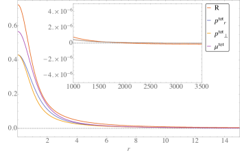
Figure 1: Solutions to the Starobinsky model with $\alpha=0.001$. The parameter values are: $\mu_{1}=-1.09$, $\mathcal{R}=5000$, $c_{1}=0.3$, and $A=2.3$.

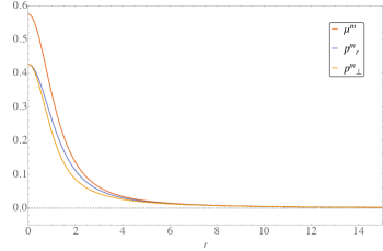
Figure 2: The matter fluid solutions. The energy density, radial and tangential pressure all satisfy the physical conditions in §VI. The parameter values are: $\mu_{1}=-1.09$, $\mathcal{R}=5000$, $c_{1}=0.3$, and $A=2.3$.

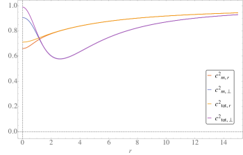
Figure 3: The radial and tangential speed of sound for the matter fluid, and the speed of sound for the total radial and perpendicular fluid quantities. The causal conditions as stated in §VI are obeyed. The parameter values are: $\mu_{1}=-1.09$, $\mathcal{R}=5000$, $c_{1}=0.3$, and $A=2.3$.

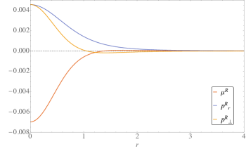
Figure 4: The curvature fluid solutions. The parameter values are: $\mu_{1}=-1.09$, $\mathcal{R}=5000$, $c_{1}=0.3$, and $A=2.3$.

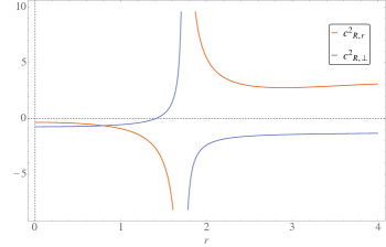
Figure 5: The speed of sound for the curvature fluid. The parameter values are: $\mu_{1}=-1.09$, $\mathcal{R}=5000$, $c_{1}=0.3$, and $A=2.3$.

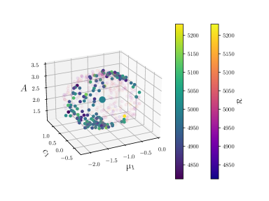
(a) The opaque points are the random values generated constrained to a sphere of radius 1 away from the central point. The darker points away from the center are the points that satisfy the causal condition $0<c_{m,r}^{2}\leq 1$.

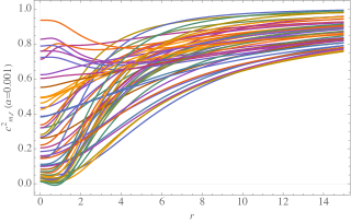
(b) Solutions to the radial speed of sound for the matter fluid using the set of parameter values that satisfy the causal condition as in Fig. 6(a). For illustrative purposes, only 50 solutions are plotted.

Figure 6: Generation of 500 random sets of parameter values with a radial shift of $0.05$ and constrained to a sphere of radius 1, using the parameter values in Fig. 1 as the central point of the sphere. Out of the 500 random sets of parameter values, only 154 satisfy the causal condition.

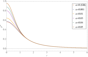
(a) Energy density of the matter fluid for varied values of $\alpha$.

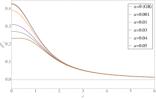
(b) Radial pressure of the matter fluid for varied values of $\alpha$.

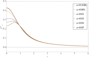
(c) Tangential pressure of the matter fluid for varied values of $\alpha$.

Figure 7: Matter fluid solutions for varied values of $\alpha$ using the same parameter values as in Fig. 1.

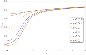
(a) Radial speed of sound of the matter fluid for varied values of $\alpha$.

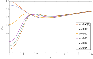
(b) Tangential speed of sound of the matter fluid for varied values of $\alpha$.

Figure 8: The radial and tangential speed of sound of the matter fluid for varied values of $\alpha$ using the same parameter values as in Fig. 1.

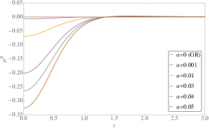
(a) Energy density of the curvature fluid for varied values of $\alpha$.

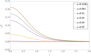
(b) Radial pressure of the curvature fluid for varied values of $\alpha$.

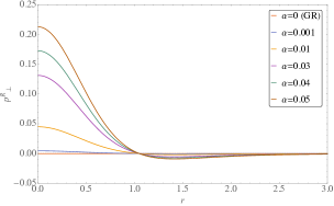
(c) Tangential pressure of the curvature fluid for varied values of $\alpha$.

Figure 9: Curvature fluid solutions for varied values of $\alpha$ using the same parameter values as in Fig. 1.

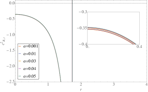
(a) Radial speed of sound of the curvature fluid for varied values of $\alpha$.

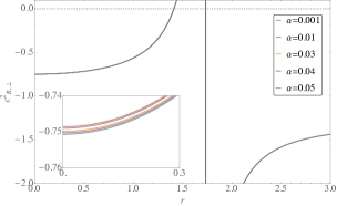
(b) Tangential speed of sound of the curvature fluid for varied values of $\alpha$.

Figure 10: The radial and tangential speed of sound of the curvature fluid for varied values of $\alpha$ using the same parameter values as in Fig. 1. The divergent behaviour we see is due to the corresponding energy density having a maximum around the value of $r$ where this divergence occurs, for all values of $\alpha$.

VIII Discussion and Conclusion

We presented a study that shows the extension of the TOV equations to the case of theories of gravity of order four, which are characterized by a non-linear action in the Ricci scalar: the so-called $f(R)$ theories of gravity.

By employing the (1+1+2) formalism, we have rewritten the TOV equations in a covariant and dimensionless form, valid for any function $f$. This result was achieved by recognizing that $f(R)$-gravity can always be recast as GR plus two effective, non-interacting fluids, one of which is not a perfect fluid.

The generalized TOV equations can then be used as a framework for finding exact, analytical solutions to static spherically symmetric spacetimes, which can describe compact stellar objects for $f(R)$-gravity. In this context, the work developed in NCD ; NCD2 can be applied to searching for new exact solutions of the TOV equations. In particular, we have made use of the so-called reconstruction algorithm of NCD ; NCD2 , in which a solution to the matter fluid can be found by making an ansatz of the description of the metric tensor. As noted in the previous section, not all solutions found this way are physical since the fluid sources have to satisfy specific physical requirements such as energy conditions, causality, etc.

Another important issue in the construction of meaningful interior solutions is the solution’s boundary connection with an exterior spacetime. It is well known that $f(R)$-gravity requires additional constraints to be joined smoothly to a vacuum spacetime connected with an additional (scalar) degree of freedom carried by the curvature scalar. This requirement makes the search for exact solutions much harder than in the context of GR.

As an example of the general procedure, we have considered the Starobinsky model in which the gravitational action is represented by a quadratic polynomial where the cosmological constant is excluded. Next, as ansatz on the metric tensor, we choose $k_{1}$ to be described by the corresponding interior Schwarzschild metric coefficient, and $k_{2}$ to be described by the corresponding Tolman IV metric coefficient. This choice was motivated by the attempt to preserve the physically relevant features of these metrics in terms of the Newtonian limit and simplicity. In addition, as shown in NCD ; NCD2 , this hybrid-styled metric describes an anisotropic fluid, thereby offering an ideal framework for $f(R)$-gravity.

On these premises, a solution obeying the physical and boundary constraints was found using the reconstruction algorithm. The solution we have found has interesting characteristics that can be highlighted by choosing some suitable value for the parameters. For example, in the case of a coupling constant $\alpha<<1$ with respect to the gravitational action ($\alpha=0.001$), this solution represents a fairly stiff matter distribution, meaning that the speed of sound is always above 0.5 in natural units. As the object is intrinsically anisotropic, the radial and orthogonal speeds of sound differs in behavior. The tangential speed of sound, in particular, has a minimum at a certain radial distance from the center, which corresponds to a maximum of the anisotropy. Indeed, comparing the behavior of the tangential and radial pressures, we see that with these parameters, this solution represents a “quasi-isotropic object” (similar to the ones found in sante-TOV-aniso-GR1 for the single fluid case) in the sense that the radial and tangential pressures behave similarly. Note that the effective fluid generated by the curvature invariants appears to have an energy density and pressure considerably smaller than the ones of baryonic matter. Therefore, the new solution represents an object mostly made of baryonic matter. The curvature fluid also presents a positive energy density and pressure but has a non-trivial speed of sound. More specifically, the speed of sound of the effective fluid can be negative and has a divergence due to the existence of a maximum for the energy density of the effective fluid and is therefore not pathological. As the value of $\alpha$ increases, we see that the pressure of the curvature fluid increases together with the energy density of baryonic matter, but the pressures of the matter fluid generally decrease. Interestingly, the speeds of sound of matter change dramatically close to the center, becoming quickly negative, whereas there seems to be hardly any change in the speeds of sound of the curvature fluid. It is then clear that the structure and the response to the parameter variation of compact stellar objects in $f(R)$-gravity can be very different with respect to the GR case. In turn, this result points to the fact that in modifying General Relativity, important physical structures, and composition differences might arise, which might one day become measurable.

All in all, our work shows that it is possible to use analytical approaches to describing astrophysical phenomena in $f(R)$-gravity and that these solutions can possess the correct physical features. Future work will be dedicated to improving the understanding of the properties of these solutions with particular emphasis on the observable features that might constitute a signature to test higher-order corrections with compact stellar objects.

Appendix A Solutions to the Starobinsky gravity case

A.0.1 Ricci scalar:

$$R(r)=-\frac{2\left(A^{4}\left(3c_{1}^{2}\mathit{z}{}^{3}+c_{1}a_{1}+\mathit{z}a_{2}\right)+A^{2}\left(c_{1}^{2}\mathit{z}{}^{3}\left(7r^{2}+3\mathcal{R}^{2}\right)+c_{1}a_{3}+\mathit{z}a_{4}\right)+2r^{2}\left(c_{1}^{2}\mathit{z}{}^{3}\left(3r^{2}+\mathcal{R}^{2}\right)+3c_{1}a_{5}+\mathit{z}a_{6}\right)\right)}{\mathcal{R}^{2}\left(A^{2}+2r^{2}\right)^{2}\mathit{z}\left(c_{1}\mathit{z}-\mu_{1}r^{2}+3\right){}^{2}},$$ (98)

where $\mathit{z}=\sqrt{3-\mu_{1}r^{2}}$, and

$$a_{1}=\left(9\mu_{1}^{2}r^{4}-2\mu_{1}r^{2}\left(\mu_{1}\mathcal{R}^{2}+24\right)+9\left(\mu_{1}\mathcal{R}^{2}+6\right)\right),$$ (99)

$$a_{2}=\left(6\mu_{1}^{2}r^{4}-2\mu_{1}r^{2}\left(\mu_{1}\mathcal{R}^{2}+15\right)+9\left(\mu_{1}\mathcal{R}^{2}+3\right)\right),$$ (100)

$$a_{3}=\left(22\mu_{1}^{2}r^{6}+\mu_{1}r^{4}\left(\mu_{1}\mathcal{R}^{2}-117\right)-6r^{2}\left(2\mu_{1}\mathcal{R}^{2}-21\right)+54\mathcal{R}^{2}\right),$$ (101)

$$a_{4}=\left(15\mu_{1}^{2}r^{6}-\mu_{1}r^{4}\left(2\mu_{1}\mathcal{R}^{2}+75\right)+r^{2}\left(6\mu_{1}\mathcal{R}^{2}+63\right)+27\mathcal{R}^{2}\right),$$ (102)

$$a_{5}=\left(3\mu_{1}^{2}r^{6}-16\mu_{1}r^{4}+r^{2}\left(18-\mu_{1}\mathcal{R}^{2}\right)+6\mathcal{R}^{2}\right),$$ (103)

$$a_{6}=\left(6\mu_{1}^{2}r^{6}-\mu_{1}r^{4}\left(\mu_{1}\mathcal{R}^{2}+30\right)+3r^{2}\left(\mu_{1}\mathcal{R}^{2}+9\right)+9\mathcal{R}^{2}\right).$$ (104)

A.0.2 Total energy density:

$$\mu^{\text{tot}}=\frac{3A^{4}+A^{2}\left(7r^{2}+3\mathcal{R}^{2}\right)+2r^{2}\left(3r^{2}+\mathcal{R}^{2}\right)}{\mathcal{R}^{2}\left(A^{2}+2r^{2}\right)^{2}}.$$ (105)

A.0.3 Total isotropic pressure:

$$p^{\text{tot}}=\frac{-\left(A^{4}\left(3c_{1}^{2}\mathit{z}{}^{3}+2c_{1}b_{1}+\mathit{z}b_{2}\right)\right)-A^{2}\left(c_{1}^{2}\mathit{z}{}^{3}\left(7r^{2}+3\mathcal{R}^{2}\right)+2c_{1}b_{3}+\mathit{z}b_{4}\right)-2r^{2}\left(c_{1}^{2}\mathit{z}{}^{3}\left(3r^{2}+\mathcal{R}^{2}\right)+2c_{1}b-{5}+3\mathit{z}b_{6}\right)}{3\mathcal{R}^{2}\left(A^{2}+2r^{2}\right)^{2}\mathit{z}\left(c_{1}\mathit{z}-\mu_{1}r^{2}+3\right){}^{2}},$$ (106)

where

$$b_{1}=\left(\mu_{1}\left(6\mu_{1}r^{4}-2r^{2}\left(\mu_{1}\mathcal{R}^{2}+15\right)+9\mathcal{R}^{2}\right)+27\right),$$ (107)

$$b_{2}=\left(\mu_{1}r^{2}\left(9\mu_{1}r^{2}-4\mu_{1}\mathcal{R}^{2}-42\right)+18\mu_{1}\mathcal{R}^{2}+27\right),$$ (108)

$$b_{3}=\left(r^{2}\left(\mu_{1}r^{2}\left(15\mu_{1}r^{2}-2\mu_{1}\mathcal{R}^{2}-75\right)+6\mu_{1}\mathcal{R}^{2}+63\right)+27\mathcal{R}^{2}\right),$$ (109)

$$b_{4}=\left(r^{2}\left(\mu_{1}r^{2}\left(23\mu_{1}r^{2}-7\mu_{1}\mathcal{R}^{2}-108\right)+30\mu_{1}\mathcal{R}^{2}+63\right)+27\mathcal{R}^{2}\right),$$ (110)

$$b_{5}=\left(r^{2}\left(\mu_{1}r^{2}\left(6\mu_{1}r^{2}-\mu_{1}\mathcal{R}^{2}-30\right)+3\mu_{1}\mathcal{R}^{2}+27\right)+9\mathcal{R}^{2}\right),$$ (111)

$$b_{6}=\left(r^{2}\left(\mu_{1}r^{2}\left(3\mu_{1}r^{2}-\mu_{1}\mathcal{R}^{2}-14\right)+4\mu_{1}\mathcal{R}^{2}+9\right)+3\mathcal{R}^{2}\right).$$ (112)

A.0.4 Total radial pressure:

$$p_{r}^{\text{tot}}=\frac{4\left(A^{2}+r^{2}\right)\left(\mathcal{R}^{2}-r^{2}\right)}{r^{2}\mathcal{R}^{2}\left(A^{2}+2r^{2}\right)}\left(-\frac{\mathcal{R}^{2}\left(A^{2}+2r^{2}\right)}{4\left(A^{2}+r^{2}\right)\left(\mathcal{R}^{2}-r^{2}\right)}+\frac{\mu_{1}r^{2}}{-2c_{1}\mathit{z}+2\mu_{1}r^{2}-6}+\frac{1}{4}\right).$$ (113)

A.0.5 Total perpendicular pressure:

$$p_{\perp}^{\text{tot}}=\frac{A^{4}\left(-c_{1}^{2}\mathit{z}{}^{3}+c_{1}d_{1}+\mathit{z}d_{2}\right)-A^{2}\left(c_{1}^{2}\mathit{z}{}^{3}\left(2r^{2}+\mathcal{R}^{2}\right)+3c_{1}d_{3}+\mathit{z}d_{4}\right)-2r^{4}\left(c_{1}^{2}\mathit{z}{}^{3}-c_{1}d_{1}+\mathit{z}d_{5}\right)}{\mathcal{R}^{2}\left(A^{2}+2r^{2}\right)^{2}\mathit{z}\left(c_{1}\mathit{z}-\mu_{1}r^{2}+3\right){}^{2}},$$ (114)

where

$$d_{1}=\left(\mu_{1}r^{2}\left(-4\mu_{1}r^{2}+\mu_{1}\mathcal{R}^{2}+21\right)-6\mu_{1}\mathcal{R}^{2}-18\right),$$ (115)

$$d_{2}=\left(\mu_{1}r^{2}\left(-3\mu_{1}r^{2}+\mu_{1}\mathcal{R}^{2}+15\right)-6\mu_{1}\mathcal{R}^{2}-9\right),$$ (116)

$$d_{3}=\left(r^{2}\left(\mu_{1}\left(3\mu_{1}r^{4}-16r^{2}+\mathcal{R}^{2}\right)+12\right)+6\mathcal{R}^{2}\right),$$ (117)

$$d_{4}=\left(r^{2}\left(\mu_{1}r^{2}\left(7\mu_{1}r^{2}-\mu_{1}\mathcal{R}^{2}-36\right)+9\mu_{1}\mathcal{R}^{2}+18\right)+9\mathcal{R}^{2}\right),$$ (118)

$$d_{5}=\left(\mu_{1}r^{2}\left(3\mu_{1}r^{2}-\mu_{1}\mathcal{R}^{2}-15\right)+6\mu_{1}\mathcal{R}^{2}+9\right).$$ (119)

References

- (1) H. A. Buchdahl, MNRAS 150, 1 (1970); A. A. Starobinsky, Phys. Lett. B 91, 99 (1980).
- (2) S. Carloni, P. K. S. Dunsby and A. Troisi, Phys. Rev. D 77, 024024 (2008) [arXiv:0707.0106 [gr-qc]]; K. N. Ananda, S. Carloni and P. K. S. Dunsby, Phys. Rev. D 77, 024033 (2008) [arXiv:0708.2258 [gr-qc]]; S. Carloni, K. N. Ananda, P. K. S. Dunsby and M. E. S. Abdelwahab, arXiv:0812.2211 [astro-ph]; K. N. Ananda, S. Carloni and P. K. S. Dunsby, arXiv:0809.3673 [astro-ph]; K. N. Ananda, S. Carloni and P. K. S. Dunsby, arXiv:0812.2028 [astro-ph].
- (3) J. R. Oppenheimer, and G. M. Volkoff, Phys. Rev. 55, 4 (1939).
- (4) M. S. R. Delgaty, and K. Lake, Computer Physics Communications, 115, 2-3 (1998).
- (5) G. J. Olmo, D. Rubiera-Garcia and A. Wojnar, Phys. Rept. 876, 1 (2020).
- (6) C. A. Clarkson and R. K. Barrett, Class. Quant. Grav. 20, 3855 (2003); C. Clarkson, Phys. Rev. D 76, 104034 (2007); G. Betschart and C. A. Clarkson, Class. Quantum Grav. 21 5587 (2005).
- (7) C. A. Clarkson, M. Marklund, G. Betschart and P. K. S. Dunsby, 2003 Astrophys.J. 613 492-505 (2004).
- (8) A. M. Nzioki, S. Carloni, R. Goswami and P. K. S. Dunsby, Phys. Rev. D 81, 084028 (2010).
- (9) S. Carloni, P. K. S. Dunsby, General Relativity and Gravitation 48, 136 (2016).
- (10) S. Carloni and D. Vernieri, Phys. Rev. D D 97, 124056 (2018).
- (11) S. Carloni and D. Vernieri, Phys. Rev. D D 97, 124057 (2018).
- (12) P. Luz and S. Carloni, Phys. Rev. D 100 (2019) no.8, 084037 doi:10.1103/PhysRevD.100.084037 [arXiv:1907.11489 [gr-qc]].
- (13) N. F. Naidu, S. Carloni, P. K. S. Dunsby, Phys. Rev. D 104, 044014 (2021).
- (14) N. F. Naidu, S. Carloni, P. K. S. Dunsby, Phys. Rev. D 106, 124023 (2022).
- (15) B. S. DeWitt, Gordon & Breach, New York, 1965.
- (16) N. H. Barth and S. M. Christensen, Phys. Rev. D 28, 1876 (1983).
- (17) J. Ehlers Abh. Mainz Akad. Wiss. u. Litt. (Math. Nat. kl) 11 (1961); G. F. R. Ellis, in General Relativity and Cosmology, Proceedings of XLVII Enrico Fermi Summer School, ed . R. K, Sachs (New York Academic Press, 1971); G. F. R. Ellis and H. van Elst, Cosmological models (Cargèse lectures 1998), in Theoretical and Observational Cosmology, edited by M. Lachièze-Rey, p. 1 (Kluwer, Dordrecht, 1999).
- (18) J. M. Bardeen, Phys. Rev. D 22, 1882 (1980); G. F. R. Ellis & M. Bruni Phys. Rev. D 40 1804 (1989); M. Bruni, P. K. S. Dunsby & G. F. R. Ellis, Ap. J. 395 34 (1992); G. F. R. Ellis, M. Bruni and J. Hwang, Phys. Rev. D 42 (1990) 1035 (1990); P. K. S. Dunsby, M. Bruni and G. F. R. Ellis, Astrophys. J. 395, 54 (1992); M. Bruni, G. F. R. Ellis and P. K. S. Dunsby, Class. Quant. Grav. 9, 921 (1992); P. K. S. Dunsby, B. A. C. Bassett and G. F. R. Ellis, Class. Quant. Grav. 14, 1215 (1997); [arXiv:gr-qc/9811092]; P. K. S. Dunsby and M. Bruni, Int. J. Mod. Phys. D 3, 443 (1994) [arXiv:gr-qc/9405008].
- (19) P. K. S. Dunsby, Class. Quant. Grav. 14, 3391 (1997) [arXiv:gr-qc/9707022]; A. Challinor and A. Lasenby, Phys. Rev. D 58 023001; Astrophys. J. 513 1 (1999); R. Maartens, T. Gebbie and G. F. R. Ellis, Phys. Rev. D 59 083506 (1999).
- (20) W. Israel, Nuovo Cimento, 44, 1 (1966).
- (21) N. Deruelle, M. Sasaki and Y. Sendouda, Prog. Theor. Phys. 119, 237-251 (2008).
- (22) J. M. M. Senovilla, Phys. Rev. D, vol. 88, p. 064015, (2013).
- (23) J. M. M. Senovilla, Class. Quantum Grav. 31, 072002 (2014).
- (24) A. Ganguly, R. Gannouji, R. Goswami and R. Subharthi, Phys. Rev. D 89 064019 (2014); S. S. Yazadjiev, D. D. Doneva, K. D. Kokkotas and K. V. Staykov, J CAP 06, 003 (2014); M. Aparicio Resco, A. de la Cruz-Dombriz, F. Llanes Estrada, V. Zapatero Castrillo, Phys. Dark Univ. 13, 147 (2016); A. V. Astashenok, S. D. Odintsov, A. de la Cruz-Dombriz, Class. Quantum Grav. 34, 205008 (2017); P. Feola, X. J. Forteza, S. Capozziello, R. Cianci, S. Vignolo, Phys. Rev. D 101, 044037 (2020).
- (25) S. Mignemi and D. L. Wiltshire, Phys. Rev. D 46, 1475 (1992).
- (26) J. Naf and P. Jetzer, Phys. Rev. D 81, 104003 (2010).