Imprints of interaction processes in the globular cluster system of NGC 3640

Abstract

We present a wide-field study of the globular cluster systems (GCS) of the elliptical galaxy NGC 3640 and its companion NGC 3641, based on observations from Gemini Multi-Object Spectrograph/Gemini. NGC 3640 is a shell galaxy which presents a complex morphology, which previous studies have indicated as the sign of a recent ‘dry’ merger, although whether its nearest neighbour could have had an influence in these substructures remains an open question. In this work, we trace the spatial distribution of the globular clusters (GCs) as well as their colour distribution, finding a potential bridge of red GCs that connects NGC 3640 to its less massive companion, and signs that the blue GCs were spatially disturbed by the event that created the shells.

1 Introduction

Mergers are essential parts of the current $\Lambda$ Cold Dark Matter paradigm, in which dark matter haloes and galaxies are mainly formed through hierarchical assembly (Peebles, 1982; Blumenthal et al., 1984; Davis et al., 1985). In particular, the early evolution of early-type galaxies (ETGs) is dominated by major mergers involving large amounts of gas (Naab et al., 2007). Once they become quiescent, they continue to grow their mass and size through minor dry mergers, with little to no star formation (Naab et al., 2009, e.g.). Aside from being the driving forces behind the mass growth of a galaxy, mergers shape the morphology of galaxies (Hopkins et al., 2010; Kannan et al., 2015, e.g), feed central supermassive black holes, and potentially trigger central starbursts (Ellison et al., 2011; Satyapal et al., 2014). As such, they are important components of any galaxy formation model.

The frequency of major mergers experienced by a galaxy is influenced by the local density where it resides, as evidenced by the dependence of the fraction of passive galaxies and stellar mass functions with it (e.g. McNaught-Roberts et al., 2014; Etherington et al., 2017). Although this relation is nuanced, it is clear that higher-density environments show larger rates of galaxy mergers, with groups being the most active type of environment.

Tidal features are the most direct evidence of recent mergers, and they have been widely used to characterize the impact of these events on the properties of galaxies. Photometric analysis has shown, for example, that blue ETGs are more likely to present morphological disturbances (Tal et al., 2009; Kaviraj et al., 2011, e.g), hinting at the presence of younger stellar populations as a consequence of recent mergers. However, most of the signatures of accretion events are found in the form of low surface brightness structures, which require long exposures to be analysed.

Globular clusters (GCs) located in the halo of galaxies are helpful tools when it comes to tracing the occurrence of recent mergers since they are bright and they are connected to the underlying stellar population, acting as fossil records of the evolutionary history of their host galaxy and carrying in their properties valuable information about its accretion events. In regions where the stellar halo is too faint, GCs have been used as tracers of stellar streams and tidal tails (Napolitano et al., 2022), and when structures can be detected, the colours and positions of the GCs connected to them can shed further light on their origin (Lim et al., 2017; D’Abrusco et al., 2022, e.g). Since GCs are sparse even in massive galaxies and tidal features are hard to detect, studying this connection requires deep, wide-field observations. In nearby ETGs, rich underlying substructure is related with GC systems with unusual colour and luminosity distributions (e.g. Sesto et al., 2016; Bassino & Caso, 2017), and the presence of young GCs (e.g. Strader et al., 2004; Woodley et al., 2010).

The elliptical galaxy NGC 3640, located at a distance of 27 Mpc according to the results from the surface brightness fluctuation method (SBF) (Tully et al., 2013), is part of a loose group conformed by approximately eight galaxies (Madore et al., 2004). This group is thought to be dynamically young since no X-ray emission was detected by ROSAT above $3\,\sigma$ of the background level (Osmond & Ponman, 2004). NGC 3640 has an absolute magnitude of $\textrm{M}_{\textrm{B}}=-20.93$ (Tal et al., 2009), and it has been classified as both E3 (de Vaucouleurs et al., 1991) and T3 (Kormendy, 1982), the latter being defined as a type for galaxies with very prominent companions, making the probability of tidal effects very high. Its close companion, NGC 3641 is classified as a compact elliptical (cE) in de Vaucouleurs et al. (1976), and it is located at a projected angular distance of $2^{\prime}5$ South. If we consider the distance to NGC 3640 as the mean distance to the group, this corresponds to a physical distance of $19\,\textrm{kpc}$.

Prugniel et al. (1988) (P88 for the rest of this work) present the first analysis dedicated to the morphology of this galaxy and its kinematics. Using photometry, they analyse the surface brightness profile of NGC 3640, identifying signatures of a recent merger in the shape of the isophotes and in the residual structures. A previous work had already shown the isophotes to be boxy (Bender et al., 1988), and more recently, NGC 3640 has even been referred to as an example of ‘extreme boxyness’ (Michard & Prugniel, 2004). In P88, they also detect a dust lane along the minor axis, a feature that has been identified in remnants of merger processes with large quantities of gas and dust. With additional long-slit spectroscopic data, P88 characterize NGC 3640 as a fast rotator ($V/\sigma=1.5)$, which can also be a consequence of an interaction or merging process. In comparison with other galaxies thought to be merger remnants, they argue NGC 3640 appears to be at a more advanced stage of relaxation, though it lacks strong nuclear radio emission, which is expected to be ignited after the merging has been completed. Since NGC 3640 shows very small amounts of gas and dust according to P88, the merger it experienced is thought to have been ‘dry’.

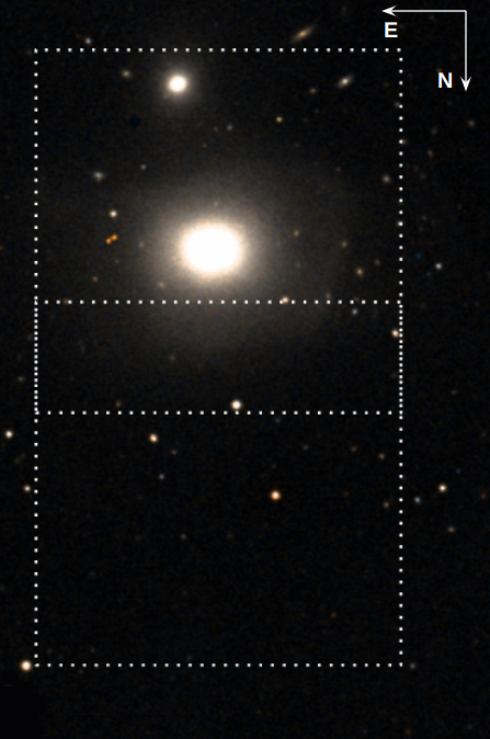
Figure 1: Representation of the observed GMOS fields plotted over a colored image from the Digitized Sky Survey 2, obtained from the Aladin Sky Atlas.

Later on, Schweizer & Seitzer (1992) include NGC 3640 in a sample of galaxies they analyze using an index defined in their work to quantify features connected to mergers. Out of the 35 ellipticals in the sample, NGC 3640 presents one of the highest values of this index, meaning it is among the most disturbed galaxies. Assuming this disturbance is owed to NGC 3640 being the result of a disk-disk merger, they use its UBV colour to date this merger, concluding it could be a ‘young’ elliptical, i.e. less than 7 Gyr old. However, they point out in their work that the presence of NGC 3641 could have had a significant influence in the disturbances detected in NGC 3640, especially considering the high interactivity between galaxies in small groups. Michard & Prugniel (2004) support the idea of NGC 3640 having been formed in a major merger based on its morphology and on their analysis of its stellar population indicators, which indicate the presence of a relatively small young population, in comparison with other highly disturbed galaxies. In addition, two different works performed analysis of the stellar population of NGC 3640 using long-slit spectra. While Denicoló et al. (2005) estimate a nuclear age of 2.5 Gyr, the reanalysis of the same data by Brough et al. (2007) finds an older (4 Gyr), less metal-rich center, which they estimate to be within $1.5\sigma$ of their results. Overall, their analysis points to NGC 3640 having undergone a dissipational merger 7.5 Gyr ago, and presenting a younger central age that would imply a more recent ‘wet’ merger.

NGC 3640 shows then a large number of peculiarities, including a collection of signs that point at it having undergone a relatively recent merging process. Though several of these signs have been associated with a major disk-disk merger, none of the analyses rule out interactions with the less massive galaxies in the group as the cause of some of the tidal disturbances. The compactness of NGC 3641 could be another hint of interaction since it could be a consequence of tidal stripping. This is inconclusive since NGC 3641 is located to the South of NGC 3640, while the major axis of NGC 3640 is oriented East to West, and its classification as a cE is unclear. There are many open questions about the evolutionary history of NGC 3640, particularly in terms of its interaction with NGC 3641. In this work, we study the globular cluster system (GCS) of both galaxies, looking for clues that can help us untangle the interactions that have shaped NGC 3640.

In Section 2, we describe the data and the reduction process. In Sections 3 and 4 we analyse several properties of the GCS of NGC 3640 and NGC 3641, respectively. In Section 5 we focus on the connection between the spatial distribution of GCs and the low surface brightness structures. In Section 6 we discuss the results. Finally, in Section 7 we summarize our results.

2 Data acquisition and reduction

2.1 Observations

Filter	$\lambda$ [nm]	Exposition time [s]
$g^{\prime}$	475	4 x 650
$r^{\prime}$	630	4 x 270
$i^{\prime}$	780	4 x 240

Table 1: Exposition times for each filter, identical for both fields.

The observations for this work were taken utilizing the Gemini Multi-Object Spectrograph Camera (GMOS) on Gemini North (Program GN-2016A-Q-69, PI: L. Bassino) on February 10th, 2016, in imaging mode. The field of view of GMOS is of $5.5\,\rm{arcmin}\times 5.5\,\rm{arcmin}$, and we used a binning of $2\times 2$, which results in a resolution of $0.146\,\rm{arcsecpix}^{-1}$. The seeing for these observations was $\approx 0.75$ across all filters. We observed two fields as shown in Figure 1, one containing both galaxies and an adjacent one with which we aimed to cover the entire extension of the GCS and calculate the background contamination. We also observed the Landolt field of standard stars SA 104 (Landolt, 1992), using the magnitudes obtained in the GMOS filters by Jørgensen (2009).

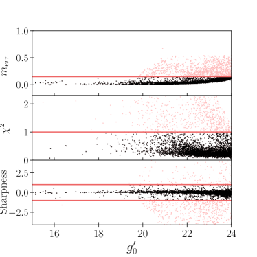
Figure 2: From top to bottom, the error in magnitude, $\chi^{2}$ and the sharpness value obtained from PSF photometry for the $g^{\prime}$ filter for reference. Solid lines indicate the chosen limits, with the limit in magnitude applied to the selections in the following tests.

2.2 Data reduction and point-source selection

We used the DRAGONS Data Reduction Software (Labrie et al., 2019) to correct the observations using bias and flat-field images obtained from the Gemini Archive , and then to combine all of the images corresponding to each field in each filter. Images in the filter $i^{\prime}$ presented a fringe pattern which was corrected using a blank field from the Archive. We then proceeded to subtract a model of the integrated light from both galaxies using the median filter task in SciPy. We ran it twice with different-sized windows (100 and 50 pixels), allowing for the detection of point-like sources in the inner region. Finally, we used geomap and geotran in IRAF to geometrically transform the final images, taking them all to the same reference system and cropping the edges.

The first catalog of globular cluster candidates present in the field was built using Source Extractor (Bertin & Arnouts, 1996). We used two filters, Gaussian and Mexhat ones, since the latter has proven to be more effective in crowded regions. Combining the outcome of both, we obtained approximately 4000 objects. Considering GCs appear as unresolved point-like sources at this distance, we use the classifier $CLASS\_STAR$, which estimates the probability of the detected source being point-like. In this case, we eliminate from the sample objects with $CLASS\_STAR>0.5$ as to clear it of extended objects, mainly background galaxies and saturated stars.

We obtained aperture photometry for these objects using the tasks in the DAOPHOT package in IRAF. After selecting $\sim 30$ of the brightest objects in each filter, for each field correspondingly, we built the spatially variable corresponding point-spread function (PSF) and obtained PSF photometry of our sample with the task ALLSTAR.

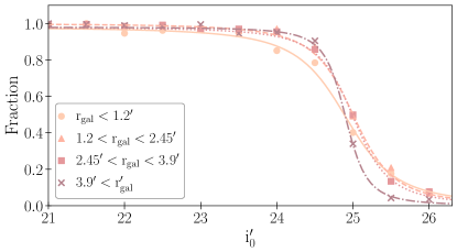
Figure 3: Completeness fraction in the $i^{\prime}$ filter for three concentric annular regions, with the corresponding fit. Circles and a solid line indicate the inner region; triangles and a dashed line, the intermediate region; and squares and a dotted line, the outer region.

Besides calculating instrumental magnitudes with their errors, this task provides us with statistical parameters that characterize the goodness of the fit. In particular, it calculates the sharpness and the chi-squared. In the completeness test described in the following section, we obtained the distribution of parameters for a large number of artificial sources, and selected constraints for these parameters, as shown in Figure 2. After applying this selection, we obtain a total of $1576$ point-like sources.

2.3 Completeness test

In the dim end of the magnitudes range, we estimate the limiting value by performing a completeness test. We build a catalog of 32000 objects, with magnitudes assigned so that they cover the range of magnitudes and colours expected for old GCs, and positions that cover both fields, distributed evenly over 200 copies of the original image. Using the PSF obtained before, we add them as fake stars to our raw data. Then, we proceed to perform the same data reduction process as before, detecting point-like sources and performing PSF photometry in the same manner as for our GC candidates. This allows us to obtain the set of statistical parameters that return the highest fraction of sources while still providing a good fit.

We divide the area into three concentric annular regions to take into consideration any radial variations in the completeness, and we estimate the fraction of recovered sources per magnitude bin for each of these regions. Then, we fit a function to the completeness fraction estimated for each region, which will be used later on to apply a more detailed completeness correction (Figure 3). This is particularly relevant in the inner region, in which the intrinsic brightness of the galaxy causes the completeness fraction to be lower than in other areas of the image. Finally, we determine the overall limit as the magnitude at which this fraction is of $\sim 80\%$ for the intermediate and outer regions, which in this case is $i^{\prime}_{0}=24.7$.

2.4 Photometric calibration

We transform the instrumental magnitudes to the standard system by using the equations corresponding to the E2V-DD detector obtained from the Gemini Observatory website, described in Equation 1, and a field of standard stars, SA 104. We calculated the zero points and colour terms by fitting a curve to the relation between our photometry of the standard stars and their standard magnitudes (see Table 2). In the case of the median atmospheric extinction coefficients, $k_{CP}$, we used the ones provided by the Gemini Observatory website, corresponding to the median value at Mauna Kea.

$$\begin{split}m_{\rm std}=&m_{\rm zero}-2.5\,\log_{10}\left(N(e-)/\textrm{exptime}\right)\\ &-k_{CP}(\textrm{airmass}-1.0)\end{split}$$ (1)

Filter	Zero-point	Colour term
g’	$28.08\pm 0.06$	$0.06\pm 0.09*(g^{\prime}-r^{\prime})$
r’	$28.23\pm 0.11$	$0.01\pm 0.18*(g^{\prime}-r^{\prime})$
i’	$28.35\pm 0.03$	$0.13*(r^{\prime}-i^{\prime})$

Table 2: Zero-point and colour term values obtained for each filter. The colour term used for the $i^{\prime}$ filter was obtained from the Gemini website since the quality of the observations of the standard stars field in said filter did not allow for a good fit.

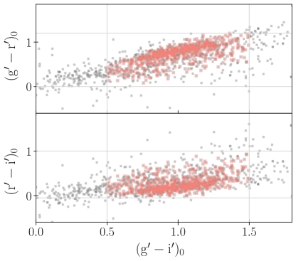
Figure 4: Colour-colour diagrams for two different combinations of filters, showing all sources present in the field as grey crosses, and those that satisfy all the criteria to be considered GC candidates are highlighted with pink squares. The limits shown in solid lines are estimated based on values from the literature.

2.5 GC candidate selection

In Figure 4, we show the colour-colour diagrams of the entire sample of point-like sources detected in the field. We use colour limits to identify GC candidates, following Bassino & Caso (2017), in the three classic colour combinations. The limits in $(g^{\prime}-i^{\prime})$ are shown in the colour-magnitude diagram (Figure 6), where we add the limit obtained from the completeness test, corresponding to $80\%$, in the dim end of the magnitudes axis. The colour limits correspond to $0.4<(g^{\prime}-i^{\prime})_{0}<1.5$, $0.3<(g^{\prime}-r^{\prime})_{0}<1.2$ and $-0.05<(r^{\prime}-i^{\prime})_{0}<0.5$. In addition, we limit the error in magnitude to $<0.15$, and we exclude objects brighter than $M_{i}=21.5$, which at the estimated distance for NGC 3640 corresponds to $M_{V}=-11$, which is the limit at which the probability of finding GCs becomes very low (Harris et al., 2014). Objects brighter than this limit that fall in this colour range are more likely to be ultra-compact dwarfs, and as such, we treat them as potential contaminants.

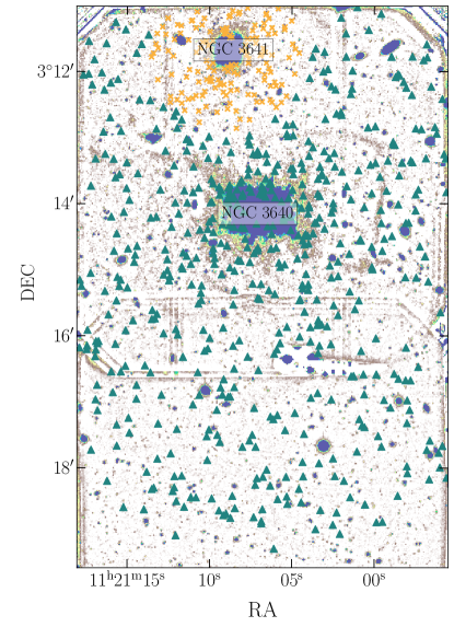
Figure 5: Spatial distribution of all GC candidates across both fields. Orange dots and green diamonds indicate sources attributed to NGC 3640 and NGC 3641 respectively. The centre of each galaxy is shown in large symbols with thick edges.

Since we cannot estimate radial velocity measurements from photometry alone, initially we separate GC candidates according to their spatial distribution, as shown in Figure 5. The relation between the stellar mass of the galaxy and the extension of the GCS shown in Equation 9 in Caso et al. (2019) results in a value of $21\,kpc$ for the extension of the GCS of NGC 3641. However, the fact that NGC 3641 is a compact elliptical means that the estimated extension of the GCS that corresponds to the effective radius of the galaxy is far smaller. Since existing scaling relations are inconclusive for cE galaxies, we initially attribute all GC candidates within a radius of $75^{\prime\prime}$ of the center of NGC 3641 to its GCS, and the rest to NGC 3640, though this separation is by no means conclusive.

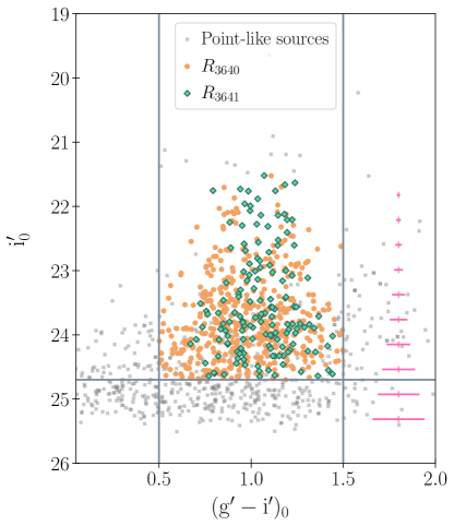
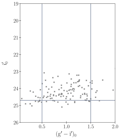
Figure 6: Left: Colour-magnitude diagram for all sources, shown as grey crosses. The GC candidates attributed by galactocentric distance to NGC 3641 are shown as green diamonds, while those attributed to NGC 3640 are represented by orange dots. In pink we show the error bars for the mean error in magnitude bins ($0.4$ mag). Right: Colour-magnitude diagram for background sources.

3 The GCS of NGC 3640

3.1 Colour-magnitude diagram

In Figure 6 we show the colour-magnitude diagram of the point-like sources in the field and the GCs associated with each galaxy. NGC 3641 presents intermediate colours in comparison with NGC 3640, covering a smaller range in general. In particular, NGC 3641 almost lacks blue GCs. It is reasonable to expect those to have been accreted first if these galaxies have interacted.

NGC 3640 covers a range typical of GCS in massive ETGs, and towards the brighter end, two subpopulations are evident.

The right panel shows the background sources, located in the region selected as background based on the radial distribution described in the following section. The contamination level is even across the entire colour range.

3.2 Radial distribution

In Figure 7 we show the radial distribution for the GC candidates across both fields attributed to NGC 3640. We estimate the background level considering the flattening of the distribution in the outer regions, at $r_{gal}=3.7^{\prime}$, obtaining a contamination correction of $8\,\textrm{GC}\,\textrm{arcmin}^{-2}$ which was applied throughout the analysis.

We fit a Hubble-Reynolds law to the background corrected profile, resulting in the following profile:

$$n(r)=1.88\left(1+\left(\frac{r}{1.16}\right)^{2}\right)^{-2.06}$$ (2)

Extrapolating this function to the value at which it reaches $20\%$ of the background level, we calculate a total extension of the system of $31\,{\rm kpc}$ ($\approx 4^{\prime}$).

Integrating the profile up to this point, we obtain the total population up to our completeness level, resulting in $\approx 310\,$GCs.

In addition, in Figure 8, we show the radial distribution for GC candidates split into red and blue subpopulations, following the separation described in the following Section. We fit Hubble-Reynolds laws to both profiles, obtaining core radii of $0.72$ for blue GCs and $1.8$ for red GCs. The red subpopulation appears heavily concentrated towards the centre of the galaxy, whereas the blue one extends to the outer region in a steeper manner. These behaviours are consistent with what is expected if we consider red GCs to be mostly formed in-situ, and blue GCs to come from accretion processes that increase their density in the outer halo.

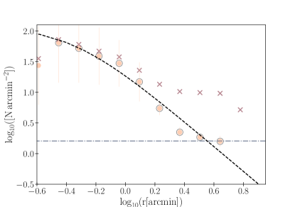
Figure 7: Radial distribution for GC candidates attributed to NGC 3640. Crosses describe the raw sample, while orange circles show the background corrected distribution, with a grey, larger circle indicating those considered for the fit. The dash-dotted line shows the level at which $20\%$ of the background density is reached, and the dashed curve, the Hubble-Reynolds law fit.

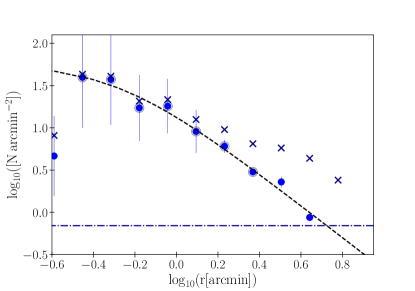
Figure 8: Radial distribution for GC candidates attributed to NGC 3640, for the blue (top) and red (bottom) subpopulations. Crosses describe the raw sample, while circles show the background corrected distribution. The dash-dotted horizontal line indicates $20\%$ of the background level, and the dashed curve, the Hubble Reynolds law.

3.3 Colour distribution

In Figure 9 we show the histogram of the colour distribution for the GCs attributed to NGC 3640, as well as the background correction. Since the background sources show a homogeneous distribution across the colour range, we consider the background correction negligible in terms of fitting the subpopulations.

Figure 10 shows the density probability functions of the colour distribution for the GCs attributed to NGC 3640, as well as the inner ($r_{gal}<75^{\prime\prime}$) and outer ($r_{gal}>75^{\prime\prime}$) regions. These smoothed distributions use a Gaussian kernel, with a bandwidth of $0.5$.

We use the Gaussian Mixture Modeling code (GMM, Muratov & Gnedin (2010)) to estimate the probability of the distribution being bimodal in all samples. The output provided by GMM includes both the parameters for the best fit of Gaussian functions ($\mu$ and $\sigma$, as well as the fraction of sources attributed to each mode) and statistical tests that estimate the confidence level of the multi-modal fit. These statistical tests are the kurtosis of the distribution, which quantifies its peakedness, and D, which is a parameter that is calculated by assuming bimodality and measuring the distance between the estimates means, weighed by the broadness of each mode. D is expected to be greater than 2 in bimodal distributions. A unimodal distribution would result in a stronger peak, which would in turn be reflected in positive values for the kurtosis.

In Table 3, we show the results for each sample. When considering the entire population of GCs attributed to NGC 3640, the result is a negative kurtosis and a $D>2$, meaning a bimodal distribution, with modal values similar to those in other massive early-type galaxies (Harris et al., 2009; Forbes et al., 2011).

Both regions are statistically bimodal according to this fit. The means of the subpopulations in the inner region are redder than when considering the entire sample, in particular for the red subpopulation. The outer region presents bluer means for both subpopulations than the entire sample, and is more likely to be contaminated by GCs connected to NGC 3641.

Sample	$\mu$		$\sigma$		Red fraction	Kurtosis	D
	Blue	Red	Blue	Red
NGC $3640$	$0.85\pm 0.04$	$1.19\pm 0.05$	$0.15\pm 0.02$	$0.14\pm 0.02$	$0.35$	$-0.56$	$2.27\pm 0.24$
NGC 3640 (inner)	$0.92\pm 0.05$	$1.24\pm 0.05$	$0.14\pm 0.03$	$0.12\pm 0.02$	$0.30$	$-0.56$	$2.54\pm 0.39$
NGC 3640 (outer)	$0.79\pm 0.05$	$1.13\pm 0.06$	$0.14\pm 0.02$	$0.16\pm 0.02$	$0.48$	$-0.60$	$2.22\pm 0.29$

Table 3: Parameters for the Gaussian functions resulting from the bimodal fit performed using GMM for the different samples.

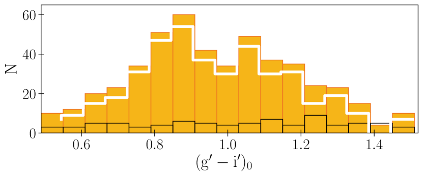
Figure 9: Colour distribution for the full sample of GC candidates attributed to NGC 3640 shown in orange. Black lines represent the background distribution, and white lines the corrected distribution.

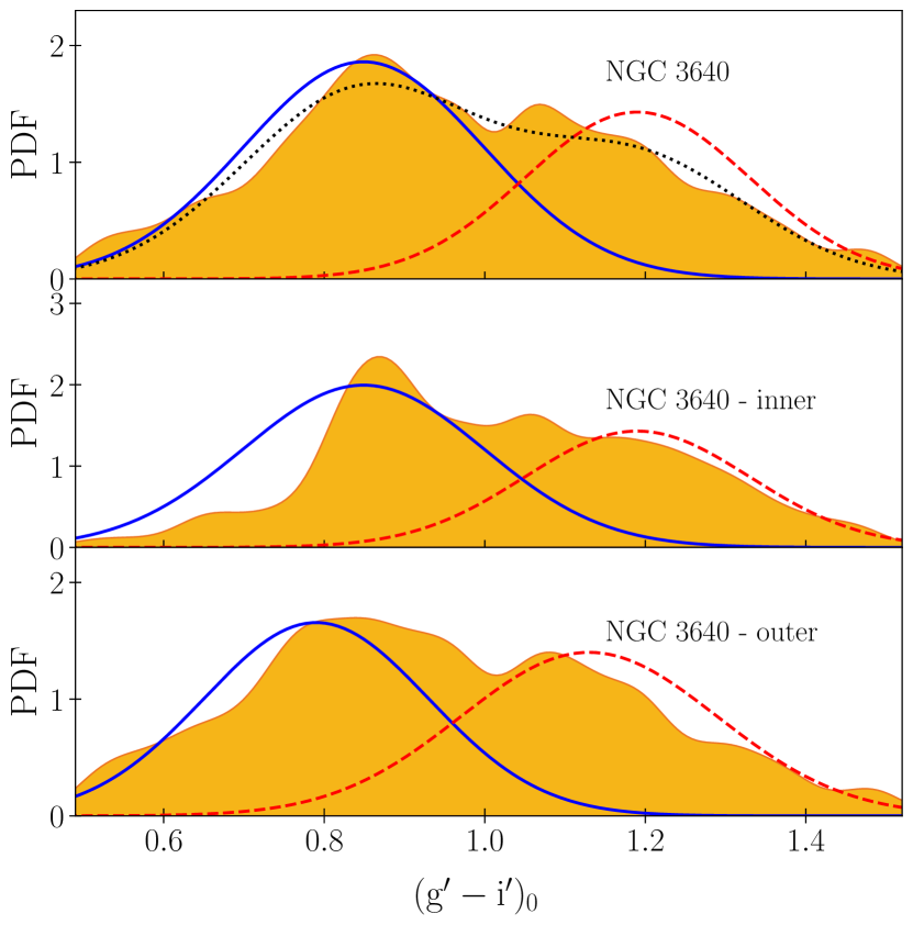
Figure 10: Smoothed olour distributions for the full sample of GC candidates attributed to NGC 3640 (top). In the middle panel, the inner region (left), and in the bottom, the outer region of NGC 3640. Blue solid curves and red dashed curves represent the best fit from GMM for bimodal Gaussian distributions for each sample.

3.4 Luminosity function

The luminosity function of globular cluster systems is widely used as a distance estimator due to the universality of the absolute magnitude of its turn-over. The SBF distance to NGC 3640 is $26.9$ Mpc, which results in a turn-over magnitude of $V_{0}=24.75$. Using the transformations from Faifer et al. (2011), and a mean $(g-i)$ value of 1, we can transform to approximately $i_{0}=24.1$, which is well within our completeness range, allowing us to estimate our own measurement of the distance to compare with the literature value.

In Figure 11, we show the luminosity function for GC candidates associated with NGC 3640, after applying a completeness and background correction. Fitting a Gaussian function to our distribution results in a turn-over value of $i_{0}=23.74\pm 0.02$, which is within error from the SBF distance. The dispersion of the Gaussian is $\sigma_{L}=0.68\pm 0.02$. In Harris et al. (2014), the GCLF is proposed to have an intrinsic width of $\sigma_{L}=0.52-0.55\,\textrm{dex}$. The difference between these two values may be due to contamination from NGC 3641.

Due to this slight difference, we choose to use the turn-over value from SBF to estimate the percentage of GCs within our completeness range in relation to the total population, which in this case is $74\%$. Combining this result with the number obtained from the integration of the radial distribution, we can estimate the total number of GCs for NGC 3640, $N_{GC}\approx 350$.

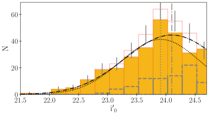
Figure 11: Luminosity function for the GC candidates associated with NGC 3640. Orange lines show the original distribution, with orange solid blocks showing the result after correcting for completeness and subtracting the background, indicated in dashed gray lines. The dashed curve and vertical line correspond to the fit performed in this work and its corresponding turn-over magnitude, while the dash-dotted is the fit obtained with the distance from the literature, with its fixed turn-over magnitude shown as a dash-dotted vetical line. All fits were done using only the shown magnitude range according to the completeness test, with the corrected distribution.

4 The GCS of NGC 3641

4.1 Radial distribution

In Figure 12 we show the radial distribution for the GCs within $75^{\prime\prime}$ of the centre of NGC 3641, with a Hubble-Reynolds law fit up to the imposed limit. If we extrapolate this profile to the same level we used for NGC 3640, we obtain an estimate for the population of NGC 3641 up to the completeness level of $\approx 100$ GCs.

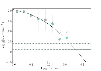
Figure 12: Radial distribution for GC candidates attributed to NGC 3641. Grey crosses describe the raw sample, while green dots show the background corrected distribution. A dashed curve shows the Hubble profile. A horizontal line indicates the same background level as in previous figures.

4.2 Colour distribution

In Figure 13 we show the colour distribution for GCs associated with NGC 3641. Analogously to the previous section, we use GMM and in this case obtain a negative kurtosis ($-0.384$) but the value of D is significantly smaller than 2 ($1.74$), indicating an unimodal distribution is a better fit. The mean for the distribution is $1.05$, with $\sigma=0.16$. In the bimodal fit, the fraction of red GCs is $0.84$, with a mean of $1.09$, showing most of the GCs surrounding NGC 3641 can be considered red. This is reasonable considering we are only analysing objects really close to the galaxy, where red GCs are expected to be dominant, and also because if NGC 3640 is actually stripping its GCs, it would have stripped mainly blue ones which are more external.

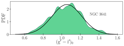
Figure 13: Smoothed colour distribution for GC candidates associated to NGC 3641. A black curve indicates the unimodal distribution resulting from the GMM fit.

4.3 Luminosity function

In Figure 14 we show the luminosity function of GC candidates associated to NGC 3641. We perform a similar analysis as with NGC 3640, performing the fit of a Gaussian function both using the turn-over from the literature (in this case, the same one as for NGC 3640), and then fitting our own value. We find an almost exact match, although our luminosity function is noisy, with a dispersion larger than usual ($0.9$), and showing bumps towards the brighter end which may be due to contamination from NGC 3640.

An integration of the luminosity function results in a total population of $\approx 135$ GC.

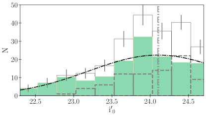
Figure 14: Luminosity function for the GC candidates associated to NGC 3641. Dashed green lines show the background distribution, black solid bars indicate the result from subtracting it from the raw distribution (green bars). The dot-dashed curve shows the Gaussian fit.

5 Spatial distribution and tidal features

The panels of Figure 15 show the contours of the spatial distribution of the GC candidates located across the field containing both galaxies, separated by colour, placing the limit in $(g^{\prime}-i^{\prime})=1$, drawn on top of residual images. These were obtained modelling both galaxies using the ELLIPSE task in iraf, and subtracting it from the image.

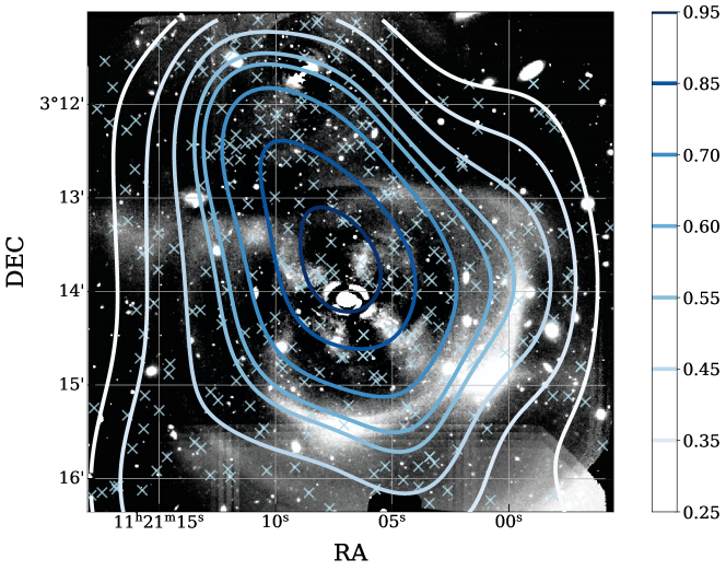
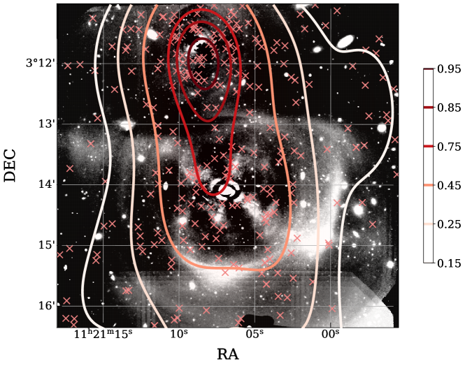
Figure 15: Smoothed distribution of GC candidates across the entire field separated between blue (top) and red (bottom), with density contours plotted in solid lines. Crosses in both panels show the individual positions, and the background is the residuals image of the field obtained in the $i^{\prime}$ filter after modelling both galaxies with the task ELLIPSE and subtracting them from the raw image.

In the top panel, we can see that the blue GCs are extended across the entire field. The contours follow one of the strongest substructures, identified by P88 as ‘A’. This behaviour may indicate that the interaction that caused the shell-like structure in ‘A’ also pushed the blue GCs in this direction.

The red GCs are more concentrated towards the region between both galaxies, and their density maps reveal a bridge that connects them. In combination with the overdensity in the colour distribution of NGC 3640 that matches the population of GCs associated to NGC 3641, this seems to indicate that NGC 3640 is accreting GCs from its neighbour, and this process is ongoing.

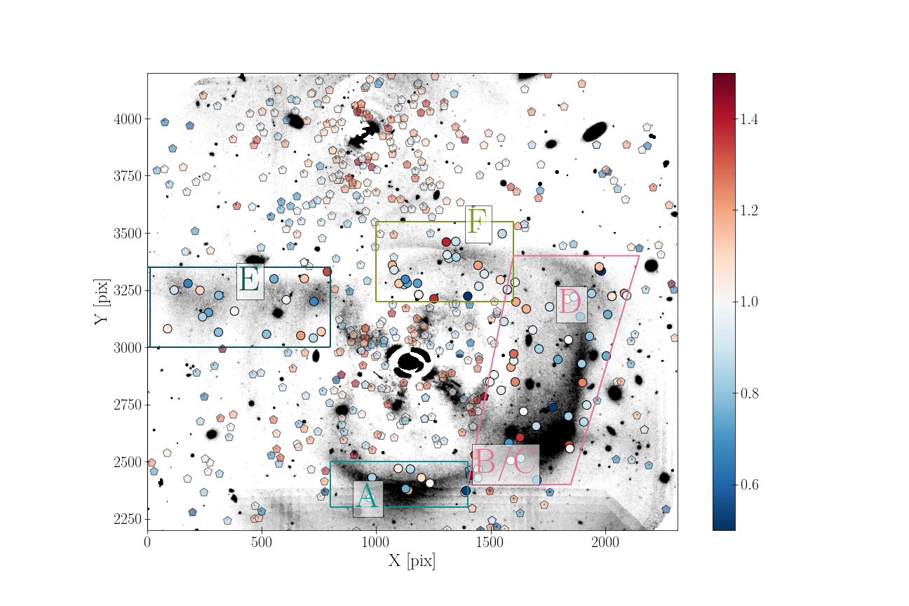
Figure 16: Image in the $i^{\prime}$ filter resulting from subtracting the model of the surface brightness profile of both galaxies. Circles indicate GC candidates across the entire field with their colours shown in a gradient, and polygons indicate the location of the shells following the nomenclature given in P88.

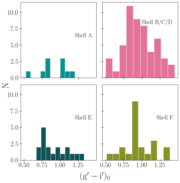
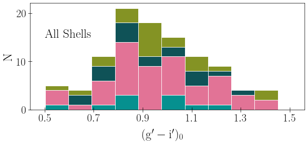
Figure 17: Histogram of GCs located in the regions defined as shells. Top image shows each shell separately, bottom one shows the combination of all the histograms, following the same color scheme as in the polygons in the previous Figure.

6 Discussion

6.1 GCs as tracers of substructures

In the current paradigm of ETG evolution, both major and minor mergers play important roles at different stages of galaxy evolution. Gas-rich major mergers dominate the early stages, while minor mergers become more relevant during the second phase of evolution, where ETGs grow their mass by accretion with very low to null rates of star formation (Oser et al., 2010; Naab et al., 2007; Hilz et al., 2012). These encounters leave traces behind as different types of substructures, e.g. streams, shells, tails, and plumes (Mancillas et al., 2019)[and references within]. We identify the substructures in NGC 3640 as shells since they are approximately semi-circular and concentric, mostly located on the northwest corner of the galaxy. Mancillas et al. (2019) attributes the fact that shells tend to accumulate on one side of the galaxy to the consequences of a satellite accretion event, where the arc is formed after the satellite falls into the central potential. In general, shells are expected to form after mergers with a 4:1 mass ratio at most, i.e. intermediate- to major-mass mergers (Pop et al., 2018; Karademir et al., 2019), and they survive around 4 Gyr. This upper limit for the timing of the accretion event is consistent with previous analyses of NGC 3640 which date the structures and parts of the stellar population (see Section 1).

The mergers the host galaxy undergoes shape the GCS. They may increase the population by either forming new GCs if there is enough gas involved and if the conditions are violent enough, or accreding old GCs from satellite galaxies. They may also alter their spatial distribution, redistributing them to the halo (Choksi & Gnedin, 2019; Dornan & Harris, 2023).

D’Abrusco et al. (2022) study statistically significant structures in the spatial distributions of the GCS of a variety of Fornax galaxies, concluding they are relics of accreted GC systems that are overlaid on the smooth distribution of the GCs belonging to the host galaxy. Following their analysis, we show in Figure 17 the colour distribution for the GCs that correspond spatially to the shells detected in the galaxy, identified in Figure 16. In shell F, located in the direction of NGC 3641, we find most GCs have a similar color, around $0.9$, bluer than those associated to NGC 3641. In substructures A and E, blue GCs dominate, while the region covered by substructure B/C/D has a wider color distribution, although it is also dominated by blue objects, including GCs with colors bluer than $0.7$.

This analysis is based on the distribution observed in 2D being representative of the physical position of the objects in the real, 3D Universe. D’Abrusco et al. (2022) argue that the risk of the 2D structures being merely projection effects is small. This is due to previous studies like Woodley & Harris (2011) showing through simulations that the probability of misidentifying a 2D subgroup is $1\%$, and to the fact that the identified structures present complex morphologies that a smooth 3D spatial distribution cannot explain.

6.2 Paucity of GCs in the inner region

The Hubble-Reynolds profile fit to the projected radial distribution of the GCS of NGC 3640 has a core radius of $r_{0}=1.16\,\textrm{arcmin}=9.07\,kpc$. Considering NGC 3640 has a stellar mass of $log{M_{\star}}=11.2$ (Karachentsev et al., 2015) we can place it in the context of the $r_{0}$ vs. $M_{\star}$ relation studied in Caso et al. (2024) for a sample of early-type galaxies in HST/ACS archival date. Given that Gemini data is not comparable in terms of depth with HST/ACS, even after a thorough completeness analysis, this number might be slightly enlarged in comparison to those in the sample in Caso et al. (2024). However, it is clear NGC 3640 has a larger core radius than most galaxies in the sample, especially for those with similar masses. This implies the GCS of NGC 3640 is flatter up to a larger galactocentric radius, which can also be seen by simple visual inspection of the projected spatial distribution in Figure 16, where the paucity of GCs near the centre of the galaxy is apparent.

The highest core radius value in the HST/ACS sample (Caso et al., 2024) corresponds to NGC 4406 (M86), a galaxy that presents an offset peak in its GCS connected to a potential disturbance caused by a satellite dwarf galaxy, and a shell that is both seen in the low-surface brightness analysis (Mihos et al., 2017) and the GC spatial structure (Lambert et al., 2020). The two following galaxies are NGC 1316 and NGC 4472 (M49), both having undergone late, major mergers. Numerical simulations of hierarchical galaxy formation including GCs have shown that mergers or large accretion events such as being tidally stripped are the most frequent causes of GCs being redistributed to the halo (Kravtsov & Gnedin, 2005; Kruijssen & Cooper, 2012; Rieder et al., 2013). Using the E-MOSAICS suite of cosmological simulations, Kruijssen (2015) and more recently Keller et al. (2020) have both shown that mergers play a vital role in the survival of GCs since they eject them to the outskirts where the interstellar medium is less dense and they are less prone to experience tidal shocks.

It follows then that the connection between lower values of core radius for the GCS and galaxies that show substructures that imply major mergers not long in the past is a physical one. Large accretion events directly affect the radial distribution of GCs, not so much through the creation of young GCs but through the flattening of the inner region due to redistribution. In Table 3, we show that the red fraction increases as we move away from the central region. In the current paradigm of GC formation, blue GCs are expected to dominate in the outer region since a large fraction of them comes from accretion of satellite galaxies, while most red GCs are thought to have formed in-situ. This difference can be interpreted as a sign of redistribution mechanisms at play.

6.3 The bridge?

The possibility of NGC 3640 and NGC 3641 interacting is not discussed in previous work, mainly due to the observations focusing on the central regions NGC 3640. In terms of integrated light, we do not detect a significant overdensity that can be interpreted as a stream between the two, but it could potentially be fainter than our magnitude limit. Since GCs have been shown to trace stellar streams (Blom et al., 2014; Napolitano et al., 2022, e.g.), it is reasonable to interpret the overdensity detected between the two galaxies as a hint that there might be a stream between them. Previous works in other galaxies have also found potential bridges made of GCs as tracers of interactions, such as Bassino et al. (2006) connecting NGC 1387 and NGC 1399, and Wehner et al. (2008) with NGC 3311 and NGC 3309. We see that the colours of the GCs spatially situated between both galaxies are mainly intermediate, closer to the peak of the population associated with NGC 3641, perhaps due to being members of its GCS that are being accreted by the more massive galaxy. As is originally mentioned in P88, the compactness of NGC 3641 implies a high angular momentum interaction. Although they refrain from interpreting anything more conclusive, they point out that the dust lane in NGC 3640 is oriented in the direction of its neighbour, which is encouraging.

Solid evidence of the interaction can only be obtained through spectroscopy, which would allow us to confirm membership of the GCs as well as to analyze their kinematics, which might confirm the connection between the two galaxies.

7 Conclusions

We perform a wide-field photometric study of the GCS of NGC 3640 and NGC 3641, using data obtained from GMOS/Gemini. We attribute GCs to the GCS of each galaxy based on projected distance, and analyze each of them separately. NGC 3640 presents a bimodal GCS, with blue GCs that extend towards the outer regions of the field, and red GCs concentrated towards the centre. The luminosity function allows us to estimate a total population of $\approx 350$ GCs. In NGC 3641 we find a unimodal distribution, with GCs in an intermediate colour range in relation to the subpopulations in NGC 3640.

Finally, we identify a potential connection between the spatial distribution of the GCs and the shell-like structures around NGC 3640, which hints at a major merger having disrupted the GCS. We also indicate the potential presence of a bridge formed by red GCs that connect both galaxies, indicating they may be currently interacting. Further spectroscopic studies are necessary to solidify these claims.

References

- Astropy Collaboration et al. (2013) Astropy Collaboration et al., 2013, \hrefhttp://dx.doi.org/10.1051/0004-6361/201322068 A&A, \hrefhttp://adsabs.harvard.edu/abs/2013A
- Astropy Collaboration et al. (2018) Astropy Collaboration et al., 2018, \hrefhttp://dx.doi.org/10.3847/1538-3881/aabc4f AJ, \hrefhttps://ui.adsabs.harvard.edu/abs/2018AJ….156..123A 156, 123
- Astropy Collaboration et al. (2022) Astropy Collaboration et al., 2022, \hrefhttp://dx.doi.org/10.3847/1538-4357/ac7c74 ApJ, \hrefhttps://ui.adsabs.harvard.edu/abs/2022ApJ…935..167A 935, 167
- Bassino & Caso (2017) Bassino L. P., Caso J. P., 2017, \hrefhttp://dx.doi.org/10.1093/mnras/stw3390 MNRAS, \hrefhttps://ui.adsabs.harvard.edu/abs/2017MNRAS.466.4259B 466, 4259
- Bassino et al. (2006) Bassino L. P., Richtler T., Dirsch B., 2006, \hrefhttp://dx.doi.org/10.1111/j.1365-2966.2005.09919.x MNRAS, \hrefhttps://ui.adsabs.harvard.edu/abs/2006MNRAS.367..156B 367, 156
- Bender et al. (1988) Bender R., Doebereiner S., Moellenhoff C., 1988, A&AS, \hrefhttps://ui.adsabs.harvard.edu/abs/1988A&AS…74..385B 74, 385
- Bertin & Arnouts (1996) Bertin E., Arnouts S., 1996, \hrefhttp://dx.doi.org/10.1051/aas:1996164 A&AS, \hrefhttps://ui.adsabs.harvard.edu/abs/1996A&AS..117..393B 117, 393
- Blom et al. (2014) Blom C., Forbes D. A., Foster C., Romanowsky A. J., Brodie J. P., 2014, \hrefhttp://dx.doi.org/10.1093/mnras/stu095 MNRAS, \hrefhttps://ui.adsabs.harvard.edu/abs/2014MNRAS.439.2420B 439, 2420
- Blumenthal et al. (1984) Blumenthal G. R., Faber S. M., Primack J. R., Rees M. J., 1984, \hrefhttp://dx.doi.org/10.1038/311517a0 Nature, \hrefhttps://ui.adsabs.harvard.edu/abs/1984Natur.311..517B 311, 517
- Bradley et al. (2023) Bradley L., et al., 2023, astropy/photutils: 1.8.0, \hrefhttp://dx.doi.org/10.5281/zenodo.7946442 doi:10.5281/zenodo.7946442, \urlhttps://doi.org/10.5281/zenodo.7946442
- Brough et al. (2007) Brough S., Proctor R., Forbes D. A., Couch W. J., Collins C. A., Burke D. J., Mann R. G., 2007, \hrefhttp://dx.doi.org/10.1111/j.1365-2966.2007.11900.x MNRAS, \hrefhttps://ui.adsabs.harvard.edu/abs/2007MNRAS.378.1507B 378, 1507
- Caso et al. (2019) Caso J. P., De Bórtoli B. J., Ennis A. I., Bassino L. P., 2019, \hrefhttp://dx.doi.org/10.1093/mnras/stz2039 MNRAS, \hrefhttps://ui.adsabs.harvard.edu/abs/2019MNRAS.488.4504C 488, 4504
- Caso et al. (2024) Caso J. P., Ennis A. I., De Bórtoli B. J., 2024, \hrefhttp://dx.doi.org/10.1093/mnras/stad3602 MNRAS, \hrefhttps://ui.adsabs.harvard.edu/abs/2024MNRAS.527.6993C 527, 6993
- Choksi & Gnedin (2019) Choksi N., Gnedin O. Y., 2019, \hrefhttp://dx.doi.org/10.1093/mnras/stz2097 MNRAS, \hrefhttps://ui.adsabs.harvard.edu/abs/2019MNRAS.488.5409C 488, 5409
- D’Abrusco et al. (2022) D’Abrusco R., Zegeye D., Fabbiano G., Cantiello M., Paolillo M., Zezas A., 2022, \hrefhttp://dx.doi.org/10.3847/1538-4357/ac4be2 ApJ, \hrefhttps://ui.adsabs.harvard.edu/abs/2022ApJ…927…15D 927, 15
- Davis et al. (1985) Davis M., Efstathiou G., Frenk C. S., White S. D. M., 1985, \hrefhttp://dx.doi.org/10.1086/163168 ApJ, \hrefhttps://ui.adsabs.harvard.edu/abs/1985ApJ…292..371D 292, 371
- Denicoló et al. (2005) Denicoló G., Terlevich R., Terlevich E., Forbes D. A., Terlevich A., 2005, \hrefhttp://dx.doi.org/10.1111/j.1365-2966.2005.08748.x MNRAS, \hrefhttps://ui.adsabs.harvard.edu/abs/2005MNRAS.358..813D 358, 813
- Dornan & Harris (2023) Dornan V., Harris W. E., 2023, \hrefhttp://dx.doi.org/10.3847/1538-4357/accbc3 ApJ, \hrefhttps://ui.adsabs.harvard.edu/abs/2023ApJ…950..179D 950, 179
- Ellison et al. (2011) Ellison S. L., Patton D. R., Mendel J. T., Scudder J. M., 2011, \hrefhttp://dx.doi.org/10.1111/j.1365-2966.2011.19624.x MNRAS, \hrefhttps://ui.adsabs.harvard.edu/abs/2011MNRAS.418.2043E 418, 2043
- Etherington et al. (2017) Etherington J., et al., 2017, MNRAS, 466
- Faifer et al. (2011) Faifer F. R., et al., 2011, \hrefhttp://dx.doi.org/10.1111/j.1365-2966.2011.19018.x MNRAS, \hrefhttps://ui.adsabs.harvard.edu/abs/2011MNRAS.416..155F 416, 155
- Forbes et al. (2011) Forbes D. A., Spitler L. R., Strader J., Romanowsky A. J., Brodie J. P., Foster C., 2011, \hrefhttp://dx.doi.org/10.1111/j.1365-2966.2011.18373.x MNRAS, \hrefhttps://ui.adsabs.harvard.edu/abs/2011MNRAS.413.2943F 413, 2943
- Harris et al. (2009) Harris W. E., Kavelaars J. J., Hanes D. A., Pritchet C. J., Baum W. A., 2009, \hrefhttp://dx.doi.org/10.1088/0004-6256/137/2/3314 AJ, \hrefhttps://ui.adsabs.harvard.edu/abs/2009AJ….137.3314H 137, 3314
- Harris et al. (2014) Harris W. E., et al., 2014, \hrefhttp://dx.doi.org/10.1088/0004-637X/797/2/128 ApJ, \hrefhttps://ui.adsabs.harvard.edu/abs/2014ApJ…797..128H 797, 128
- Harris et al. (2020) Harris C. R., et al., 2020, \hrefhttp://dx.doi.org/10.1038/s41586-020-2649-2 Nature, 585, 357
- Hilz et al. (2012) Hilz M., Naab T., Ostriker J. P., Thomas J., Burkert A., Jesseit R., 2012, \hrefhttp://dx.doi.org/10.1111/j.1365-2966.2012.21541.x MNRAS, \hrefhttps://ui.adsabs.harvard.edu/abs/2012MNRAS.425.3119H 425, 3119
- Hopkins et al. (2010) Hopkins P. F., et al., 2010, \hrefhttp://dx.doi.org/10.1088/0004-637X/724/2/915 ApJ, \hrefhttps://ui.adsabs.harvard.edu/abs/2010ApJ…724..915H 724, 915
- Hunter (2007) Hunter J. D., 2007, \hrefhttp://dx.doi.org/10.1109/MCSE.2007.55 Computing in Science & Engineering, 9, 90
- Jørgensen (2009) Jørgensen I., 2009, \hrefhttp://dx.doi.org/10.1071/AS08008 PASA, \hrefhttps://ui.adsabs.harvard.edu/abs/2009PASA…26…17J 26, 17
- Kannan et al. (2015) Kannan R., Macciò A. V., Fontanot F., Moster B. P., Karman W., Somerville R. S., 2015, \hrefhttp://dx.doi.org/10.1093/mnras/stv1633 MNRAS, \hrefhttps://ui.adsabs.harvard.edu/abs/2015MNRAS.452.4347K 452, 4347
- Karachentsev et al. (2015) Karachentsev I. D., Nasonova O. G., Karachentseva V. E., 2015, \hrefhttp://dx.doi.org/10.1134/S1990341315010010 Astrophysical Bulletin, \hrefhttps://ui.adsabs.harvard.edu/abs/2015AstBu..70….1K 70, 1
- Karademir et al. (2019) Karademir G. S., Remus R.-S., Burkert A., Dolag K., Hoffmann T. L., Moster B. P., Steinwandel U. P., Zhang J., 2019, \hrefhttp://dx.doi.org/10.1093/mnras/stz1251 MNRAS, \hrefhttps://ui.adsabs.harvard.edu/abs/2019MNRAS.487..318K 487, 318
- Kaviraj et al. (2011) Kaviraj S., Tan K.-M., Ellis R. S., Silk J., 2011, \hrefhttp://dx.doi.org/10.1111/j.1365-2966.2010.17754.x MNRAS, \hrefhttps://ui.adsabs.harvard.edu/abs/2011MNRAS.411.2148K 411, 2148
- Keller et al. (2020) Keller B. W., Kruijssen J. M. D., Pfeffer J., Reina-Campos M., Bastian N., Trujillo-Gomez S., Hughes M. E., Crain R. A., 2020, \hrefhttp://dx.doi.org/10.1093/mnras/staa1439 MNRAS, \hrefhttps://ui.adsabs.harvard.edu/abs/2020MNRAS.495.4248K 495, 4248
- Kormendy (1982) Kormendy J., 1982, Saas-Fee Advanced Course, \hrefhttps://ui.adsabs.harvard.edu/abs/1982SAAS…12..115K 12, 115
- Kravtsov & Gnedin (2005) Kravtsov A. V., Gnedin O. Y., 2005, \hrefhttp://dx.doi.org/10.1086/428636 ApJ, \hrefhttps://ui.adsabs.harvard.edu/abs/2005ApJ…623..650K 623, 650
- Kruijssen (2015) Kruijssen J. M. D., 2015, \hrefhttp://dx.doi.org/10.1093/mnras/stv2026 MNRAS, \hrefhttps://ui.adsabs.harvard.edu/abs/2015MNRAS.454.1658K 454, 1658
- Kruijssen & Cooper (2012) Kruijssen J. M. D., Cooper A. P., 2012, \hrefhttp://dx.doi.org/10.1111/j.1365-2966.2011.20037.x MNRAS, \hrefhttps://ui.adsabs.harvard.edu/abs/2012MNRAS.420..340K 420, 340
- Labrie et al. (2019) Labrie K., Anderson K., Cárdenes R., Simpson C., Turner J. E. H., 2019, in Teuben P. J., Pound M. W., Thomas B. A., Warner E. M., eds, Astronomical Society of the Pacific Conference Series Vol. 523, Astronomical Data Analysis Software and Systems XXVII. p. 321
- Lambert et al. (2020) Lambert R. A., Rhode K. L., Vesperini E., 2020, \hrefhttp://dx.doi.org/10.3847/1538-4357/abaab2 ApJ, \hrefhttps://ui.adsabs.harvard.edu/abs/2020ApJ…900…45L 900, 45
- Landolt (1992) Landolt A. U., 1992, \hrefhttp://dx.doi.org/10.1086/116242 AJ, \hrefhttps://ui.adsabs.harvard.edu/abs/1992AJ….104..340L 104, 340
- Lim et al. (2017) Lim S., et al., 2017, \hrefhttp://dx.doi.org/10.3847/1538-4357/835/2/123 ApJ, \hrefhttps://ui.adsabs.harvard.edu/abs/2017ApJ…835..123L 835, 123
- Madore et al. (2004) Madore B. F., Freedman W. L., Bothun G. D., 2004, \hrefhttp://dx.doi.org/10.1086/383486 ApJ, \hrefhttps://ui.adsabs.harvard.edu/abs/2004ApJ…607..810M 607, 810
- Mancillas et al. (2019) Mancillas B., Duc P.-A., Combes F., Bournaud F., Emsellem E., Martig M., Michel-Dansac L., 2019, \hrefhttp://dx.doi.org/10.1051/0004-6361/201936320 A&A, \hrefhttps://ui.adsabs.harvard.edu/abs/2019A&A…632A.122M 632, A122
- McKinney (2010) McKinney W., 2010, in van der Walt S., Millman J., eds, Proceedings of the 9th Python in Science Conference. pp 51 – 56
- McNaught-Roberts et al. (2014) McNaught-Roberts T., et al., 2014, \hrefhttp://dx.doi.org/10.1093/mnras/stu1886 MNRAS, \hrefhttps://ui.adsabs.harvard.edu/abs/2014MNRAS.445.2125M 445, 2125
- Michard & Prugniel (2004) Michard R., Prugniel P., 2004, \hrefhttp://dx.doi.org/10.1051/0004-6361:20035637 A&A, \hrefhttps://ui.adsabs.harvard.edu/abs/2004A&A…423..833M 423, 833
- Mihos et al. (2017) Mihos J. C., Harding P., Feldmeier J. J., Rudick C., Janowiecki S., Morrison H., Slater C., Watkins A., 2017, \hrefhttp://dx.doi.org/10.3847/1538-4357/834/1/16 ApJ, \hrefhttps://ui.adsabs.harvard.edu/abs/2017ApJ…834…16M 834, 16
- Muratov & Gnedin (2010) Muratov A. L., Gnedin O. Y., 2010, \hrefhttp://dx.doi.org/10.1088/0004-637X/718/2/1266 ApJ, \hrefhttps://ui.adsabs.harvard.edu/abs/2010ApJ…718.1266M 718, 1266
- Naab et al. (2007) Naab T., Johansson P. H., Ostriker J. P., Efstathiou G., 2007, \hrefhttp://dx.doi.org/10.1086/510841 ApJ, \hrefhttps://ui.adsabs.harvard.edu/abs/2007ApJ…658..710N 658, 710
- Naab et al. (2009) Naab T., Johansson P. H., Ostriker J. P., 2009, \hrefhttp://dx.doi.org/10.1088/0004-637X/699/2/L178 ApJ, \hrefhttps://ui.adsabs.harvard.edu/abs/2009ApJ…699L.178N 699, L178
- Napolitano et al. (2022) Napolitano N. R., et al., 2022, \hrefhttp://dx.doi.org/10.1051/0004-6361/202141872 A&A, \hrefhttps://ui.adsabs.harvard.edu/abs/2022A&A…657A..94N 657, A94
- Oser et al. (2010) Oser L., Ostriker J. P., Naab T., Johansson P. H., Burkert A., 2010, \hrefhttp://dx.doi.org/10.1088/0004-637X/725/2/2312 ApJ, \hrefhttps://ui.adsabs.harvard.edu/abs/2010ApJ…725.2312O 725, 2312
- Osmond & Ponman (2004) Osmond J. P. F., Ponman T. J., 2004, in Mulchaey J. S., Dressler A., Oemler A., eds, Clusters of Galaxies: Probes of Cosmological Structure and Galaxy Evolution. p. 39
- Pedregosa et al. (2011) Pedregosa F., et al., 2011, Journal of Machine Learning Research, 12, 2825
- Peebles (1982) Peebles P. J. E., 1982, \hrefhttp://dx.doi.org/10.1086/183911 ApJ, \hrefhttps://ui.adsabs.harvard.edu/abs/1982ApJ…263L…1P 263, L1
- Pop et al. (2018) Pop A.-R., Pillepich A., Amorisco N. C., Hernquist L., 2018, \hrefhttp://dx.doi.org/10.1093/mnras/sty1932 MNRAS, \hrefhttps://ui.adsabs.harvard.edu/abs/2018MNRAS.480.1715P 480, 1715
- Prugniel et al. (1988) Prugniel P., Nieto J. L., Bender R., Davoust E., 1988, A&A, \hrefhttps://ui.adsabs.harvard.edu/abs/1988A&A…204…61P 204, 61
- Rieder et al. (2013) Rieder S., Ishiyama T., Langelaan P., Makino J., McMillan S. L. W., Portegies Zwart S., 2013, \hrefhttp://dx.doi.org/10.1093/mnras/stt1848 MNRAS, \hrefhttps://ui.adsabs.harvard.edu/abs/2013MNRAS.436.3695R 436, 3695
- Satyapal et al. (2014) Satyapal S., Ellison S. L., McAlpine W., Hickox R. C., Patton D. R., Mendel J. T., 2014, \hrefhttp://dx.doi.org/10.1093/mnras/stu650 MNRAS, \hrefhttps://ui.adsabs.harvard.edu/abs/2014MNRAS.441.1297S 441, 1297
- Schweizer & Seitzer (1992) Schweizer F., Seitzer P., 1992, \hrefhttp://dx.doi.org/10.1086/116296 AJ, \hrefhttps://ui.adsabs.harvard.edu/abs/1992AJ….104.1039S 104, 1039
- Sesto et al. (2016) Sesto L. A., Faifer F. R., Forte J. C., 2016, \hrefhttp://dx.doi.org/10.1093/mnras/stw1627 MNRAS, \hrefhttps://ui.adsabs.harvard.edu/abs/2016MNRAS.461.4260S 461, 4260
- Strader et al. (2004) Strader J., Brodie J. P., Forbes D. A., 2004, \hrefhttp://dx.doi.org/10.1086/380614 AJ, \hrefhttps://ui.adsabs.harvard.edu/abs/2004AJ….127..295S 127, 295
- Tal et al. (2009) Tal T., van Dokkum P. G., Nelan J., Bezanson R., 2009, \hrefhttp://dx.doi.org/10.1088/0004-6256/138/5/1417 AJ, \hrefhttps://ui.adsabs.harvard.edu/abs/2009AJ….138.1417T 138, 1417
- Tully et al. (2013) Tully R. B., et al., 2013, \hrefhttp://dx.doi.org/10.1088/0004-6256/146/4/86 AJ, \hrefhttps://ui.adsabs.harvard.edu/abs/2013AJ….146…86T 146, 86
- Virtanen et al. (2020) Virtanen P., et al., 2020, \hrefhttp://dx.doi.org/10.1038/s41592-019-0686-2 Nature Methods, \hrefhttps://rdcu.be/b08Wh 17, 261
- Wehner et al. (2008) Wehner E. M. H., Harris W. E., Whitmore B. C., Rothberg B., Woodley K. A., 2008, \hrefhttp://dx.doi.org/10.1086/587433 ApJ, \hrefhttps://ui.adsabs.harvard.edu/abs/2008ApJ…681.1233W 681, 1233
- Woodley & Harris (2011) Woodley K. A., Harris W. E., 2011, \hrefhttp://dx.doi.org/10.1088/0004-6256/141/1/27 AJ, \hrefhttps://ui.adsabs.harvard.edu/abs/2011AJ….141…27W 141, 27
- Woodley et al. (2010) Woodley K. A., Harris W. E., Puzia T. H., Gómez M., Harris G. L. H., Geisler D., 2010, \hrefhttp://dx.doi.org/10.1088/0004-637X/708/2/1335 ApJ, \hrefhttps://ui.adsabs.harvard.edu/abs/2010ApJ…708.1335W 708, 1335
- de Vaucouleurs et al. (1976) de Vaucouleurs G., de Vaucouleurs A., Corwin H. G., 1976, 2nd reference catalogue of bright galaxies containing information on 4364 galaxies with reference to papers published between 1964 and 1975
- de Vaucouleurs et al. (1991) de Vaucouleurs G., de Vaucouleurs A., Corwin Herold G. J., Buta R. J., Paturel G., Fouque P., 1991, Third Reference Catalogue of Bright Galaxies