Strong non-linear response of strange metals

Abstract

Understanding the behavior and properties of strange metals remains an outstanding challenge in correlated electron systems. Recently, a model of a quantum critical metal with spatially random couplings to a critical boson (Patel et al., Science 381, 790 (2023)) has been shown to capture the linear-in-$T$ resistivity down to zero temperature ($T$) - one of the universal experimental signatures of strange metals. In our work we explore the non-linear transport properties of such a model of strange metal. Uniting the large-$N$ and Keldysh field theory formalisms, we derive a set of kinetic equations for the strange metal and use it to compute nonlinear conductivity. We find that the third-order conductivity is enhanced by a factor of ${T_{F}}/{T}$ in comparison to a Fermi liquid, resulting in a strong temperature dependence. This behavior is shown to arise from the strong, non-analytic energy dependence of scattering rate and self-energies for electrons. We highlight the role of energy relaxation and electron-boson drag for the nonlinear responses. Finally, we discuss the potential for nonanalytic nonlinear electric field ($\mathbf{E}$) response arising at low temperatures. Our work demonstrates the characteristic features of strange metals in nonlinear transport, that may allow to gain more insight about their behavior in future experiments.

I Introduction

The strange metal state remains one of the most enigmatic phenomena in correlated electron systems, where both its microscopic origin and definitive set of characteristic behaviors remain under debate, calling for new probes and theoretical predictions. Recent advances in THz optics have opened the way to probe nonlinear transport properties of correlated electronic systems. So far, these techniques have found applications in probing collective modes in superconductors [1, 2, 3, 4], quantum spin systems [5, 6, 7, 8] and strongly disordered semiconductors [9]. There, useful analogies with two-level systems can often be established [9], allowing to characterize and classify the relevant relaxation processes. A large body of work also exists on nonlinear transport effect in semiconductors [10, 11, 12], where features of the band structure and impurity scattering are intimately related to the nonlinear response, best represented by the strong response of Dirac systems. In weakly interacting metals, nonlinear effects appear due to the band non-parabolicity and are expected to be small due to large Fermi energy [make more precise?]. However, the potential influence of strong correlations have not been up to date theoretically investigated, while recent experiments demonstrate the feasibility of such measurements [13] .

In this work we show that strange metals possess a strong nonlinear conductivity response in contrast to Fermi-liquid metals. This behavior arises from the $\sim\omega$ energy-dependent scattering, and thus constitutes a new ”defining property” of the strange metal state, along with linear-in-$T$ resistivity and thermodynamic scaling. We also show the appearance of a scaling relation between voltage and temperature at low temperature, which has some similarities to that found near quantum critical points of bosons [14, 15, 16, 17, 18].

To describe the strange metal, we will use the microscopic model recently put forward capturing one of the ”trademark” strange metal behaviors : resistivity following a linear temperature dependence $\rho\sim T$ down to zero.

The model was originally developed in the series of works [19, 20, 21, 22, 23, 24] and is an SYK-type model of a fermionic mode coupled to a scalar boson in the vicinity of a QCP in two spatial dimensions, building upon earlier work on the zero-dimensional Yukawa-SYK model [25, 26, 27, 28, 29, 30]. A particular feature of the model that allows to reproduce the Plankian scattering rate comes in a form a spatially disordered coupling between the fields and potential disorder, so called $v-g\prime$ model. In this work we assume that fermion dispersion is linearized in the vicinity of the Fermi surface and adopt a minimal coupling to the electric field. We use Keldysh field theory combined with the $\Sigma-G$ effective action method to derive quasiclassical kinetic equations for both fermionic and bosonic fields as self-consistent dynamic degrees of freedom. In particular, our method allows us to obtain the results without the typical assumption of a boson being in thermal equilibrium. As a side result, we show that when the boson dynamics is being accounted for, the bosonic degrees of freedom no longer play a role of a thermal bath and the total energy of the system is conserved. The energy conservation in this model of strange metals is a consequence of absence of any coupling to an external thermal bath or an outside field that could serve as an energy drain. Our method allows us to study the boson and fermion dynamics and prove the energy conservation even with disorder present at the level of kinetic equations.

As a main result of the paper, we present a study of third order electrical response of the aforementioned model and compute the non-linear third order conductivity. We find that some non-linear responses arise due to two expected mechanisms: dynamics of higher angular momentum harmonics and dynamics of the energy density harmonic. We classify those two types of responses as “ordinary” non-linear response and the “Joule-heating” response correspondingly. We discriminate two types of terms due to a special role of the energy relaxation in the responses to spatially uniform perturbations. In the presence of spatial modulation of the source field the energy relaxation is often greatly enhanced due to the interplay of screening effects and charge density redistribution in the material. With that motivation, we showcase the structure of both the term that comes from the “heating” of the system, and from the proper non-linearity in the system to highlight that further study of the energy relaxation mechanisms in strange metals is necessary.

We show that at low temperatures both Joule heating type and ordinary type of third order response are enhanced by a factor of $T_{F}/T$ in comparison to the analogous response that would have been expected in a Fermi liquid state with similar Fermi surface parameters ($\varepsilon_{F}$ - Fermi energy), which is schematically shown in Fig. 1. Additionally, we conjecture the structure of the Joule heating and ordinary non-linear responses at all orders of perturbation theory and show that the ordinary non-linear response is exhibits a universal $|\mathbf{E}|/T$ scaling ($\mathbf{E}$ - electric field), while the scaling of the Joule heating non-linear response strongly depends on the energy relaxation mechanism in a real system. However, in the optical regime, when we can neglect the energy relaxation processes in the system and treat the system as closed, we show that the non-linear response exhibits universal scaling $|\mathbf{E}|/T\sqrt{\nu}$, where $\nu$ is a frequency of the external field. In the regime of low frequencies the energy relaxation rate becomes dominant and thus is above this paper scope and is a subject of a future study.

The rest of the paper is structured as follows. In the end of the current section (Sec. I) we provide a brief summary of the main results and compare the non-linear responses in the considered model of strange metal with expected results for a Fermi liquid. In Section II we describe in details the model that we employ to study the strange metal phase and upgrade it to the form suitable for the Keldysh field theory [31] calculation. In Section III we convert the theory into Keldysh formalism and employ $G-\Sigma$ effective action method with large-$N$ expansion to derive the set of equations that connect Keldysh-Green functions and self-energies. In Section IV we present a quasi-classical limit of Keldysh kinetic equations that govern the dynamics of both fermions and bosons in a self-consistent manner. In Section V we explore the properties of the energy relaxation in the given model, showcase the energy conservation in the closed system, and discuss the limitations of the model. In Section VI we construct the perturbative solution to the Keldysh kinetic equations obtained in Sec. IV and compute the non-linear conductivity responses.

I.1 Summary of results and comparison to Fermi liquids

We highlight the results of our non-linear response calculation in the strange metal phase and compare them to the corresponding non-linear responses in Fermi liquids. A typical kinetic equation for a Fermi-liquid distribution function when homogeneous electric field $\mathbf{E}(t)$ is applied can be written as

$$a\,\partial_{t}\delta f+ev_{F}(\hat{\mathbf{k}}\cdot\mathbf{E})\,\partial_{\omega}(\bar{f}+\delta f)=I[\delta f],$$ (1)

where $\delta f(t,\omega,\hat{\mathbf{k}})=f(t,\omega,\hat{\mathbf{k}})-\bar{f}(\omega)$ is a perturbation of the distribution function away from the equilibrium, $\omega$ is an energy of the Landau quasi-particle, and $\hat{\mathbf{k}}$ is a unit vector marking direction on the Fermi-surface. The constant $a$ is a dimensionless constant that represents the renormalized by the interaction dynamic term, $v_{F}$ is a Fermi-velocity and is related to the inverse effective mass. In this paper we show that the strange metal dynamics is governed by a kinetic equation of a form similar to Eq. (1), even though the Landau quasiparticles are absent and the excitations experience strong mutual drag. Such kinetic equation originates from Keldysh field theory, where energy $\omega$ and the distribution function $f(\omega)$ preserve their meaning of the excitation energy and distribution function correspondingly, as long as the relevant Green’s functions are still sharp functions of momentum around fermi momentum $k_{F}$ [32]. The main difference between strange metals and Fermi liquids comes in the structure of the collision integral $I$ in Eq. (1).

Assuming rotational symmetry, the structure of the collision integral in a typical Fermi-liquid can be conveniently described by expanding the perturbation $\delta f$ into angular harmonics: $\delta f=\sum\delta f_{m}e^{im\theta_{\hat{\mathbf{k}}}}$. The simplest structure the collision integral takes a form

$$I_{\mathrm{FL}}[\delta f]=-\sum_{m}\gamma_{\mathrm{FL,}m}\delta f_{m}e^{im\theta_{\hat{\mathbf{k}}}},$$ (2)

when in case $m\neq 0$ rates $\gamma_{\mathrm{FL,}m}=\Gamma+\gamma_{\mathrm{FL}}(\pi^{2}T^{2}+\omega^{2})/\varepsilon_{F}$ with $\varepsilon_{F}$ being the Fermi-energy, and $\gamma_{\mathrm{FL}}$ is a dimensionless constant of the order of unity ($k_{B}=\hbar=1$). The constant contribution $\Gamma$ comes from the elastic collision disorder. This behavior of $\gamma_{\mathrm{FL,}m}$ is a typical $\sim\omega^{2}$ and $\sim T^{2}$ behavior in Fermi liquids.

We derive the structure of strange metals collision integral, which can be also written as

$$I_{\mathrm{nFL}}[\delta f]=-\sum_{m}\gamma_{\mathrm{nFL},m}\delta f_{m}e^{im\theta_{\hat{\mathbf{k}}}}$$ (3)

up to non linear corrections, which end up having no qualitative effects, but are still included in the calculation. Additional feature of the strange metal that we obtain is a logarithmic divergence of a dynamics coefficient $a\sim\log 1/T$.

The main difference between the Fermi liquid and strange metal collision integral comes from the structure of $\omega$-dependence of the decay rates in both of the theories. We show that the strange metal decay rates are only functions of $T$ and $\omega/T$, which is significantly different from the Fermi liquids, where the characteristic scale for frequency is suppressed by $\varepsilon_{F}$.

The feature of $\omega/T$ dependence appears from the structure of the fermion self-energy, since in Keldysh field theory $\gamma_{\mathrm{nFL}}\sim\,\mathrm{Im}\,\Sigma_{R}$, where $\Sigma_{R}=\Sigma_{R}(\omega/T,T)$ is a retarded fermion self energy.We showcase below that such $\omega/T$ dependence is a crucial ingredient for strong non-linear responses, since it changes the non-linearity scaling from $1/\varepsilon_{F}$ to $1/T$, which is an enhancement by a $T_{F}/T$ at every order. This feature is expected to be generic in models with$\omega/T$ self-energy dependence, leading to a similar enhancement of non-linear responses.

The relaxation rate $\gamma_{\mathrm{FL,}0}=\Gamma_{0}(T)$ of the density harmonic $m=0$ is rather more special, since the relaxation rate of the density is related to different mechanisms of the energy drain in the system that is beyond the phenomenology of both Fermi liquid and strange metal. For example, in a closed system it is expected that $\Gamma_{0}=0$, in the case of coupling to the thermalized phonon bath $\Gamma_{0}=1/\tau_{\mathrm{el-ph}}\sim T$ above the Bloch-Gruneisen temperature [33] and $\Gamma_{0}\sim T^{4}$ below it. The energy relaxation rate in strange metals, on the other side, is much less understood. In our model we considered two phenomenological limits. First limit is a regime of closed system, which is relevant when the timescale of the evolution is much smaller then the timescale of the energy relaxation. We show that in lowest orders of response such model leads to $\gamma_{\mathrm{nFL,}0}=\Gamma_{0}\sim 0$, reflecting energy conservation in the system. Another limit corresponds to the regime of suppressed boson dynamics due to an interaction with an external heat bath. We show that this would lead to a relaxation rate $\Gamma_{0}\sim T$ at all the temperature scales.

One can solve the kinetic equation in Eq. (1) with collision rates for Fermi-liquids and extract in the linear order well known result for the linear resistivity $\rho_{\mathrm{FL}}(T)$:

$$\frac{1}{\sigma_{\mathrm{FL}}(T,\nu)}=\rho_{\mathrm{FL}}(T,\nu)=\rho_{0}+i\nu\,\beta_{\rho,\mathrm{FL}}+\kappa_{\rho}T^{2},$$ (4)

where the term $\rho_{0}$ comes from disorder, and coefficients $\rho_{\mathrm{FL},\nu}$ and $\rho_{\mathrm{nFL},T}$ are in the linear order independent from frequency and temperature constants defined only by the parameters of the Fermi surface: $\beta_{\rho,\mathrm{FL}}=2\pi\hbar a/e^{2}k_{F}v_{F}$, $\kappa_{\rho}=8\pi^{3}\gamma_{\mathrm{FL}}(\Delta)/3e^{2}k_{F}v_{F}\varepsilon_{F}$ ($k_{B}=1$). The unitless value $\gamma_{\mathrm{FL}}(\Delta)\sim 1$ away from the QCP, and grows in the vicinity of QCP, which is discussed below Eq. (10). As a side result of our calculation we re-derive the linear 1-sheet resistivity of the strange metals in the scope of the considered model and obtain linear in $T$ resistivity (up to a double-log of $1/T$):

$$\rho_{\mathrm{nFL}}(\nu,T)=\frac{1}{\sigma_{\mathrm{nFL}}(\nu,T)}=\rho_{0}+i\nu\beta_{\rho}\ln\left(\frac{T_{\Lambda}}{T}\right)+\alpha_{\rho}T,$$ (5)

where $\alpha_{\rho}$ and $\beta\rho$ are not independent quantities in the leading order: $\alpha_{\rho}=2\pi\gamma(T)\beta_{\rho}$, where $\gamma(T)$ is an extremely slowly changing function of $T$ with values of the order of unity: $\gamma(T)=\ln\left(\frac{4}{\pi e}\right)+\ln\ln\left(\frac{T_{\Lambda}}{T}\right)$ ($k_{B}=\hbar=1$). Temperature $T_{\Lambda}$ is a UV cutoff temperature that defines the applicability range of the model, as we expect $T\ll T_{\Lambda}\sim T_{F}$. In principle, the temperature-nontrivial part of the linear conductivity is determined by two dimensional parameter $\alpha_{\rho}$ and $T_{\Lambda}$, which are independent in the model, and can be measured experimentally.

If one solves the kinetic equation in Eq. (1) perturbatively for a third order non-linear conductivity (second order excluded by inversion symmetry), one obtains two main contributions that have a very different interpretation. One of the contributions involves a perturbation of the $m=0$ harmonic that appears in the order above linear. Since the $m=0$ is typically associated with the energy density in the system. This contribution to non-linear response is associated with pumping energy into the system and, therefore, Joule heating effect. We denote the corresponding contribution as $\sigma^{(3)}_{\mathrm{FL},J}$ in Fermi liquids. The contribution that does not involve the density harmonic $m=0$ are regarded as an ordinary non-linear response, which we denote $\sigma^{(3)}_{\mathrm{FL}}$. Correspondingly, in the strange metal we denote the non-linear resistivities as $\sigma^{(3)}_{\mathrm{nFL},J}$ and $\sigma^{(3)}_{\mathrm{nFL}}$. The behavior of these two distinct contributions with temperature can be very different, since the energy relaxation rate in the system is typically much smaller than all the other harmonic relaxation rates due to energy conservation in internal interactions. However, since both Fermi liquids and strange metals obey a kinetic equation of a similar structure to Eq. (1), their non-linear responses have a similar structure and only the overall magnitude is system-dependent. Moreover, since both of the models have few free internal parameters, the structure of all non-linear responses is, in principle, can be matched to the structure of linear response.

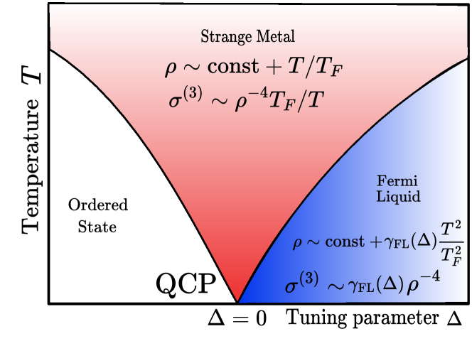
Figure 1: Figure schematically shows the temperature dependence of linear resistivity (in units of $\hbar/e^{2}$) and third order conductivity (in units of $e^{4}/\hbar k_{F}^{2}T_{F}^{2}$) in the vicinity of a QCP in strange metals. In the quantum critical regime (in red), where linear resistivity is linear in temperature, third order conductivity scales as $T_{F}/T$. In the Fermi liquid regime (in blue), where linear resistivity is quadratic in temperature, the third order conductivity is constant in the leading order in temperature. The dimensionless constant $\gamma_{\mathrm{FL}}(\Delta)$, where $\Delta$ is the boson gap, is of order $1$ in the ordinary FL state away from the QCP. On approaching the QCP, the coupling grows, resulting in $\gamma_{\mathrm{FL}}(\Delta)\sim c^{2}T_{F}^{2}/v_{F}^{2}\Delta^{2}$ dependence, where $c$ and $v_{F}$ are the critical boson and electron velocities, respectively. Qualitatively, in the quantum critical regime $\Delta^{2}\sim c^{2}T_{F}T/v_{F}^{2}$ resulting in the strange metal behavior.

Indeed, we find that the leading order non-linear response and the Joule heating response expressions can be expressed only through the quantities that appear in the linear conductivity of a corresponding model (Eq. (4) or Eq. (5)) and the parameters of the Fermi surface:

$${\sigma^{(3)}}^{a,bcd}(\nu_{b},\nu_{c},\nu_{d}) =\frac{\hbar A(T)}{e^{4}k_{F}^{4}v_{F}^{2}}\sigma(T,\nu_{d})\,\sigma^{2}(T,\nu_{bcd})\,\sigma(T,\nu_{cd})\,\Delta_{a,bcd}+(b,c,d\quad\mathrm{permutations}),$$ (6)

$${\sigma^{(3)}_{J}}^{a,bcd}(\nu_{b},\nu_{c},\nu_{d}) =\frac{\gamma_{J}A(T)}{2\pi e^{2}k_{F}^{3}v_{F}}\frac{\sigma(T,\nu_{d})\sigma^{2}(T,\nu_{bcd})\delta_{ab}\delta_{cd}}{i\nu a(T)+\Gamma_{0}(T)}+(b,c,d\quad\mathrm{permutations}).$$ (7)

Quantities $v_{F}$ and $k_{F}$ are Fermi velocity and Fermi wavenumber, $\sigma(T,\nu)$ is the linear conductivity defined by the model, $A(T)$ is a dimensionless function of temperature $T$ that describes the relative strength of the third order response, and $\gamma_{J}$ is a number of the order of unity that we will provide below. The tensor structure of non-linear response $\Delta_{a,bcd}$ can be obtained from

$$[\Delta_{x,bcd},\Delta_{y,bcd}]=[\,\mathrm{Re}\,(u_{b}u_{c}u_{d}),-\,\mathrm{Im}\,(u_{b}u_{c}u_{d})],\quad u=(1,i),$$ (8)

and we will discuss model-dependent renormalized mass $a(T)$ when we discuss Joule heating. Note that this form is only suitable for the models with a sharp momentum dependence of Green’s functions near Fermi surface, since $k_{F}$ and $v_{F}$ are undefined otherwise. To obtain the Fermi-liquid or strange metal values for the non-linear conductivity using in the Eqs. (7) and (6), one has to substitute $\sigma_{\mathrm{FL}}$ and $A_{\mathrm{FL}}$ or $\sigma_{\mathrm{nFL}}$ and $A_{\mathrm{nFL}}$ correspondingly. Let’s start from comparing the structure of the ordinary non-linear response. The corresponding expressions for $A_{\mathrm{FL}}$ and $A_{\mathrm{nFL}}$ in that regime are given by

$$A_{\mathrm{nFL}}(T) =\frac{2\pi^{2}e^{2}v_{F}^{2}k_{F}^{2}}{3}\frac{\alpha_{\rho}}{\gamma(T)T}\sim\frac{T_{F}}{T}.$$ (9)

$$A_{\mathrm{FL}} =3\hbar e^{2}k_{F}^{2}v_{F}^{2}\kappa_{\rho}=\gamma_{\mathrm{FL}}(\Delta)\sim\sim\mathrm{const},$$ (10)

since $\hbar v_{F}k_{F}\sim\varepsilon_{F}$ and we expect $\alpha_{\rho}\sim 1/e^{2}T_{F}$ according to [34]. The behavior of $\gamma_{\mathrm{FL}}(\Delta)$ depends on the proximity to the QCP. For ordinary Fermi Liquid away from QCP we expect $\gamma_{\mathrm{FL}}\sim 1$, while on the approach to QCP the coupling grows as $\gamma(\Delta)\sim c^{2}T_{F}^{2}/v_{F}^{2}\Delta^{2}$. Parameter $\Delta$ is a $T=0$ mass gap, $c$ is a critical boson velocity. At the scale of $\Delta^{2}\sim c^{2}T_{F}T/v^{2}$ the quantum critical regime starts and the strange metal response scalings are anticipated. Thus, as we argued above, the third order non-linear conductivity for strange metal has an enhanced relative strength in comparison to Fermi liquids. Moreover, as temperature decreases, we expect the third order conductivity to diverge as $T_{F}/T$ for strange metals, in contrast the third order conductivity in Fermi liquids is expected to be featureless. We schematically mark the linear resistivity and third order conductivity scaling in Fig. 1. Note, however, that in the vicinity of the QCP $A_{\mathrm{FL}}$ is still expected to be $T$-independent in the leading order, but is enhanced by a factor of $T_{F}^{2}/\Delta^{2}$, where $\Delta$ is a boson gap in the $v-g^{\prime}$ model, when away from the quantum critical point.

Now we compare the structure of the Joule heating terms between the strange metals and Fermi-liquids. We consider two phenomenological limits. In one limit, we consider an ”optical” regime, where the external frequency $\nu$ is so large that the energy relaxation rate $\Gamma_{0}$ can be neglected. Physically that corresponds to response on short time scales, at which energy doesn’t dissipate. In model of strange metal we obtained $\Gamma_{0}=0$ for boson dynamics included, thus it would be logical to compare it to the Fermi liquid response in the regime where $\Gamma_{0}$ can be neglected too. The dynamic dimensionless coefficients $a(T)$ that appear in Eq. (7) in the corresponding theories are given by

$$a_{\mathrm{FL}} =\frac{e^{2}k_{F}v_{F}}{2\pi\hbar}\rho_{\mathrm{FL},\nu},$$ (11)

$$a_{\mathrm{nFL}}(T) =\frac{e^{2}k_{F}v_{F}}{2\pi\hbar}\beta_{\rho}\ln\left(\frac{T_{\Gamma}}{T}\right).$$ (12)

Relevant expression for the Joule heating contribution in the optical limit is

$${\sigma^{(3)}_{\mathrm{nFL},J}}^{a,bcd}(\nu_{b},\nu_{c},\nu_{d}) =\frac{\gamma_{J}A_{\mathrm{nFL}}(T)}{e^{2}k_{F}^{3}v_{F}}\frac{\sigma_{\mathrm{nFL}}(T,\nu_{d})\sigma_{\mathrm{nFL}}^{2}(T,\nu_{bcd})\delta_{ab}\delta_{cd}}{i\nu a_{\mathrm{nFL}}(T)+\Gamma_{0}(T)}+(b,c,d\quad\mathrm{permutations}),$$ (13)

$${\sigma^{(3)}_{\mathrm{FL},J}}^{a,bcd}(\nu_{b},\nu_{c},\nu_{d}) =\frac{A_{\mathrm{FL}}(T)}{e^{2}k_{F}^{3}v_{F}}\frac{\sigma_{\mathrm{FL}}(T,\nu_{d})\sigma_{\mathrm{FL}}^{2}(T,\nu_{bcd})\delta_{ab}\delta_{cd}}{i\nu a_{\mathrm{FL}}(T)+\Gamma_{0}(T)}+(b,c,d\quad\mathrm{permutations}),$$ (14)

The dimensionless coefficient $\gamma_{J}=2+2\gamma(T)$ is the effect of non-linear corrections into the strange metal collision integral. If the collision integral was linear, we would expect $\gamma_{J}=1$. Note, however, that we neglected some details of frequency dependence of the linear conductivity when providing Eq. (13). The full analysis can be found in the main text. Again, since both of the Fermi liquid and strange metal responses have a similar structure, only the differences of $a(T)$ and $A(T)$ in different theories define the relative strength of the response. Since $A_{\mathrm{nFL}}$ in enhanced in comparison to $A_{\mathrm{FL}}$ at low temperatures, we expect stronger Joule heating effects in the optical limit for strange metals.

At low frequencies and temperatures, the energy relaxation rate values become important. In Fermi liquids is typically mediated by phonons with $\Gamma_{0}\sim T$ above the Bloch-Gruneisen temperature and $\sim T^{5}$ below it. Below we demonstrate that if the bosons in the non-Fermi liquid are kept in thermal equilibrium, they lead to a $\Gamma_{0}\sim T$ dependence at all temperatures. Thus, heating effects in nonlinear transport should be stronger in non-Fermi liquids at least in the whole range for Bloch-Gruneisen to Fermi temperature. However, since the energy relaxation of boson has not been currently explored, it is also possible that the actual energy relaxation rate in a non-Fermi liquid will be smaller at low T. Here we consider two extreme limits (bosons in thermal equilibrium always or energy conservation in the fermion+boson system) and leave the investigation of potential energy relaxation mechanisms for future work.

Finally, from the structure of the solution to the kinetic equation we have been able to conjecture the scaling with $T$ of all the higher order non-linear responses, and thus the response function in general. The strange-metal non-linear response current takes a form

$$|\mathbf{j}_{\mathrm{nFL},\mathrm{nl}}|\sim\frac{T^{2}\sigma(T)}{ev_{F}}F_{\mathrm{nFL}}\left(\frac{\sigma(T)|\mathbf{E}|}{ek_{F}T},\frac{\alpha_{\rho}T}{\rho_{0}}\right),$$ (15)

which has a universal scaling structure $|\mathbf{E}|/T$ for low temperatures $\alpha_{\rho}T\lesssim\rho_{0}$, while the non-linear response in Fermi-liquids remains featureless due to being suppressed by $T\sqrt{\hbar\sigma/e^{2}}/\varepsilon_{F}\ll 1$:

$$|\mathbf{j}_{\mathrm{FL},\mathrm{nl}}|\sim\frac{T^{2}\sigma(T)}{ev_{F}}F_{\mathrm{FL}}\left(\frac{\sigma(T)|\mathbf{E}|}{ek_{F}\sqrt{\Gamma\varepsilon_{F}}},\frac{T}{\varepsilon_{F}}\right).$$ (16)

where $\Gamma$ is a relaxation rate due to potential disorder defined as $\Gamma=\rho_{0}/4\pi e^{2}v_{F}k_{F}$. In the expressions functions $F_{\mathrm{nFL}}$ and $F_{\mathrm{FL}}$ do not depend on temperature explicitly. Note that the universal $|\mathbf{E}|/T$ scaling in strange metals is only applicable as far as $|\mathbf{E}|/T\lesssim 1$. Thus, decrease in temperature also requires an decrease in the amplitude of an external field to observe the sampling. Decreasing temperature $T$ while keeping $|\mathbf{E}|$ constant would only lead to a very different regime where $|\mathbf{E}|/T$ scaling might no longer hold.

A similar statement can be conjectured about the Joule heating-related non-linear response current density in the optical limit:

$$|\mathbf{j}_{J,\mathrm{nFL}}|\sim\frac{eT^{2}k_{F}}{\sqrt{\Gamma\nu\tilde{a}(T)}}F_{J,\mathrm{nFL}}\left(\frac{ev_{F}|\mathbf{E}|}{T\sqrt{\Gamma\nu\tilde{a}(T)}}\right),$$ (17)

while the Fermi-liquid result, again, remained featureless in terms of temperature dependence:

$$|\mathbf{j}_{J,\mathrm{FL}}|\sim ek_{F}a_{\mathrm{FL}}\nu\sqrt{\frac{\varepsilon_{F}}{\Gamma}}F_{J,\mathrm{FL}}\left(\frac{ev_{F}|\mathbf{E}|}{i\nu a_{\mathrm{FL}}\sqrt{\Gamma\varepsilon_{F}}}\right).$$ (18)

The expressions above are valid for a small $T$ limit. This shows that the strength of non-linear responses in strange metal is in general controlled by temperature. Thus, one would expect the material at low temperatures to become highly non-linear with a large number of higher order responses excited simultaneously. On this accord we conclude the showcase of results in the paper and proceed towards the calculation discussion in the following section of the paper.

II The model

To model a strange metal we use the so-called $v-g^{\prime}$ model [20, 21, 22, 24]. This model consists of $N$ flavors of fermionic fields $\psi_{i}(x)$ coupled to $N$ flavors of near-critical bosonic fields $\phi_{i}(x)$ through a spatial-dependent coupling $g_{ijl}^{\prime}(\mathbf{r})$. The bosonic mode in a strange metal can play the role of a near-critical collective fermion mode. The model The action for the model can be written as

$$S_{\mathrm{eq}}[\psi,\phi]=S_{0}[\psi,\phi]+S_{v}[\psi,\phi]+S_{g^{\prime}}[\psi,\phi],$$ (19)

where $S_{0}$ is a bare 1-particle action terms are

$$S_{0}[\psi,\phi]=\sum_{i=1}^{N}\int d^{3}x\;\psi_{i}^{\dagger}(x)\left[i\partial_{t}-\varepsilon(\hat{\mathbf{p}})-e\hat{\mathbf{p}}\cdot\mathbf{A}\right]\psi_{i}(x)\\ +\sum_{i=1}^{N}\int d^{3}x\;\frac{1}{2}\phi_{i}(x)\left[-\partial_{t}^{2}+c^{2}\nabla^{2}-m_{B}^{2}\right]\phi_{i}(x).$$ (20)

There $x$ is a shorthand notation for the time and space coordinates $(t,\mathbf{r})$. The $\epsilon(\hat{p})$ is an energy operator for the fermions, and $m_{B}$ is a bare mass of the bosonic mode, $c$ is a velocity of the bosonic mode. We couple the fermions to a gauge filed $A$ through a minimal coupling. In this paper we will restrict ourselves to the case of a spatially homogenious electric field, so $\mathbf{E}=\partial_{t}\mathbf{A}(t)$. The second term in Eq. (19) corresponds to potential disorder described by a chemical potential $v_{ij}(\mathbf{r})$:

$$S_{v}[\psi,\phi]=\frac{1}{\sqrt{N}}\sum_{i,j=1}^{N}\int d^{3}x\;v_{ij}(\mathbf{r})\psi_{i}^{\dagger}(x)\psi_{l}(x).$$ (21)

The third term in Eq. (19) is the spatial-dependent interaction

$$S_{g^{\prime}}[\psi,\phi]=\frac{1}{N}\sum_{i,j,l=1}^{N}\int d^{3}x\;c\,g^{\prime}_{ijl}\psi_{i}^{\dagger}(x)\psi_{j}(x)\phi_{l}(x).$$ (22)

The choice of the coupling constant $g^{\prime}$ to have an explicit prefactor of $c$ is merely a convenience that does not contradict [22] in any way. Since we are interested in computing the model non-linear response to the electric field by using the method of kinetic equations, we are going to apply the Keldysh approach to this system. Therefore, we define the Keldysh action as $S=S_{\mathrm{eq}}[\psi_{+},\phi_{+}]-S_{\mathrm{eq}}[\psi_{-},\phi_{-}]$, where the fields $\psi_{+}$ and $\phi_{+}$ are in the forward propagating part of the Keldysh contour, and $\psi_{-}$ and $\phi_{-}$ are in the backward propagating part. For our convenience, we introduce the Greek letter indices for the notation of the ”$+$” and ”$-$” fields:

$$\phi_{\lambda i}(x)=\begin{bmatrix}\phi_{+i}(x)\\ \phi_{-i}(x)\end{bmatrix},\quad\psi_{\alpha i}(x)=\begin{bmatrix}\psi_{+i}(x)\\ \psi_{-i}(x)\end{bmatrix}$$ (23)

With this notation in hand, we can write down our action as

$$S=\sum_{i=1}^{N}\int d^{3}x\,d^{3}x^{\prime}\;\psi_{\alpha i}^{\dagger}(x)G_{0\,\alpha\beta}^{-1}(x,x^{\prime})\psi_{\beta i}(x)\\ +\frac{1}{2}\sum_{i=1}^{N}\int d^{3}x\,d^{3}x^{\prime}\;\phi_{\rho i}(x)D_{0\,\rho\lambda}^{-1}(x,x^{\prime})\phi_{\lambda i}(x^{\prime})\\ +\frac{1}{\sqrt{N}}\sum_{i,j=1}^{N}\int d^{3}x\;v_{ij}(\mathbf{r})\psi_{\alpha i}^{\dagger}(x)\tilde{\delta}_{\alpha\beta}\psi_{\beta i}(x)\\ +\frac{1}{N}\sum_{i,j,l=1}^{N}\int d^{3}x\;cg^{\prime}_{ijl}(\mathbf{r})\tilde{\delta}_{\alpha\beta\lambda}\psi^{\dagger}_{\alpha i}(x)\psi_{\beta j}(x)\phi_{\lambda l}(x).$$ (24)

In the above equation, the new indexed objects $\tilde{\delta}_{\alpha\beta}$ and $\tilde{\delta}_{\alpha\beta\lambda}$ are responsible for the causality structure of the action. The $\tilde{\delta}_{\alpha\beta}$ coefficients are defined as

$$\tilde{\delta}_{\alpha\beta}=\begin{bmatrix}1&0\\ 0&-1\end{bmatrix},$$ (25)

while the $\tilde{\delta}_{\alpha\beta\lambda}$ are defined as

$$\tilde{\delta}_{+++}=-\tilde{\delta}_{---}=1$$ (26)

with all the other components being 0. Note that in the following calculations we will be performing a Keldysh rotation. We use the Kamenev convention [31], where bosons and fermions transform differently. Thus we reserve $\alpha$, $\beta$, $\mu$, and $\nu$ to correspond to the fermion causality indices, and $\lambda$ and $\rho$ for the boson causality indices.

The operators $G_{0\,\alpha\beta}^{-1}$ and $D_{0\,\rho\lambda}^{-1}$ are the inverses of bare Green’s functions defined in Eq. (20) with the corresponding causal structure induced by the Keldysh approach. Their form will be given after the Keldysh rotation is performed. From now on we will only be working with the action written in the notation of Eq. (24).

At last, we are going to assume that the potential disorder $v_{ij}(\mathbf{r})$ and the coupling $g^{\prime}_{ijl}(\mathbf{r})$ are random in the flavor and spatial coordinate. Therefore, averaging over the classical ensemble of the disorder results in

$$\left\langle v_{ij}(\mathbf{r})\right\rangle =\left\langle g^{\prime}_{ijl}(\mathbf{r})\right\rangle=0,$$ (27)

$$\left\langle v_{ij}^{*}(\mathbf{r})v_{ab}(\mathbf{r}^{\prime})\right\rangle =v^{2}\delta_{ia}\delta_{jb}\,\delta(\mathbf{r}-\mathbf{r}^{\prime}),$$ (28)

$$\left\langle g^{*\prime}_{ijl}(\mathbf{r})g^{*\prime}_{abc}(\mathbf{r}^{\prime})\right\rangle =g^{\prime 2}\delta_{ia}\delta_{jb}\delta_{lc}\,\delta(\mathbf{r}-\mathbf{r}^{\prime}),$$ (29)

where the averaging is done over the gaussian-distributed variables $v_{ij}$ and $g^{\prime}_{ijl}$:

$$\langle f\rangle=\int D[v,g^{\prime}]f(v,g^{\prime})e^{-\frac{v_{ij}^{2}(\mathbf{r})}{2v^{2}}}e^{-\frac{g^{\prime 2}_{ijl}(\mathbf{r})}{2g^{\prime 2}}}$$ (30)

In the next chapter we are going to perform the large-$N$ expansion for this model with the use of $\Sigma-G$ action in the Keldysh formalism.

III Saddle point equations

Following the usual procedure of $\Sigma-G$ method [20, 21, 22], we define the bilocal Green’s funtions fields

$$iG_{\alpha\beta}(x,x^{\prime})=\frac{1}{N}\sum_{i=1}^{N}\psi_{\alpha i}(x)\psi^{\dagger}_{\beta i}(x^{\prime}),$$ (31)

$$iD_{\rho\lambda}(x,x^{\prime})=\frac{1}{N}\sum_{i=1}^{N}\phi_{\rho i}(x)\phi_{\lambda i}(x^{\prime}).$$ (32)

In terms of these new fields $G$ and $D$, and their corresponding constraints Lagrange multipliers $\Sigma$ and $\Pi$ (self-energies), the effective action after integrating out the $\psi$ and $\phi$ fields is

$$\frac{S_{\mathrm{eff}}}{N}=-i\;\mathrm{Tr}\;\ln\left(G_{0}^{-1}-\Sigma\right)+\frac{i}{2}\;\mathrm{Tr}\;\ln\left(D_{0}^{-1}-\Pi\right)\\ +i\int d^{3}x\,d^{3}x^{\prime}\left(\frac{1}{2}\Pi_{\lambda\rho}(x^{\prime},x)D_{\rho\lambda}(x,x^{\prime})-\Sigma_{\alpha\beta}(x^{\prime}x)G_{\beta\alpha}(x,x^{\prime})\right)\\ +\frac{iv^{2}}{2}\int d^{3}x\,d^{3}x^{\prime}\;\delta(\mathbf{r}-\mathbf{r}^{\prime})\tilde{\delta}_{\alpha\beta}\tilde{\delta}_{\mu\nu}G_{\nu\alpha}(x^{\prime},x)G_{\beta\mu}(x,x^{\prime})\\ -\frac{c^{2}g^{\prime 2}}{2}\int d^{3}x\,d^{3}x^{\prime}\;\tilde{\delta}_{\alpha\beta\rho}\tilde{\delta}_{\mu\nu\lambda}G_{\nu\alpha}(x^{\prime},x)G_{\beta\mu}(x,x^{\prime})D_{\rho\lambda}(x,x^{\prime}).$$ (33)

This complicated expression consists of several parts. The traces in the first line of Eq. (33) comes from integrating out the fields $\psi$ and $\phi$. The terms with self-energies comes from the Lagrange multipliers. The term in the third line corresponds to the potential disorder, and finally, the last line corresponds to the randomized interaction.

Since the whole action is proportional to $N$, we apply a large-$N$ expansion that leads to the equations of motion for fields $G,D,\Sigma$, and $\Pi$ for the action that correspond to the saddle point of the action in Eq. (33).

Varying over the self-energies results in the Dyson equations

$$G_{\alpha\beta}(x,x^{\prime}) =\left[\left(G_{0}^{-1}-\Sigma\right)^{-1}\right]_{\alpha\beta}(x,x^{\prime}),$$ (34)

$$D_{\rho\lambda}(x,x^{\prime}) =\left[\left(D_{0}^{-1}-\Pi\right)^{-1}\right]_{\rho\lambda}(x,x^{\prime}).$$ (35)

Varying the action over $G$ results in

$$i\Sigma_{\alpha\beta}(x,x^{\prime})=i\Sigma_{v,\alpha\beta}(x,x^{\prime})+i\Sigma_{g^{\prime},\alpha\beta}(x,x^{\prime}),$$ (36)

The corresponding $v$ and $g^{\prime}$ components are

$$i\Sigma_{v,\alpha\beta}(x,x^{\prime}) =iv^{2}\delta(\mathbf{r}-\mathbf{r}^{\prime})\tilde{\delta}_{\alpha\mu}\tilde{\delta}_{\nu\beta}G_{\mu\nu}(x,x^{\prime})$$ (37)

$$i\Sigma_{g^{\prime},\alpha\beta}(x,x^{\prime}) =-\frac{c^{2}g^{\prime 2}}{2}\delta(\mathbf{r}-\mathbf{r}^{\prime})\tilde{\delta}_{\alpha\nu\rho}\tilde{\delta}_{\mu\beta\lambda}G_{\nu\mu}(x,x^{\prime})\left(D_{\rho\lambda}(x,x^{\prime})+D_{\lambda\rho}(x^{\prime},x)\right).$$ (38)

Varying over $D$ results in

$$i\Pi_{\lambda\rho}(x,x^{\prime})=c^{2}g^{\prime 2}\delta(\mathbf{r}-\mathbf{r}^{\prime})\tilde{\delta}_{\alpha\beta\rho}\tilde{\delta}_{\mu\nu\lambda}G_{\nu\alpha}(x,x^{\prime})G_{\beta\mu}(x^{\prime},x).$$ (39)

The Eqs (36) and (39) correspond to 1-loop corresponding expansions in the Keldysh theory. In the next section we will use these results to construct a kinetic equation that would describe $v-g^{\prime}$ model.

The equations obtained above have a proper form to be converted into a kinetic equation. However, before proceeding to the Keldysh kinetic equation, we need to complete the Keldysh rotation, where the distinction between fermoionic and bosonic casuality indices becomes important, since they transform differently in the convention employed in [31]. The Keldysh rotation for bosons is

$$\begin{bmatrix}\phi_{\mathrm{cl}}\\ \phi_{\mathrm{q}}\end{bmatrix}=\frac{1}{\sqrt{2}}\begin{bmatrix}1&1\\ 1&-1\end{bmatrix}\begin{bmatrix}\phi_{+}\\ \phi_{-}\end{bmatrix}.$$ (40)

We denote the transformation matrix used above as $\Lambda_{\rho\lambda}$. For the fermions the transformation is more complicated, since the conjugated fields transform differently from their counterparts:

$$\begin{bmatrix}\psi_{1}\\ \psi_{2}\end{bmatrix}=\frac{1}{\sqrt{2}}\begin{bmatrix}1&1\\ 1&-1\end{bmatrix}\begin{bmatrix}\psi_{+}\\ \psi_{-}\end{bmatrix},\quad\begin{bmatrix}\psi_{1}^{\dagger}\\ \psi_{2}^{\dagger}\end{bmatrix}=\frac{1}{\sqrt{2}}\begin{bmatrix}1&-1\\ 1&1\end{bmatrix}\begin{bmatrix}\psi_{+}^{\dagger}\\ \psi_{-}^{\dagger}\end{bmatrix}.$$ (41)

We denote the transformation matrix for the fields $\psi$ as $U_{\alpha\beta}$ and for $\psi^{\dagger}$ – as $V_{\alpha\beta}$. Then Green’s functions in the old basis are expressed through the Green’s functions in the new basis as

$$[D]_{\mathrm{old}}(x,x^{\prime})=\Lambda^{-1}[D]_{\mathrm{new}}(x,x^{\prime})(\Lambda^{-1})^{T},$$ (42)

where the RHS involves the Green’s function after the Keldysh rotation, and LHS involves the Green’s function before the Keldysh rotation. A similar expression for the fermions’ Green’s functions looks like

$$[G]_{\mathrm{old}}(x,x^{\prime})=U^{-1}[G]_{\mathrm{new}}(x,x^{\prime})(V^{-1})^{T}.$$ (43)

This rotation allows to explicitly eliminate one of the four components of the 2x2 matrices $[G_{\alpha\beta}]_{\mathrm{old}}$ and $[D_{\rho\lambda}]_{\mathrm{old}}$ as redundant in the theory. Thus we obtain

$$G_{\alpha\beta}=\begin{bmatrix}G_{R}&G_{K}\\ 0&G_{A}\end{bmatrix}$$ (44)

for fermions and

$$D_{\rho\lambda}=\begin{bmatrix}D_{K}&D_{R}\\ D_{A}&0\end{bmatrix}.$$ (45)

Green’s functions $G_{R}$ and $D_{R}$ are the retarded Green’s functions, and $G_{A}$ and $D_{A}$ are advanced Green’s functions of the corresponding fields. We parametrize the Keldysh Green’s functions $D_{K}$ and $G_{K}$ by introducing functions $F(x,x^{\prime})$ and $F_{B}(x,x^{\prime})$ such that

$$G_{K} =G_{R}\circ(1-2F)-(1-2F)\circ G_{A}$$ (46)

$$D_{K} =D_{R}\circ(1+2F_{B})-(1+2F_{B})\circ D_{A}.$$ (47)

The notation of $A\circ B$ stands for

$$A\circ B=\int d^{3}y\;A(x,y)B(y,x^{\prime})$$ (48)

and functions $F(x,x^{\prime})$ and $F_{B}(x,x^{\prime})$ play the role of a quantum analog of distribution functions that are determined within the Keldysh formalism.

IV Keldysh kinetic equation

Now we proceed to derive the kinetic equation that corresponds to the action that we obtained in the previous section. Since we have both fermionic and bosonic fields in the system, we need to write down the equations that govern the evolution of both $F(x,x^{\prime})$ and $F_{B}(x,x^{\prime})$. However, we will not utilize a classic approach that directly derives the equations of motion for the mentioned functions (for example, see Kamenev [31]). Instead we derive analogous equations for a set of functions $G^{<}(x,x^{\prime})$ and $D^{<}(x,x^{\prime})$ defined as

$$G^{<} =-G_{R}\circ F+F\circ G_{A},$$ (49)

$$D^{<} =D_{R}\circ F_{B}-F_{B}\circ D_{A}.$$ (50)

It is motivated by the similarity between our system and the system studied in [35, 24]: both systems have equilibrium self-energies independent from momentum. This allows to write a simpler set of kinetic equations that do not involve any momentum information, unlike the equations that govern the evolution of $F$ and $F_{B}$. Following [35], we obtain the equations of motion for those quantities:

$$\left[G_{0}^{-1};\;G^{<}\right] =\frac{1}{2}\left(\Sigma_{K}\circ G_{A}-G_{R}\circ\Sigma_{K}\right)+$$

$$+\frac{1}{2}\left(\Sigma_{A}\circ G_{A}+G_{R}\circ\Sigma_{R}-\Sigma_{R}\circ G_{A}-G_{R}\circ\Sigma_{A}\right)+\Sigma_{R}\circ G^{<}-G^{<}\circ\Sigma_{A}.$$ (51)

$$\left[D_{0}^{-1};\;D^{<}\right] =\frac{1}{2}\left(\Pi_{K}\circ D_{A}-D_{R}\circ\Pi_{K}\right)+$$

$$+\frac{1}{2}\left(\Pi_{A}\circ D_{A}+D_{R}\circ\Pi_{R}-\Pi_{R}\circ D_{A}-D_{R}\circ\Pi_{A}\right)+\Pi_{R}\circ D^{<}-D^{<}\circ\Pi_{A}.$$ (52)

Further simplification of the expressions in Eqs. (51) and (52) and their conversion into the Fourier space is possible with a simultaneous application of a few steps: Wigner transform, small perturbation expansion, and introduction of the spectral density function.

We are interested in studying the quasi-classical limit of the theory, and therefore, instead of studying functions $A(x,x^{\prime})$. We assume that all the 2-point functions in the theory are slow-varying with the change of $(x+x^{\prime})/2$ and fast-varying with the change of $(x-x^{\prime})/2$. Thus, as a first step, we study the evolution of the Wigner transformed 2-point functions defined as

$$A(x,p)=\int d^{3}\tilde{x}\;e^{-ip\tilde{x}}A\left(x+\frac{\tilde{x}}{2},x-\frac{\tilde{x}}{2}\right),$$ (53)

where $p$ is a shorthand notation for a pair $p=(\omega,\mathbf{k})$, and $p\tilde{x}=-\omega\tilde{t}+\mathbf{k}\mathbf{\tilde{r}}$.

Note that the Wigner transform has the following the properties:

$$(A\circ B)(x,p)\approx A(x,p)B(x,p)+\frac{i}{2}\left(\frac{\partial A}{\partial x}\frac{\partial B}{\partial p}-\frac{\partial A}{\partial p}\frac{\partial B}{\partial x}\right)$$ (54)

and

$$(A(x,x^{\prime})B(x,x^{\prime}))=\int\frac{d^{3}q}{(2\pi)^{3}}A(x,q)B(x,p-q).$$ (55)

Eq. (54) is the central approximation of the theory that limits the applicability of the theory to the large wavelength and small frequency perturbations, since it involves the infinite series truncation under assumption that the higher order terms in the series are small.

Applying Eqs. (54) and (55) reveals the core property of $v-g^{\prime}$: due to a spatial disorder all the self-energies do not depend on their corresponding momenta regardless of a concrete form of Green’s functions, which proves that this is not only true in equilibrium case [20, 21, 22], but also in the non-equilibrium case too.

The second step of the transformations involves the assumptions about the perturbation structure. We assume that all the perturbations around the equilibrium distribution are small, and we can describe the system by a small perturbation around that equilibrium:

$$F(x,\omega,\mathbf{k}) =\bar{F}(\omega)+\delta F(x,\omega,\mathbf{k}),$$ (56)

$$F_{B}(x,\Omega,\mathbf{q}) =\bar{F}_{B}(\Omega)+\delta F_{B}(x,\Omega,\mathbf{q}),$$ (57)

where $\delta F\ll\bar{F}$ and $\delta F_{B}\ll\bar{F}_{B}$. In this paper we adopt the notation where we denote the equilibrium quantities with a bar, and the perturbation away from the equilibrium with $\delta$.

To compute all the terms in the non-linear response one would have to expand all the self-energies and the Green’s functions in the order of $\delta F$ and $\delta F_{B}$. However, it will lead to infinite sequences of terms, thus we will employ a different strategy that will involve defining analogous quantities to $\delta F$ and $\delta F_{B}$ to make the number of terms in the resulting equation finite. We will eventually retrieve all the orders of expansion in perturbation $\delta F$ and $\delta F_{B}$ from Eqs. (51) and (52), but for now we start from the linear order analysis.

We provide the algebraic details of the described above calculation in Appendix A. We demonstrate that to the feature of decoupled momenta in $v$-$g^{\prime}$ theory, the equations are subject to great simplification after the Wigner transform and expansion. Below we only state the main results of the algebraic calculations for completeness.

We assume that the equilibrium solution is consistent with the previous works [20, 21, 22] and takes a form

$$\bar{G}_{R}(\omega,\mathbf{k}) =\frac{1}{\omega-v_{F}k-k_{F}(\hat{\mathbf{k}}\cdot\mathbf{A})-\bar{\Sigma}_{R}(\omega,T)},$$ (58)

$$\bar{D}_{R}(\Omega,\mathbf{q}) =\frac{1}{\Omega^{2}-c^{2}q^{2}-m^{2}+ic_{d}\Omega}.$$ (59)

In our model the fermions have a spherically symmetric dispersion relation with bare dispersion linearized at the level of the Fermi surface. The behavior of the $\bar{\Sigma}_{R}(\omega,T)$ is self-consistently determined through the Dyson equations in equilibrium and yields $\Sigma_{R}(\omega=0,T=0)=-i\Gamma$ at $T=0$. The constant $\Gamma$ is purely determined by the chemical potential disorder $\Gamma=v^{2}k_{F}/2v_{F}$ where $v$ is determined by Eq. (28). This contribution to the imaginary part of self-energy is dominant at low temperatures and low frequencies. The imaginary part in the boson propagator is also self-consistently determined with the value of the constant $c_{d}=g^{\prime 2}c^{2}k_{F}^{2}/8\pi v_{F}^{2}$ being fixed. The mass of the boson is a produced purely by thermal noise around the quantum critical point at $T=0$ and according to [20, 21, 22] scales with temperature as $m^{2}\approx\pi c_{d}T/\ln(T_{\Lambda}/T)$, where $T_{\Lambda}$ is a UV cutoff in the theory.

Substitution of Eq. (58) into Wigner-transformed and linearized Eq. (39) yields

$$\delta\Pi_{R}(x,\Omega)=\delta\Pi_{A}(x,\Omega)=0$$ (60)

at all the orders of perturbation of the excitation, which implies $\delta D_{R}=\delta D_{A}=0$. The linearization of the Dyson equations connects $\delta G_{R}$ and $\delta\Sigma_{R}$ through

$$\delta G_{R}=\bar{G}_{R}\circ\delta\Sigma_{R}\circ\bar{G}_{R}.$$ (61)

Substitution of Eq. (58) into a linearized Dyson equation in Eq.(61) produces a simple condition:

$$\int dk\;\delta G_{R}(\omega,\mathbf{k})=0,$$ (62)

which is, in fact, also true at all the orders of perturbation in orders of $\delta F$ and $\delta F_{B}$.

The last step towards deriving a simplified kinetic equations is to employ the observation made by previous works [35, 24] that employ Keldysh field theory. Since we are working with sharp Fermi surface at large $k_{F}$ and the self-energies don’t depend on the magnitude of corresponding momenta, the resulting response on the level of $F$ and $F_{B}$ should not contain strong dependence on magnitude of $k$ or $q$ [35]. We combine the developments of [20, 21, 22] and [35] to define $k$- and $q$- independent spectral functions as

$$f(x,\omega,\hat{k}) =-iv_{F}\int_{-\infty}^{+\infty}\frac{dk}{2\pi}G^{<}(x,\omega,\mathbf{k}),$$ (63)

$$f_{B}(x,\Omega,\hat{q}) =\frac{2\pi i}{\;\mathrm{arctg}\,\left(\frac{c\Omega}{m^{2}}\right)}\,\int_{0}^{+\infty}\frac{qdq}{2\pi}D^{<}(x,\Omega,\mathbf{q}).$$ (64)

Their main feature is that they are linear in $F$ and $F_{B}$ due to Eqs. (49) and (50), but have all the information about momentum magnitudes $k$ and $q$ dependence being erased by the integral. The momentum information is erased in a self-consistent manner, since $G^{<}\approx F\,\mathrm{Im}\,G_{R}$, which corresponds to the spectral density function. When integrated over momentum, it becomes a distribution in excitation energy summed over all momenta. The complicated prefactors in Eqs. (63) and (64) are selected purely for conventional reason that sets $\bar{f}=\bar{F}=(e^{\beta\omega}+1)^{-1}$ and $\bar{f}_{B}=\bar{F}_{B}=(e^{\beta\Omega}-1)^{-1}$ for Green’s functions $G_{R}$ and $D_{R}$ satisfying Eqs. (58) and (59). Note that such result for $\bar{F}$ and $\bar{F}_{B}$ is a usual Keldysh field theory equilibrium result, while $\bar{f}$ and $\bar{f}_{B}$ form comes from the convention on the prefactors. An interesting extra abservation is that the linearized expression for $\delta f$ does not need a small external frequency expansion to be simplified exactly and yields

$$\delta f =-iv_{F}\int_{-\infty}^{+\infty}\frac{dk}{2\pi}\delta F\left(\bar{G}_{A}-\bar{G}_{R}\right),$$ (65)

This is, however, not true for $\delta f_{B}$, which involves an infinite tower of terms linear in $\delta f_{B}$ and it’s time derivatives of all orders. This is one of the infinite towers this method allows to evade during the calculation.

With all the features of the model discussed above, we execute the Wigner transform, expansion in perturbation, and finally integrate that version of Eqs. (51) and (52) over $k$ and $q$ correspondingly to obtain the system of closed equations for $\delta f$ and $\delta f_{B}$ at all the orders of expansion for the perturbations (see Appendix A for fairly involved algebraic details). We discuss the structure of the kinetic equation and its solution for the remainder of the paper.

Before we proceed, it is important to consider the limitations in our approach. The equations for $\delta f$ and $\delta f_{B}$ to be derived from the Eqs. (51) and (52) and the derivation involves Eq. (54), which for 2-point functions $A$ and $B$ holds only when $|\partial_{t}A\,\partial_{\omega}B|\ll|AB|$ and $|\partial_{\omega}A\,\partial_{t}B|\ll|AB|$. This automatically puts a set of constraints on the time derivative of $\delta f$ and $\delta f_{B}$ which can be written as

$$|\partial_{\omega}\,\mathrm{Re}\,\bar{\Sigma}_{R}\,\partial_{t}\delta f| \ll|\,\mathrm{Im}\,\bar{\Sigma}_{R}\,\delta f|$$ (66)

$$|\partial_{\omega}\bar{f}\partial_{t}\,\mathrm{Re}\,\delta\Sigma_{R}| \ll|(2\bar{f}-1)\,\mathrm{Im}\,\delta\bar{\Sigma}_{R}|$$ (67)

$$|C(\Omega)\partial_{t}\delta\Pi_{K}| \ll|\delta\Pi_{K}|$$ (68)

The first two conditions arise from the Wigner transformation of the terms $\Sigma_{R}\circ G^{<}$ and $G^{<}\circ\Sigma_{A}$ in Eq. (51). The third condition arises from the terms $\Pi_{K}\circ D_{A}$ and $D_{R}\circ\Pi_{k}$ in Eq. (52). These conditions simplify to a simple single condition

$$\nu\ll T$$ (69)

with the expressions for the involved quantities, which can be found in Appendix A. Note that this condition does not fulfill all the inequalities above for all values of $\omega$ and $\Omega$, however it works for all values besides $\Omega\ll T$ and $\omega\ll T$. However, since the range of frequencies where our theory breaks is small, the impact on the behavior is negligible.

IV.1 Boson in thermal equilibrium

At first, let’s consider the situation when the bosonic field is in a thermal state for simplicity. This can occur when the boson experiences a strong drag due to interaction with other parts of the system. If that interaction induces a drag much stronger then the interaction with the fermions, the boson relaxation time will be negligibly small and we can treat it as if it is in a thermal equilibrium. We will use this limit to phenomenologically understand the heating process in the material due to current circulation. To obtain the kinetic equation that governs the evolution of $\delta f$, we apply all the previously described steps to Eq. (51): the Wigner transform, expansion, and the algebraic simplification from $\delta G^{<}$ to $\delta f$ that captures all the orders in $\delta f$. The algebraic details of this calculation can be found in Appendix A. We thermalize bosonic degrees of freedom by fixing $\delta f_{B}=0$ and we obtain the kinetic equation of the form

$$A[\partial_{t}\,\delta f]-(\mathbf{v}_{F}\cdot\mathbf{E})\partial_{\omega}(\bar{f}+\delta f)=I_{\Gamma}[\delta f]+I_{g^{\prime}}[\delta f]+I_{\mathrm{nl}}[\delta f].$$ (70)

Even from the first glance the similarity between the form of Eq. (70) resembles the structure that we would expect in the ordinary Fermi-liquid theory, as in Eq. (1). However, it is instructive to discuss every term in it to see what novelty the model of strange metal in consideration brings in the contrast to ordinary Fermi-liquids.

The first term in the RHS of Eq. (70) is a renormalized dynamic term that only depends on $\partial_{t}\delta f$. The term itself involves a rather complicated linear functional $A$ that has a form

$$A[\partial_{t}\,\delta f]=a(\omega,T)\partial_{t}\,\delta f(\hat{k},\omega)+\frac{g^{\prime 2}k_{F}}{v_{F}}\partial_{\omega}\bar{f}\int\frac{d\Omega}{2\pi}B^{\prime}(\Omega)\int\frac{d\hat{\mathbf{k}}}{2\pi}\partial_{t}\,\delta f(\omega+\Omega,\hat{\mathbf{k}}).$$ (71)

Variable $\hat{\mathbf{k}}$ is the direction of momentum $\mathbf{k}$ that has been preserved in the theory. The function $a(\omega,T)$ is defined as $a=1-\partial_{\omega}\,\mathrm{Re}\,\bar{\Sigma}_{R}$ and the details of its structure are determined by the structure of the boson thermal mass $m^{2}(T)$. At a critical doping point

$$m^{2}(T)\approx\frac{\pi c_{d}T}{\ln(\frac{T_{\Lambda}}{T})},$$ (72)

which leads to $a(\omega,T)$ having a rather complicated structure at $T\neq 0$:

$$a(\omega)=1+\frac{g^{\prime 2}k_{F}}{8\pi^{2}v_{F}}\left[\ln\left(\frac{c^{2}\Lambda_{q}^{2}}{2\pi c_{d}T}\right)-\,\mathrm{Re}\,\psi^{(0)}\left(\frac{1}{2}-\frac{i\omega}{2\pi T}\right)\right],$$ (73)

where $\psi^{(0)}$ is a polygamma function of the $0$’th order. Relevant details to the derivation of this expression are shown in Appendix B. It is worth to note for the following sections that at $T=0$ the expression for $a(\omega,T=0)$ takes particularly simple form

$$a(\omega,T=0)=1+\frac{g^{\prime 2}k_{F}}{8\pi^{2}v_{F}}\ln\left|\frac{T_{\Lambda}}{\omega}\right|,$$ (74)

which is, interestingly, non-analytic at $\omega=0$. Temperature $T_{\Lambda}=ec^{2}\Lambda_{q}^{2}/c_{d}$ ($e$ being an Euler constant) is completely determined by the momentum UV-cutoff of the bosons $\Lambda_{q}$ that is necessary for the consistency of the theory [20, 22]. Thus this temperature to be expected to be much larger than any other parameter in the theory, in particular $T\ll T_{\Gamma}$. Function $B^{\prime}(\Omega)$ involved in Eq. (71) is described by

$$B^{\prime}(\Omega)=-c^{2}\int\frac{d^{2}q}{(2\pi)^{2}}\,\mathrm{Re}\,\bar{D}_{R}(\Omega,\mathbf{q})=\frac{1}{8\pi}\ln\left(\frac{c^{4}\Lambda_{q}^{4}}{m^{4}+c_{d}^{2}\Omega^{2}}\right).$$ (75)

The dynamic term has two main features that are distinctively different from Fermi-liquids. First feature is that in Fermi-liquids one would typically expect no strong dependence of $a(\omega,T)$ on $\omega$ or $T$, however in our case it is not true neither for $T>0$ or $T=0$ expression. Moreover, in the case of considered model the full dependence involves a complicated integral that mixes the dynamics in $\omega$ and in general needs to be diagonalized. The second feature is that the dependence in $\omega$ of the dynamic term is singular for $T=0$ and $\omega=0$ due to the logarithmic dependence of $a(\omega,T)$ as in Eq. (74), unlike in Fermi liquids. Note that this is not a sign of an inconsistency of the theory, since for $T>0$ the dependence is completely analytic, as in Eq. (73) (see Appendix B for more details).

Away from the critical doping the boson mass $m^{2}(T)\approx\Delta^{2}$ becomes temperature-independent, which leads to a $T$- and $\omega$-independent value of $a(\omega,T)$

$$a_{\mathrm{FL}}(\omega,T)=1+\frac{g^{\prime 2}k_{F}}{8\pi^{2}v_{F}}\ln\left(\frac{c^{2}\Lambda_{q}^{2}}{e\Delta^{2}}\right)\approx\mathrm{const},$$ (76)

which is fully consistent with our expectation for the Fermi-liquid in Sec. I. Additionally, away from the critical point the $c_{d}^{2}\Omega^{2}$ term in Eq. (75) can be neglected. Thus the integral term in Eq. (71) is proportional to the change of the particle number $\int d\omega d\hat{\mathbf{k}}\,\delta f(\omega,\hat{\mathbf{k}})$. Thus, since the particle number is expected to remain unchanged, the integral has to disappear. In the regime of a gapped boson $m^{2}\approx\Delta^{2}$, the dynamic term reduces to a constat factor $a$ in front of $\partial_{t}\delta f$, as expected in Sec. I.

We proceed to consider the collision integral terms $I_{\Gamma}$, $I_{g^{\prime}}$, and $I_{\mathrm{nl}}$. In this calculation we deliberately separated the terms in the collision integral into three categories, where every piece we diligently compute in Appendix A.

The term $I_{\Gamma}$ comes solely from the chemical potential disorder scattering. It has a simple form and its scattering rate $\Gamma$ does not explicitly depend on temperature or energy of the excitation, since $\Gamma=i\Sigma_{R}(\omega=0,T=0)$:

$$I_{\Gamma}[\delta f]=-2\Gamma\left(\delta f(\omega,\hat{\mathbf{k}})-\int\frac{d\hat{\mathbf{k}}^{\prime}}{2\pi}\delta f(\omega,\hat{\mathbf{k}}^{\prime})\right).$$ (77)

In addition, this term has no non-linear corrections in $\delta f$ and is computed exactly.

Terms $I_{g^{\prime}}$ and $I_{\mathrm{nl}}$ come from the interaction between the fermions and bosons. We split the interaction terms in such a way that $I_{g^{\prime}}$ only contains linear in $\delta f$ terms, while $I_{\mathrm{nl}}$ contains all quadratic in $\delta f$ terms. Note that there are no higher order corrections in powers of $\delta f$ in this formalism and the equation for $\delta f$ becomes exact. The structure of $I_{g^{\prime}}$ is rather complicated structure and involves two terms:

$$I_{g^{\prime}}[\delta f] =-2g(\omega,T)\,\delta f(\omega,\hat{\mathbf{k}})+\frac{g^{\prime 2}k_{F}}{v_{F}}\int\frac{d\Omega}{2\pi}B(\Omega)\left(2\bar{f}_{B}(\Omega)-2\bar{f}(\omega)+2\right)\int\frac{d\hat{\mathbf{k}}}{2\pi}\delta f(\omega+\Omega,\hat{\mathbf{k}}).$$ (78)

One of the terms contains a function $g(\omega,T)=\,\mathrm{Im}\,\bar{\Sigma}_{R}$, which, same as $a(\omega,T)$, is determined by the structure of $m^{2}(T)$, has a rather complicated $T$-dependence at the critical value of doping ($m^{2}(T)$ is given by Eq. (72)):

$$g(\omega,T)=\frac{g^{\prime 2}k_{F}}{8\pi v_{F}}T\left[\ln\left(\frac{2\pi c_{d}T}{m^{2}}\right)-2\,\mathrm{Re}\,\ln\Gamma\left(\frac{1}{2}-\frac{i\omega}{2\pi T}\right)\right].$$ (79)

Details for this calculation can be found in Appendix B. At $T=0$ it takes a particularly simple form:

$$g(\omega,T=0)=\frac{g^{\prime 2}k_{F}}{8\pi v_{F}}|\omega|.$$ (80)

Also note that the structure of $g(\omega,T)$ at $\omega=0$ is non-analytic when $T=0$, but is analytic when $T>0$, same as $a(\omega,T)$. This is another feature that is explicitly distinct from ordinary Fermi liquids where one would expect $g\sim(\pi^{2}T^{2}+\omega^{2})/\varepsilon_{F}$. However, the case of $m^{2}\approx\Delta^{2}$ yields

$$g_{\mathrm{FL}}(\omega,T)=\frac{g^{\prime 2}k_{F}c_{d}}{16\pi^{2}v_{F}\Delta^{2}}\left(\pi^{2}T^{2}+\omega^{2}\right),$$ (81)

which is exactly of the expected form. Additionally, at small enough $T$ one can expand the function $B(\Omega)$ in the powers of $\Omega\sim T$ in Eq. (78). This would lead to the temperature scaling of the integral term to be shifted away from $\sim T$ at the critical doping to $\sim T^{2}$, which we expect in the ordinary Fermi liquid.

In the following section we will show below that those non-analyticities of $g(\omega,T=0)$ and $a(\omega,T=0)$ at the critical doping, which are connected to $\omega/T$ dependence, are crucially important for the structure of higher order responses. Another function that is involved in the integral term of Eq. (78) is $B(\Omega)$, which is given by

$$B(\Omega)=-c^{2}\int\frac{d^{2}q}{(2\pi)^{2}}\bar{D}_{R}(\Omega,\mathbf{q})=\frac{1}{4\pi}\;\mathrm{arctg}\,\left(\frac{c_{d}\Omega}{m^{2}}\right).$$ (82)

The full structure of the term $I_{\mathrm{nl}}$ that contains all the non-linear in $\delta f$ corrections is shown in Appendix A. Its structure is rather complicated and involves quadratic expressions in $\delta f$ and derivatives of $\delta f$. However, we will only be interested in computing only third order non-linear response in the leading order in temperature dependence. The only relevant for this task term is rather simple and can be written as

$$I_{\mathrm{nl}}[\delta f]=-\frac{g^{\prime 2}k_{F}}{v_{F}}\int\frac{d\Omega}{2\pi}\int\frac{d\hat{\mathbf{k}}^{\prime}}{2\pi}B(\Omega)\left[\delta f(\omega+\Omega,\hat{\mathbf{k}}^{\prime})\delta f(\omega,\hat{\mathbf{k}})\right].$$ (83)

If one is interested in computing only the leading order of non-linear response, it is enough to use the expression for $I_{\mathrm{nl}}$ provided above. However, when we perform a structural analysis of the higher order responses, all the terms have to be considered. Note that a complete expression for all non-linear terms also involves terms proportional to $\partial_{t}\delta f$. Technically, those terms have to be regarded as the terms that belong to $A$ and they will make functional $A$ to be non-linear. However, in perturbation theory those terms will always play a role of lower order in electric field sources that are sub-leading to the term in Eq. (83).

As we expected, kinetic equation Eq. (210) is, in fact, a closed equation for $\delta f(\hat{k},\omega,t)$. We will explore the solution of this equation by the means of perturbation theory in electric field in the following sections. Now we proceed to modify the theory to include the boson dynamics.

IV.2 Full self-consistent boson dynamics

Now we proceed to include all the corrections that come into the kinetic equation when the boson is not thermalized and full dynamics of $\delta f_{B}$ has to be considered. To achieve this, we perform an analogous calculation to the one that was described above and led to Eq. (70). However, this time we set $\delta f_{B}\neq 0$ and include all the perturbative corrections in $\delta f_{B}$ ( algebra details in Appendix A). The calculation leads to an equation of the form

$$A[\partial_{t}\,\delta f]-(\mathbf{v}_{F}\cdot{\mathbf{E}})\partial_{\omega}(\bar{f}+\delta f)=I_{\Gamma}[\delta f]+I_{g^{\prime}}^{\prime}[\delta f,\delta f_{B}]+I_{\mathrm{nl}}^{\prime}[\delta f,\delta f_{B}].$$ (84)

It is useful to compare to the kinetic equation in Eq. (70). The close inspection shows that the dynamic term $A[\partial_{t}\delta f]$ and the disorder collision integral $I_{\Gamma}$ remained unchanged and are still described by Eqs. (71) and (77). The terms that did change are the linearized interaction-driven collision integral $I^{\prime}_{g^{\prime}}$, and the non-linear in $\delta f$ and $\delta f_{B}$ corrections. The new linearized collision integral now depends on both $\delta f$ and $\delta f_{B}$ and can be written as

$$I^{\prime}_{g^{\prime}}[\delta f,\delta f_{B}]=I_{g^{\prime}}[\delta f]+I_{c_{d}}[\delta f_{B}],$$ (85)

where the part $I_{g^{\prime}}$ that only depends on $\delta f$ is the same as in the case of thermalized boson and therefore described by Eq. (78). The new term that depends on $\delta f_{B}$ is

$$I_{c_{d}}[\delta f_{B}]=\frac{g^{\prime 2}k_{F}}{v_{F}}\int\frac{d\Omega}{2\pi}\int\frac{d\hat{q}}{2\pi}B(\Omega)(\bar{f}(\omega+\Omega)+\bar{f}(\omega-\Omega)-2\bar{f}(\omega))\,\delta f_{B}(\Omega,\hat{q}).$$ (86)

The non-linear corrections with the appearance of $\delta f_{B}\neq 0$ take a much more cumbersome form. The full structure is shown in Appendix A. However, the only leading order terms that appear in the 3rd order of the perturbation theory still have a rather simple form

$$I_{\mathrm{nl}}^{\prime}[\delta f,\delta f_{B}]=-\frac{g^{\prime 2}k_{F}}{v_{F}}\int\frac{d\Omega}{2\pi}\int\frac{d\hat{\mathbf{q}}}{2\pi}\int\frac{d\hat{\mathbf{k}}^{\prime}}{2\pi}B(\Omega)\left[2\,\delta f_{B}(\Omega,\hat{\mathbf{q}})\,\delta f(\omega,\hat{\mathbf{k}})+\delta f(\omega+\Omega,\hat{\mathbf{k}}^{\prime})\,\delta f(\omega,\hat{\mathbf{k}})\right].$$ (87)

Introduction of boson dynamics brings additional terms into the fermion kinetic equation in Eq. (84). These new terms depend on $\delta f_{B}$ and therefore we require an additional equation that governs the evolution of $\delta f_{B}$. We construct this equation by performing an already mentioned above simplification procedure on Eq. (52) (see Appendix A) in a similar manner as we did to derive the kinetic equations for fermions. The result of our calculation manifests itself in a form of

$$\partial_{t}\,\delta f_{B}+c_{d}\,\delta f_{B}=I_{B}[\delta f]+I_{B,\mathrm{nl}}[\delta f].$$ (88)

As a reminder, $c_{d}=g^{\prime 2}c^{2}k_{F}^{2}/8\pi v_{F}^{2}$, which is determined self-consistently from the analysis of the theory performed in a thermal equilibrium. Note, however, the analysis relies on the assumption that the system has no other fields besides the fermions and the collective mode described by the bosonic field. Introduction of other fields could lead to presences of additional thermal baths and therefore an additional drag, which will make the value of $c_{d}$ larger. The terms $I_{B}$ and $I_{B,\mathrm{nl}}$ are linearized and quadratic in $\delta f$ collision integral terms in the bosonic kinetic equation correspondingly. The linearized part of collision integral $I_{B}$ is given by

$$I_{B}[\delta f]=\frac{g^{\prime}c^{2}k_{F}^{2}}{2v_{F}^{2}}\int\frac{d\omega}{2\pi}\int\frac{d\hat{k}}{2\pi}\frac{1}{\Omega}\left(1-f(\omega-\Omega)-f(\omega+\Omega)\right)\times\left(\delta f-C(\Omega)\partial_{t}\delta f\right).$$ (89)

The function $C(\Omega)$ is

$$C(\Omega)=\frac{c_{d}^{2}\Omega}{2(m^{4}+c_{d}^{2}\Omega^{2})\;\mathrm{arctg}\,\left(\frac{c_{d}\Omega}{m^{2}}\right)}.$$ (90)

The quadratic in $\delta f$ correction to the collision integral $I_{B,\mathrm{nl}}$ leading term in the 3rd order becomes

$$I_{B,\mathrm{nl}}[\delta f]=\frac{c^{2}g^{\prime 2}k_{F}^{2}}{2v_{F}^{2}}\int\frac{d\omega}{2\pi}\int\frac{d\hat{\mathbf{k}}}{2\pi}\frac{d\hat{\mathbf{k}}^{\prime}}{2\pi}\,\frac{1}{\Omega}\left[\delta f(\omega-\Omega,\hat{\mathbf{k}})\delta f(\omega,\hat{\mathbf{k}}^{\prime})\right],$$ (91)

and there are no more higher order corrections in $\delta f$ or $\delta f_{B}$ to the boson kinetic equation in Eq. (88). Instead, there is a truncated tower of quadratic in $\delta f$ terms that involve derivatives over $\omega$ and $t$ of the quadratic expressions in $\delta f$. Those, however, are sub-leading due to $\nu<T$ and thus can be dropped, as all the non-linear corrections will only play a role of the extra source terms.

The collision integral terms $I_{B}$ and $I_{B,\mathrm{nl}}$ only depend on $\delta f$ and not $\delta f_{B}$, because all the scattering of bosons on each other is already self-consistently included into constant $c_{d}$. Thus, these terms should rather be interpreted as the coupling terms between the bosonic excitations $\delta f_{B}$ and fermionic excitations $\delta f$, even though these coupling terms originate from the term in Eq. (52) usually associated with the collision integral. Comparing the kinetic equations for bosons in Eq. (88) and fermions in Eq. (84) reveals that excitations $\delta f$ and $\delta f_{B}$ are coupled to each other through the collision integral terms in both of the equations. Now we are in a possession of the system of equations for $\delta f$ and $\delta f_{B}$, and the system of equations is closed for those unknown function. We can proceed to construct the perturbative solution to the system of equations in the following sections.

V Structure of the equations

Before we begin the construction of the perturbation theory in the powers of electric field, we need to analyze the structure of the equations that govern the evolution of $\delta f$ and $\delta f_{B}$. In this section we will explore the structure of the leading order terms in Eqs. (84) and (88), which means we will for now completely ignore the presence of $I_{\mathrm{nl}}$ and $I_{B,\mathrm{nl}}$. This simplification will not impact the dynamics of the response, since in the perturbation theory all the non-linear corrections play the role of the additional sources in addition to the source generated by electric field $\mathbf{E}$. We will reinstate the sources coming from non-linear corrections in the process of computing the non-linear responses in the next section.

We begin the analysis by implementing the angular harmonics expansion for $\delta f$ and $\delta f_{B}$:

$$\delta f(\omega,\hat{k}) =\sum_{m=-\infty}^{+\infty}\delta f_{m}(\omega)e^{im\theta_{k}},$$ (92)

$$\delta f_{B}(\Omega,\hat{q}) =\sum_{m=-\infty}^{\infty}\delta f_{Bm}(\Omega)e^{im\theta_{q}}.$$ (93)

The angles $\theta_{k}$ and $\theta_{q}$ are the angles that describe direction of unit vectors $\hat{\mathbf{k}}$ and $\hat{\mathbf{q}}$ correspondingly. This simplifies our analysis due to assumed spherical symmetry of the system. Implicitly we assume the dependence of $\delta f$ and $\delta f_{B}$ on $T$. From now on we will be using a lower index to signal the angular harmonic expansion or relation to a particular harmonic. The linearized equations that we are interested in analyzing have a form

$$A[\partial_{t}\delta f]+ev_{F}\,(\mathbf{E}\cdot\hat{\mathbf{k}})\,\partial_{\omega}(\bar{f}+\delta f)=(I_{\Gamma}+I_{g^{\prime}})[\delta f]+I_{c_{d}}[\delta f_{B}]$$ (94)

for fermions and

$$\partial_{t}\delta f_{B}+c_{d}\delta f_{B}=I_{B}[\delta f].$$ (95)

for bosons. As we mentioned above, these equations differ from the Eqs. (84) and (88) by the absence of non-linear terms $I_{\mathrm{nl}}$ and $I_{B,\mathrm{nl}}$. The fermionic collision integrals $I_{\Gamma}$ (scattering on potential disorder), $I_{g^{\prime}}$ (interaction with boson background), and $I_{c_{d}}$ (boson excitations) are described in Eqs. (77), (78), and (86) correspondingly. The bosonic collision integral that comes from the fermionic perturbations can be found in Eq. (89). We convert the kinetic equations into angular harmonics by integrating those over $\theta_{k}$ and $\theta_{q}$ with an appropriate exponent value. First we start from the harmonics $m\neq 0$ for simplicity. The integral terms in the linear functional $A$ and the collision integrals only depend on $\int d\hat{\mathbf{k}}\delta f$ or $\int d\hat{\mathbf{k}}\delta f_{B}$, which are proportional to $\delta f_{0}$ and $\delta f_{B0}$ correspondingly and have no directional dependence themselves. Thus those will have no effects for harmonics with $m\neq 0$ and the terms simplify to

$$a(\omega,T)\,\partial_{t}\delta f_{m}(\omega)+2\left(\Gamma+g(\omega,T)\right)\delta f_{m}(\omega)+\\ +\frac{ev_{F}}{2}\,\partial_{\omega}(\mathcal{E}^{*}\delta f_{m-1}(\omega)+\mathcal{E}\delta f_{m+1}(\omega))=-\frac{ev_{F}}{2}\,\partial_{\omega}\bar{f}(\omega)(\mathcal{E}^{*}\delta_{1,m}+\mathcal{E}^{*}\delta_{-1,m}).$$ (96)

In the equation above the first term corresponds to the $A[\partial_{t}\delta f]$ term, the second term corresponds to the remains of collision integrals $I_{\Gamma}$,$I_{g^{\prime}}$, and $I_{c_{d}}$, the last two terms correspond to the term with electric field $\mathbf{E}$. We introduced a shorthand notation for $\mathcal{E}=E_{x}+iE_{y}$ with $E_{x}$ and $E_{y}$ being the components of $\mathbf{E}$. The $\mathcal{E}^{*}$ is the complex conjugate of $\mathcal{E}$. A complete expression for the fermion evolution would also involve the extra source in the RHS of Eq. (96) generated by $I^{\prime}_{\mathrm{nl}}$ that has a form

$$I_{\mathrm{nl}}^{\prime}=-\frac{g^{\prime 2}k_{F}}{v_{F}}\int\frac{d\Omega}{2\pi}B(\Omega)\left[2\,\delta f_{B0}(\Omega)+\delta f_{0}(\omega+\Omega)\right]\delta f_{m}(\omega).$$ (97)

The expression for the case of thermalized boson can be obtained by setting $\delta f_{B0}=0$.

Analogous transformation for $m\neq 0$ for boson kinetic equation in Eq. (95) has a simple form:

$$\partial_{t}\delta f_{Bm}+c_{d}\delta f_{Bm}=0,\quad m\neq 0.$$ (98)

Notice that $\delta f_{Bm}$ for $m\neq 0$ is completely decopled from $\mathbf{E}$ and all the other harmonics of both fermionic and bosonic fields. Therefore those will stay relaxed at all the levels of perturbation theory and

$$\delta f_{Bm}=0,\quad m\neq 0.$$ (99)

Thus all the effects of the boson dynamics are described by the evolution of $\delta f_{B0}$.

We proceed to analyze the kinetic equations projected on the $0$’th harmonic $\delta f_{0}$ and $\delta f_{B0}$. Since the scattering on the chemical potential disorder always conserves every, $I_{\Gamma}[\delta f_{0}]=0$ and equation for $\delta f_{0}$ becomes

$$A[\partial_{t}\delta f_{0}]+ev_{F}\,\partial_{\omega}(\mathcal{E}\delta f_{1}+\mathcal{E}^{*}\delta f_{-1})=I_{g^{\prime}}[\delta f_{0}]+I_{c_{d}}[\delta f_{B0}].$$ (100)

Note that the fermion density harmonic $\delta f_{0}$ only couples to harmonics $\delta f_{\pm 1}$ and the boson density harmonic $\delta f_{B0}$. Therefore, the dynamics of the boson only impacts the dynamics of the density harmonic of the fermion. Same as in the case of $m\neq 0$, the corresponding non-linear corrections can be restored, however, there will be no non-linear corrections into the density harmonic below the 4’th order response.

For the density harmonic of the boson $\delta f_{B0}$ we acquire a following equation:

$$\partial_{t}\delta f_{B0}+c_{d}\delta f_{B0}=I_{B}[\delta f_{0}].$$ (101)

The boson perturbations are only coupled to the perturbations of the fermion density harmonic $\delta f_{0}$. The coupling of only density harmonics in our theory is a result of all the interactions between the boson and the fermion governed by a spatially random potential, which prohibits the momentum transfer. Due to the structure of non-linear correction terms, there will be no contributions below the 4’th order response.

Before we proceed to construct the perturbation theory series in $\mathbf{E}$ (or, equivalently, in $\mathcal{E}$), we need to understand the structure of the equations for the density harmonics $\delta f_{0}$ and $\delta f_{B0}$ better. The $\omega$-dependence of $A[\partial_{t}\delta f_{0}]$, $I_{g^{\prime}}[\delta f_{0}]$, and $I_{c_{d}}[\delta f_{B0}]$ along with $\Omega$-dependence of $I_{B}[\delta f_{0}]$ is of a particular interest, since it will turn out that the collective dynamics of the density harmonics is crucial for understanding the higher order responses. Below we describe our short studies of the structure of frequency dependence and show that the theory contains a few surprising properties that will allow us to construct a simplified but realistic model of the higher order optical responses.

At first we analyze the structure of $A$ linear functional and show that it’s action in the low temperature limit reduces to a multiplication by a constant in the case of anti-symmetric in $\omega$ argument $\delta f_{0}$. In the following sections we will show that this is exactly the case for $\delta f_{0}$ in the perturbation theory. The expression for $A[\delta f_{0}]$ dictates that

$$A[\partial_{t}\,\delta f_{0}]=a(\omega,T)\partial_{t}\,\delta f_{0}(\omega)+\frac{g^{\prime 2}k_{F}}{v_{F}}\partial_{\omega}\bar{f}\int\frac{d\Omega}{2\pi}B^{\prime}(\Omega)\partial_{t}\,\delta f_{0}(\omega+\Omega).$$ (102)

The expression for $B^{\prime}(\Omega)$ is

$$B^{\prime}(\Omega)=\frac{1}{8\pi}\ln\left(\frac{c^{4}\Lambda_{q}^{4}}{m^{4}+c_{d}^{2}\Omega^{2}}\right).$$ (103)

Since at lower temperatures $m^{2}\approx\pi c_{d}T/\ln(T_{\Gamma}/T)$, and we expect $\delta f_{0}$ to be localized in the region of width $\Omega\sim T$ around $0$, we expect $c_{d}^{2}\Omega^{2}\sim c_{d}^{2}T^{2}\gg m^{4}$ at small enough $T$ and thus $m^{4}$ can be neglected in Eq. (103). Since $\ln\Lambda_{q}^{4}/c_{d}^{2}T^{2}$ is a constant and $\delta f_{0}$ is an anti-symmetric function, the constant integrated against $\delta f_{0}$ will nullify and we will be left with

$$A[\partial_{t}\,\delta f_{0}]=a(\omega,T)\partial_{t}\,\delta f_{0}(\omega)+\frac{g^{\prime 2}k_{F}}{8\pi v_{F}}\partial_{\omega}\bar{f}\int\frac{d\Omega}{2\pi}\ln\left(\frac{T^{2}}{\Omega^{2}}\right)\partial_{t}\,\delta f_{0}(\omega+\Omega).$$ (104)

The integral term in the equation above has some non-trivial $\omega$-dependence, but the integral term is always of the order of $\nu g^{\prime 2}k_{F}/v_{F}$, while according to Appendix B the $\omega$-independent term in $a(\omega,T)$ is $a(0,T)\sim\nu g^{\prime 2}k_{F}\ln(T_{\Gamma}/T)/v_{F}$, $\nu$ is the external frequency of the excitation $\delta f_{0}$. Since $a(\omega,T)$ is always much greater than the integral term at $\omega\sim T$, we neglect the integral term and set

$$A[\partial_{t}\delta f_{0}]=a(\omega,T)\partial_{t}\delta f_{0}(\omega)$$ (105)

This simplification preserves the asymptotic behavior of the coefficient at small $T$ and still leaves a residual dependence on $\omega$, which presence will show to be important later.

Now we analyze the structure of the collision integral terms in the kinetic equations for fermions and bosons in Eqs. (100) and (101). Firstly, we would like to note that it is unnecessary to solve the two kinetic equations separately. The boson degree of freedom can be self-consistently excluded. To do this we Fourier transform the equations in time $t$ into external frequency $\nu$ and obtain

$$i\nu\,a(\omega,T)\delta f_{0}+ev_{F}\,\partial_{\omega}(\mathcal{E}\delta f_{1}+\mathcal{E}^{*}\delta f_{-1}) =I_{g^{\prime}}[\delta f_{0}]+I_{c_{d}}[\delta f_{B0}].$$ (106)

$$(i\nu+c_{d})\,\delta f_{B0} =I_{B}[\delta f_{0}].$$ (107)

We can easily invert the second equation to obtain a single equation for $\delta f_{0}$ that consistently captures the dynamics of the boson:

$$i\nu\,a(\omega,T)\delta f_{0}+\frac{ev_{F}}{2}\,\partial_{\omega}(\mathcal{E}\delta f_{1}+\mathcal{E}^{*}\delta f_{-1})=I_{g^{\prime}}[\delta f_{0}]+\frac{I_{c_{d}}[I_{B}[\delta f_{0}]]}{i\nu+c_{d}}.$$ (108)

In case of a thermalized boson it is enough to set the last term in the RHS of Eq. (108) to 0.

Below we display our short study the structure of $\omega$-dependence of $I_{g^{\prime}}[\delta f_{0}]$ and $I_{c_{d}}[I_{B}[\delta f_{0}]]$ terms with a goal of better understanding of the response profile in $\omega$. In particular, we will show in the next chapters that the source term in Eq. (108) has a form of $\partial_{\omega}^{2}\bar{f}(\omega)$, so we are in particular interested in the behavior of the collision integral when it acts on the functions $\delta f_{0}(\omega)$ with a narrow ($\omega\sim T$) peak at $\omega=0$. Due to a complicated form of the collision integral, we study it numerically. The integral is diagonalized on a basis of local anti-symmetric functions that are exponentially suppressed at large $\omega$.

First we consider a model with a thermalized boson, thus collision integral only consists of one term $I_{g^{\prime}}[\delta f_{0}]$. We use an exact form of $g(\omega,T)$ given by

$$g(\omega,T)=\frac{g^{\prime 2}k_{F}}{8\pi v_{F}}T\left[\ln\left(\frac{2\pi c_{d}T}{m^{2}}\right)-2\,\mathrm{Re}\,\ln\Gamma\left(\frac{1}{2}-\frac{i\omega}{2\pi T}\right)\right],$$ (109)

see Appendix B. The total collision integral becomes

$$I_{g^{\prime}}[\delta f_{0}]=-2g(\omega,T)\,\delta f_{0}(\omega)+\frac{g^{\prime 2}k_{F}}{v_{F}}\int\frac{d\Omega}{2\pi}B(\Omega)\left(2\bar{f}_{B}(\Omega)-2\bar{f}(\omega)+2\right)\delta f_{0}(\omega+\Omega),$$ (110)

where $B(\Omega)$ is given by Eq. (82).

At first, we note that at finite temperature and $\omega\sim T$ the leading term in $g(\omega,T)$ is the first term with the asymptotic of $T\ln\ln(T_{\Gamma}/T)$ ($T_{\Gamma}=c^{2}\Gamma^{2}/v_{F}^{2}c_{d}$). Naively one would think that the term will be dominant in the collision integral at lower temperatures, however the second term in Eq. (110) also has a divergence at $\Omega=0$ which at finite $T$ is regularized by $B(\Omega)$. The estimation of the integral leading order reveals that the $\ln\ln$ term in the integral exactly cancels the leading term in $g(\omega,T)$. Thus the actual asymptotic of the collision integral is $T$ without any logarithmic corrections. When numerically evaluating the integral we encountered a surprising property of $I_{g^{\prime}}[\delta f_{0}]$: the profile of interest $\partial_{\omega}^{2}\bar{f}$ is also an eigenvector of $I_{g^{\prime}}$. Up to numerical error we retrieved

$$I_{g^{\prime}}[\partial_{\omega}^{2}\bar{f}(\omega)]=-\alpha\frac{g^{\prime 2}k_{F}T}{4\pi v_{F}}\,\partial_{\omega}^{2}\bar{f}(\omega)$$ (111)

with $\alpha\approx 1$. For the purpose of the following calculations we set $\alpha=1$. We introduce a convenient notation

$$\Gamma_{0}(T)=\frac{g^{\prime 2}k_{F}T}{4\pi v_{F}}.$$ (112)

Thus the eigenfunction $\partial_{\omega}^{2}\bar{f}$ of the collision integral has an eigenvalue $\Gamma_{0}(T)$ and so $I_{g^{\prime}}[\partial_{\omega}^{2}\bar{f}]=-\Gamma_{0}(T)\partial_{\omega}^{2}\bar{f}$. The lower index of $\Gamma_{0}$ is chosen to correspond to the $\delta f_{0}$ harmonics, since it only appears in the corresponding kinetic equation for $\delta f_{0}$.

Now we proceed with analyzing numerically the case of the self-consistent dynamics of the boson. For now we restrict ourselves to the static case of $\nu=0$ and analyze the structure of $I_{g^{\prime}}[\delta f_{0}]+I_{c_{d}}[I_{B}[\delta f_{0}]]/c_{d}$. Bu substituting explicit expressions for $I_{c_{d}}$ and $I_{B}$ from Eqs. (86) and (89) into the second term, we can construct an explicit expression for the linear functional in the form of

$$I_{c_{d}}[I_{B}[\delta f]]=\frac{g^{\prime 4}c^{2}k_{F}^{3}}{2v_{F}^{3}}\int_{-\infty}^{\infty}\frac{d\omega^{\prime}}{2\pi}\left(K(\omega,\omega^{\prime},T)-i\nu K_{C}(\omega,\omega^{\prime},T)\right)\delta f(\omega^{\prime}),$$ (113)

where integral kernels $K(\omega,\omega^{\prime},T)$ and $K_{C}(\omega,\omega^{\prime},T)$ are

$$K(\omega,\omega^{\prime},T) =\int_{-\infty}^{\infty}\frac{d\Omega}{2\pi}\frac{B(\Omega)}{\Omega}(\bar{f}(\omega+\Omega)+\bar{f}(\omega-\Omega)-2\bar{f}(\omega))(1-\bar{f}(\omega^{\prime}+\Omega)-\bar{f}(\omega^{\prime}-\Omega)),$$ (114)

$$K_{C}(\omega,\omega^{\prime},T) =\int\frac{d\Omega}{2\pi}\frac{B(\Omega)}{\Omega}(\bar{f}(\omega+\Omega)+\bar{f}(\omega-\Omega)-2\bar{f}(\omega))C(\Omega)(1-\bar{f}(\omega^{\prime}+\Omega)-\bar{f}(\omega^{\prime}-\Omega)).$$ (115)

Neither $K$ or $K_{C}$ have a divergent behavior when $T\rightarrow 0$, since the naive divergence of the integrands in $K$ as $1/\Omega$ and in $K_{C}$ as $1/\Omega^{2}$ do not appear, as the $(\bar{f}(\omega+\Omega)+\bar{f}(\omega-\Omega)-2\bar{f}(\omega))$ factor in the integrands smoothens those as $\Omega\rightarrow 0$. The dimensional analysis of the term with the $K$ kernel then shows that the expected dimensional coefficient for this term is $g^{\prime^{2}}k_{F}T/v_{F}$ – linear in $T$. Since at low temperature $B(\Omega)C(\Omega)/\Omega\sim 1/\Omega^{2}$ in comparison to $1/\Omega$ term in $K$, the term with $K_{C}$ kernel will have an extra factor of $1/T$ of divergence as $T\rightarrow 0$, and therefore the scaling of $\nu g^{\prime 2}k_{F}/v_{F}$, which is of the order of the previously neglected term in the linear functional for $A[\partial_{t}\delta f_{0}]$. Thus we can neglect this term too, since its effects on the dynamics are of the order of already neglected terms and proceed to analyze the remaining part of the collision integral, which is the $K$ term. To understand the structure of the response we numerically diagonalize

$$I_{g^{\prime}}[\delta f_{0}]-\frac{c^{2}g^{\prime 4}k_{F}^{3}}{2v_{F}^{3}c_{d}}\int_{-\infty}^{\infty}\frac{d\omega^{\prime}}{2\pi}K(\omega,\omega^{\prime})\delta f_{0}(\omega^{\prime}),$$ (116)

which are the only terms at $\nu=0$. We find that the collision integral in Eq. (116) has a 0-mode (up to numerical precision), which is shown in Fig. 2.

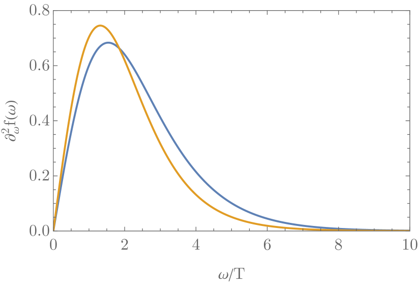
Figure 2: The figure shows the 0-eigenmode of the collision integral that includes consistent bosonic dynamics $I_{g^{\prime}}+I_{c_{D}}$. The blue line depicts the non-decaying eigenmode $\delta f_{0}(\omega)$ such that $I_{g^{\prime}}[\delta f_{0}]+I_{c_{d}}[I_{B}[\delta f_{0}]]/c_{d}=0$. The orange line depicts $\partial_{\omega}^{2}\bar{f}(\omega)$.

This mode has a very similar to $\partial_{\omega}^{2}\bar{f}(\omega)$ in profile, but unlike in the case of thermalized boson, it’s eigenvalue is very small. All the other eigenmodes that we recover have finite eigenvalues and therefore will decay much faster. We associate the 0-eigenvalue mode that we obtained with the energy conservation law that is present in the model when the boson dynamics is present. Unlike the case of the thermalized boson, the boson field does no longer serve as a heat bath for the fermions, but dynamically exchanges energy with the fermion. Moreover, since the bosons are only coupled to fermions and potential disorder, the conservation of energy should be applicable for the whole system. Thus there should be a collective fermion-boson mode that would nullify the collision integral due to the energy conservation. Introduction of additional thermal baths, which are inevitably present in any real setup, will drive the eigenvalue of this mode away from $0$.

Due to a big similarity between the 0-eigenvalue mode of the collision integral, we propose a simple phenomenological model that will capture those features. We propose to treat the 0-eigenvalue mode simply as $\partial_{\omega}^{2}\bar{f}(\omega)$. For the case $\nu\neq 0$, the eigenvalue then interpolates as

$$I_{g^{\prime}}[\partial_{\omega}^{2}\bar{f}]+\frac{I_{c_{d}}[I_{B}[\partial_{\omega}^{2}\bar{f}]]}{i\nu+c_{d}}=-\frac{g^{\prime 2}k_{F}T}{4\pi v_{F}}\frac{i\nu/c_{d}}{1+i\nu/c_{d}}\partial_{\omega}^{2}\bar{f}.$$ (117)

Thus the eigenvalue has to be proportional to $i\nu$, and therefore is just another term that contributes to a dynamic term. Moreover, since it is also proportional to $T$, at low temperatures it will be just a small correction to $a(\omega,T)$, and therefore can be neglected. Notice, however, that the terms that arise from the structure of $K$ and $k_{C}$ are the only terms that carry the value of the constant $c_{c}$ explicitly in them. Thus, the value of $c_{d}$ can be inferred from experiment if one can conduct a precise enough experiment that would provide information on the $m=0$ harmonic dynamics. In the section below we will show that the Joule heating-related non-linear response in the optical limit provides an opportunity to tackle the information about the density harmonic dynamics experimentally, and thus infer the value of $c_{d}$.

To summarize our insights in the dynamic structure of the fermion $\delta f_{0}$ harmonic behavior, we describe again a phenomenological model that we adopt for the evolution of $\delta f_{0}$ harmonics, in particular for the cases when $\delta f_{0}\sim\partial_{\omega}^{2}\bar{f}(\omega)$. The dynamic term in Eq. (108) takes a form

$$A[i\nu\delta f_{0}]=i\nu\,a(\omega,T)\delta f_{0}.$$ (118)

The collision integral term in the RHS of Eq. (108) takes a form of

$$I_{g^{\prime}}[\partial_{\omega}^{2}\bar{f}]+\frac{I_{c_{d}}[I_{B}[\partial_{\omega}^{2}\bar{f}]]}{i\nu+c_{d}}=-\Gamma_{0}\,\partial_{\omega}^{2}\bar{f},$$ (119)

where

$$\Gamma_{0} =\frac{g^{\prime 2}k_{F}T}{4\pi v_{F}},\quad\delta f_{B}=0,$$ (120)

$$\Gamma_{0} =0,\quad\delta f_{B}\neq 0,$$ (121)

With this relatively simple phenomenological model motivated by our numerical study, we proceed to construct the perturbation theory in electric field in the next section.

VI Perturbation theory in electric field

We proceed towards construction of the solution to the kinetic equations for fermions $\delta f$ and bosons $\delta f_{B}$ by the means of perturbation theory. We will consider the solution order by order and in the process we will recover a known result for linear response, analyze the structure of the collision integral terms with enabled and disabled dynamics. Eventually construct the description for the third-order response (second order is nullified by inversion symmetry) and analyze the leading order scaling with temperature. Additionally, We will compare the strange metal higher order responses to the Fermi-liquid responses. We will show that the strange metal response grows large as $T\rightarrow 0$ with an extra power of $1/T$, which appears due to the non-analytic behavior of the model at $\omega=0$ at $T=0$. While performing the analysis, we will differentiate between the non-linear responses coming from the energy harmonic excitations (Joule heating), and other types of non-linear response. As a side product of our calculations, we will also obtain the expression for linear resistivity which is consistent with the previous results that involve the model of a critical Fermi-surface [20, 21, 22, 36].

First we organize the perturbation theory by expanding the harmonics $\delta f_{m}$ in the powers of $\mathcal{E}$, where $\mathcal{E}$ is related to electric field components by $\mathcal{E}=E_{x}+iE_{y}$:

$$\delta f_{m}(\omega)=\sum_{n=1}^{\infty}\delta f_{m}^{(n)}(\omega).$$ (122)

We use the superscript to denote the order of the perturbation, so the term $\delta f_{m}^{(n)}(\omega)$ is a homogeneous polynomial of $\mathcal{E}$ and $\mathcal{E}^{*}$ of power $n$.

We are interested in the first non-trivial non-linear response, which is expected to be a third order response. Thus we are mostly interested in the structure of $\delta f^{(3)}$ and all the lower orders. To obtain the relevant equations we substitute the expansion for $\delta f_{m}$ in Eq. (122) into Eqs. (96) and (108) and expand in the powers of electric field the fermion kinetic equations for $m\neq 0$ harmonics:

$$[i\partial_{t}\,a(\omega,T)+2\Gamma+2g(\omega,T)]\delta f_{m}^{(1)}(\omega) =-\frac{ev_{F}}{2}\,\partial_{\omega}\bar{f}(\omega)(\mathcal{E}^{*}\delta_{1,m}+\mathcal{E}\delta_{-1,m}),$$ (123)

$$[i\partial_{t}\,a(\omega,T)+2\Gamma+2g(\omega,T)]\delta f_{m}^{(3)}(\omega) =-\frac{ev_{F}}{2}\,\partial_{\omega}(\mathcal{E}^{*}\delta f_{m-1}^{(2)}(\omega)+\mathcal{E}\delta f_{m+1}^{(2)}(\omega))+I^{\prime(3)}_{\mathrm{nl}},$$ (124)

where term $I^{\prime}_{\mathrm{nl}}$ is the non-linear correction in the third order that comes from Eq. (97) and, particularly, in the third order takes a form

$$I_{\mathrm{nl}}^{\prime(3)}=-\frac{g^{\prime 2}k_{F}}{v_{F}}\int\frac{d\Omega}{2\pi}B(\Omega)\left[2\,\delta f_{B0}^{(2)}(\Omega)+\delta f_{0}^{(2)}(\omega+\Omega)\right]\delta f_{m}^{(1)}(\omega).$$ (125)

For the higher responses one will have to consider all the non-linear correction terms shown in Appendix A instead of just focusing on the leading order of corrections described in Eq. (97).

Following our discussion in Sec. V, the evolution of the density harmonics $\delta f_{0}$ is governed by an equation of a different form. We expand it in the orders of perturbation up to $n=2$ and obtain

$$i\nu\,a(\omega,T)\delta f_{0}^{(2)}(\omega)-I[\delta f_{0}^{(2)}(\omega)]=-\frac{ev_{F}}{2}\,\partial_{\omega}(\mathcal{E}\delta f_{1}^{(1)}+\mathcal{E}^{*}\delta f_{-1}^{(1)}),$$ (126)

The collision integral $I$ is given by $I=I_{g^{\prime}}$ for thermalized boson or $I=I_{g^{\prime}}+I_{c_{d}}[I_{B}]$ for a dynamic boson, as in Eq. (106). Note that in the orders of perturbation higher than $n=2$ there will be numerous non-linear corrections to this equations which will turn out to be important when computing higher order responses.

Finally, we consider the source of electric field $\mathbf{E}$ of the form

$$\mathbf{E}=\sum_{i}\mathbf{E}_{\nu_{i}}e^{i\nu_{i}t},$$ (127)

where $\mathbf{E}_{\nu_{i}}$ are the space-independent coefficients and use the expanded equations in Eqs. (123), (124), and (126) to construct the perturbation in $\delta f$ and later use $\delta f$ solution to compute the response current $\mathbf{j}$.

VI.1 Linear perturbation in electric field

As the first step, we compute the perturbation in $\delta f$ up to a linear in $E$ term, which we denoted as $\delta f^{(1)}$:

$$\delta f^{(1)}=\sum_{m=-\infty}^{\infty}\delta f_{m}^{(n)}e^{im\theta_{k}}.$$ (128)

Since $\delta f_{\pm 1}^{0}=0$ by definition, the density harmonic $m=0$ is not perturbed in the first order, and therefore $\delta f_{0}^{1}=0$. Thus, all the dynamics of $\delta f^{(1)}$ is captured by harmonics $\delta f^{(1)_{\pm 1}}$ described by Eq. (123). It is useful to multiply Eq. (123) by $e^{im\theta_{k}}$ and sum over $m$ to reconstruct the equation for $\delta f^{(1)}$:

$$[i\nu_{i}\,a(\omega,T)+2\Gamma+2g(\omega,T)]\,\,\delta f^{(1)}=-ev_{F}\,(\mathbf{E}_{\nu_{i}}\cdot\hat{\mathbf{k}})\,\partial_{\omega}\bar{f}.$$ (129)

The solution to the equation above is

$$\delta f^{(1)}(\omega)=-ev_{F}\sum_{i}(\mathbf{E}_{\nu_{i}}\cdot\hat{\mathbf{k}})\,e^{i\nu_{i}t}\,W(\omega,\nu_{i},T)\frac{\partial\bar{f}}{\partial\omega}(\omega),$$ (130)

where the transfer function $W$ is

$$W(\omega,\nu,T)=\frac{1}{i\nu\,a(\omega,T)+2\Gamma+2g(\omega,T)}.$$ (131)

Note that under our assumptions, the dominant term in the denominator of $W(\omega,\nu,T)$ at low temperatures and $\nu\ll T$ is $\Gamma$, which does not depend on temperature.

One of the properties of the $\delta f^{(1)}(\omega)$ which will become important in the next subsection, is the symmetry of the solution with respect to $\omega\rightarrow-\omega$. Since $g(\omega,T)$, $a(\omega,T)$, and $\partial_{\omega}\bar{f}$ are symmetric functions under $\omega\rightarrow-\omega$, $\delta f^{(1)}$ is symmetric under $\omega\rightarrow-\omega$.

We use the solution for $\delta f^{(1)}$ in Eq. (130) in the following subsections to compute linear conductivity and to compute higher orders of the perturbation $\delta f^{(n)}$ in the following subsections.

VI.2 Second order perturbation in electric field

In the second order of perturbation in $\mathbf{E}$ one, in general, would expect two types of excitations: $\delta f_{\pm 2}^{(2)}$ and $\delta f_{0}^{(2)}$, which are the ”tensor” $m=2$ and the ”particle density” $m=0$ harmonic. The corresponding equations for these harmonics are derived from Eqs. (124) and (126). Since $\delta f_{\pm 3}^{(1)}=0$, it is particularly easy to construct the equations for $\delta f_{\pm 2}^{(2)}$:

$$[i\nu\,a(\omega,T)+2\Gamma+2g(\omega,T)]\delta f_{2}^{(2)} =-\frac{ev_{F}}{2}\mathcal{E}^{*}\partial_{\omega}\delta f_{1}^{(1)}$$ (132)

$$[i\nu\,a(\omega,T)+2\Gamma+2g(\omega,T)]\delta f_{-2}^{(2)} =-\frac{ev_{F}}{2}\mathcal{E}\partial_{\omega}\delta f_{-1}^{(1)}$$ (133)

The solution to these equations can be constructed in the analogous way to the solution in Eq. (130) and we obtain

$$\delta f_{2}^{(2)}=\frac{e^{2}v_{F}^{2}}{4}\sum_{i,j}\mathcal{E}^{*}_{\nu_{i}}\mathcal{E}^{*}_{\nu_{j}}e^{i\nu_{ij}t}W(\omega,\nu_{ij},T)\frac{\partial}{\partial\omega}\left[W(\omega,\nu_{i},T)\frac{\partial\bar{f}}{\partial\omega}\right]$$ (134)

where $\nu_{ij}=\nu_{i}+\nu_{j}$. Analogous expression for $\delta f_{-2}^{(2)}$, but it involves to factors of $\mathcal{E}$ instead of two factors of $\mathcal{E}^{*}$ in Eq. (134).

Now we proceed towards a similar construction for the density harmonic $\delta f_{0}^{(2)}$, which, however, will be more involved. At first we need to use the explicit solution we constructed for $\delta f^{(1)}$ to justify the approximations we have implemented in Sec. V and show that the structure of the second order perturbation of a density harmonic has a rather simple profile. Note that in previous subsection we showed that $\delta f^{(1)}$ is a symmetric function of $\omega$. Thus the source term in Eq. (126) is an anti-symmetric function of $\omega$, which implies that $\delta f^{2}_{0}$ will also be an anti-symmetric function of $\omega$. Therefore the reduction of $A[\partial_{t}\delta f_{0}]$ to $a(\omega,T)\,\partial_{t}\delta f_{0}$ is justified in our context due to the anti-symmetry of the argument. Let’s take the closer look at the $\omega$-profile of the RHS source term in Eq. (126). The source has a form $\partial_{\omega}\delta f^{(1)}_{\pm 1}$, where function $\delta f^{(1)}_{\pm 1}$ is

$$\delta f^{(1)}_{\pm 1}\sim W(\omega,\nu,T)\partial_{\omega}\bar{f}=\frac{\partial_{\omega}\bar{f}}{i\nu a(\omega,T)+\Gamma+g(\omega,T)}.$$ (135)

The $\omega$ derivative of $\delta f^{(1)}_{\pm 1}$ involves two terms: $W(\omega,\nu,T)\partial_{\omega}^{2}\bar{f}$ and $\partial_{\omega}W(\omega,\nu,T)\partial_{\omega}\bar{f}$. In the first term, as we mentioned above, $\Gamma$ is dominant in the denominator and therefore we can approximate the term as $W(\omega,\nu,T)\partial_{\omega}^{2}\bar{f}\sim\partial_{\omega}^{2}\bar{f}/\Gamma$. The second term involves a derivative of $W$ and can be approximated as $\partial_{\omega}W(\omega,\nu,T)\partial_{\omega}\bar{f}\sim(i\nu\partial_{\omega}a+\partial_{\omega}g)\partial_{\omega}\bar{f}/\Gamma^{2}$. By comparing the $T>0$ expressions for $i\nu\partial_{\omega}a$ and $\partial_{\omega}g$ in Eqs. (73) and (79) correspondingly, we see that under assumption of $\nu\ll T$ the derivative of $g$ dominates over the derivative of $a$. Additionally, we see that the derivative of $g$ is a constant factor multiplied by $1-2\bar{f}(\omega)$. Since $(1-2\bar{f}(\omega))\partial_{\omega}\bar{f}\sim\partial_{\omega}^{2}\bar{f}$, the second term is also proportional to $\partial_{\omega}^{2}\bar{f}$ in the leading order. Since the source therm in the RHS of Eq. (126) has a profile $\sim\partial_{\omega}^{2}\bar{f}$, we can apply the approximate treatment of the $m=0$ harmonic of the collision integral developed in Sec. V and Eq. (126) simplifies to

$$[i\nu\,a(\omega,T)+\Gamma_{0}(T)]\delta f_{0}^{(2)}(\omega)=-\frac{ev_{F}}{2}\,\partial_{\omega}(\mathcal{E}\delta f_{1}^{(1)}+\mathcal{E}^{*}\delta f_{-1}^{(1)}),$$ (136)

where according to our model constructed in Sec. V, $\Gamma_{0}(T)=g^{\prime 2}k_{F}T/4\pi v_{F}$ if the boson is in thermal equilibrium and $\Gamma_{0}=0$ when the boson dynamics is fully consistent with the fermion dynamics. Eq. (136) can be easily solved, the solution with explicit dependence on $\mathbf{E}$ is

$$\delta f_{0}^{(2)}=\frac{e^{2}v_{F}^{2}}{2}\sum_{i,j}(\mathbf{E}_{\nu_{i}}\cdot\mathbf{E}_{\nu_{j}})\,e^{i\nu_{ij}t}W_{0}(\omega,\nu_{ij},T)\frac{\partial}{\partial\omega}\left[W(\omega,\nu_{i},T)\frac{\partial\bar{f}}{\partial\omega}\right],$$ (137)

where $\nu_{ij}=\nu_{i}+\nu_{j}$ and the factor $W_{0}$ for an $m=0$ harmonics is

$$W_{0}(\omega,\nu,T)=\frac{1}{i\nu a(\omega,T)+\Gamma_{0}(T)}.$$ (138)

Note the similarity in the perturbative expansion structure for $\delta f_{0}^{(2)}$ and $\delta f_{\pm 2}^{(2)}$ harmonics. The only difference is the choice of the factor: $W$ for $m\neq 0$ and $W_{0}$ for $m=0$.

The density harmonic $m=0$ is related to the particle density and the energy density in the system. Thus, the non-linear responses that involve the excitation of the $m=0$ harmonic have a physical meaning of the non-linear responses coming from the change of energy density in the system. This effect, when the change of energy density is positive, is associated with the Joule heating of the system by the external driving heat. Thus, the non-linear response contributions that arise from the excitation of the density harmonics should be regarded as the joule heating effect. Other contributions should be regarded just as ordinary non-linear effects. A complete solution for $\delta f^{(2)}$ can be written as

$$\delta f^{(2)}=\delta f_{0}^{(2)}+\delta f_{2}^{(2)}e^{2i\theta_{k}}+\delta f_{-2}^{(2)}e^{-2i\theta_{k}}.$$ (139)

Thus, we have ordinary non-linear terms and the Joule heating terms included and in the following sub-sections we will analyze the consequences for both contributions.

VI.3 Third order perturbation in electric field

The third order response tackles harmonics with $m=\pm 3$ and $m=\pm 1$. Since we are interested in eventually computing the currents from the perturbations, we will focus on deriving the expressions for $m=\pm 1$ harmonics, which is the only harmonics that carries current in a spherically symmetric system. The equations that govern the evolution of $\delta f_{\pm 1}^{(3)}$ can be obtained from Eq. (124), which is

$$[i\nu\,a(\omega,T)+2\Gamma+2g(\omega,T)]\delta f_{m}^{(3)}(\omega)=-\frac{ev_{F}}{2}\,\partial_{\omega}(\mathcal{E}^{*}\delta f_{m-1}^{(2)}(\omega)+\mathcal{E}\delta f_{m+1}^{(2)}(\omega))+I^{\prime(3)}_{\mathrm{nl}},$$ (140)

where $m=\pm 1$. The non-linear correction has a form

$$I_{\mathrm{nl}}^{\prime(3)}=-\frac{g^{\prime 2}k_{F}}{v_{F}}\int\frac{d\Omega}{2\pi}B(\Omega)\left[2\,\delta f_{B0}^{(2)}(\Omega)+\delta f_{0}^{(2)}(\omega+\Omega)\right]\delta f_{m}^{(1)}(\omega),$$ (141)

where in thermalized boson dynamics case $\delta f_{B0}^{(2)}=0$, and when the dynamics is accounted for,

$$\delta f_{B0}^{(2)}=\frac{1}{i\nu+c_{d}}\frac{g^{\prime}c^{2}k_{F}^{2}}{2v_{F}^{2}}\int\frac{d\omega}{2\pi}\int\frac{d\hat{k}}{2\pi}\frac{1}{\Omega}\left(1-f(\omega-\Omega)-f(\omega+\Omega)\right)\times\left(\delta f_{0}^{(2)}(\omega)-C(\Omega)\,\partial_{t}\delta f_{0}^{(2)}(\omega)\right).$$ (142)

Notice that due to a non-linear nature of $I_{\mathrm{nl}}^{\prime 3}$ does not contain any factors of $\delta f^{(3)}$. The non-linear correction only contains the terms that depend on $\delta f_{0}^{(2)}$ and $\delta f_{m}^{(1)}$, which have already been obtained by the means of the perturbation theory. The same conclusion will be applicable to all non-linear corrections that come from the collision integral, and thus we argue that the non-linear corrections to the collision integral only play the role of additional sources in the equations of the type of Eq. (140) and analogous to it. In the rest of the subsections we solve Eq. (140) with all the sources included and find that in case of the strange metal the sources originating non-linear corrections have no significant impact on the non-linear response. Notice, however, that the non-linear correction term solely arises from the excitation of $m=0$ harmonics for bosons and fermions, and thus has to be attributed to the effects of the Joule heating. Therefore, the ordinary non-linear response term should be computed with $\delta f_{0}=\delta f_{B0}=0$. Therefore, we have to make a distinction between the different types of non-linear responses and and to achieve this we denote the perturbations associated to Joule heating as $\delta f_{J,\pm 1}^{(3)}$, and the perturbations associated with ordinary non-linear response as just $\delta f^{(3)}_{\pm 1}$. As was mentioned above, the ordinary perturbations come from Eq. (140) with an assumption that no density harmonics are perturbed and result is

$$\delta f_{1}^{(3)}=-\frac{e^{3}v_{F}^{3}}{8}\sum_{i,j,l}\mathcal{E}^{*}_{\nu_{i}}\mathcal{E}^{*}_{\nu_{j}}\mathcal{E}_{\nu_{l}}e^{i\nu_{ijl}t}W(\omega,\nu_{ijl},T)\frac{\partial}{\partial\omega}\left[W(\omega,\nu_{ij},T)\frac{\partial}{\partial\omega}\left[W(\omega,\nu_{i},T)\frac{\partial\bar{f}}{\partial\omega}\right]\right],$$ (143)

and $\delta f_{-1}^{(3)}=(\delta f_{-1}^{(3)})^{*}$.

To compute the Joule heating-related response $\delta f_{J,\pm 1}^{(3)}$ we split the expression into three terms $\delta f_{J,\pm 1}^{(3)}$ based on the origin of the source of the term in Eq. (140):

$$\delta f_{J,\pm 1}^{(3)}=\delta f_{J-\mathrm{main},\pm 1}^{(3)}+\delta f_{J-\mathrm{nl},\pm 1}^{(3)}+\delta f_{J-\mathrm{bos,nl},\pm 1}^{(3)}.$$ (144)

The term $\delta f_{J-\mathrm{main},\pm 1}^{(3)}$ we associate with the ”main” contribution that is present even when $I^{\prime(3)}_{\mathrm{nl}}=0$. The term $\delta f_{J-\mathrm{nl}}$ we attribute to the source coming from a non-linear correction that is associated with $\delta f_{0}^{(2)}$ in Eq. (141), present even when $\delta f_{B0}=0$. Finally, the term $\delta f_{J-\mathrm{bos,nl},\pm 1}^{(3)}$ we associate with the non-linear contribution of the bosonic dynamics $\delta f_{B0}^{(2)}$ in the Eq. (141). The corresponding expression for main contribution is

$$\delta f_{J-\mathrm{main},1}^{(3)}=-\frac{e^{3}v_{F}^{3}}{4}\sum_{i,j,l}\mathcal{E}^{*}_{\nu_{l}}(\mathbf{E}_{\nu_{j}}\cdot\mathbf{E}_{\nu_{i}})\,e^{i\nu_{ijl}t}W(\omega,\nu_{ijl},T)\frac{\partial}{\partial\omega}\left[W_{0}(\omega,\nu_{ij},T)\frac{\partial}{\partial\omega}\left[W(\omega,\nu_{i},T)\frac{\partial\bar{f}}{\partial\omega}\right]\right].$$ (145)

The non-linear correction from a thermalized boson contribution is obtained by setting $\delta f_{B0}^{(2)}=0$ in Eq. (141) along with using Eq. (137) for $\delta f_{0}^{(2)}$ and has a form

$$\delta f_{J-\mathrm{nl},1}^{(3)}=-\frac{g^{\prime 2}k_{F}}{4\pi v_{F}}\frac{e^{3}v_{F}^{3}}{4}\sum_{\nu_{i},\nu_{j},\nu_{l}}\mathcal{E}^{*}_{\nu_{l}}(\mathbf{E}_{\nu_{j}}\cdot\mathbf{E}_{\nu_{i}})\,e^{i\nu_{ijl}t}\times\\ \times W(\omega,\nu_{ijl},T)W(\omega,\nu_{l},T)W_{0}(\omega,\nu_{ij},T)W(\omega,\nu_{i},T)\left(\frac{\partial f}{\partial\omega}(\omega)\right)^{2}.$$ (146)

The non-linear contribution from boson dynamics is obtained by substituting Eqs. (142) and (137) into Eq. (141) and setting $\delta f_{0}^{(2)}=0$ and becomes

$$\delta f_{J-\mathrm{bos,nl},1}^{(3)}=\frac{g^{\prime 2}c^{2}k_{F}^{3}}{4\pi v_{F}^{3}(i\nu+c_{d})}\frac{e^{3}v_{F}^{3}}{48\pi T}\left(\ln\left(\frac{c_{d}T}{m^{2}}\right)+\gamma_{b}\right)\times\\ \times\sum_{\nu_{i},\nu_{j},\nu_{l}}\mathcal{E}^{*}_{\nu_{l}}(\mathbf{E}_{\nu_{j}}\cdot\mathbf{E}_{\nu_{i}})\,e^{i\nu_{ijl}t}W(\omega,\nu_{ijl},T)W_{0}(0,\nu_{ij},T)W(0,\nu_{i},T)W(\omega,\nu_{l},T)\frac{\partial\bar{f}}{\partial\omega}(\omega)$$ (147)

with $\gamma_{b}\approx 0.91$. Even though the terms $\delta f_{J-\mathrm{nl},1}^{(3)}$ and $\delta f_{J-\mathrm{bos,nl},1}^{(3)}$ seem to have a rather different from $\delta f_{J-\mathrm{main},1}^{(3)}$ structure in the first glance, they are still strongly peaked functions at $\omega=0$ of width $\omega\sim T$. We will show that their contributions into current look alike to the contribution coming from $\delta f_{J-\mathrm{main},1}^{(3)}$.

From the expressions for the perturbation in Eq. (143) we can infer a structure of non-linear responses in this model. Every extra order of non-linear response comes with a term proportional to electric field and the factor of $W\partial_{\omega}$. The structure of the responses that excite the density harmonic is more complicated: when we perturb the density harmonic $m=0$, the additional factor becomes $W_{0}\partial_{\omega}$, and several extra corrections from non-linear terms take place too. We will explore the structure of the higher order responses in a greater detail later in this section and meanwhile focus on computing the current responses for the linear and 3rd order responses.

VI.4 Currents in linear and third order responses

Some of the basic observables to study with the perturbation theory include linear conductivity and higher order conductivities. We, in particular, are interested in computing the current produced by perturbations $\delta f^{(1)}$ and $\delta f^{(3)}$ to extract the features of the temperature dependence of the response. The corresponding currents can be obtained with

$$\mathbf{j}^{(n)}=ek_{F}\int_{-\infty}^{+\infty}\frac{d\omega}{2\pi}\int_{0}^{2\pi}\frac{d\hat{\mathbf{k}}}{2\pi}\hat{\mathbf{k}}\,\delta f^{(n)}(\omega).$$ (148)

We start from recovering an expected result for the linear response for $\mathbf{j}^{(1)}$ and famous linear in $T$ conductivity. We substitute the expression for $\delta f^{(1)}$ from Eq. (130) into Eq. (148) and obtain

$$\mathbf{j}^{(1)}=-\frac{e^{2}v_{F}k_{F}}{2}\sum_{i}\mathbf{E}_{\nu_{i}}\,e^{i\nu_{i}t}\int_{-\infty}^{+\infty}\frac{d\omega}{2\pi}\,W(\omega,\nu_{i},T)\frac{\partial\bar{f}}{\partial\omega}$$ (149)

Now it is instructive to show the connection between the non-analytical structure of $a$ and $g$ at $T=0$ and the divergent responses. A typical next step in evaluating the integral like in Eq. (149) in Fermi-liquid theory will involve taking a limit $T\rightarrow 0$ that turns $\partial_{\omega}\bar{f}$ into a $\delta$-function, and then evaluating the integral. let’s formally perform that step and analyze the expression:

$$\mathbf{j}^{(1)}=\frac{e^{2}v_{F}k_{F}}{4\pi}\sum_{i}\frac{\mathbf{E}_{\nu_{i}}e^{i\nu_{i}t}}{i\nu_{i}a(0,0)+2\Gamma+2g(0,0)}.$$ (150)

On our way here, we several times mentioned the expressions $a(\omega,T=0)$ and $g(\omega,T=0)$, which can be found in Eqs. (74) and (80) correspondingly. Notice that $g(0,0)=0$ is well-defined, however $a(\omega\rightarrow 0,0)$ is logarithmic-divergent, which is a smoking gun of the singularities at $T=0$ and potential extra divergences in the higher order responses. Indeed, the structure of $a(\omega,T>0)$ contains a logarithmic divergence of $a(\omega,T)\sim\ln(T_{\Lambda}/T)$ for all $\omega\lesssim T$. Thus the naive limit $T\rightarrow 0$ that has been taken in Eq. (150) is an illegal operation. We will have to be more careful when taking the limits and will need to study the structure of the integrands. When we use full expressions for $a(\omega,T)$ and $g(\omega,T)$, we can see that function $\partial_{\omega}\bar{f}$ is a sharp peak of width $T$. Since $\Gamma$ is a dominant term in $W(\omega,\nu,T)$, the function $W$ does not have any serious peaks or discontinuities in the vicinity of $\omega\sim T$. Thus, to estimate the values of the integral, we can substitute $\omega=T$ into $a(\omega,T)$ and $g(\omega,T)$ when evaluating the integral in Eq. (149). Assuming that the cotribution $g(\omega\sim T,T)\ll\Gamma$, we can expand $W(\omega,\nu_{i},T)$ in Eq. (149) and we obtain

$$\mathbf{j}^{(1)}=\frac{e^{2}v_{F}k_{F}}{4\pi}\sum_{i}\frac{\mathbf{E}_{\nu_{i}}e^{i\nu_{i}t}}{i\nu_{i}\tilde{a}(T)+2\Gamma+2\tilde{g}(T)},$$ (151)

where up to a leading order

$$\tilde{a}(T) =-\int_{-\infty}^{+\infty}d\omega\,\frac{\partial\bar{f}}{\partial\omega}(\omega)\,a(\omega,T)=\frac{g^{\prime 2}k_{F}}{8\pi^{2}v_{F}}\ln\left(\frac{\omega_{\Lambda}}{T}\right),$$ (152)

$$\tilde{g}(T) =-\int_{-\infty}^{+\infty}d\omega\,\frac{\partial\bar{f}}{\partial\omega}(\omega)\,g(\omega,T)=\frac{g^{\prime 2}k_{F}}{8\pi v_{F}}T\ln\left(\frac{4c_{d}T}{em^{2}}\right)=\gamma(T)\frac{g^{\prime 2}k_{F}}{8\pi v_{F}}T.$$ (153)

The boson mass $m^{2}\approx\pi c_{d}T/\ln(T_{\Lambda}/T)$, the function $\gamma(T)$ is a very slowly changing function of $T$ due to the double logarithm term

$$\gamma(T)=\ln\left(\frac{4}{\pi e}\right)+\ln\ln\left(\frac{T_{\Lambda}}{T}\right).$$ (154)

Considering the case when $T_{\Lambda}$ being very, large, in the interval $T\in(10^{-2}T_{\Lambda},10^{-10}T_{\Lambda}$), the value of $\gamma(T)$ changes in the interval of $(1,1.5)$, which sets it to be some constant $\sim 1$ for any physically relevant scenario. The resulting linear conductivity becomes

$$\sigma_{\mathrm{nFL}}(\nu,T)=\frac{e^{2}v_{F}k_{F}/4\pi}{i\nu\,\tilde{a}(T)+2\Gamma+2\tilde{g}(T)}.$$ (155)

which can be equivalently written as a linear resistivity of the form

$$\rho_{\mathrm{nFL}}(\nu,T)=\frac{1}{\sigma_{\mathrm{nFL}}(\nu,T)}=\rho_{0}+i\nu\beta_{\rho}\ln\left(\frac{T_{\Lambda}}{T}\right)+\alpha_{\rho}T,$$ (156)

which is exactly Eq. (5) up to restoring the factors of $\hbar$ and $k_{b}$ with the coefficients being defined as

$$\rho_{0}=\frac{8\pi\Gamma}{e^{2}v_{F}k_{F}},\quad\beta_{\rho}=\frac{g^{\prime 2}}{2\pi e^{2}v_{F}^{2}},\quad\alpha_{\rho}=\gamma(T)\frac{g^{\prime 2}}{e^{2}v_{F}^{2}}=2\pi\gamma(T)\beta_{\rho}.$$ (157)

This result reproduces the previous diagrammatic calculations performed in [21, 22] and, additionally, correctly predicts the frequency-dependent part of the conductivity conjectured in [36]. Additionally, we receive the plankian scattering rate $1/\tau_{\mathrm{Pl}}=\gamma(T)/\ln(T_{\Lambda}/T)\,\cdot k_{B}T/\hbar$.

The calculation above is valid only for small enough temperatures where $\alpha_{\rho}T\ll\rho_{0}$, and the regime of large temperatures has to be computed separately. In the regime of large temperature $g(\omega,T)$ is the only dominant term in Eq. (149), and the regime of large temperatures leads to a different expression for a slope $\gamma(T)$ that, in this case, we denote $\gamma_{\Gamma\gg T}(T)$. After numerically evaluating the integral in Eq. (149) in the large temperature limit we find that for a physically relevant values of $\gamma(T)$ given by Eq. (154) lead to a numerically robust relation $\gamma_{\Gamma\gg T}(T)\approx 1.03\gamma(T)+0.12$ for $\gamma(T)$ ranging from 1 to 3. Thus, even though the cross-over at $\alpha_{\rho}T\sim\rho_{0}$ exists, the actual change of slope is insignificant and can be ignored.

Away from the critical point the values of $g(\omega,T)$ and $a(\omega,T)$ are described by Eqs. (81) and (76) correspondingly. When substituted into the equation for current in Eq. (149), it results in

$$\rho_{\mathrm{FL}}=\frac{1}{\sigma_{\mathrm{FL}}}=\rho_{0}+i\nu\beta_{\rho,\mathrm{FL}}+\kappa_{\rho}T^{2},$$ (158)

where the coefficients are

$$\rho_{0}=\frac{8\pi\Gamma}{e^{2}v_{F}k_{F}},\quad\beta_{\rho,\mathrm{FL}}=\frac{4\pi}{e^{2}v_{F}k_{F}}\left[1+\frac{g^{\prime 2}k_{F}}{8\pi^{2}v_{F}}\ln\left(\frac{c^{2}\Lambda_{q}^{2}}{\Delta^{2}}\right)\right],\quad\kappa_{\rho}=\frac{2\pi g^{\prime 2}c_{d}}{e^{2}v_{F}^{2}\Delta^{2}}.$$ (159)

In ordinary two-dimensional Fermi-liquids the scattering rates are such that $g_{\mathrm{FL}}(\omega,T)=\gamma_{\mathrm{FL}}(\pi^{2}T^{2}+\omega^{2})/\varepsilon_{F}$, which instantly leads to Eq. (4) ($\gamma_{\mathrm{FL}}$ is a dimensionless number of the order of $\sim 1$). In the vicinity of QCP $\gamma_{\mathrm{FL}}$ grows as the boson gap $\Delta$ approaches 0, from the expression for $\kappa_{\rho}$ we obtain

$$\gamma_{\mathrm{FL}}(\Delta)=\frac{3}{32\pi^{3}}\frac{c^{2}}{v_{F}^{2}}\left(\frac{g^{\prime 2}k_{F}}{v_{F}}\right)^{2}\frac{T_{F}^{2}}{\Delta^{2}}.$$ (160)

Since we expect $g^{\prime 2}k_{F}/v_{F}\sim 1$ due to the universal resistance scaling [34], we arrive to Eq. (4) again.

Now we proceed towards computing the higher order current responses. We focus on the first non-vanishing current $\mathbf{j}^{(3)}$, since $\mathbf{j}^{(2)}$ vanishes by inversion symmetry. We will consider both the current related to ordinary non-linear response $\mathbf{j}^{(3)}$ and the current associated with the Joule heating $\mathbf{j}^{(3)}_{J}$. To obtain $\mathbf{j}^{(3)}$ we start with substituting our solution for $\delta f^{(3)}_{\pm 1}$ from Eq. (143) into the current equation in Eq. (148), which results in

$$\mathbf{j}^{(3)}=-\frac{e^{3}v_{F}^{3}k_{F}}{8}\int\frac{d\omega}{2\pi}\sum_{i,j,l}\hat{\mathbf{k}}^{a}E^{b}_{\nu_{l}}E^{c}_{\nu_{j}}E^{d}_{\nu_{i}}\Delta_{a,bcd}\,e^{i\nu_{ijl}t}W(\omega,\nu_{ijl},T)\frac{\partial}{\partial\omega}\left[W(\omega,\nu_{ij},T)\frac{\partial}{\partial\omega}\left[W(\omega,\nu_{i},T)\frac{\partial\bar{f}}{\partial\omega}\right]\right].$$ (161)

In the equation above $\nu_{ijl}=\nu_{i}+\nu_{j}+\nu_{l}$ and tensor $\Delta_{a,bcd}$ components are defined by

$$\Delta_{1,bcd}=\,\mathrm{Re}\,[u_{b}u_{c}^{*}u_{d}^{*}],\quad\Delta_{2,bcd}=-\,\mathrm{Im}\,[u_{b}u_{c}^{*}u_{d}^{*}]$$ (162)

Where components of a vector $u_{a}$ are given by $u_{a}=(1,i)$.

Before diving into the analysis and the integration of concrete expressions for the conductivity, we want to highlight a very generic and important role of $a(\omega)$ and $g(\omega)$ in creation of non-zero $\mathbf{j}^{(3)}$ and other higher order responses. Above we conjectured that all the higher order responses can be obtained by adding factors of $W$ and extra derivatives on $\omega$, similar to Eq. (161). To better understand the structure of that equation let’s integrate it by parts first to transform it to a form

$$\mathbf{j}^{(3)}=-\frac{e^{3}v_{F}^{3}k_{F}}{8}\int\frac{d\omega}{2\pi}\sum_{i,j,l}\hat{\mathbf{k}}^{a}E^{b}_{\nu_{l}}E^{c}_{\nu_{j}}E^{d}_{\nu_{i}}\Delta_{a,bcd}\,e^{i\nu_{ijl}t}\frac{\partial\bar{f}}{\partial\omega}W(\omega,\nu_{i},T)\frac{\partial}{\partial\omega}\left[W(\omega,\nu_{ij},T)\frac{\partial W}{\partial\omega}(\omega,\nu_{ijl},T)\right].$$ (163)

Notice that this expression would vanish if $W(\omega,\nu,T)$ did not depend on $\omega$. Thus, the presence of an $\omega$-dependence in the scattering rates, in particular, $g(\omega,T)$ is important for the presence of non-linear responses. In Fermi-liquids with $g(\omega,T)\sim\omega^{2}$ and the strange metals with $g(\omega,T)\sim\ln\;\mathrm{ch}\;(\omega/2T)$ the criterion is satisfied and the non-linear responses will be present. However, the strange metals and Fermi liquids have a main difference. in Fermi-liquids the derivatives of $g_{\mathrm{FL}}(\omega,T)$ are all small, since they are suppressed by $\varepsilon_{F}$. In contrast, strange metals $\omega$-dependence always comes in a form of $\omega/T$, which make the derivatives, and thus non-linear responses, diverge as $T\rightarrow 0$. To illustrate this divergence we fist showcase how these divergences arise from the non-analyticity of $g(\omega,T=0)$. We perform a naive computation the same way to the liner response current in Eq. (150) and obtain

$$\mathbf{j}^{(3)}=-\frac{e^{3}v_{F}^{3}k_{F}}{16\pi}\sum_{i,j,l}\hat{\mathbf{k}}^{a}E^{b}_{\nu_{l}}E^{c}_{\nu_{j}}E^{d}_{\nu_{i}}\Delta_{a,bcd}\,e^{i\nu_{ijl}t}\times\\ \times W(0,\nu_{i},0)\left[\frac{\partial W}{\partial\omega}(0,\nu_{ij},0)\frac{\partial W}{\partial\omega}(\omega,\nu_{ijl},0)+W(0,\nu_{ij},0)\frac{\partial^{2}W}{\partial\omega^{2}}(\omega,\nu_{ijl},0)\right].$$ (164)

Besides an already mentioned in Eq. (150) linear response problem related to a divergence of $a(\omega,T=0)$ as $\omega\rightarrow 0$ in the expression for $W(0,\nu,0)$, the expression for non-linear current in Eq. (164) has a larger divergence. The term $\partial_{\omega}^{2}W(0,\nu,0)$ contains a term proportional to $\partial_{\omega}^{2}g(0,0)$. However $g(\omega,T=0)=|\omega|$, and thus second derivative is singular and current $\mathbf{j}^{(3)}$ diverges. The divergence law can be extracted in exactly the same manner as in the linear response case: we first evaluate the integral over $\omega$ in Eq. (163) and then study the low temperature limit. In the leading order in $1/T$ we obtain

$$\mathbf{j}^{(3)}=\frac{e^{4}v_{F}^{3}k_{F}}{48\pi}\sum_{\nu_{b},\nu_{c},\nu_{d}}\hat{\mathbf{k}}^{a}E^{b}_{\nu_{l}}E^{c}_{\nu_{j}}E^{d}_{\nu_{i}}\Delta_{a,bcd}\,e^{i\nu_{ijl}t}\;\frac{g^{\prime 2}k_{F}}{8\pi v_{F}}\frac{1}{T}\times\\ \times\frac{1}{i\nu_{i}\tilde{a}(T)+2\Gamma+2\tilde{g}(T)}\frac{1}{(i\nu_{ijl}\tilde{a}(T)+2\Gamma+2\tilde{g}(T))^{2}}\frac{1}{i\nu_{ij}\tilde{a}(T)+2\Gamma+2\tilde{g}(T)},$$ (165)

which can be rewritten using known quantities from linear resistivity in Eq. (156) and results in non-linear conductivity of the form

$$\sigma^{(3)}_{\mathrm{nFL},a,bcd}(\nu_{b},\nu_{c},\nu_{d})=\frac{2\pi^{2}}{3e^{2}k_{F}^{2}}\frac{\alpha_{\rho}}{\gamma(T)T}\sigma_{\mathrm{nFL}}(\nu_{d},T)\,\sigma_{\mathrm{nFL}}^{2}(\nu_{bcd},T)\,\sigma_{\mathrm{nFL}}(\nu_{cd},T)\Delta_{a,bcd}.$$ (166)

As we expected, the conductivity is proportional to inverse temperature and since at small temperatures linear conductivity $\sigma_{\mathrm{nFL}}$ is constant, expression in Eq. (166) diverges at small temperatures as $1/T$. Even though the expression for non-linear conductivity was derived for small temperatures $T\ll\Gamma$, the expression above appears to be applicable for all the values of temperature with a good accuracy. The expression for $\sigma_{\mathrm{nFL}}^{(3)}$ for the regime of temperatures $T\gg\Gamma$ has an identical to Eq. (166) form with an overall coefficient in front of the expression being less by a factor of $\approx 17/20=0.85$.

A similar expression for non-linear conductivity to an expression in Eq. (166) can be derived for a Fermi liquid regime. In a similar manner to a derivation of an Eq. (158), we use the expressions for $a_{\mathrm{FL}}$ and $g_{\mathrm{FL}}$ given in Eqs. (76) and (81) instead of the non-Fermi liquid expressions for $a(\omega,T)$ and $g(\omega,T)$. The non-linear conductivity then becomes

$$\sigma_{\mathrm{FL},a,bcd}^{(3)}(\nu_{b},\nu_{c},\nu_{d})=\frac{16\pi^{3}}{e^{4}v_{F}k_{F}^{3}}\frac{g^{\prime 2}k_{F}c_{d}}{8\pi^{2}v_{F}\Delta^{2}}\sigma_{\mathrm{FL}}(\nu_{d},T)\sigma_{\mathrm{FL}}^{2}(\nu_{bcd},T)\sigma_{\mathrm{FL}}(\nu_{cd},T)\Delta_{a,bcd}.$$ (167)

In the ordinary Fermi liquids $g_{\mathrm{FL}}(\omega,T)=\gamma_{\mathrm{FL}}(\pi^{2}T^{2}+\omega^{2})/\varepsilon_{F}$, which results in the expression similar to the Fermi liquid result in Sec. I ($\gamma_{\mathrm{FL}}$ is a dimensionless number of the order of $\sim 1$). As expected, in Fermi liquids the non-linear response is constant and thus any prominent temperature-dependent features are absent. Comparing the non-linear conductivity for Fermi liquids and strange metals in Eqs. (166) and (167) shows that at low enough temperature the relative strength of non-linear response with respect to a linear response in strange metals will be much larger then the expected relative strength in Fermi liquids.

The non-linear response that involves excitations of the density harmonic, with we attribute to Joule heating, can be computed in a similar manner to the calculation above. We substitute the perturbation $\delta f_{J,\pm 1}^{(3)}$ given by Eq. (144) into the current expression in Eq. (148) and write out the three terms $\sigma^{(3)}_{J-\mathrm{main}}$, $\sigma^{(3)}_{J-\mathrm{nl}}$, and $\sigma^{(3)}_{J-\mathrm{bos,nl}}$ that come from the perturbations $\delta f_{J-\mathrm{main},\pm 1}^{(3)}$ in Eq. (145), $\delta f_{J-\mathrm{nl},\pm 1}^{(3)}$ in Eq. (146), and $\delta f_{J-\mathrm{bos,nl},\pm 1}^{(3)}$ in Eq. (147) correspondingly. The non-linear conductivity term $\sigma^{(3)}_{J-\mathrm{main}}$ becomes

$$\sigma^{(3)}_{J-\mathrm{main},a,bcd}(\nu_{b},\nu_{c},\nu_{d})=-\frac{\pi v_{F}}{3k_{F}}\frac{\alpha_{\rho}}{\gamma(T)T}\frac{\sigma_{\mathrm{nFL}}(\nu_{d},T)\,\sigma_{\mathrm{nFL}}^{2}(\nu_{bcd},T)}{i\nu_{cd}\tilde{a}(T)+\Gamma_{0}(T)}\,\delta_{ab}\delta_{cd}.$$ (168)

The term $\sigma^{(3)}_{J-\mathrm{nl}}$ that comes from the fermionic non-linear corrections into collision integral is

$$\sigma^{(3)}_{J-\mathrm{nl},a,bcd}(\nu_{b},\nu_{c},\nu_{d})=-\frac{\pi v_{F}}{3k_{F}}\frac{\alpha_{\rho}}{\gamma(T)T}\frac{\sigma_{\mathrm{nFL}}(\nu_{bcd},T)\sigma_{\mathrm{nFL}}(\nu_{d},T)\sigma_{\mathrm{nFL}}(\nu_{b},T)}{i\nu_{cd}\tilde{a}(T)+\Gamma_{0}(T)}\,\delta_{ab}\delta_{cd}.$$ (169)

The term $\sigma^{(3)}_{J-\mathrm{bos,nl}}$ that comes from the boson dynamics non-linear corrections into collision integral is

$$\sigma^{(3)}_{J-\mathrm{bos,nl},a,bcd}(\nu_{b},\nu_{c},\nu_{d})=-\frac{2\pi v_{F}}{3k_{F}}\frac{\alpha_{\rho}}{T}\frac{\sigma_{\mathrm{nFL}}(\nu_{bcd},T)\,\sigma_{\mathrm{nFL}}(\nu_{d},T)\sigma_{\mathrm{nFL}}(\nu_{b},T)}{(i\nu_{cd}\tilde{a}(T)+\Gamma_{0}(T))\left(1+i\frac{\nu_{cd}}{c_{d}}\right)}\delta_{ab}\delta_{cd}.$$ (170)

The three terms above have an, in principle, different external field frequency dependence, and thus can be distinguished. However, the leading order expression in frequencies is overall frequency-independent. In the optical regime, where we can neglect the energy decay rate $\Gamma_{0}(T)$ and treat the system as adiabatic. The boson dynamics should be accounted for, which results in Eq. (13).

The Joule heating in the Fermi liquids can also be obtained in a similar manner to the calculation above. For simplicity, we ignore the contribution of non-linear corrections into the Fermi liquid collision integral and consider only the term that are present even in linear systems given by $\delta f_{J-\mathrm{main},\pm 1}^{(3)}$ in Eq. (145). However, instead of the non-Fermi liquid expressions $g(\omega,T)$ and $a(\omega,T)$ we use the expressions suitable for Fermi liquid regime $a_{\mathrm{FL}}$ and $g_{\mathrm{FL}}(\omega,T)$ provided in Eqs. (76) and (81). The corresponding expression for the Joule heating term will be given by

$$\sigma_{\mathrm{FL},J}^{(3)}(\nu_{b},\nu_{c},\nu_{d})=-\frac{8\pi^{2}}{e^{2}k_{F}^{2}}\frac{g^{\prime 2}k_{F}c_{d}}{8\pi^{2}v_{F}\Delta^{2}}\frac{\sigma_{\mathrm{FL}}(\nu_{d},T)\sigma_{\mathrm{FL}}^{2}(\nu_{bcd},T)}{i\nu_{cd}\tilde{a}(T)+\Gamma_{0}(T)}\delta_{ab}\delta_{cd}.$$ (171)

Again, in the ordinary Fermi liquids $g_{\mathrm{FL}}(\omega,T)=\gamma_{\mathrm{FL}}(\pi^{2}T^{2}+\omega^{2})/\varepsilon_{F}$, which results in the expression similar to the Fermi liquid result in Sec. I ($\gamma_{\mathrm{FL}}$ is a dimensionless number of the order of $\sim 1$).

VI.5 Higher order responses

Now we proceed to analyze the non-linear responses in strange metals and compare them to the generic non-linear responses in Fermi liquids. The non-linear responses of arbitrary order in perturbation theory, in general, toggle the dynamics of a density harmonic $m=0$ as well as the other harmonics. The terms in non-linear response that completely avoid triggering the density harmonics we attribute to the ”ordinary non-linear response” in the system. The terms that involve only the current $m=1$ and the density $m=0$ harmonics we attribute as pure Joule heating. The mixed terms we interpret as an overlap of Joule heating terms and ordinary non-linear terms in the perturbation theory.

At first, let’s try to understand the structure of the terms that we attribute to the ordinary non-linear response. The higher order corrections to the perturbation $\delta f$ can be constructed by building a cascade of $W\partial_{\omega}$ expressions similar to one in Eq. (143). For simplicity, we ignore the tensorial structure and the frequency dependence of the non-linear response. Perturbation $\delta f_{1}^{(2n+1)}$ then contains $2n+1$ factor of $W$ and $2n+1$ factor of derivatives $\partial_{\omega}$, where one of the derivatives creates $\partial_{\omega}\bar{f}$. The leading in $1/T$ order will come from the term that has all the derivatives acting on the same factor of $g(\omega,T)$, and thus the leading order $\delta f_{1}^{(2n+1)}$ has a form

$$\delta f_{1}^{(2n+1)}\sim|\mathbf{E}|^{2n+1}W^{2n+2}\frac{\partial^{2n}g(\omega,T)}{\partial\omega^{2n}}\frac{\partial\bar{f}}{\partial\omega},$$ (172)

which leads to the current $\mathbf{j}^{(2n+1)}$ magnitude to be

$$|\mathbf{j}^{(2n+1)}|\sim|\mathbf{E}|^{(2n+1)}\frac{\sigma^{2n+2}}{T^{2n-1}}.$$ (173)

The peculiar feature of the expression above is that temperature factor scales along with the factor of $|\mathbf{E}|$ with a similar power. This implies that when the all the perturbation terms are resumed, the leading order in $1/T$ current $\mathbf{j}_{\mathrm{nFL},\mathrm{nl}}$ will have a form

$$|\mathbf{j}_{\mathrm{nFL},\mathrm{nl}}|=\frac{T^{2}\sigma(T)}{ev_{F}}F_{\mathrm{nFL}}\left(\frac{\sigma(T)|\mathbf{E}|}{ek_{F}T},\frac{\alpha_{\rho}T}{\rho_{0}}\right),$$ (174)

where $F(x,y)$ is some continuous odd function of $x$ that does not depend on temperature explicitly. Thus, in the regime $\alpha_{\rho}T\ll\rho_{0}$, the system is expected to have a universal scaling of response, where the non-linearity strength is controlled by the ratio of $\sigma(T)\mathbf{E}/T$. At small temperatures we expect the conductivity $\sigma\approx\mathrm{const}$, and therefore the scaling becomes $\mathbf{E}/T$. However, the universal scaling, in general, will only hold for $|\mathbf{E}|/T\lesssim 1$, thus decrease of the temperature requires the decrease in

When applied to Fermi liquids, the derivatives of $g_{\mathrm{FL}}(\omega,T)$ do not contain any $1/T$ extra divergences. Instead, every derivative comes with a factor of $\sim T/\sqrt{\varepsilon_{F}\Gamma}$ and the non-linear response becomes

$$|\mathbf{j}_{\mathrm{FL},\mathrm{nl}}|=\frac{T^{2}\sigma(T)}{ev_{F}}F_{\mathrm{FL}}\left(\frac{\sigma(T)|\mathbf{E}|}{ek_{F}}\sqrt{\frac{\sigma(T)}{e^{2}k_{F}v_{F}\varepsilon_{F}}},\frac{T}{\varepsilon_{F}}\right),$$ (175)

which is featureless at small values of $T$, since for any physical scenario of response measurement both of the arguments are small.

Considering the non-linear terms in the Joule heating related response is a more complicated task due to the presence of non-linear corrections, but can be achieved in a similar manner. There, since the evolution of the $m=0$ harmonic is drastically different from the $m\neq 0$ harmonics, we will need to track the expressions for the even and odd levels of perturbation separately. However, only odd perturbation orders will have non-zero current due to inversion symmetry. To construct the leading order in $1/T$ solution, we first ignore non-linear corrections, construct the solution as if the non-linear corrections were absent, and then show that non-linear correction do not generate new terms with a faster $1/T$ scaling.

Since, in general $\Gamma_{0}(T)\ll\Gamma$ for a small enough $T$, the presence of the extra density harmonics in the response will make the Joule heating much stronger than the non-linear response. Thus the largest term includes the excitation of a density harmonic $m=0$ at all even orders of perturbation theory and the current harmonic at $m=1$ at all the odd orders. Thus, every odd $(2n+1)$’th order contains $n+1$ factor of $W$ and $n$ factors of $W_{0}$. Every even $2n$ order, on the other side, contains $n$ factors of $W$ and $W_{0}$. Additionally, the $n$-th order of perturbation theory contains $n-1$ derivatives over $\omega$ that can act on $W$ or $W_{0}$. In Sec. V we showed that in the case of $3$’rd order response $\Gamma_{0}$ and thus $W_{0}$ do not depend on $\omega$ due to energy conservation. However for higher order responses such cancellation, in general, is no longer true and derivatives of $W_{0}$ will be present. The structure of the collision integral for $m=0$ harmonic also implies that $\Gamma_{0}$ only contains the $\omega/T$ dependence, thus the derivatives of $W_{0}$ induce extra factors of $1/T$ in a similar manner to the derivatives of $W$. Thus the leading order perturbations are

$$\delta f_{J-\mathrm{main}}^{(2n+1)} \sim E^{2n+1}W^{n+1}(\partial_{\omega}^{2n}W_{0}^{n})\frac{\partial\bar{f}}{\partial\omega}\sim E^{2n+1}\frac{W^{n+1}W_{0}^{n+1}}{T^{2n-1}}\frac{\partial\bar{f}}{\partial\omega},$$ (176)

$$\delta f_{J-\mathrm{main}}^{(2n)} \sim E^{2n}W^{n}(\partial_{\omega}^{2n-1}W_{0}^{n})\frac{\partial\bar{f}}{\partial\omega}\sim E^{2n}\frac{W^{n}W_{0}^{n+1}}{T^{2n-2}}\frac{\partial\bar{f}}{\partial\omega}.$$ (177)

With the expressions above we can now estimate the non-linear corrections brought by the presence of lower order terms as extra effective sources for higher order terms similar to $I^{\prime}_{\mathrm{nl}}$ in Eq. (87) and $I_{B,\mathrm{nl}}$ in Eq. (91). However, unlike in our previous calculations, we will have to account for all the extra terms present in the equation, which can be found in Appendix A. The fermion non-linear dynamics correction, in general, has only terms of the form $\int d\Omega\delta f_{0}\,\delta f$. Thus the terms that arise from these corrections, in general, take a form

$$\delta f_{\mathrm{non-lin}}^{2(n+m)} \sim W_{0}\left(\int d\Omega\,\delta f_{0}^{(2n)}\right)\delta f^{(2m)}\sim E^{2(n+m)}\frac{W^{n+m}W_{0}^{n+m+3}}{T^{2(n+m)-4}}\frac{\partial\bar{f}}{\partial\omega}\sim\frac{T^{2}}{\Gamma_{0}^{2}}\delta f_{n}^{(2n+2m)}$$ (178)

$$\delta f_{\mathrm{non-lin}}^{(2n+2m+1)} \sim W\left(\int d\Omega\,\delta f_{0}^{(2n)}\right)\delta f^{2m+1}\sim E^{2(n+m)+1}\frac{W^{n+m+2}W_{0}^{n+m+2}}{T^{2n+2m-3}}\frac{\partial\bar{f}}{\partial\omega}\sim\frac{T^{2}}{\Gamma_{0}\Gamma}\delta f_{n}^{(2n+2m+1)}$$ (179)

Considering that we expect $\Gamma_{0}\sim T$ for the higher order responses, the non-linear terms above are of the same order in the powers of $1/T$ as the main sequence of terms in Eqs. (176) and (177). The non-linear corrections that come from non-trivial boson dynamics come in the form of the terms of two kind. First kind of the terms, which we have already seen in Eq. (146), consists of quadratic corrections of the form

$$\delta f_{\mathrm{non-lin,bos,2}}\sim\left(\int\frac{d\Omega}{\Omega}\int d\omega\,\delta f_{0}\right)\delta f.$$ (180)

The second class of terms is the only third order non-linear correction that appears in the theory, and according to the full calculation in Appendix A, it has a form

$$\delta f_{\mathrm{non-lin,bos,3}}\sim\left(\int\frac{d\Omega}{\Omega}\int d\omega\,\delta f_{0}\delta f_{0}\right)\delta f.$$ (181)

In a similar manner to Eqs. (178) and (179), these expressions do not induce new leading order corrections. This fact can be observed just from the structure of Eqs. (180) and (181), because the overall power of $\omega$ and $\Omega$ in the expressions is the same as in Eqs. (178) and (179): the extra factor of $1/\Omega$ matches the extra integral over $\Omega$.

Thus, the scaling of the non-linear response associated with Joule heating for small temperatures can be written as

$$|\mathbf{j}_{J,\mathrm{nFL}}|=\frac{eT^{2}k_{F}}{\sqrt{\Gamma\Gamma_{0}}}F_{J,\mathrm{nFL}}\left(\frac{ev_{F}|\mathbf{E}|}{T\sqrt{\Gamma\Gamma_{0}}}\right)$$ (182)

if $\Gamma_{0}\gg\nu$ - dominates over $\nu$, or

$$|\mathbf{j}_{J,\mathrm{nFL}}|=\frac{eT^{2}k_{F}}{\sqrt{\Gamma\nu\tilde{a}(T)}}F_{J,\mathrm{nFL}}\left(\frac{ev_{F}|\mathbf{E}|}{T\sqrt{\Gamma\nu\tilde{a}(T)}}\right)$$ (183)

when $\nu\gg\Gamma_{0}$. Note, however, that the expression in Eq. (182) requires a clear understanding of the energy relaxation mechanism in the system. The mechanism has not yet been theoretically understood and requires further study. However, in the optical regime $\nu\gg\Gamma_{0}$, the presence of $\Gamma_{0}$ can be neglected and we retrieve a general expression shown in Eq. (183).

The corresponding expressions in Fermi liquids yield, again, expressions with arguments suppressed by $T/\sqrt{\Gamma_{0}\varepsilon_{F}}$. The expression in adiabatic limit becomes

$$|\mathbf{j}_{J,\mathrm{FL}}|=ek_{F}\Gamma_{0}\sqrt{\frac{\varepsilon_{F}}{\Gamma}}F_{J,\mathrm{FL}}\left(\frac{ev_{F}|\mathbf{E}|}{\Gamma_{0}(T)\sqrt{\Gamma\varepsilon_{F}}}\right),$$ (184)

and expression in the optical limit becomes

$$|\mathbf{j}_{J,\mathrm{FL}}|=ek_{F}a_{\mathrm{FL}}\nu\sqrt{\frac{\varepsilon_{F}}{\Gamma}}F_{J,\mathrm{FL}}\left(\frac{ev_{F}|\mathbf{E}|}{i\nu a_{\mathrm{FL}}\sqrt{\Gamma\varepsilon_{F}}}\right).$$ (185)

Thus, while in Fermi-liquids non linear responses remain rather featureless, the strange metal behavior, again, manifests a $|\mathbf{E}|/T$ scaling.

VII Conclusions

In this work we have studied the non-linear conductivity of a non-Fermi liquid with linear-in-$T$ resistivity using a model of a quantum critical metal with disordered electron-boson couplings. The non-analytic behavior of the scattering rate ${\rm Im}\Sigma_{R}=\Gamma+\alpha|\omega|$ reflects in an anomalous enhancement of the third-order conductivity $\propto T_{F}/T$ in comparison to a Fermi liquid. We have identified two qualitatively different contributions to third-order nonlinear response. In particular, excitation of the zeroth angular harmonic of the distribution function describes the Joule heating effects and leads to a nonlinear response inversely proportional the energy relaxation rate, $\Gamma_{0}$, which is zero for a closed system and linear in temperature for bosons being kept in equilibrium. $\Gamma_{0}$ is typically smaller than all the other relaxation rates, making this contribution dominant. Nonetheless, we demonstrate that choosing polarization of electric field allows to select contribution arising from excitation of different harmonics of the distribution function too. We find that the resulting third-order conductivity is uniquely related to the slope of the linear-in T resistivity. Finally, we demonstrate that at low temperatures, the nonlinear corrections to transport become singular suggesting a universal $|\mathbf{E}|/T$ scaling of nonlinear transport in non-Fermi liquid for $|\mathbf{E}|/T\lesssim 1$. Overall, our work demonstrates that nonlinear transport can be a useful tool to probe and characterize non-Fermi liquid state in future experiments.

Acknowledgements  

We thank Peter Armitage and Haoyu Guo for useful discussions. This research was supported by the U.S. National Science Foundation grant No. DMR-2245246 and by the Simons Collaboration on Ultra-Quantum Matter which is a grant from the Simons Foundation (651440, S.S.).

Appendix A Self-energy corrections

Here we showcase all the necessary algebraic details on the conversion of Keldysh equations for $G^{<}$ and $D^{<}$ into kinetic equations for $\delta f$ and $\delta f_{B}$. We first start from showing how the setup of the $v$-$g^{\prime}$ model leads to particularly simple expressions for $\delta\Pi_{R}$, $\delta G_{R}$, and $\delta f$ and $\delta f_{B}$.

First of all, consider $\delta G_{R}$ and $\delta G_{A}$. We expand Eq. (34) up to a linear order in $\delta G$ and $\delta\Pi$. For the $G_{R}$ component, we receive

$$\delta G_{R}=\bar{G}_{R}\circ\delta\Sigma_{R}\circ\bar{G}_{R}.$$ (186)

Performing a Wigner transform on Eq. (186) yields

$$\delta G_{R}(\omega,k)=\bar{G}_{R}^{2}(\omega,k)\delta\Sigma_{R}(t,\omega)+...$$ (187)

but the derivative terms disappear. However, integrating it over $k$ with the assumption of the form of $\bar{G}_{R}=[\omega-v_{F}k-\Sigma_{R}(\omega)]^{-1}$ yields 0 since all the poles of the expression are above the integration contour, and therefore

$$\int dk\;\delta G_{R}(\omega,\mathbf{k})=0.$$ (188)

An equivalent statement holds for $\delta G_{A}$. Moreover, when we expand to an arbitrary order in $\delta\Sigma_{R}$, the same argument can be applied to claim that Eq. (188) holds at all the levels of perturbation. Now we are required to understand the structure of $\delta\Pi_{R}$. We perform a Wigner transform on the component of Eq. (39) that corresponds to $\Pi_{R}$ and obtain

$$i\Pi_{R}(x,\Omega)=\frac{g^{\prime 2}c^{2}}{2}\int\frac{d\omega}{2\pi}\frac{d^{2}\mathbf{k}}{(2\pi)^{2}}\frac{d^{2}\mathbf{k}^{\prime}}{(2\pi)^{2}}\left[G_{R}(\omega,\mathbf{k})G_{K}(\omega-\Omega,\mathbf{k}^{\prime})+G_{K}(\omega,\mathbf{k})G_{A}(\omega-\Omega,\mathbf{k}^{\prime})\right].$$ (189)

Expanding the expression in the orders of perturbation and yields

$$i\delta\Pi_{R}(x,\Omega)=\frac{g^{\prime 2}c^{2}}{2}\int\frac{d\omega}{2\pi}\frac{d^{2}\mathbf{k}}{(2\pi)^{2}}\frac{d^{2}\mathbf{k}^{\prime}}{(2\pi)^{2}}\delta G_{K}(\omega,\mathbf{k})\left[\bar{G}_{R}(\omega+\Omega,\mathbf{k}^{\prime})+\bar{G}_{A}(\omega-\Omega,\mathbf{k}^{\prime})\right],$$ (190)

as all the quadratic in perturbation corrections disappear due to Eq. (188). With the use of a substitution of equilibrium quantities $\bar{G}_{R}=[\omega-v_{F}k-\Sigma_{R}(\omega)]^{-1}$ and equivalent expression for $\bar{G}_{A}=\bar{G}_{R}^{*}$ into Eq. (190), the terms $\bar{G}_{R}$ and $\bar{G}_{A}$ cancel and we obtain

$$\delta\Pi_{R}=\delta\Pi_{A}=0.$$ (191)

This instantly implies that $\delta D_{R}=\delta D_{A}=0$, because $\delta D_{R}=\bar{D}_{R}\circ\delta\Pi_{R}\circ\bar{D}_{R}$. Moreover, that holds in all the levels of perturbation theory, since $\delta D_{R}$ is in general proportional to the powers of $\delta\Pi_{R}$.

Additionally we demonstrate how the expression for $\delta f$ simplifies in this model. We consider $f$ defined in Eqs. (63) and expand it up to a linear order in perturbation. The expression for $\delta f$ becomes

$$\delta f(x,\omega,\hat{k})=-2iv_{F}\int_{-\infty}^{+\infty}\frac{dk}{2\pi}\left[-i\delta F\,\mathrm{Im}\,\bar{G}_{R}\right.\\ -i\bar{F}\,\mathrm{Im}\,\delta G_{R}+\partial_{x}\delta F\partial_{k}\,\mathrm{Re}\,\bar{G}_{R}-\partial_{t}\delta F\partial_{\omega}\,\mathrm{Re}\,\bar{G}_{R}\\ \left.+\partial_{\omega}\delta F\partial_{t}\,\mathrm{Re}\,\delta G_{R}\right].$$ (192)

However, notice that $\bar{F}$ doesn’t depend on $k$ and therefore all the terms with $\delta G_{R}$ and $\delta G_{A}$ integrate to 0. Additionally, notice that since $F$ doesn’t have a strong $k$ dependence, we can perform the integral over $k$ for the terms with derivatives of $F$ to see that all the poles of remaining expressions are on one side of the contour and all the terms with derivatives of $\delta F$ cancel. Thus we obtain

$$\delta f(x,\omega,\hat{k})=-iv_{F}\int_{-\infty}^{+\infty}\frac{dk}{2\pi}\delta F(\bar{G}_{A}-\bar{G}_{R}).$$ (193)

The same argument applied to $\delta f_{B}$ does not result in the cancellation of all the terms, since the terms that contain the derivatives of $\delta F_{B}$ will have a much more complicated structure. Thus the expression for $\delta f_{B}$ will contain not just $\delta F$, but also its time derivatives.

Now we proceed to convert the kinetic equations in real space for $G^{<}$ and $D^{<}$ given in Eqs. (51) and (52) into kinetic equations for $\delta f$ and $\delta f_{B}$. As a first step, we expand the equations in the orders of perturbation $\delta G^{<}$ and $\delta D^{<}$ (including all terms of all the self-energies and Green’s functions). As a second step, We apply the Wigner transform, and as a final step we integrate the resulting equations for $\delta G^{<}$ and $\delta D^{<}$ over $k$ and $q$ correspondingly. After algebraic simplification we obtain a system of equations of the form

$$a(\omega,T)\, \partial_{t}\delta f-(\mathbf{v}_{F}\cdot\mathbf{E})\partial_{\omega}(\bar{f}+\delta f)+(\partial_{\omega}\bar{f})\,(\partial_{t}\,\mathrm{Re}\,\delta\Sigma_{R})=-\frac{i}{2}\delta\Sigma_{K}+$$

$$+(2\bar{f}-1)\,\,\mathrm{Im}\,\delta\Sigma_{R}+2\,\mathrm{Im}\,\,(\bar{\Sigma}_{R}+\delta\Sigma_{R})\;\delta f+\partial_{\omega}\,\mathrm{Re}\,\delta\Sigma_{R}\,\partial_{t}\delta f-\partial_{t}\,\mathrm{Re}\,\delta\Sigma_{R}\,\partial_{\omega}\delta f,$$ (194)

$$2\Omega\,\partial_{t} \delta f_{B}=\frac{i}{2}\delta\Pi_{K}-\frac{i}{2}C(\Omega)\partial_{t}\,\delta\Pi_{K}+2\,\mathrm{Im}\,\bar{\Pi}_{R}\,\delta f_{B},$$ (195)

where we introduced notation

$$a(\omega,T) =1-\partial_{\omega}\,\mathrm{Re}\,\bar{\Sigma}_{R},$$ (196)

$$C(\Omega) =\frac{c_{d}^{2}\Omega}{2(m^{4}+c_{d}^{2}\Omega^{2})\;\mathrm{arctg}\,\left(\frac{c_{d}\Omega}{m^{2}}\right)}.$$ (197)

The expressions for the equilibrium self-energies are known from previous works [CITE] by using a Matsubara technique, so

$$\,\mathrm{Im}\,\bar{\Pi}_{R} =-c_{d}\Omega,$$ (198)

where $c_{d}=g^{\prime 2}c^{2}k_{F}^{2}/8\pi v_{F}^{2}$. The expressions for $\bar{\Sigma}_{R}$ for non-zero temperature are rather complicated and we devote a separate appendix (Appendix B) for understanding it’s structure. For $T>0$ the expressions for $a(\omega,T)$ becomes

$$a(\omega) =1+\frac{g^{\prime 2}k_{F}}{8\pi^{2}v_{F}}\left[\ln\left(\frac{c^{2}\Lambda_{q}^{2}}{2\pi c_{d}T}\right)-\,\mathrm{Re}\,\psi^{(0)}\left(\frac{1}{2}-\frac{i\omega}{2\pi T}\right)\right],$$ (199)

$$\,\mathrm{Im}\,\bar{\Sigma}_{R} =-\Gamma-\frac{g^{\prime 2}k_{F}}{8\pi v_{F}}T\left[\ln\left(\frac{2\pi c_{d}T}{m^{2}}\right)-2\,\mathrm{Re}\,\ln\Gamma\left(\frac{1}{2}-\frac{i\omega}{2\pi T}\right)\right],$$ (200)

and greatly simplifies for $T=0$ case to be

$$a(\omega) =1+\frac{g^{\prime 2}k_{F}}{8\pi^{2}v_{F}}\ln\left|\frac{T_{\Lambda}}{\omega}\right|,$$ (201)

$$\,\mathrm{Im}\,\bar{\Sigma}_{R} \equiv=-\Gamma-\frac{g^{\prime 2}k_{F}}{8\pi v_{F}}|\omega|.$$ (202)

The analytic continuation of the thermal Matsubara self-energies and Green’s function greatly simplifies our approach, since it allows us to escape the necessity to compute the equilibrium expressions of self-energies $\bar{\Sigma}_{R}$ and $\bar{\Pi}_{R}$ in the Keldysh formalism.

In the following subsections we show that the self-energy perturbations $\delta\Sigma_{K}$ and $\delta\Sigma_{R}$ are quadratic functionals of $\delta f$ and $\delta f_{B}$, while $\delta\Pi_{K}$ is a quadratic functional only of $\delta f$. This calculation will conclude the derivation of the system of kinetic equations, since that will make the Eqs. (194) and (195) closed for $\delta f$ and $\delta f_{B}$. We study the structure of those self-energies in great detail in the following subsections for two physically distinctive scenarios. The first scenario is a closed system scenario, where the boson is only coupled to the fermionic field in the theory and plays a crucial role as a dynamic degree of freedom. The second, simpler scenario, involves an external heat bath strongly coupled to the boson and causing thermalization of the Bosonic degree of freedom. At the end we attempt to construct a continuous family of the theories whose limiting cases produce thermalized and conservative bosonic modes’ behavior.

A.1 Thermalized boson

Above we obtained kinetic equations for $\delta f$ and $\delta f_{B}$ in Eqs. (194) and (195). However, in the form that we provided the system of equations is not closed yet: it contains the expressions for self-energies $\delta\Sigma_{R}$, $\delta\Sigma_{K}$, and $\delta\Pi_{K}$. Below we show that these perturbations to self-energies are linear in $\delta f$ and $\delta f_{B}$ and therefore the system of the equations closes.

First of all, we inspect the structure of the self-energy of the fermionic field $\delta\Sigma_{K}$ and $\delta\Sigma_{R}$. The expansion of $\delta\Sigma_{R}$ and $\delta\Sigma_{K}$ involves linear and quadratic terms in $\delta G$ and $\delta D$, Thus we split the perturbations of self-energies into three terms: $\delta\Sigma_{K,\delta G}$ and $\delta\Sigma_{K,\delta G}$ are linear fermionic perturbations $\delta G$, $\delta\Sigma_{K,\delta D}$ and $\delta\Sigma_{K,\delta D}$ are linear in bosonic perturbations $\delta D$, and $\delta\Sigma_{K,\delta G\delta D}$ and $\delta\Sigma_{K,\delta G\delta D}$ are quadratic in $\delta G$ and $\delta D$:

$$\delta\Sigma_{K} =\delta\Sigma_{K,\delta G}+\delta\Sigma_{K,\delta D}+\delta\Sigma_{K,\delta G\delta D},$$ (203)

$$\delta\Sigma_{R} =\delta\Sigma_{R,\delta G}+\delta\Sigma_{R,\delta D}+\delta\Sigma_{R,\delta G\delta D},$$ (204)

where the perturbation due to fermions is

$$i\delta\Sigma_{R,\delta G}=-\frac{c^{2}g^{\prime 2}}{4}\int\frac{d\Omega}{2\pi}\frac{d^{2}\mathbf{q}}{(2\pi)^{2}}\frac{d^{2}\mathbf{k}}{(2\pi)^{2}}\left[\bar{D}_{R}(\Omega,\mathbf{q})\delta G_{K}(\omega-\Omega,\mathbf{k})+\bar{D}_{A}(\Omega,\mathbf{q})\delta G_{K}(\omega+\Omega,\mathbf{k})\right].$$ (205)

and

$$i\delta\Sigma_{K,\delta G}=-\frac{c^{2}g^{\prime 2}}{4}\int\frac{d\Omega}{2\pi}\frac{d^{2}\mathbf{q}}{(2\pi)^{2}}\frac{d^{2}\mathbf{k}}{(2\pi)^{2}}\bar{D}_{K}(\Omega,\mathbf{q})\left(\delta G_{K}(\omega-\Omega,\mathbf{k})+\delta G_{K}(\omega+\Omega,\mathbf{k})\right)\\ +iv^{2}\int\frac{d^{2}\mathbf{k}}{(2\pi)^{2}}\delta G_{K}(\omega,\mathbf{k}).$$ (206)

For now we focus on the case of thermalized bosonic degrees excitations, and therefore for now we set $\delta D_{K}=0$, and therefore $\delta f_{B}=0$. This instantly implies that $\delta\Sigma_{R}$ and $\delta\Sigma_{K}$ are linear in $\delta G$ only, since $\delta\Sigma_{R,\delta D}=\delta\Sigma_{K,\delta D}=\delta\Sigma_{R,\delta G\delta D}=\delta\Sigma_{K,\delta G\delta D}=0$. We will consider the impact of dynamics of bosonic field on the fermion in the next subsection. Algebraically simplifying the expression in Eq. (205) and rewriting it in the terms of $\delta f$ leads to

$$i\delta\Sigma_{K,\delta G}=-2v^{2}\frac{k_{F}}{v_{F}}\int\frac{d\hat{\mathbf{k}}^{\prime}}{2\pi}\delta f(\hat{k}^{\prime},\omega)-2g^{\prime 2}\frac{k_{F}}{v_{F}}\int\frac{d\Omega}{2\pi}\frac{d\hat{\mathbf{k}}^{\prime}}{2\pi}B(\Omega)\left(2\bar{f}_{B}(\Omega)+1\right)\,\delta f(\omega+\Omega,\hat{k}^{\prime}),$$ (207)

where $B(\Omega)=-c^{2}\int\frac{d^{2}\mathbf{q}}{2\pi}\,\mathrm{Im}\,\bar{D}_{R}$. We obtain an expression for $\delta\Sigma_{R,\delta G}$ in a similar way:

$$\,\mathrm{Im}\,\delta\Sigma_{R,\delta G}=-\frac{g^{\prime 2}k_{F}}{v_{F}}\int\frac{d\Omega}{2\pi}\frac{d\mathbf{\hat{k}}^{\prime}}{2\pi}B(\Omega)\,\delta f(\omega+\Omega,\hat{k}^{\prime})$$ (208)

and with $B^{\prime}(\Omega)=-c^{2}\int\frac{d^{2}\mathbf{q}}{2\pi}\,\mathrm{Re}\,\bar{D}_{R}$:

$$\,\mathrm{Re}\,\delta\Sigma_{R,\delta G}=\frac{g^{\prime 2}k_{F}}{v_{F}}\int\frac{d\Omega}{2\pi}\frac{d\hat{\mathbf{k}}^{\prime}}{2\pi}B^{\prime}(\Omega)\,\delta f(\omega+\Omega,\hat{k}^{\prime}).$$ (209)

The $\hat{k}$ corresponds to the remaining angle of the momentum $\mathbf{k}$ degree of freedom after the integration over $|\mathbf{k}|$ is performed.

Substitution of the self-energy perturbation expressions from Eqs. (207), (208), and (209) into the kinetic equation in Eq. (194) we obtain a closed kinetic equation for $\delta f$:

$$A[\partial_{t}\,\delta f]-(\mathbf{v}_{F}\cdot\mathbf{E})\partial_{\omega}(\bar{f}+\delta f)=I_{\Gamma}[\delta f]+I_{g^{\prime}}[\delta f]+I_{\mathrm{nl}}[\delta f].$$ (210)

Above we introduced the following notation for the terms of a few different types. For the dynamic term that only involves $\partial_{t}\delta f$ we introduced a linear functional $A$ defined as

$$A[\partial_{t}\,\delta f]=a(\omega)\partial_{t}\,\delta f(\hat{k},\omega)+\frac{2g^{\prime 2}k_{F}}{v_{F}}\partial_{\omega}\bar{f}\int\frac{d\Omega}{2\pi}B^{\prime}(\Omega)\int\frac{\hat{k}}{2\pi}\partial_{t}\,\delta f(\omega+\Omega,\hat{k}).$$ (211)

The collision integral terms $I_{\Gamma}$, $I_{g^{\prime}}$, and $I_{\mathrm{nl}}$ are defined as

$$I_{\Gamma}[\delta f] =-2\Gamma(\delta f(\hat{k},\omega)-\delta f_{0}(\omega)),$$ (212)

$$I_{g^{\prime}}[\delta f] =-2g(\omega)\,\delta f(\hat{k},\omega)+\frac{2g^{\prime 2}k_{F}}{v_{F}}\int\frac{d\Omega}{2\pi}B(\Omega)\left(2\bar{f}_{B}(\Omega)-2\bar{f}(\omega)+2\right)\int\frac{d\hat{k}}{2\pi}\delta f(\omega+\Omega,\hat{k}).$$ (213)

$$I_{\mathrm{nl}}[\delta f] =-\frac{g^{\prime 2}k_{F}}{v_{F}}\int\frac{d\Omega}{2\pi}\int\frac{d\hat{\mathbf{q}}}{2\pi}\int\frac{d\hat{\mathbf{k}}^{\prime}}{2\pi}B(\Omega)\,\delta f(\omega+\Omega,\hat{\mathbf{k}}^{\prime})\delta f(\omega,\hat{\mathbf{k}})+$$

$$+\frac{g^{\prime 2}k_{F}}{v_{F}}\int\frac{d\Omega}{2\pi}\int\frac{d\hat{\mathbf{k}}^{\prime}}{2\pi}B^{\prime}(\Omega)\left[\partial_{\omega}\delta f(\omega+\Omega,\hat{\mathbf{k}}^{\prime})\,\partial_{t}\delta f(\omega,\hat{\mathbf{k}})-\partial_{t}\delta f(\omega+\Omega,\hat{\mathbf{k}}^{\prime})\,\partial_{\omega}\delta f(\omega,\hat{\mathbf{k}})\right].$$ (214)

Note that since we derive the equation under an approximation of $\nu\ll T$, the second line in the expression for $I_{\mathrm{nl}}$ is sublleading with respect to the first line and can be neglected leading to Eq. (83). Term $I_{\Gamma}$ corresponds to the term produced by potential disorder, and term $I_{g^{\prime}}$ corresponds to the linearized in $\delta f$ interaction with the bosonic mode, and term $I_{\mathrm{nl}}$ corresponds to the non-linear corrections created by the interaction. In the expressions above we used

$$B(\Omega) =\frac{1}{4\pi}\,\mathrm{arctg}\,\left(\frac{c_{d}\Omega}{m_{B}^{2}}\right),$$ (215)

$$B^{\prime}(\Omega) =\frac{1}{8\pi}\ln\left(\frac{c^{4}\Lambda_{q}^{4}/c_{d}^{2}}{m_{B}^{4}/c_{d}^{2}+\Omega^{2}}\right).$$ (216)

As we can see, all the terms in the Eq. (210) depend linearly on $\delta f$ only, therefore we obtained a closed equation for $\delta f$.

A.2 Dynamic boson

In this subsection we direct our attention to deriving the kinetic equations that govern the self-consistent dynamics of both boson $\delta f$ and a fermion $\delta f_{B}$. We start from considering the structure of self-energy corrections to, at first, prove that the Eqs. (194) and (195) are still closed under $\delta f$ and $\delta f_{B}$.

In a similar manner to the subsection Appendix A.1, we focus on the structure of $\delta\Sigma_{R,\delta D}$, $\delta\Sigma_{K,\delta D}$, $\delta\Sigma_{R,\delta G\delta D}$, and $\delta\Sigma_{R,\delta G\delta D}$ in Eqs. (203) and (204), along with the structure of $\delta\Pi_{K}$. Through a Wigner transformation and expansion in $\delta D$ in Eq. (36) derive the contributions to fermionic self-energies created by the dynamics of a boson:

$$i\delta\Sigma_{R,\delta D}=-\frac{c^{2}g^{\prime 2}}{4}\int\frac{d\Omega}{2\pi}\frac{d^{2}\mathbf{q}}{(2\pi)^{2}}\frac{d^{2}\mathbf{k}}{(2\pi)^{2}}\,\delta D_{K}(\Omega,\mathbf{q})\left[\bar{G}_{R}(\omega-\Omega,\mathbf{k})+\bar{G}_{R}(\omega+\Omega,\mathbf{k})\right]$$ (217)

and

$$i\delta\Sigma_{K,\delta D}=-\frac{c^{2}g^{\prime 2}}{4}\int\frac{d\Omega}{2\pi}\frac{d^{2}\mathbf{q}}{(2\pi)^{2}}\frac{d^{2}\mathbf{k}}{(2\pi)^{2}}\,\delta D_{K}(\Omega,\mathbf{q})\left(\bar{G}_{K}(\omega-\Omega,\mathbf{k})+\bar{G}_{K}(\omega+\Omega,\mathbf{k})\right).$$ (218)

After algebraic simplification and rewriting in terms of $\delta f$ and $\delta f_{B}$ we recover

$$\,\mathrm{Im}\,\delta\Sigma_{R,\delta D}=-\frac{g^{\prime 2}k^{2}_{F}}{v_{F}}\int\frac{d\Omega}{2\pi}B(\Omega)\,\int\frac{d\hat{\mathbf{q}}}{2\pi}\delta f_{B}(\Omega,\hat{q}).$$ (219)

and $\,\mathrm{Re}\,\delta\Sigma_{R,\delta D}=0$. The expression for $\delta\Sigma_{K,\delta D}$ becomes

$$i\delta\Sigma_{K,\delta D}=\frac{2g^{\prime 2}k^{2}_{F}}{v_{F}}\int\frac{d\Omega}{2\pi}(1-\bar{f}(\omega-\Omega)-\bar{f}(\omega+\Omega))B(\Omega)\,\int\frac{d\hat{\mathbf{q}}}{2\pi}\delta f_{B}(\Omega,\hat{q}).$$ (220)

The $\hat{\mathbf{q}}$ degree of freedom corresponds to the direction of $\mathbf{q}$ after the integration over $|\mathbf{q}|$ has been performed. The corresponding quadratic in $\delta G$ and $\delta D$ corrections can be computed in a similar manner and result in $\delta\Sigma_{R,\delta G\delta D}=0$ and

$$i\delta\Sigma_{K,\delta G\delta D}=-\frac{4g^{\prime 2}k_{F}}{v_{F}}\int\frac{d\Omega}{2\pi}\int\frac{d\hat{\mathbf{k}}}{2\pi}\int\frac{d\hat{\mathbf{q}}}{2\pi}\,B(\Omega)\,\delta f_{B}(\Omega,\hat{\mathbf{q}})\left(\delta f(\omega-\Omega,\hat{\mathbf{k}})+\delta f(\omega+\Omega,\hat{\mathbf{k}})\right).$$ (221)

The perturbation to the bosonic self-energy is can be written as

$$i\delta\Pi_{K}=\frac{1}{2}g^{\prime 2}c^{2}\int\frac{d\omega}{2\pi}\int\frac{d^{2}k}{(2\pi)^{2}}\frac{d^{2}k^{\prime}}{(2\pi)^{2}}\times\\ \left[(\bar{G}_{K}(\omega-\Omega,\mathbf{k}^{\prime})+\bar{G}_{K}(\omega+\Omega,\mathbf{k}^{\prime}))\delta G_{K}(\omega,\mathbf{k})+\delta G_{K}(\omega-\Omega,\mathbf{k})\delta G_{K}(\omega,\mathbf{k})\right]\,.$$ (222)

After rewriting through $\delta f$ and $\delta f_{B}$ we receive

$$i\delta\Pi_{K}=\frac{2g^{\prime 2}c^{2}k_{F}^{4}}{v_{F}^{2}}\int\frac{d\omega}{2\pi}\int\frac{d\hat{k}}{2\pi}\frac{d\hat{k}^{\prime}}{2\pi}\times\\ \times\left[(1-f(\omega-\Omega)-f(\omega+\Omega))\delta f(\omega,\hat{k})+\delta f(\omega-\Omega,\hat{k})\,\delta f(\omega,\hat{k}^{\prime})\right].$$ (223)

We use all the expressions for self-energy perturbations for $\delta\Sigma_{R}$, $\delta\Sigma_{K}$, and $\delta\Pi_{K}$ that appear in Eqs. (203) and (204) and substitute them into fermion and boson kinetic equations. This leaves us with the system of differential equations of the form

$$A[\partial_{t}\,\delta f]-(\mathbf{v}_{F}\cdot{\mathbf{E}})\partial_{\omega}(\bar{f}+\delta f) =I_{\Gamma}[\delta f]+I_{g^{\prime}}^{\prime}[\delta f,\delta f_{B}]+I^{\prime}_{\mathrm{nl}}[\delta f,\delta f_{B}],$$ (224)

$$\partial_{t}\,\delta f_{B}+c_{d}\,\delta f_{B} =I_{B}[\delta f]+I_{B,\mathrm{nl}}[\delta f].$$ (225)

First, let’s direct our attention to the fermion kinetic equation described by Eq. (224). Note that in the kinetic equation for the fermions the disorder term $I_{\Gamma}$ and the dynamic term $A$ stay unmodified in comparison to the case of thermalized boson in Eq. (210), while the linearized boson interaction-induced $I^{\prime}_{g^{\prime}}$ and the non-linear corrections $I^{\prime}_{\mathrm{nl}}$ are now modified by the presence of $\delta f_{B}$. The new term $I^{\prime}_{g^{\prime}}$ in Eq. (224) is now

$$I^{\prime}_{g^{\prime}}[\delta f,\delta f_{B}]=I_{g^{\prime}}[\delta f]+\frac{g^{\prime 2}k_{F}}{v_{F}}\int\frac{d\Omega}{2\pi}\int\frac{d\hat{q}}{2\pi}B(\Omega)(\bar{f}(\omega+\Omega)+\bar{f}(\omega-\Omega)-2\bar{f}(\omega))\,\delta f_{B}(\Omega,\hat{q}),$$ (226)

where $I_{g^{\prime}}$ is the collision integral from the thermalized boson case. The non-linear corrections into fermion dynamics become

$$I_{\mathrm{nl}}^{\prime}[\delta f,\delta f_{B}]=I_{\mathrm{nl}}[\delta f]+\frac{g^{\prime 2}k_{F}}{v_{F}}\int\frac{d\Omega}{2\pi}\int\frac{d\hat{\mathbf{q}}}{2\pi}\int\frac{d\hat{\mathbf{k}}^{\prime}}{2\pi}B(\Omega)\times\\ \times\left[\delta f_{B}(\Omega,\hat{\mathbf{q}})\left(\delta f(\omega-\Omega,\hat{\mathbf{k}}^{\prime})+\delta f(\omega+\Omega,\hat{\mathbf{k}}^{\prime})-2\delta f(\omega,\hat{\mathbf{k}})\right)\right].$$ (227)

This shows that the kinetic equation for fermions is now contains both $\delta f$ and $\delta f_{B}$ as unknown functions. The corresponding linearized $I_{B}$ and quadratic correction $I_{B,\mathrm{nl}}$ collision integrals in Eq. (225) are given by

$$I_{B}[\delta f] =\frac{g^{\prime}c^{2}k_{F}^{2}}{2v_{F}^{2}}\int\frac{d\omega}{2\pi}\int\frac{d\hat{k}}{2\pi}\frac{1}{\Omega}\left(1-f(\omega-\Omega)-f(\omega+\Omega)\right)\times\left(\delta f-C(\Omega)\partial_{t}\delta f\right),$$ (228)

$$I_{B,\mathrm{nl}}[\delta f] =\frac{g^{\prime 2}c^{2}k_{F}^{2}}{2v_{F}^{2}}\int\frac{d\omega}{2\pi}\int\frac{d\hat{\mathbf{k}}}{2\pi}\frac{d\hat{\mathbf{k}}^{\prime}}{2\pi}\,\frac{1}{\Omega}\left[\delta f(\omega-\Omega,\hat{\mathbf{k}})\delta f(\omega,\hat{\mathbf{k}}^{\prime})-C(\Omega)\partial_{t}\left(\delta f(\omega-\Omega,\hat{\mathbf{k}})\delta f(\omega,\hat{\mathbf{k}}^{\prime})\right)\right].$$ (229)

The term $I_{B}$ and $I_{B,\mathrm{nl}}$ only depend on fermion perturbations $\delta f$, since all the effective drag for the equilibrium scattering of bosons is already accounted for in the term proportional to $c_{d}$. Thus it is more convenient to interpret those terms as the coupling terms between bosonic and fermionic excitations.

Appendix B Related expressions for self-energies, scattering rates, and other useful expressions at non-zero temperature

In Section IV we found ourselves in the need to understand the $\omega$- and $T$- dependence of the fermion self-energy to complete the description of kinetic equations. In addition, we showed that the self-energies of fermions at $T=0$ are non-analytic at $\omega=0$. This leads to the diverging as $T\rightarrow 0$ coefficients in the response according to Sec. VI. To regularize this divergence, we need to properly treat the self-energy of the fermion at $T\neq 0$, evaluate the integral ever $\omega$ in Eq. (148) and only then consider a limit $T\rightarrow 0$. For this we consider a small $T$ expression for the fermion self-energy derived in [22, 24] and given by

$$\bar{\Sigma}_{R}=-i\Gamma+i\frac{g^{\prime 2}k_{F}}{8\pi v_{F}}T\left[\ln\left(\frac{c^{2}\Lambda_{q}^{2}}{m^{2}}\right)\right.-2\left(\ln\Gamma\left(\frac{c^{2}\Lambda_{q}^{2}}{2\pi c_{d}T}+\frac{1}{2}-\frac{i\omega}{2\pi T}\right)\right.-\ln\Gamma\left(\frac{m^{2}}{2\pi c_{d}T}+\frac{1}{2}-\frac{i\omega}{2\pi T}\right)\\ -\left.\left.\ln\Gamma\left(\frac{c^{2}\Lambda_{q}^{2}}{2\pi c_{d}T}\right)+\ln\Gamma\left(\frac{m^{2}}{2\pi c_{d}T}\right)\right)\right],$$ (230)

where $\Gamma(z)$ is an Euler gamma-function and $\Lambda_{q}$ – a UV cutoff of the boson. Assuming that scale of the UV cutoff $\Lambda_{q}$ is dominant over all the other scales, the expression for the self-energy can be further simplified based on the structure of $m(T)$. The structure of doping at the critical value, according to [CITE], is

$$m^{2}(T)=\frac{\pi c_{d}T}{\ln\left(\frac{\Lambda_{q}^{2}c^{2}}{c_{d}T}\right)}$$ (231)

The fermion self-energy in Eq. (230) then simplifies to

$$\bar{\Sigma}_{R}=-i\Gamma+i\frac{g^{\prime 2}k_{F}}{8\pi v_{F}}T\left[\frac{i\omega}{\pi T}\ln\left(\frac{c^{2}\Lambda_{q}^{2}}{2\pi c_{d}T}\right)-\ln\left(\frac{2\pi c_{d}T}{m^{2}}\right)+2\ln\Gamma\left(\frac{1}{2}-\frac{i\omega}{2\pi T}\right)\right].$$ (232)

The relevant for the kinetic equation expressions of $g(\omega,T)\equiv\,\mathrm{Im}\,\bar{\Sigma}_{R}$ and $a(\omega,T)\equiv 1-\partial_{\omega}\bar{\Sigma}_{R}$ are then given by

$$a(\omega,T) =1+\frac{g^{\prime 2}k_{F}}{8\pi^{2}v_{F}}\left[\ln\left(\frac{c^{2}\Lambda_{q}^{2}}{2\pi c_{d}T}\right)-\,\mathrm{Re}\,\psi^{(0)}\left(\frac{1}{2}-\frac{i\omega}{2\pi T}\right)\right]$$ (233)

$$g(\omega,T) =\frac{g^{\prime 2}k_{F}}{8\pi v_{F}}T\left[\ln\left(\frac{2\pi c_{d}T}{m^{2}}\right)-2\,\mathrm{Re}\,\ln\Gamma\left(\frac{1}{2}-\frac{i\omega}{2\pi T}\right)\right]$$ (234)

Notice that in these expression the dependence on $\omega$ comes exclusively in the form of $\omega/T$. This will induce extra factors of $1/T$, when the derivatives of $a(\omega,T)$ and $g(\omega,T)$ are taken:

$$\partial_{\omega}a(\omega) =\frac{g^{\prime 2}k_{F}}{16\pi^{3}v_{F}}\frac{1}{T}\,\mathrm{Im}\,\psi^{(1)}\left(\frac{1}{2}-\frac{i\omega}{2\pi T}\right)$$ (235)

$$\partial_{\omega}g(\omega) =-\frac{g^{\prime 2}k_{F}}{8\pi^{2}v_{F}}\,\mathrm{Im}\,\psi^{(0)}\left(\frac{1}{2}-\frac{i\omega}{2\pi T}\right)$$ (236)

$$\partial_{\omega}^{2}a(\omega) =-\frac{g^{\prime 2}k_{F}}{32\pi^{4}v_{F}}\frac{1}{T^{2}}\,\mathrm{Re}\,\psi^{(2)}\left(\frac{1}{2}-\frac{i\omega}{2\pi T}\right)$$ (237)

$$\partial_{\omega}^{2}g(\omega) =\frac{g^{\prime 2}k_{F}}{16\pi^{3}v_{F}}\frac{1}{T}\,\mathrm{Re}\,\psi^{(1)}\left(\frac{1}{2}-\frac{i\omega}{2\pi T}\right)$$ (238)

A useful property of $\Gamma$-functions can be used to further simplify answers the expressions above:

$$\left|\Gamma\left(\frac{1}{2}-\frac{ix}{\pi}\right)\right|^{2}=\frac{\pi}{\mathrm{ch}(x)}.$$ (239)

It allows to rewrite the real part of the logarithm of $\Gamma$-function as

$$\,\mathrm{Re}\,\ln\Gamma\left(\frac{1}{2}-\frac{i\omega}{2\pi T}\right)=\frac{1}{2}\left(\ln\pi-\ln\mathrm{ch}\left(\frac{\omega}{2T}\right)\right)$$ (240)

This allows us to write an analogous expressions for $g(\omega)$, and it’s derivatives as

$$g(\omega) =\frac{g^{\prime 2}k_{F}}{8\pi v_{F}}T\ln\left(\frac{2c_{d}T}{m^{2}}\mathrm{ch}\left(\frac{\omega}{2T}\right)\right),$$ (241)

$$\partial_{\omega}g(\omega) =\frac{g^{\prime 2}k_{F}}{16\pi v_{F}}\,\mathrm{th}\,\left(\frac{\omega}{2T}\right),$$ (242)

$$\partial_{\omega}^{2}g(\omega) =\frac{g^{\prime 2}k_{F}}{32\pi v_{F}}\frac{1}{T}\frac{1}{\;\mathrm{ch}\;^{2}\left(\frac{\omega}{2T}\right)}.$$ (243)

Coefficient $a(\omega)$ cannot be simplified in that way.

The structure of the self-energy $\bar{\Sigma}_{R}$ away from the critical doping, where the Fermi-liquid regime is expected to be dominant, takes a form

$$m^{2}(T)\approx\Delta^{2}=\mathrm{const},$$ (244)

which gives the boson a temperature-independent gap $\Delta$. Assuming we are in the low temperature regime and $\Delta\gg T$, the self-energy simplifies to

$$\bar{\Sigma}_{R}=-i\Gamma--\frac{g^{\prime 2}k_{F}}{8\pi^{2}v_{F}}\omega\ln\left(\frac{c^{2}\Lambda_{q}^{2}}{e\Delta^{2}}\right)-\frac{ig^{\prime 2}k_{F}c_{d}}{16\pi^{2}v_{F}\Delta^{2}}\left(\pi^{2}T^{2}+\omega^{2}\right)$$ (245)

under assumption that $m^{2}\ll c_{d}T$ at sufficiently large temperature.

which is exactly the expectation for a Fermi-iquid, since the expression above leads to

$$a(\omega,T) =1+\frac{g^{\prime 2}k_{F}}{8\pi^{2}v_{F}}\ln\left(\frac{c^{2}\Lambda_{q}^{2}}{e\Delta^{2}}\right),$$ (246)

$$g(\omega,T) =\frac{g^{\prime 2}k_{F}c_{d}}{16\pi^{2}v_{F}\Delta^{2}}\left(\pi^{2}T^{2}+\omega^{2}\right).$$ (247)

These expressions are in full correspondence to the naive expectations for Fermi liquids that we showcased in Sec. I.

References

- Matsunaga et al. [2014] R. Matsunaga, N. Tsuji, H. Fujita, A. Sugioka, K. Makise, Y. Uzawa, H. Terai, Z. Wang, H. Aoki, and R. Shimano, Light-induced collective pseudospin precession resonating with higgs mode in a superconductor, Science 345, 1145 (2014).
- Shimano and Tsuji [2020] R. Shimano and N. Tsuji, Higgs mode in superconductors, Annual Review of Condensed Matter Physics 11, 103 (2020).
- Yuan et al. [2022] J. Y. Yuan, L. Y. Shi, L. Yue, B. H. Li, Z. X. Wang, S. X. Xu, T. Q. Xu, Y. Wang, Z. Z. Gan, F. C. Chen, Z. F. Lin, X. Wang, K. Jin, X. B. Wang, J. L. Luo, S. J. Zhang, Q. Wu, Q. M. Liu, T. C. Hu, R. S. Li, X. Y. Zhou, D. Wu, T. Dong, and N. L. Wang, Revealing strong coupling of collective modes between superconductivity and pseudogap in cuprate superconductor by terahertz third harmonic generation, arXiv e-prints 10.48550/arXiv.2211.06961 (2022), arXiv:2211.06961 [cond-mat.supr-con] .
- Salvador et al. [2024] A. G. Salvador, P. E. Dolgirev, M. H. Michael, A. Liu, D. Pavicevic, M. Fechner, A. Cavalleri, and E. Demler, Principles of 2d terahertz spectroscopy of collective excitations: the case of josephson plasmons in layered superconductors (2024), arXiv:2401.05503 [cond-mat.supr-con] .
- Wan and Armitage [2019] Y. Wan and N. P. Armitage, Resolving continua of fractional excitations by spinon echo in thz 2d coherent spectroscopy, Phys. Rev. Lett. 122, 257401 (2019).
- Takayoshi et al. [2019] S. Takayoshi, Y. Murakami, and P. Werner, High-harmonic generation in quantum spin systems, Phys. Rev. B 99, 184303 (2019).
- Parameswaran and Gopalakrishnan [2020] S. A. Parameswaran and S. Gopalakrishnan, Asymptotically exact theory for nonlinear spectroscopy of random quantum magnets, Phys. Rev. Lett. 125, 237601 (2020).
- Choi et al. [2020] W. Choi, K. H. Lee, and Y. B. Kim, Theory of two-dimensional nonlinear spectroscopy for the kitaev spin liquid, Phys. Rev. Lett. 124, 117205 (2020).
- Mahmood et al. [2021] F. Mahmood, D. Chaudhuri, S. Gopalakrishnan, R. Nandkishore, and N. Armitage, Observation of a marginal fermi glass, Nature Physics 17, 627 (2021).
- Rustagi [1970] K. C. Rustagi, Effect of Carrier Scattering on Nonlinear Optical Susceptibility due to Mobile Carriers in InSb, InAs, and GaAs, Phys. Rev. B 2, 4053 (1970).
- Rustagi [1984] K. C. Rustagi, Dispersion and polarization dependence of mobile carrier optical nonlinearities, Applied Physics Letters 44, 1121 (1984).
- Yuen and Wolff [1982] S. Y. Yuen and P. A. Wolff, Difference‐frequency variation of the free‐carrier‐induced, third‐order nonlinear susceptibility in n‐InSb, Applied Physics Letters 40, 457 (1982).
- Barbalas et al. [2023] D. Barbalas, I. Romero, Ralph, D. Chaudhuri, F. Mahmood, H. P. Nair, N. J. Schreiber, D. G. Schlom, K. M. Shen, and N. P. Armitage, Energy Relaxation and dynamics in the correlated metal Sr2RuO4 via THz two-dimensional coherent spectroscopy, arXiv e-prints 10.48550/arXiv.2312.13502 (2023), arXiv:2312.13502 [cond-mat.str-el] .
- Green and Sondhi [2005] A. G. Green and S. L. Sondhi, Nonlinear Quantum Critical Transport and the Schwinger Mechanism for a Superfluid-Mott-Insulator Transition of Bosons, Phys. Rev. Lett. 95, 267001 (2005).
- Green et al. [2006] A. G. Green, J. E. Moore, S. L. Sondhi, and A. Vishwanath, Current Noise in the Vicinity of the 2D Superconductor-Insulator Quantum Critical Point, Phys. Rev. Lett. 97, 227003 (2006).
- Berridge and Green [2013] A. M. Berridge and A. G. Green, Nonequilibrium conductivity at quantum critical points, Phys. Rev. B 88, 220512 (2013), arXiv:1312.4432 [cond-mat.str-el] .
- Bhaseen et al. [2007] M. J. Bhaseen, A. G. Green, and S. L. Sondhi, Magnetothermoelectric Response at a Superfluid–Mott-Insulator Transition, Phys. Rev. Lett. 98, 166801 (2007).
- Bhaseen et al. [2009] M. J. Bhaseen, A. G. Green, and S. L. Sondhi, Magnetothermoelectric response near quantum critical points, Phys. Rev. B 79, 094502 (2009).
- Aldape et al. [2022] E. E. Aldape, T. Cookmeyer, A. A. Patel, and E. Altman, Solvable theory of a strange metal at the breakdown of a heavy Fermi liquid, Phys. Rev. B 105, 235111 (2022), arXiv:2012.00763 [cond-mat.str-el] .
- Esterlis et al. [2021] I. Esterlis, H. Guo, A. A. Patel, and S. Sachdev, Large- theory of critical Fermi surfaces, Phys. Rev. B 103, 235129 (2021).
- Guo et al. [2022] H. Guo, A. A. Patel, I. Esterlis, and S. Sachdev, Large- theory of critical Fermi surfaces. II. Conductivity, Phys. Rev. B 106, 115151 (2022).
- Patel et al. [2023] A. A. Patel, H. Guo, I. Esterlis, and S. Sachdev, Universal theory of strange metals from spatially random interactions, Science 381, 790 (2023), https://www.science.org/doi/pdf/10.1126/science.abq6011 .
- Guo et al. [2023] H. Guo, D. Valentinis, J. Schmalian, S. Sachdev, and A. A. Patel, Cyclotron resonance and quantum oscillations of critical Fermi surfaces, arXiv e-prints , arXiv:2308.01956 (2023), arXiv:2308.01956 [cond-mat.str-el] .
- Nikolaenko et al. [2023] A. Nikolaenko, S. Sachdev, and A. A. Patel, Theory of shot noise in strange metals, Phys. Rev. Res. 5, 043143 (2023).
- Fu et al. [2017] W. Fu, D. Gaiotto, J. Maldacena, and S. Sachdev, Supersymmetric Sachdev-Ye-Kitaev models, Phys. Rev. D 95, 026009 (2017), [Addendum: Phys.Rev.D 95, 069904 (2017)], arXiv:1610.08917 [hep-th] .
- Murugan et al. [2017] J. Murugan, D. Stanford, and E. Witten, More on Supersymmetric and 2d Analogs of the SYK Model, JHEP 08, 146, arXiv:1706.05362 [hep-th] .
- Patel and Sachdev [2018] A. A. Patel and S. Sachdev, Critical strange metal from fluctuating gauge fields in a solvable random model, Phys. Rev. B 98, 125134 (2018), arXiv:1807.04754 [cond-mat.str-el] .
- Marcus and Vandoren [2019] E. Marcus and S. Vandoren, A new class of SYK-like models with maximal chaos, JHEP 01, 166, arXiv:1808.01190 [hep-th] .
- Wang [2020] Y. Wang, Solvable Strong-coupling Quantum Dot Model with a Non-Fermi-liquid Pairing Transition, Phys. Rev. Lett. 124, 017002 (2020), arXiv:1904.07240 [cond-mat.str-el] .
- Esterlis and Schmalian [2019] I. Esterlis and J. Schmalian, Cooper pairing of incoherent electrons: an electron-phonon version of the Sachdev-Ye-Kitaev model, Phys. Rev. B 100, 115132 (2019), arXiv:1906.04747 [cond-mat.str-el] .
- Kamenev [2011] A. Kamenev, Field Theory of Non-Equilibrium Systems (Cambridge University Press, 2011).
- Patel et al. [2018] A. A. Patel, J. McGreevy, D. P. Arovas, and S. Sachdev, Magnetotransport in a model of a disordered strange metal, Phys. Rev. X 8, 021049 (2018).
- Stormer et al. [1990] H. L. Stormer, L. N. Pfeiffer, K. W. Baldwin, and K. W. West, Observation of a bloch-grüneisen regime in two-dimensional electron transport, Phys. Rev. B 41, 1278 (1990).
- Legros et al. [2019] A. Legros, S. Benhabib, W. Tabiś, F. Laliberté, M. Dion, M. Lizaire, B. Vignolle, D. Vignolles, H. Raffy, Z. Li, P. Auban-Senzier, N. Doiron-Leyraud, P. Fournier, D. Colson, L. Taillefer, and C. Proust, Universal t-linear resistivity and planckian dissipation in overdoped cuprates, Nature Physics 15 (2019).
- Nave and Lee [2007] C. P. Nave and P. A. Lee, Transport properties of a spinon Fermi surface coupled to a U(1) gauge field, Phys. Rev. B 76, 235124 (2007).
- Varma et al. [1989] C. M. Varma, P. B. Littlewood, S. Schmitt-Rink, E. Abrahams, and A. E. Ruckenstein, Phenomenology of the normal state of cu-o high-temperature superconductors, Phys. Rev. Lett. 63, 1996 (1989).