Thermodynamic bounds on generalized transport: From single-molecule to bulk observables

Abstract

We prove that the transport of any scalar observable in $d$-dimensional non-equilibrium systems is bounded from above by the total entropy production scaled by the amount the observation “stretches” microscopic coordinates. The result—a time-integrated generalized speed limit—reflects the thermodynamic cost of transport of observables, and places underdamped and overdamped stochastic dynamics on equal footing with deterministic motion. Our work allows for stochastic thermodynamics to make contact with bulk experiments, and fills an important gap in thermodynamic inference, since microscopic dynamics is, at least for short times, underdamped. Requiring only averages but not sample-to-sample fluctuations, the proven transport bound is practical and applicable not only to single-molecule but also bulk experiments where only averages are observed, which we demonstrate by examples. Our results may facilitate thermodynamic inference on molecular machines without an obvious directionality from bulk observations of transients probed, e.g. in time-resolved X-ray scattering.

A complete thermodynamic characterization and understanding of systems driven far from equilibrium remains elusive. Central to non-equilibrium thermodynamics is the total entropy production $\Delta S_{\rm tot}$, which reflects the displacement from equilibrium [1] and can be seen as the “counterpart” of free energy in equilibrium. $\Delta S_{\rm tot}$ embodies the entropy change in both, the system and the environment coupled to it, and is a measure of the violation of time-reversal symmetry [2, 1]. Despite its importance, inference of $\Delta S_{\rm tot}$ from experimental observations is far from simple, as it requires access to all dissipative degrees of freedom is the system, which is typically precluded by the fact that one only has access to some observable. Notably, neither the microscopic dynamics nor the projection underlying the observable are typically known, and often one can only observe transients.

To overcome these intrinsic limitations of experiments, diverse bounds (i.e., inequalities) on the entropy production have been derived, in particular thermodynamic uncertainty relations (TURs) [3, 4, 5, 6, 7, 8, 9, 10, 11, 12, 13, 14, 15, 16] and speed limits [17, 18, 19, 20, 21, 22, 23, 24, 25, 26, 27]. Such bounds provide conceptual insight about manifestations of irreversible behavior, and from a practical perspective they allow to infer a bound on $\Delta S_{\rm tot}$ from measured trajectories, more precisely from the sample-to-sample fluctuations or speed of observables.

These results remain incomplete from several perspectives. First, their validity typically hinges on the assumption that the microscopic dynamics is overdamped or even a Markov-jump process. This is unsatisfactory because microscopic dynamics is, at least on short time scales, underdamped and the TUR does not hold for underdamped dynamics [28] (see, however, progress in [29, 30, 31]). Similarly, thermodynamic speed limits have so far seemingly not been derived for underdamped dynamics. Second, dissipative processes are often, especially in molecular machines without an obvious directionality (e.g. molecular chaperones [32]), mediated by intricate collective (and often fast) open-close motions visible in transients that are difficult to resolve even with advanced single-molecule techniques [33]. Experiments providing more detailed structural information, such as time-resolved X-ray scattering techniques [34, 35, 36, 37, 38, 39, 40, 41], are available, but probe bulk behavior for which the existing bounds do not apply. There is thus a pressing need to close the gaps and to cover underdamped dynamics and tap into bulk observations.
Here, we present thermodynamic bounds on the generalized transport of observables in systems evolving according to (generally time-inhomogeneous) overdamped, underdamped, or even deterministic dynamics, all treated on an equal footing. Technically, the results may be classified as a time-integrated version of generalized speed limits and bring several conceptual and practical advantages. As a demonstration, we use the bounds for thermodynamic inference based on both, single-molecule and bulk (e.g. scattering) observables.
Rationale.—Consider the simplest case of a Newtonian particle with position $x_{\tau}$ and velocity $v_{\tau}$ at time $\tau$ dragged through a viscous medium against the (Stokes) friction force $F_{\gamma}=-\gamma v_{\tau}$ with friction constant $\gamma$ causing a transfer of energy into the medium. The dissipated heat between times $0$ and $t$ is $\Delta Q_{\gamma}=\gamma\int_{0}^{t}v_{\tau}dx_{\tau}=\gamma\int_{0}^{t}v_{\tau}^{2}d\tau$ and gives rise to entropy production in the medium [1]. Since deterministic dynamics does not produce entropy otherwise, we have $T\Delta S_{\rm tot}=\Delta Q_{\gamma}$ in $\tau\in[0,t]$. This imposes a thermodynamic bound on transport via the Cauchy-Schwarz inequality $(x_{t}-x_{0})^{2}\!=\!(\int_{0}^{t}v_{\tau}1d\tau)^{2}\!\leq\!\int_{0}^{t}v_{\tau}^{2}d\tau\int_{0}^{t}1^{2}d\tau^{\prime}$, yielding $T\Delta S_{\rm tot}\geq\gamma(x_{t}-x_{0})^{2}/t$ with equality for constant velocity. Therefore, for given $t$ and $\gamma$ a minimum energy input $\Delta Q_{\gamma}$ is required to achieve a displacement $x_{t}-x_{0}$. The intuition that transport requires dissipation extends to general dynamics and scalar observables as follows.
Main result.—The transport of any scalar observable $z_{\tau}\equiv z(\mathbf{x}_{\tau},\tau)$ on a time interval $[0,t]$ in $d$-dimensional generally underdamped and time-inhomogeneous dynamics $(\mathbf{x}_{\tau},\mathbf{v}_{\tau})$ is bounded from above by $T\Delta S_{\rm tot}$ as

$$T\Delta S_{\rm tot}\geq\frac{\left\langle z_{t}-z_{0}-\int_{0}^{t}\partial_{\tau}z_{\tau}d\tau\right\rangle^{2}}{t\mathcal{D}^{z}(t)}$$

$$\mathcal{D}^{z}(t)\equiv\frac{1}{t}\int_{0}^{t}\langle[\nabla_{\mathbf{x}}z_{\tau}]^{T}\bm{\gamma}^{-1}(\tau)\nabla_{\mathbf{x}}z_{\tau}\rangle d\tau,$$ (1)

where $\bm{\gamma}$ is a positive definite, possibly time-dependent, symmetric friction matrix, $\langle\cdot\rangle$ denotes an ensemble average over non-stationary trajectories, and $\mathcal{D}^{z}(t)$ is a fluctuation-scale function of the observable that determines how much the observation $z$ stretches microscopic coordinates $\mathbf{x}$. While $\Delta S_{\rm tot}$ for stochastic dynamics differs from $\Delta Q_{\gamma}/T$, the bound (1) remains valid in the whole spectrum from Newtonian to underdamped and overdamped stochastic dynamics. The inequality saturates for $\nabla_{\mathbf{x}}z_{\tau}=c\bm{\gamma}{\bm{\nu}}(\mathbf{x},\mathbf{v},\tau)$ for any constant $c$ and ${\bm{\nu}}$ defined in Eq. (4).

Setting $z_{\tau}=x_{\tau}$ for $d=1$, Eq. (1) includes the above deterministic case. In the overdamped limit without explicit time-dependence in $z$, the limit $t\to 0$ of Eq. (1) corresponds to a speed limit in Ref. [25], and further restricting to $z_{\tau}=x_{\tau}$ we find speed limits from Refs. [42, 43]. The bound (1) complements the Benamou-Brenier formula [44] for overdamped Markov observables [27, 45] by allowing for underdamped dynamics and general projected (non-Markovian) observables $z_{\tau}$.

The bound (1) characterizes the thermodynamic cost of transport and may be employed in thermodynamic inference. By only requiring the mean but not sample-to-sample fluctuations, the bound (1) is simpler than the TUR and allows to infer $\Delta S_{\rm tot}$ from transients of bulk observables, probed, e.g., in time-resolved scattering experiments [34, 35, 36, 37, 38, 39, 40, 41, 46]. A disadvantage of this simplicity is that it is not useful for stationary states. The observable $z_{\tau}$ can represent a measured projection, whose functional form may be known (e.g., in $X$-ray scattering) or unknown (e.g., a reaction coordinate of a complex process). For optimization of thermodynamic inference $z_{\tau}$ may be chosen a posteriori and $\tau$-dependent.

Outline.—First we describe the setup and discuss different notions of $\Delta S_{\rm tot}$ from deterministic via underdamped to overdamped dynamics. Next we present examples in the context of single-molecule versus bulk X-ray scattering experiments, as well as higher-order transport in stochastic heat engines. We then explain how to interpret and infer the fluctuation-scale function $\mathcal{D}^{z}(t)$. We conclude with a perspective, and sketch the proof of Eq. (1) in the Appendix.

Setup.—Let $\bm{\gamma},\mathbf{m}$ be ${d\times d}$ positive definite, symmetric friction and mass matrices with square root $\sqrt{\bm{\gamma}}\sqrt{\bm{\gamma}}^{T}\!\!=\!\bm{\gamma}$. The full dynamics ${\mathbf{x}_{\tau},\!\mathbf{v}_{\tau}\!\in\!\mathbbm{R}^{d}\!}$ evolve according to [47]

$$d\mathbf{x}_{\tau} =\mathbf{v}_{\tau}d\tau$$ (2)

$$d\mathbf{v}_{\tau} =\mathbf{m}^{-1}\left[\mathbf{F}(\mathbf{x}_{\tau},\tau)d\tau-\bm{\gamma}\mathbf{v}_{\tau}d\tau+\sqrt{2k_{\rm B}T\bm{\gamma}}d\mathbf{W}_{\tau}\right],$$

which in the overdamped limit reduce to

$$d\mathbf{x}_{\tau}^{\rm od} =\bm{\gamma}^{-1}\mathbf{F}(\mathbf{x}_{\tau}^{\rm od},\tau)d\tau+\sqrt{2k_{\rm B}T\bm{\gamma}^{-1}}d\mathbf{W}_{\tau},$$ (3)

where $\mathbf{F}(\mathbf{x},\tau)$ is a force field and $\mathbf{W}_{\tau}$ the $d$-dimensional Wiener process. We allow $\bm{\gamma}(\tau)$ (and later also $T(\tau)$) to depend on time but suppress this dependence to simplify notation. We define the local mean velocity ${\bm{\nu}}$ of the probability density $\rho$ in phase space as ${\bm{\nu}}^{\rm Newton}=\mathbf{v}$ and

$${\bm{\nu}}(\mathbf{x},\mathbf{v},\tau)\equiv\mathbf{v}+\mathbf{m}^{-1}k_{\rm B}T\frac{\nabla_{\mathbf{v}}\rho(\mathbf{x},\mathbf{v},t)}{\rho(\mathbf{x},\mathbf{v},t)}$$

$${\bm{\nu}}^{\rm od}(\mathbf{x},\tau)\equiv\bm{\gamma}^{-1}\left[\mathbf{F}(\mathbf{x},\tau)-k_{\rm B}T\frac{\nabla_{\mathbf{x}}\rho^{\rm od}(\mathbf{x},t)}{\rho^{\rm od}(\mathbf{x},t)}\right].$$ (4)

The definition for overdamped dynamics is standard [1], whereas in the underdamped setting ${\bm{\nu}}$ is only the “irreversible” part of the probability current divided by density [30]. Note that $\mathbf{v}_{\tau}=d\mathbf{x}_{\tau}/d\tau$ does not exist for overdamped dynamics as ${\langle\left\lvert d\mathbf{x}_{\tau}/d\tau\right\rvert\rangle\to\infty}$ for $d\tau\to 0$ but $\langle d\mathbf{x}_{\tau}\rangle/d\tau=\bm{\gamma}^{-1}\mathbf{F}(\mathbf{x},\tau)$ is well-behaved. The overdamped limit is loosely speaking obtained for $\bm{\gamma}^{-1}\mathbf{m}\to\mathbf{0}$, whereby details of this limit depend on $\mathbf{F}$ [48].

There are two differences between Newtonian and stochastic dynamics: (i) the energy exchange between system and bath counteracts friction, and (ii) changes in $\rho$ give rise to a change in Gibbs entropy of a stochastic system, thus contributing to the total entropy production as $\Delta S_{\rm tot}=\Delta S_{\rm sys}+\Delta S_{\rm bath}$. In all cases considered we can write the total entropy production as [2, 1, 30]

$$T\Delta S_{\rm tot}\!=\!\int_{0}^{t}\!d\tau\!\left\langle{\bm{\nu}}^{T}(\mathbf{x}_{\tau},\!\mathbf{v}_{\tau},\!\tau)\bm{\gamma}^{-1}{\bm{\nu}}(\mathbf{x}_{\tau},\!\mathbf{v}_{\tau},\!\tau)\right\rangle\geq 0\,.$$ (5)

Within this setup, an educated guess and stochastic calculus alongside the Cauchy-Schwarz inequality delivers the announced bound (1) (see sketch of proof below).

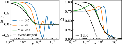
Figure 1: Particle $x_{\tau}$ in a harmonic trap displaced from $x=1$ to $x=0$ at time $0$. (a) The particle’s mean position $\langle x_{0}\rangle=1$ moves towards the new center of the trap, whereby oscillations occur for small damping. The probability density around $\langle x_{\tau}\rangle$ in this example is a Gaussian of constant width (see [49] for details and parameters). (b) Quality factor $Q$ of the transport bound for the simplest observable $z_{\tau}=x_{\tau}$, and quality factor of the TUR for the current $J_{t}=x_{t}-x_{0}$ in the overdamped case. Full saturation $Q=1$ at all times can be achieved for overdamped and underdamped dynamics as described below.

Example 1: Colloid in displaced trap.— Consider a bead trapped in a harmonic potential displaced from position $1$ to $0$ at time $\tau=0$. Knowing $\gamma$ and observing only the mean particle transport $\langle x_{t}-x_{0}\rangle$ we infer the entropy production from Eq. (1) to be $T\Delta S_{\rm tot}\geq T\Delta S_{\rm tot}^{\rm bound}\equiv\gamma\langle x_{t}-x_{0}\rangle^{2}/t$. We inspect the quality of the bound, $Q\equiv\Delta S_{\rm tot}^{\rm bound}/\Delta S_{\rm tot}\in[0,1]$, as a function of time (see Fig. 1). For underdamped dynamics $Q$ tends to $3/4$ at short times due to inertia (see for derivation). Using $z_{\tau}=x\nu(\tau)$ (for this example, $\nu$ turns out to be independent of $x,v$) we achieve saturation for all times, which is easily understood from our proof (see Appendix). Saturation for this example was also achieved via the transient correlation TUR [16]. However, the present approach is expected to be numerically more stable and requires less statistics, since a determination of fluctuations and derivatives of observables is not required. Moreover, the simplest version $z_{\tau}=x_{\tau}$ outperforms the transient TUR for the simplest current $J_{t}=x_{t}-x_{0}$ (dashed line in Fig. 1b). This may be interpreted as the magnitude of $x_{t}-x_{0}$ entering (1) being more relevant than its precision entering the TUR for this example. In contrast to the TUR [28], we also have the advantage that Eq. (1) holds for underdamped dynamics.

A disadvantage of Eq. (1) is that it is not useful for steady-state dynamics, since there $\langle z_{t}-z_{0}\rangle=0$. An exception are translation-invariant transients treated as non-equilibrium steady states (NESS) [50, 42]. A particular example are Brownian clocks [51] where for given $\Delta S_{\rm tot}$ the TUR limits precision whereas Eq. (1) limits the magnitude of transport, i.e., the size of the clock.

Example 2: Scattering experiments.—Since Eq. (1) only requires averages, it is applicable beyond single-molecule probes to bulk experiments, i.e., experiments on samples of many molecules probing mean properties, e.g., scattering techniques. The recent surge in the development of time-resolved X-ray scattering on proteins [34, 35, 36, 37, 52, 38, 39, 40, 41] renders our bound particularly useful. Here, transients may be excited by a pressure [53, 54] or temperature [55] quench, or one directly monitors slow kinetics [56]. One typically observes the structure factor $S(\mathbf{q})\equiv\frac{1}{N}\sum_{j,k=1}^{N}\langle\mathrm{e}^{-\mathrm{i}\mathbf{q}\cdot(\mathbf{r}_{t}^{\,j}-\mathbf{r}_{t}^{\,k})}\rangle$ [57, 58], where the sum runs over all scatterers (atoms, particles, etc.). This also applies to interacting colloid suspensions, where $S(\mathbf{q})$ is the Fourier transform of the pair correlation function [57]. An even simpler observable is the radius of gyration, $R_{g}^{2}\equiv\frac{1}{N}\sum_{j=1}^{N}\langle(\mathbf{r}_{j}-\bar{\mathbf{r}})^{2}\rangle$ [57, 59, 52], where $\bar{\mathbf{r}}\equiv\frac{1}{N}\sum_{j=1}^{N}\mathbf{r}_{j}$ is the center of mass. $R_{g}^{2}$ reflects the (statistical) size of molecules and is easily inferred from small $q$ via Guinier’s law, ${S(|\mathbf{q}|)\!\overset{|\mathbf{q}|\to 0}{=}\!S(0)\mathrm{e}^{-|\mathbf{q}|^{2}R_{g}^{2}/3}}$ [57, 59].

We consider the structure factor averaged over spatial dimensions $S(q)$ (see [49] for the vector version). For simplicity assume that $\gamma$ is a known scalar. We observe how $S(q)$ changes over time. From Eq. (1) we can derive the bounds (see [49])

$$T\Delta S_{\rm tot} \!\geq\!\frac{3\gamma[S_{t}(q)-S_{0}(q)]^{2}}{q^{2}\int_{0}^{t}[N-S_{\tau}(2q)]d\tau}\!\geq\!\frac{3\gamma[S_{t}(q)-S_{0}(q)]^{2}}{q^{2}t\max_{\tau}[N-S_{\tau}(2q)]}$$

$$T\Delta S_{\rm tot} \!\geq\!\frac{N[R_{g}^{2}(t)-R_{g}^{2}(0)]^{2}}{4\int_{0}^{t}d\tau R_{g}^{2}(\tau)/\gamma}\!\geq\!\frac{N[R_{g}^{2}(t)-R_{g}^{2}(0)]^{2}}{4t\max_{\tau}[R_{g}^{2}(\tau)]/\gamma}.$$ (6)

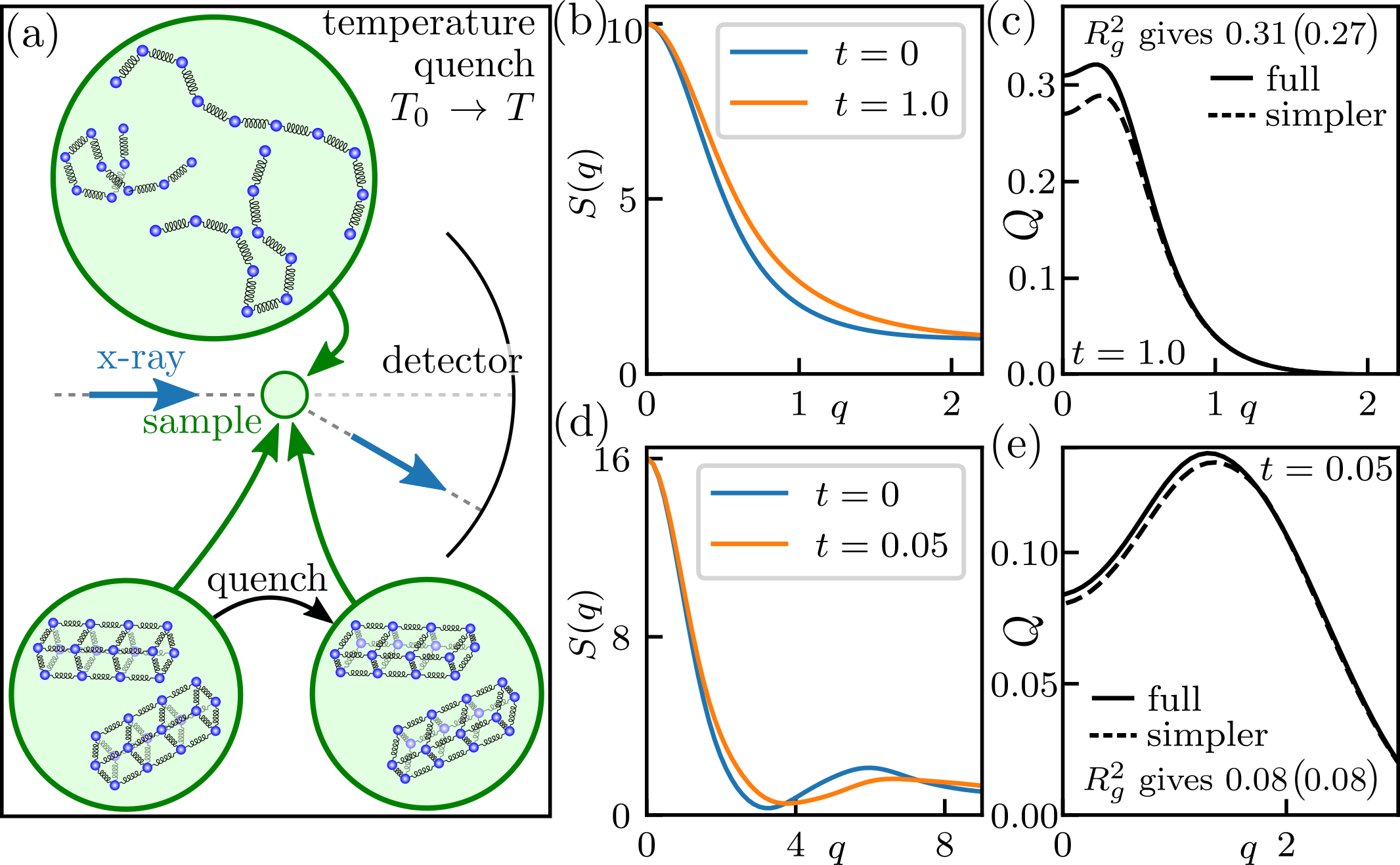
Figure 2: (a) Sketch of a scattering setup with (b,c) Rouse polymers with $N=10$ beads subject to a temperature quench from $T_{0}=2T$ to $T$ at $t=0$, and (d,e) harmonically confined “nano-crystal” with $N=16$ with Hookean neighbor-interactions subject to a quench in rest positions (see [49] for model details and parameters). (b,d) Structure factors and (c,e) corresponding quality factors [see Eq. (6); “simpler” bound contains $\max_{\tau}$ instead of integral].

The second bound in each line is a simplification when the maximum over time is known, and it is not necessary to measure for all $\tau$. The quality of these bounds for entropy production of internal degrees of freedom during relaxation is shown in Fig. 2 for a solution of (b,c) Rouse polymers upon a temperature quench (probing, e.g., the thermal relaxation asymmetry [60, 61, 62]) and (d,e) confined nano-crystals upon a structural transformation, respectively. Dissipative processes occur on distinct length scales, leading to changes of $S_{t}(q)$ at distinct $q$ (Fig. 2b,d). The sharpness of the bounds (6) depends on $q$, giving insight into the participation of distinct modes in dissipation. The $q$-dependence can in turn be used for optimization of inference. For small $q$ modes we recover the bound in terms of $R^{2}_{g}(\tau)$. We recover $\sim 30\;\%$ of $\Delta S_{\rm tot}$ in the quenched polymer solution and $\sim 15\;\%$ for the transforming nano-crystal. This is in fact a lot, since we only measure a 1d projection of $3(N-1)$ internal degrees of freedom.
The bound (1) will be useful for many bulk experiments beyond scattering. Consider, for example, a bulk measurement of the mean FRET efficiency for a pair of donor and acceptor chromophores with Förster distance $R_{0}$ attached to some macromolecule, $E_{t}=\langle(1+[(\mathbf{x}^{\rm don}_{t}-\mathbf{x}^{\rm acc}_{t})/R_{0}]^{6})^{-1}\rangle$, where the simplest bound reads $T\Delta S_{\rm tot}\geq R_{0}^{2}\gamma(E_{t}-E_{0})^{2}/8t$ (for details see [49]).

Example 3: Higher-order transport.— Consider now a centered transient process $x_{\tau}$, i.e., with constant mean $\langle x_{t}-x_{0}\rangle=0$. There is no mean transport. However, there is higher order transport, in the simplest case $\langle x_{t}^{2}-x_{0}^{2}\rangle\neq 0$. Setting $z_{\tau}=x_{\tau}^{2}$ we then have $T\Delta S_{\rm tot}\geq\gamma\langle x_{t}^{2}-x_{0}^{2}\rangle^{2}/4\int_{0}^{t}d\tau\langle x_{\tau}^{2}\rangle$. A concrete example are Brownian heat engines [63, 64, 65] in Fig. 3, where an “effective temperature” in a parabolic trap with stiffness $\kappa(\tau)$ is defined as $T_{\rm p}(\tau)\equiv\kappa(\tau)\langle x_{\tau}^{2}\rangle/k_{\rm B}$ [65].

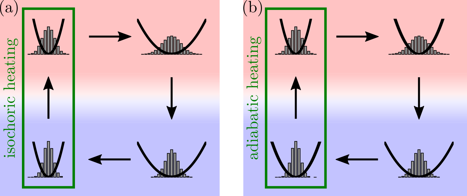
Figure 3: Schematic of (a) a Stirling heat engine as realized in Ref. [63] and (b) a Carnot heat engine with adiabatic heating and cooling [66] as realized in Ref. [64]. Note that the stiffness is constant (“isochoric”) during heating and cooling in (a) but not in (b). Red denotes hot and blue cold temperatures $T(\tau)$ of the environment (not to be confused with $T_{\rm p}$).

In this scenario, where the medium temperature varies in time, the LHS of the transport bound (1) becomes $T\Delta S_{\rm tot}\to\Delta(TS_{\rm tot})\equiv\int_{0}^{t}d\tau T(\tau)\dot{S}_{\rm tot}(\tau)$, yielding

$$\Delta(TS_{\rm tot})\geq\frac{\left[T_{\rm p}(t)-T_{\rm p}(0)-\int_{0}^{t}T_{\rm p}(\tau)\frac{\partial_{\tau}\kappa(\tau)}{\kappa(\tau)}d\tau\right]^{2}}{4\int_{0}^{t}T_{\rm p}(\tau)\kappa(\tau)d\tau/k_{\rm B}\gamma}.$$ (7)

During an isochoric heating step ($\kappa=\rm constant$ such that $\partial_{\tau}\kappa(\tau)=0$) highlighted in Fig. 3a, no work is performed [63], and the dissipation $\Delta(TS_{\rm tot})$ of an efficient engine should be minimal. Thus, to achieve a given $T_{\rm p}(t)-T_{\rm p}(0)$ for minimal $\Delta(TS_{\rm tot})$, we either need long $t$ or must maximize $\int_{0}^{t}d\tau T_{\rm part}(\tau)$, implying substantial heating at the beginning of the time interval $[0,t]$. For time-dependent $\kappa(\tau)$ (see Fig. 3b or the Carnot engine [64]), the bound in Eq. (7) is more complicated since all terms contribute when $\partial_{\tau}\kappa(\tau)\neq 0$. However, the bound still serves as a fundamental limit that can be evaluated for any given protocol. Note that the results equally apply to underdamped heat engines (as theoretically considered in, e.g., [69]).

An insightful observable is the characteristic function $\phi_{\tau}(\mathbf{q})\equiv\langle{\rm e}^{-\mathbf{q}\cdot\mathbf{x}_{\tau}}\rangle$ encoding information on moments of all order. The transport bound for $\phi_{\tau}(\mathbf{q})$ reads

$$T\Delta S_{\rm tot}\geq\frac{[\phi_{t}(\mathbf{q})-\phi_{0}(\mathbf{q})]^{2}}{\int_{0}^{t}d\tau\phi_{\tau}(2\mathbf{q})\mathbf{q}^{T}\bm{\gamma}^{-1}(\tau)\mathbf{q}}\,,$$ (8)

and quantifies how changes of the $q$-th mode of the probability density contribute to $\Delta S_{\rm tot}$. Eq. (8) will be useful for proving other bounds.

Interpretation and handling of $\mathcal{D}^{z}(t)$.—The interpretation of $\mathcal{D}^{z}(t)$ is intuitive: for a process $\mathbf{x}_{\tau}$ with given cost $\Delta S_{\rm tot}$, the transport $\langle z_{t}-z_{0}\rangle$ will be larger for a function $z$ that stretches $\mathbf{x}$ more. This stretching is re-scaled by $\nabla_{\mathbf{x}}z$ in the quadratic form $\mathcal{D}^{z}(t)$.

For simple marginal observations, $z(\mathbf{x})=x_{i}$, we have that $\mathcal{D}^{z}={\bm{\gamma}^{-1}}_{ii}$. Moreover, if we only observe $z_{\tau}$ but not $\mathbf{x}_{\tau}$, we can often bound $\mathcal{D}^{z}(t)$ in terms of $\langle z_{\tau}\rangle$ or in terms of constants, such as in the case of $R_{g}^{2}$ and $S_{t}(q)$ before (e.g., it suffices to know that $z_{\tau}$ has bounded derivatives). In the challenging case where we only observe $z_{\tau}$ but do not know the function $z(\mathbf{x})$ (i.e., it is some unknown projection or reaction coordinate), we can, given sufficient time resolution, determine or estimate $\mathcal{D}^{z}$ as follows: For overdamped dynamics we have $t\mathcal{D}^{z}(t)=\int_{0}^{t}d\tau\frac{{\rm var}[dz_{\tau}]}{2k_{\rm B}Td\tau}$ (for steady-state dynamics see [70], where $\mathcal{D}^{z}$ recently appeared in a correlation inequality). For underdamped dynamics, scalar $m,\gamma$, and $z_{\tau}=z(\mathbf{x}_{\tau})$ (no explicit time dependence) we can obtain $\mathcal{D}^{z}(t)$ if we know the momentum relaxation time $m/\gamma$ via $\frac{{\rm var}\left(d\left[\frac{d}{d\tau}z(\mathbf{x}_{\tau})\right]\right)}{2k_{\rm B}Tdt}=\frac{\gamma^{2}}{m^{2}}\langle\gamma^{-1}[\nabla_{\mathbf{x}}z(\mathbf{x}_{\tau})]^{2}\rangle$. If the system relaxes to equilibrium we can obtain $\gamma/m$ from observations of $z_{\tau}$ via equilibrium measurements of ${\rm var}(d[\frac{d}{d\tau}z(\mathbf{x}_{\tau})])$ and ${\rm var}(dz(\mathbf{x}_{\tau}))$ (see [49]). If the system relaxes to a NESS, we can upper bound $\mathcal{D}^{z}$ by using that $m/\gamma\leq t_{\rm rel}$ with the relaxation time of the system determined, e.g. from correlation functions $t^{-1}_{\rm rel}=-\lim_{t\to\infty}t^{-1}\ln[\langle z_{t}z_{0}\rangle-\langle z_{t}\rangle\langle z_{0}\rangle]$ (see [49]).

Conclusion.—We proved an inequality upper-bounding transport of any scalar observable in a general $d$-dimensional non-equilibrium system in terms of the total entropy production and fluctuation-scale function that “corrects” for the amount the observation stretches microscopic coordinates. We explained how to saturate the bound. The result, classifiable as a time-integrated generalized speed limit, may be understood as a thermodynamic cost of transport of observables and allows for inferring a lower bound on dissipation, thus complementing the TUR and existing speed limits. The bound places underdamped and overdamped stochastic as well as deterministic systems on equal footing. This fills an important gap, because microscopic dynamics is—at least on short time scales—underdamped, and the TUR does not hold for underdamped dynamics. In particular short-time TURs for overdamped dynamics [8, 9, 71] are expected to fail.

By only requiring averages, the transport bound is statistically less demanding and applicable to both, single-molecule as well as bulk experiments. This is attractive in the context of time-resolved X-ray scattering on biomolecules, as it will allow thermodynamic inference from bulk observations of controlled transients [53, 54, 55, 56]. This may facilitate thermodynamic inference on molecular machines without an obvious directionality such molecular chaperones [32], which remains challenging even with most advanced single-molecule techniques [33]. The bound allows for versatile applications and generalizations to vectorial observables $\mathbf{z}$ and adaptations for Markov-jump dynamics.

Acknowledgments.—Financial support from the European Research Council (ERC) under the European Union’s Horizon Europe research and innovation program (grant agreement No 101086182 to AG) is gratefully acknowledged.

Appendix: Sketch of proof.— To prove Eq. (1) we use the Cauchy-Schwarz inequality for stochastic integrals similarly as in [16] but generalized to underdamped dynamics (detailed proof in [49]). We define the stochastic integrals $A_{t}\equiv\int_{\tau=0}^{\tau=t}{\bm{\nu}}(\mathbf{x}_{\tau},\mathbf{v}_{\tau},\tau)\cdot\sqrt{\bm{\gamma}}d\mathbf{W}_{\tau}$ and $B_{t}\equiv\int_{\tau=0}^{\tau=t}\{\nabla_{\mathbf{x}}z_{\tau}\}\cdot{\sqrt{\bm{\gamma}}^{-1}}^{T}d\mathbf{W}_{\tau}$ for which we can show that $\langle A_{t}^{2}\rangle=T\Delta S_{\rm tot}$ and $\langle B_{t}^{2}\rangle=t\mathcal{D}^{z}(t)$. The Cauchy-Schwarz inequality thus implies $T\Delta S_{\rm tot}\geq\langle A_{t}B_{t}\rangle^{2}/t\mathcal{D}^{z}(t)$. To complete the proof, we compute $\langle A_{t}B_{t}\rangle=\langle\int_{0}^{t}{\bm{\nu}}(\mathbf{x}_{\tau},\mathbf{v}_{\tau},\tau)\cdot\left\{\nabla_{\mathbf{x}}z_{\tau}\right\}d\tau\rangle$ via rewriting $\{\nabla_{\mathbf{x}}z_{\tau}\}=\bm{\gamma}\mathbf{m}^{-1}\nabla_{\mathbf{v}}\{\nabla_{\mathbf{v}}^{T}\mathbf{m}\bm{\gamma}^{-1}\nabla_{\mathbf{x}}z_{\tau}\}$, integrating by parts in $\nabla_{\mathbf{v}}$, and substituting the Klein-Kramers equation in the form $\nabla_{\mathbf{v}}\cdot\mathbf{m}^{-1}\bm{\gamma}{\bm{\nu}}\rho=[\nabla_{\mathbf{x}}\cdot\mathbf{v}+\nabla_{\mathbf{v}}\cdot\mathbf{m}^{-1}\mathbf{F}(\mathbf{x},\tau)+\partial_{\tau}]\rho(\mathbf{x},\mathbf{v},\tau)$, which upon further integrations by parts and simplifications yields $\langle A_{t}B_{t}\rangle=\int_{0}^{t}d\tau\left\langle\mathbf{v}_{\tau}\cdot\nabla_{\mathbf{x}}z_{\tau}\right\rangle=\langle\int_{0}^{t}d\tau(\frac{d}{d\tau}-\partial_{\tau})z_{\tau}\rangle=\langle z_{t}-z_{0}-\int_{0}^{t}\partial_{\tau}z_{\tau}d\tau\rangle$.

From the proof we immediately know how to achieve saturation by saturating the Cauchy-Schwarz inequality, allowing optimal inference. Saturation occurs for $\nabla_{\mathbf{x}}z_{\tau}=c\bm{\gamma}{\bm{\nu}}(\mathbf{x},\mathbf{v},\tau)$ for any constant $c$. While one may not always be able to choose $z$ this way, one should aim to approach this for saturation. If $d=1$ (with natural boundaries) and ${\bm{\nu}}$ does not depend on $\mathbf{v}$, saturation is always feasible.

In this Supplemental Material we provide derivations and additional details for results and examples shown in the Letter. We provide the detailed derivation of the main result, and details and parameters complementing the examples in Figs. 1 and 2. Moreover, we explain in detail how to obtain $\mathcal{D}^{z}$ from short-time fluctuations.

I Proof of the main result

Here, we prove our main result, i.e., the transport bound in Eq. (1) in the Letter. Consider underdamped stochastic dynamics as in Eq. (2) in the Letter. Consider positive definite symmetric matrices $\mathbf{m}$ and $\bm{\gamma}(\tau)$ (for simplicity denote the latter by $\bm{\gamma}$). Using the “local mean velocity” ${\bm{\nu}}$ as in Eq. (4) in the Letter we can write the underdamped Klein-Kramers dynamics as [1]

$${\bm{\nu}}(\mathbf{x},\mathbf{v},\tau) \equiv\mathbf{v}_{\tau}+k_{\rm B}T\mathbf{m}^{-1}\frac{\nabla_{\mathbf{v}}\rho(\mathbf{x},\mathbf{v},t)}{\rho(\mathbf{x},\mathbf{v},t)}$$

$$\partial_{\tau}\rho(\mathbf{x},\mathbf{v},t) =\left(-\nabla_{\mathbf{x}}\cdot\mathbf{v}+\mathbf{m}^{-1}\nabla_{\mathbf{v}}\cdot\left[-\mathbf{F}(\mathbf{x},\tau)+{\bm{\gamma}(\tau){\bm{\nu}}(\mathbf{x},\mathbf{v},\tau)}\right]\right)\rho(\mathbf{x},\mathbf{v},t)\,.$$ (S1)

Recalling the setup of the proof as presented in the Appendix, and using the white noise property/Wiener correlation $\langle{\rm d}W_{\tau}^{i}{\rm d}W_{\tau^{\prime}}^{j}\rangle=\delta(\tau-\tau^{\prime}){\rm d}\tau{\rm d}\tau^{\prime}$ we have

$$A_{t} \equiv\int_{\tau=0}^{\tau=t}{\bm{\nu}}(\mathbf{x}_{\tau},\mathbf{v}_{\tau},\tau)\cdot\sqrt{\bm{\gamma}}{\rm d}\mathbf{W}_{\tau}$$

$$B_{t} \equiv\int_{\tau=0}^{\tau=t}\left\{\nabla_{\mathbf{x}}z(\mathbf{x}_{\tau},\tau)\right\}\cdot{\sqrt{\bm{\gamma}}^{-1}}^{T}{\rm d}\mathbf{W}_{\tau}$$

$$\langle A_{t}^{2}\rangle =\int_{0}^{t}{\rm d}\tau\langle{\bm{\nu}}^{T}(\mathbf{x}_{\tau},\mathbf{v}_{\tau},\tau)\bm{\gamma}{\bm{\nu}}(\mathbf{x}_{\tau},\mathbf{v}_{\tau},\tau)\rangle=T\Delta S_{\rm tot}([0,t])$$

$$\langle B_{t}^{2}\rangle =\int_{0}^{t}{\rm d}\tau\left\langle\left\{\nabla_{\mathbf{x}}z(\mathbf{x}_{\tau},\tau)\right\}^{T}\bm{\gamma}^{-1}\left\{\nabla_{\mathbf{x}}z(\mathbf{x}_{\tau},\tau)\right\}\right\rangle\equiv t\mathcal{D}^{z}(t)\,.$$ (S2)

Using the Einstein summation convention, we can check the matrix differential operator identity for a constant (i.e. $\mathbf{x}$-independent) invertible $d\times d$ matrix $\mathbf{G}$

$$(\mathbf{G}\nabla_{\mathbf{v}})[\mathbf{v}\cdot\mathbf{G}^{-1}\nabla_{\mathbf{x}}z(\mathbf{x},\tau)]=\mathbf{e}_{i}G_{ij}\partial_{v_{j}}v_{n}(\mathbf{G}^{-1})_{nm}\partial_{x_{m}}z(\mathbf{x},\tau)=\mathbf{e}_{i}G_{in}(\mathbf{G}^{-1})_{nm}\partial_{x_{m}}z(\mathbf{x},\tau)=\nabla_{\mathbf{x}}z(\mathbf{x},\tau)\,.$$ (S3)

Using this identity for the choice $\mathbf{G}^{-1}=\mathbf{m}\bm{\gamma}^{-1}$, integrating by parts, and substituting Eq. (S1) for $\nabla_{\mathbf{v}}\cdot\mathbf{m}^{-1}\bm{\gamma}{\bm{\nu}}$, we obtain

$$-\langle A_{t}B_{t}\rangle =-\int_{0}^{t}{\rm d}\tau\int{\rm d}\mathbf{x}\int{\rm d}\mathbf{v}\left\{\mathbf{G}\nabla_{\mathbf{v}}[\mathbf{v}\cdot\mathbf{G}^{-1}\nabla_{\mathbf{x}}z(\mathbf{x},\tau)]\right\}\cdot{\bm{\nu}}(\mathbf{x},\mathbf{v},\tau)\rho(\mathbf{x},\mathbf{v},\tau)$$

$$=\int_{0}^{t}{\rm d}(\mathbf{x},\mathbf{v},\tau)\{\mathbf{v}\cdot\mathbf{G}^{-1}\nabla_{\mathbf{x}}z(\mathbf{x},\tau)\}\nabla_{\mathbf{v}}\cdot\mathbf{G}^{T}{\bm{\nu}}(\mathbf{x},\mathbf{v},\tau)\rho(\mathbf{x},\mathbf{v},\tau)$$

$$=\int_{0}^{t}{\rm d}(\mathbf{x},\mathbf{v},\tau)\{\mathbf{v}\cdot\mathbf{G}^{-1}\nabla_{\mathbf{x}}z(\mathbf{x},\tau)\}\mathbf{m}^{-1}\nabla_{\mathbf{v}}\cdot\bm{\gamma}{\bm{\nu}}(\mathbf{x},\mathbf{v},\tau)\rho(\mathbf{x},\mathbf{v},\tau)$$

$$=\int_{0}^{t}{\rm d}\tau\int{\rm d}\mathbf{x}\int{\rm d}\mathbf{v}\{\mathbf{v}\cdot\mathbf{G}^{-1}\nabla_{\mathbf{x}}z(\mathbf{x},\tau)\}\left[\nabla_{\mathbf{x}}\cdot\mathbf{v}+\mathbf{m}^{-1}\nabla_{\mathbf{v}}\cdot\mathbf{F}(\mathbf{x},\tau)+\partial_{\tau}\right]\rho(\mathbf{x},\mathbf{v},\tau)$$

$$=\left\langle\mathbf{v}_{t}\cdot\mathbf{G}^{-1}\nabla_{\mathbf{x}}z(\mathbf{x}_{t},t)-\mathbf{v}_{0}\cdot\mathbf{G}^{-1}\nabla_{\mathbf{x}}z(\mathbf{x}_{0},0)\right\rangle$$

$$\quad-m\int_{0}^{t}{\rm d}\tau\left\langle(\mathbf{v}_{\tau}\cdot\nabla_{\mathbf{x}})[\mathbf{v}_{\tau}\cdot\mathbf{G}^{-1}\nabla_{\mathbf{x}}z(\mathbf{x}_{\tau},\tau)]+\frac{\mathbf{F}(\mathbf{x}_{\tau},\tau))}{m}\cdot\mathbf{G}^{-1}\nabla_{\mathbf{x}}z(\mathbf{x}_{\tau},\tau)+\mathbf{v}_{\tau}\cdot\mathbf{G}^{-1}\nabla_{\mathbf{x}}\dot{z}(\mathbf{x}_{\tau},\tau)\right\rangle\,.$$ (S4)

Note that

$$\left\langle\mathbf{v}_{t}\cdot\mathbf{G}^{-1}\nabla_{\mathbf{x}}z(\mathbf{x}_{t},t)-\mathbf{v}_{0}\cdot\mathbf{G}^{-1}\nabla_{\mathbf{x}}z(\mathbf{x}_{0},0)\right\rangle=\left\langle\int_{0}^{t}{\rm d}\tau\frac{{\rm d}}{{\rm d}\tau}[\mathbf{v}_{\tau}\cdot\mathbf{G}^{-1}\nabla_{\mathbf{x}}z(\mathbf{x}_{\tau},\tau)]\right\rangle\,,$$ (S5)

and use the equation of motion in Eq. (S1) to see that

$$\left\langle\frac{{\rm d}}{{\rm d}\tau}[\mathbf{v}_{\tau}\cdot\mathbf{G}^{-1}\nabla_{\mathbf{x}}z(\mathbf{x}_{\tau},\tau)]\right\rangle =\left\langle\frac{\mathbf{F}(\mathbf{x}_{\tau},\tau)-\bm{\gamma}\mathbf{v}_{\tau}}{m}\cdot\mathbf{G}^{-1}\nabla_{\mathbf{x}}z(\mathbf{x}_{\tau},\tau)+\mathbf{v}_{\tau}\cdot\mathbf{G}^{-1}\nabla_{\mathbf{x}}[\mathbf{v}_{\tau}\cdot\nabla_{\mathbf{x}}z(\mathbf{x}_{\tau},\tau)+\dot{z}(\mathbf{x}_{\tau},\tau)]\right\rangle\,.$$ (S6)

Since $\mathbf{G}$ is independent of $\mathbf{x}$ we have

$$(\mathbf{v}_{\tau}\cdot\nabla_{\mathbf{x}})[\mathbf{v}_{\tau}\cdot\mathbf{G}^{-1}\nabla_{\mathbf{x}}z(\mathbf{x}_{\tau},\tau)]=(\mathbf{v}_{\tau}\cdot\mathbf{G}^{-1}\nabla_{\mathbf{x}})[\mathbf{v}_{\tau}\cdot\nabla_{\mathbf{x}}z(\mathbf{x}_{\tau},\tau)]\,,$$ (S7)

which allows to conclude that

$$-\langle A_{t}B_{t}\rangle =-\int_{0}^{t}{\rm d}\tau\left\langle\mathbf{v}_{\tau}\cdot\nabla_{\mathbf{x}}z(\mathbf{x}_{\tau},\tau)\right\rangle\,.$$ (S8)

Moreover, using

$$\frac{{\rm d}}{{\rm d}\tau}z(\mathbf{x}_{\tau},\tau)=\mathbf{v}_{\tau}\cdot\nabla_{\mathbf{x}}z(\mathbf{x}_{\tau},\tau)+\partial_{\tau}z(\mathbf{x}_{\tau},\tau)\,,$$ (S9)

we obtain

$$\langle A_{t}B_{t}\rangle =\left\langle z(\mathbf{x}_{t},t)-z(\mathbf{x}_{0},0)-\int_{0}^{t}{\rm d}\tau\partial_{\tau}z(\mathbf{x}_{\tau},\tau)\right\rangle\,.$$ (S10)

With Eq. (S2) this proves via Cauchy-Schwarz $\langle A_{t}B_{t}\rangle^{2}\leq\langle A_{t}^{2}\rangle\langle B_{t}^{2}\rangle$ the transport bound

$$\frac{\left\langle z(\mathbf{x}_{t},t)-z(\mathbf{x}_{0},0)-\int_{0}^{t}{\rm d}\tau\partial_{\tau}z(\mathbf{x}_{\tau},\tau)\right\rangle^{2}}{t\mathcal{D}^{z}(t)/k_{\rm B}T}\leq T\Delta S_{\rm tot}\,.$$ (S11)

I.1 Overdamped limit

Although the underdamped results already contain the overdamped and Newtonian cases as limiting results, it is interesting to see that the derivation in the overdamped case greatly simplifies. Here, we have that $\nabla_{\mathbf{x}}\cdot{\bm{\nu}}(\mathbf{x},\tau)\rho(\mathbf{x},\tau)=-\partial_{\tau}\rho(\mathbf{x},\tau)$ [1] such that Eq. (S11) directly follows from

$$\langle A_{t}B_{t}\rangle =\int_{0}^{t}{\rm d}\tau\int{\rm d}\mathbf{x}\left\{\nabla_{\mathbf{x}}z(\mathbf{x},\tau)]\right\}\cdot{\bm{\nu}}(\mathbf{x},\tau)\rho(\mathbf{x},\tau)$$

$$=\int_{0}^{t}{\rm d}\tau\int{\rm d}\mathbf{x}z(\mathbf{x},\tau)\partial_{\tau}\rho(\mathbf{x},\tau)$$

$$=\left\langle z(\mathbf{x}_{t},t)-z(\mathbf{x}_{0},0)-\int_{0}^{t}{\rm d}\tau\partial_{\tau}z(\mathbf{x}_{\tau},\tau)\right\rangle\,.$$ (S12)

II Details on the example in Fig. 1 in the Letter

Here, we give details on the example of the displaced trap considered in Fig. 1 in the Letter. Note that the overdamped case of this example including application of the TUR can be found in [2]. In Figure 1 we consider the parameters $a=5$, $m=1$ and $y=1$. In the overdamped case, $\gamma$ cancels out in the quality factor.

The underdamped equations of motion for this example for a linear force originating from a harmonic potential around $0$ with a stiffness $a$ read

$${\rm d}\begin{bmatrix}x_{\tau}\\ v_{\tau}\end{bmatrix} =-\underbrace{\begin{bmatrix}0&-1\\ a\frac{\gamma}{m}&\frac{\gamma}{m}\end{bmatrix}}_{\equiv\mathbf{A}}\begin{bmatrix}x_{\tau}\\ v_{\tau}\end{bmatrix}{\rm d}\tau+\underbrace{\frac{\sqrt{2k_{\rm B}T\gamma}}{m}\begin{bmatrix}0&0\\ 0&1\end{bmatrix}}_{\equiv\bm{\sigma}}{\rm d}\mathbf{W}_{\tau}$$

$$\mathbf{D} =\frac{\bm{\sigma}\bm{\sigma}^{T}}{2}=\frac{k_{\rm B}T\gamma}{m^{2}}\begin{bmatrix}0&0\\ 0&1\end{bmatrix}\,.$$ (S13)

The steady-state covariance matrix $\bm{\Sigma}_{\rm s}$ and time-dependent covariance $\bm{\Sigma}(t)$ obey the Lyapunov equations (see, e.g., Supplemental Material of Ref. [3] for a short derivation)

$$\mathbf{A}\bm{\Sigma}_{\rm s}+\bm{\Sigma}_{\rm s}\mathbf{A}^{T} =2\mathbf{D}=\bm{\sigma}\bm{\sigma}^{T}$$

$$\bm{\Sigma}(t) =\bm{\Sigma}_{\rm s}+\mathrm{e}^{-\mathbf{A}t}[\bm{\Sigma}(0)-\bm{\Sigma}_{\rm s}]\mathrm{e}^{-\mathbf{A}^{T}t}\,.$$ (S14)

We assume the particle to be equilibrated in the trap around $\langle x_{0}\rangle=y$ before displacing the trap at time $t=0$ to position $x=0$. Therefore we have

$$\bm{\Sigma}(0)=\bm{\Sigma}_{\rm s} =k_{\rm B}T\begin{bmatrix}\frac{1}{a\gamma}&0\\ 0&\frac{1}{m}\end{bmatrix}\,,$$ (S15)

which can be also obtained from equipartition.

We see from Eq. (S14) that $\bm{\Sigma}(\tau)=\bm{\Sigma}_{\rm s}$ for all $\tau\geq 0$, i.e., the covariance remains unchanged, and in particular there will be no coupling of positions and velocities, and the density reads

$$\rho(x,v,\tau)=\frac{\sqrt{a\gamma m}}{2\pi}\exp\left[-\frac{a\gamma(x-\langle x_{\tau}\rangle)^{2}+m(v-\langle v_{\tau}\rangle)^{2}}{2k_{\rm B}T}\right]\,.$$ (S16)

The mean starting from $\langle x_{0}\rangle=y$ and $\langle v_{0}\rangle=0$ is governed by

$$\begin{bmatrix}\langle x_{\tau}\rangle\\ \langle v_{\tau}\rangle\end{bmatrix}=\exp(-\mathbf{A}\tau)\begin{bmatrix}y\\ 0\end{bmatrix}\,.$$ (S17)

The decisive term for the entropy production is [see Eqs. (4) and (5) in the Letter]

$$T\Delta S_{\rm tot} =\gamma\int_{0}^{t}{\rm d}\tau\left\langle\left[v_{\tau}+\frac{k_{\rm B}T}{m}\,\frac{\partial_{v}\rho(x_{\tau},v_{\tau},\tau)}{\rho(x_{\tau},v_{\tau},\tau)}\right]^{2}\right\rangle$$

$$=\gamma\int_{0}^{t}{\rm d}\tau\left\langle\left[v_{\tau}-\frac{k_{\rm B}T}{m}\,\frac{2m(v_{\tau}-\langle v_{\tau}\rangle)}{2k_{\rm B}T}\right]^{2}\right\rangle$$

$$=\gamma\int_{0}^{t}{\rm d}\tau\left\langle v_{\tau}\right\rangle^{2}\,.$$ (S18)

Note that in this simple example, the local mean velocity is not local, i.e., it does not depend on $x_{\tau}$. In the overdamped case we have $\nu(\tau)=-az\mathrm{e}^{-a\tau}$ (see Supplemental Material of Ref. [2]), but in the underdamped case the eigenvalues of $\mathbf{A}$ can become complex (signaling oscillations)

$$\mathbf{A} =\begin{bmatrix}0&-1\\ a\frac{\gamma}{m}&\frac{\gamma}{m}\end{bmatrix}$$

$$0 =\lambda^{2}-\frac{\gamma}{m}\lambda+a\frac{\gamma}{m}$$

$$\lambda_{1,2} =\frac{\gamma}{2m}\left[1\pm\sqrt{1-\frac{4am}{\gamma}}\,\right]\,.$$ (S19)

We obtain oscillations for $4am>\gamma$, i.e., for weak damping.

II.1 Saturation

We know from the Cauchy-Schwarz proof of Eq. (S11) that we obtain saturation for $\gamma\nu(x,v,\tau)=c\partial_{x}z(x,\tau)$, i.e., in this case the optimal observable $z_{\rm opt}$ is given by

$$\gamma\nu(x,v,\tau) =\gamma\nu(\tau)\overset{\rm as\ in\ Eq.~{}\eqref{displaced trap entropy}}{=}\gamma\langle v_{\tau}\rangle\equiv\gamma f(\tau)$$

$$z_{\rm opt}(x,\tau) =\gamma x\langle v_{\tau}\rangle=\gamma x\underbrace{\left(\begin{bmatrix}0\\ 1\end{bmatrix}\cdot\exp(-\mathbf{A}\tau)\begin{bmatrix}y\\ 0\end{bmatrix}\right)}_{=f(\tau)}.$$ (S20)

Since the Cauchy-Schwarz inequality becomes saturated for this choice, we know that the transport bound Eq. (S11) is saturated, allowing optimal inference of $\Delta S_{\rm tot}$.

This predicted saturation can be checked for this case by computing

$$T\Delta S_{\rm tot} =\gamma\int_{0}^{t}{\rm d}\tau f^{2}(\tau)$$

$$t\mathcal{D}^{z_{\rm opt}}(t) =\gamma\int_{0}^{t}{\rm d}\tau f^{2}(\tau)=T\Delta S_{\rm tot}$$

$$\left\langle z_{\rm opt}(\mathbf{x}_{t},t)-z_{\rm opt}(\mathbf{x}_{0},0)-\int_{0}^{t}{\rm d}\tau\partial_{\tau}z_{\rm opt}(\mathbf{x}_{\tau},\tau)\right\rangle =\gamma\langle x_{t}\rangle f(t)-\gamma\langle x_{0}\rangle\underbrace{f(0)}_{=0}-\gamma\int_{0}^{t}{\rm d}\tau\langle x_{\tau}\rangle\partial_{\tau}f(\tau)=$$

$$=\gamma\int_{0}^{t}{\rm d}\tau f(\tau)\partial_{\tau}\langle x_{\tau}\rangle=\gamma\int_{0}^{t}{\rm d}\tau f^{2}(\tau)=T\Delta S_{\rm tot}\,.$$ (S21)

Hence we indeed have saturation since the transport bound (S11) here reads $\Delta S_{\rm tot}^{2}/\Delta S_{\rm tot}\overset{\rm here\ =}{\leq}\Delta S_{\rm tot}$.

II.2 Short-time limit

In Fig. 1b we see that the short-time limit of the quality factor is $3/4$. This can be confirmed analytically as follows,

$$\begin{bmatrix}\langle x_{\tau}\rangle\\ \langle v_{\tau}\rangle\end{bmatrix}=\exp(-\mathbf{A}\tau)\begin{bmatrix}y\\ 0\end{bmatrix}=\begin{bmatrix}y\\ 0\end{bmatrix}-\tau\begin{bmatrix}0&-1\\ a\frac{\gamma}{m}&\frac{\gamma}{m}\end{bmatrix}\begin{bmatrix}y\\ 0\end{bmatrix}+\mathcal{O}(\tau^{2})=\begin{bmatrix}y\\ -\frac{\tau az\gamma}{m}\end{bmatrix}+\frac{\tau^{2}}{2}\left[\begin{matrix}-\frac{\gamma ay}{m}\\ \frac{\gamma^{2}ay}{m^{2}}\end{matrix}\right]+\mathcal{O}(\tau^{3})\,.$$ (S22)

Thus, the short-time entropy production reads

$$T\Delta S_{\rm tot} =\frac{\gamma^{3}t^{3}a^{2}y^{2}}{3m^{2}}+\mathcal{O}(t^{4})\,.$$ (S23)

The short-time transport reads

bound $$=\frac{\gamma}{t}(\langle x_{t}\rangle-y)^{2}=\frac{\gamma}{t}\frac{t^{4}}{4}\frac{\gamma^{2}a^{2}y^{2}}{m^{2}}+\mathcal{O}(t^{4})=\frac{3}{4}T\Delta S_{\rm tot}+\mathcal{O}(t^{4})\,,$$ (S24)

such that the short-time quality factor is indeed $3/4$.

III Derivation of Eq. (6) in the Letter

Here, we apply and rearrange the transport bound for the radius of gyration and structure factor, reproducing the bounds presented in Eq. (6) in the Letter.

III.1 Radius of gyration

First, to approach the radius of gyration consider the following observable $z$, which yields $NR_{g}^{2}=\langle z_{\tau}\rangle$,

$$\vec{c} \equiv\frac{1}{N}\sum_{k=1}^{N}\vec{x}_{k}$$

$$z(\mathbf{x}) \equiv\sum_{j=1}^{N}(\vec{x}_{j}-\vec{c}\,)^{2}$$

$$NR_{g}^{2}(t) =\langle z(\mathbf{x}_{t})\rangle\,,$$ (S25)

where the $\vec{x}_{j}$ are the 3d position vectors of the individual beads. Here, we denote 3d vectors by arrows and boldface notation is only used for the $3N$ dimensional vectors that contain all bead positions.

To compute $\mathcal{D}^{z}$ we need to compute derivatives, i.e., compute

$$\vec{\nabla}_{l}z(\mathbf{x}) =2(\vec{x}_{l}-\vec{c})-\frac{2}{N}\sum_{j=1}^{N}(\vec{x}_{j}-\vec{c})\,.$$ (S26)

For the full $3N$-dimensional gradient we obtain

$$\frac{[\nabla z(\mathbf{x})]^{2}}{4} =z(\mathbf{x})-\frac{1}{N}\sum_{j,l=1}^{N}(\vec{x}_{j}-\vec{c})\cdot(\vec{x}_{l}-\vec{c})$$

$$=z(\mathbf{x})-\frac{1}{N}\left[\sum_{j=1}^{N}(\vec{x}_{j}-\vec{c})\right]^{2}$$

$$=z(\mathbf{x})\,.$$ (S27)

This yields the transport bound for $R_{g}^{2}$ in Eq. (6) in the Letter. To further generalize, note that for time-dependent $\gamma(\tau)$, the factor $1/\gamma$ has to be kept inside the time integral. Moreover, note that if the beads have different $\gamma_{j}$ we may formulate the bound in terms of the minimum of these $\gamma_{j}$.

III.2 Structure factor

Consider the following $z_{\tau}$ and its derivative to approach $S_{t}(\vec{q})$ and the corresponding $\mathcal{D}^{z}(t)$,

$$z(\mathbf{x}) \equiv\frac{1}{N}\sum_{j,k=1}^{N}\cos[\vec{q}\cdot(\vec{x}_{j}-\vec{x}_{k})]$$

$$S_{t}(\vec{q}) =\langle z(\mathbf{x}_{t})\rangle$$

$$\vec{\nabla}_{j}z(\mathbf{x}) =-\frac{2\vec{q}}{N}\sum_{k=1}^{N}\sin[\vec{q}\cdot(\vec{x}_{j}-\vec{x}_{k})]$$

$$A_{N} \equiv\frac{N^{2}}{4\vec{q}^{\,2}}[\nabla z(\mathbf{x})]^{2}=\sum_{j,k,l=1}^{N}\sin[\vec{q}\cdot(\vec{x}_{j}-\vec{x}_{k})]\sin[\vec{q}\cdot(\vec{x}_{j}-\vec{x}_{l})]\,.$$ (S28)

In order to express the derivative in observable terms, consider the expression

$$B_{N} \equiv\frac{N^{2}-Nz_{2\vec{q}}(\mathbf{x})}{4}=\frac{1}{4}\sum_{k,l=1}^{N}\left(1-\cos[2\vec{q}\cdot(\vec{x}_{k}-\vec{x}_{l})]\right)=\frac{1}{2}\sum_{j,k=1}^{N}\sin^{2}[\vec{q}\cdot(\vec{x}_{k}-\vec{x}_{l})]\,.$$ (S29)

Introduce the notation $s_{jk}=-s_{kj}=\sin[\vec{q}\cdot(\vec{x}_{j}-\vec{x}_{k})]$ and note that from relabeling indices we get

$$6(NB_{N}-A_{N}) =3N\sum_{k,l=1}^{N}s_{kl}^{2}-6\sum_{j,k,l=1}^{N}s_{jl}s_{jk}$$

$$=\sum_{j,k,l=1}^{N}\left(s_{jl}^{2}+s_{lk}^{2}+s_{kj}^{2}+2s_{jl}s_{lk}+2s_{lk}s_{kj}+2s_{kj}s_{jl}\right)$$

$$=\sum_{j,k,l=1}^{N}(s_{jl}+s_{lk}+s_{kj})^{2}$$

$$\geq 0\,,$$ (S30)

with equality for $q\to 0$. This implies an upper bound of $t\mathcal{D}^{z}=4\vec{q}^{\,2}\int_{0}^{t}{\rm d}\tau\langle A_{N}(\tau)\rangle/N^{2}\leq 4\vec{q}^{\,2}\int_{0}^{t}{\rm d}\tau\langle B_{N}(\tau)\rangle/N$ that implies the vector-version of the bound

$$T\Delta S_{\rm tot}\geq\frac{\gamma[S_{t}(\vec{q})-S_{0}(\vec{q})]^{2}}{\vec{q}^{\,2}\int_{0}^{t}[N-S_{t}(2\vec{q})]{\rm d}\tau}$$ (S31)

Note that this bound can be improved by using that we consider 3d space without assuming isotropy. Namely, by considering the above derivation for the observable

$$z_{q}(\mathbf{x}) \equiv\frac{1}{3}\left[z_{\vec{q}_{1}}(\mathbf{x})+z_{\vec{q}_{2}}(\mathbf{x})+z_{\vec{q}_{3}}(\mathbf{x})\right]$$

$$S_{t}(q) \equiv\frac{1}{3}\left[S_{t}(\vec{q}_{1})+S_{t}(\vec{q}_{2})+S_{t}(\vec{q}_{3})\right]\,,$$ (S32)

where we choose $\vec{q}_{i}=q\vec{e}_{i}$ where the $\vec{e}_{i}$ span an orthonormal basis [e.g., the vectors $(1,0,0)^{T}$, $(0,1,0)^{T}$, $(0,0,1)^{T}$], i.e., we average the structure factor over the three spatial dimensions. This allows to derive the extra factor of $3$ compared to Eq. (S31) to obtain the bound in Eq. (6) in the Letter,

$$T\Delta S_{\rm tot}\geq\frac{\gamma[S_{t}(\vec{q})-S_{0}(\vec{q})]^{2}}{\vec{q}^{\,2}\int_{0}^{t}[N-S_{t}(2\vec{q})]{\rm d}\tau}\,,$$ (S33)

since the sum of the $\vec{q}_{i}$ values in $(\nabla z)^{2}$ gives rise to an extra factor of 3 originating from $[(\vec{q}_{1}+\vec{q}_{2}+\vec{q}_{3})/3]^{2}=(1,1,1)\cdot(1,1,1)/9=1/3$.

As for $R_{g}^{2}$, to further generalize, note that for time-dependent $\gamma(\tau)$, the factor $1/\gamma$ has to be kept inside the time integral. Moreover note that if the beads have different $\gamma_{j}$ we may formulate the bound in terms of the minimum of these $\gamma_{j}$.

Note that we can obtain the $R_{g}$-bound in Eq. (6) in the Letter from Eq. (S33) using Guinier’s law for $q\to 0$, which means that we can obtain the value of the $R_{g}$-bound from the $S_{t}(q)$-bound (see $q\to 0$ in Fig. 2c,e in the Letter).

IV Details on the example in Fig. 2 in the Letter

IV.1 Computing the structure factor

The time-resolved structure factor $S_{t}(q)$ and the corresponding quality factor of the bounds for the examples considered in Fig. 2 in the Letter are computed using normal mode analysis (the time integral in the denominator of the bound and integrals that averaged over rotated lattices are computed numerically).

The overdamped Rouse model considered in Figs. 2b,c in the Letter can be written as a $3N$ dimensional Langevin equation for the vector $\mathbf{r}=(\vec{r}^{\,1},\dots,\vec{r}^{\,N})$ that reads (see [4, 3] for similar calculations)

$${\rm d}\mathbf{r}_{t}=-\kappa\mathbf{k}\mathbf{r}_{t}{\rm d}t+\sqrt{2D}{\rm d}\mathbf{W}_{t},$$ (S34)

with $D=k_{\rm B}T/\gamma$, trap stiffness $\kappa$, and the connectivity matrix $\mathbf{k}$ is a $3N\times 3N$ matrix that reads ($\mathbbm{1}_{3}$ is the 3d unit matrix and all terms not shown are $0$)

$$\mathbf{k}=\begin{bmatrix}\mathbbm{1}_{3}&-\mathbbm{1}_{3}&&&&&\\ -\mathbbm{1}_{3}&2\mathbbm{1}_{3}&-\mathbbm{1}_{3}&&&0&\\ &-\mathbbm{1}_{3}&2\mathbbm{1}_{3}&-\mathbbm{1}_{3}&&&\\ &&&\dots&\dots&&\\ &&&&\dots&\dots&\\ &0&&&-\mathbbm{1}_{3}&2\mathbbm{1}_{3}&-\mathbbm{1}_{3}\\ &&&&&-\mathbbm{1}_{3}&\mathbbm{1}_{3}\end{bmatrix}\,.$$ (S35)

To model the nano-crystal, we consider the same harmonic model (i.e., linear drift) but for the deviations $\delta\vec{r}^{\,j}$ from the rest positions, adapt the connectivity as shown in the schematic in Fig. 2a in the Letter (see also [4] on how to adapt connectivity), and also add a confinement by adding $\kappa_{\rm confine}\mathbbm{1}_{3N}$ to $\kappa\mathbf{k}$ in the drift term that keeps the beads closer to the prescribed mean positions, and avoids center-of-mass diffusion of $\delta\mathbf{R}$.

The models are solved via normal mode analysis, i.e., by working in the basis that diagonalizes $\mathbf{A}=\kappa\mathbf{k}$ (or for the nano-crystal $\mathbf{A}=\kappa\mathbf{k}+\kappa_{\rm confine}\mathbbm{1}_{3N}$).

The parameters chosen for Fig. 2 in the Letter in units of $k_{\rm B}=1$ are in (b,c) stiffness $\kappa=1$, $D=1$, quench from $T_{0}=2$ to $T=1$, and in (d,e) stiffness $\kappa=10$, confinement $\kappa_{\rm confine}=10$, rest positions spaced by $1$ on cubic lattice and quenched to rectangular lattice with spacings $1,1.2,0.7$ in $x,y,z$-direction.

Now change the basis to work in normal modes, i.e., define $\mathbf{Q}$ and $\mathbf{X}=\mathbf{Q}^{T}\mathbf{R}$ that fulfill $\mathbf{Q}^{T}\mathbf{A}\mathbf{Q}={\rm diag}(a_{l})$, such that we have ${\rm d}\vec{X}_{t}^{l}=-a_{l}\vec{X}_{t}^{l}{\rm d}t+\sqrt{2D}{\rm d}\vec{W}_{t}^{l}$ where the $W_{t}^{l,i}$ are mutually independent Wiener processes (see also Appendix F of [4]). This orthogonal change of basis exists since $\mathbf{A}$ is symmetric.

For Gaussian displacements we have (see also [4])

$$S_{t}(\vec{q}) \equiv\frac{1}{N}\sum_{j,k=1}^{N}\left\langle\mathrm{e}^{-\mathrm{i}\vec{q}\cdot(\vec{r}_{t}^{\,j}-\vec{r}_{t}^{\,k})}\right\rangle=\frac{1}{N}\sum_{j,k=1}^{N}\exp\left[-\mathrm{i}\vec{q}\cdot\left\langle\vec{r}_{t}^{\,j}-\vec{r}_{t}^{\,k}\right\rangle-\frac{\vec{q}^{\,2}}{6}{\rm var}\left(\vec{r}_{t}^{\,j}-\vec{r}_{t}^{\,k}\right)\right]\,.$$ (S36)

Consider positions of beads $\vec{r}^{\,j}=\overline{\vec{r}^{\,j}}+\delta\vec{r}^{\,j}$ with a fixed (deterministic) rest position $\overline{\vec{r}^{\,j}}$ and random fluctuations $\delta\vec{r}^{\,j}$. This includes the Rouse model since if we set $\overline{\vec{r}^{\,j}}=0$ and $\kappa_{\rm confine}=0$ (then we will have center-of-mass diffusion but this can be neglected in the comoving frame). Using properties of Langevin dynamics with linear drift in the $\mathbf{Q}$-rotated basis (see Appendix F of [4]), we obtain for the Rouse chain where $\left\langle\vec{r}_{t}^{\,j}-\vec{r}_{t}^{\,k}\right\rangle=0$ and we quench the temperature (entering the variance) that

$$\vec{r}_{t}^{\,j} =\sum_{\alpha=1}^{N}Q_{j\alpha}\vec{X}_{t}^{\alpha}$$

$${\rm d}\vec{X}_{t}^{\alpha} =-a_{\alpha}\vec{X}_{t}^{\alpha}{\rm d}t+\sqrt{2D}{\rm d}\vec{W}_{t}^{\alpha}$$

$$V_{\alpha}(t)\equiv\langle(\vec{X}^{\alpha}_{t})^{2}\rangle =\frac{3D}{a_{\alpha}}\left[1+\left(\frac{T_{0}}{T}-1\right)\mathrm{e}^{-2a_{\alpha}t}\right]\quad\textnormal{for }\alpha\neq 1$$

$$\langle\vec{X}^{\alpha}_{t}\cdot\vec{X}^{\varphi}_{t}\rangle =0\quad\textnormal{for }\alpha\neq\varphi$$

$$\left\langle(\vec{r}_{t}^{\,j})^{2}\right\rangle =\sum_{\alpha=1}^{N}V_{\alpha}(t)Q_{j\alpha}^{2}$$

$$\left\langle(\vec{r}_{t}^{\,j}-\vec{r}_{t}^{\,k})^{2}\right\rangle =\sum_{\alpha=2}^{N}V_{\alpha}(t)\left[Q_{j\alpha}^{2}+Q_{k\alpha}^{2}-2Q_{j\alpha}Q_{k\alpha}\right]$$

$$S_{t}(\vec{q}) \equiv\frac{1}{N}\sum_{j,k=1}^{N}\left\langle\mathrm{e}^{-\mathrm{i}\vec{q}\cdot(\vec{r}_{t}^{\,j}-\vec{r}_{t}^{\,k})}\right\rangle=\frac{1}{N}\sum_{j,k=1}^{N}\mathrm{e}^{-\vec{q}^{\,2}\left\langle(\vec{r}_{t}^{\,j}-\vec{r}_{t}^{\,k})^{2}\right\rangle/6}\,.$$ (S37)

On the other hand, for the nano-crystal where we do not quench temperature (and thus also not the variances), but instead the rest positions $\{\overline{\vec{r}^{j}}\}_{j\in[1,N]}$ (which we write as a vector in $3N$-dimensional space $\overline{\mathbf{R}})$, we have

$$\delta\vec{r}_{t}^{\,j} =\sum_{\alpha=1}^{N}Q_{j\alpha}\vec{X}_{t}^{\alpha}$$

$$\vec{\mu}_{\alpha}(t)\equiv\langle\vec{X}^{\alpha}_{t}\rangle =\mathrm{e}^{-a_{\alpha}t}\vec{\mu}_{\alpha}(0)\quad\textnormal{for all }\alpha$$

$$\left\langle\vec{r}_{t}^{\,j}-\vec{r}_{t}^{\,k}\right\rangle =\overline{\vec{r}^{\,j}}-\overline{\vec{r}^{\,k}}+\left\langle\delta\vec{r}_{t}^{\,j}-\delta\vec{r}_{t}^{\,k}\right\rangle$$

$$-\mathrm{i}\vec{q}\cdot\left\langle\delta\vec{r}_{t}^{\,j}-\delta\vec{r}_{t}^{\,k}\right\rangle =\sum_{\alpha=1}^{N}(Q_{j\alpha}-Q_{k\alpha})\mathrm{e}^{-a_{\alpha}t}\vec{\mu}_{\alpha}(0)$$

$$\bm{\mu}(0) =Q^{T}(\overline{\mathbf{R}}_{\rm before\ quench}-\overline{\mathbf{R}})$$

$${\rm var}\left(\delta\vec{r}_{t}^{\,j}-\delta\vec{r}_{t}^{\,k}\right) ={\rm var}\left(\sum_{\alpha=1}^{N}(Q_{j\alpha}-Q_{k\alpha})\vec{X}_{t}^{\,\alpha}\right)$$

$$=\sum_{\alpha,\varphi=1}^{N}(Q_{j\alpha}-Q_{k\alpha})(Q_{j\varphi}-Q_{k\varphi}){\rm cov}_{\rm scalar}\left(\vec{X}^{\alpha},\vec{X}^{\varphi}\right)$$

$$V_{\alpha}(t)\equiv{\rm var}\left(\vec{X}^{\alpha}_{t}\right) =\frac{3D}{a_{\alpha}}\left[1+\left(\frac{V_{\alpha}(0)}{3D/a_{\alpha}}-1\right)\mathrm{e}^{-2a_{\alpha}t}\right]\quad\textnormal{for all }\alpha$$

$$V_{\alpha}(0) =3D/a_{\alpha}\textnormal{ for structure quench, such that here }V_{\alpha}(t)=V_{\alpha}(0)$$

$${\rm cov}_{\rm scalar}\left(X^{\alpha}_{t},\vec{X}^{\varphi}_{t}\right) =\delta_{\alpha\varphi}V_{\alpha}(t)$$

$$\Rightarrow\quad{\rm var}\left(\delta\vec{r}_{t}^{\,j}-\delta\vec{r}_{t}^{\,k}\right) =\sum_{\alpha=1}^{N}V_{\alpha}(t)\left[Q_{j\alpha}^{2}+Q_{k\alpha}^{2}-2Q_{j\alpha}Q_{k\alpha}\right]$$

$$S_{t}(\vec{q}) =\frac{1}{N}\sum_{j,k=1}^{N}\exp\left[-\mathrm{i}\vec{q}\cdot\left(\overline{\vec{r}^{\,j}}-\overline{\vec{r}^{\,k}}\right)\right]\exp\left[-\mathrm{i}\vec{q}\cdot\left\langle\delta\vec{r}_{t}^{\,j}-\delta\vec{r}_{t}^{\,k}\right\rangle-\frac{\vec{q}^{\,2}}{6}{\rm var}\left(\delta\vec{r}_{t}^{\,j}-\delta\vec{r}_{t}^{\,k}\right)\right]$$

$$=\frac{1}{N}\sum_{j,k=1}^{N}\cos\left[\vec{q}\cdot\left(\overline{\vec{r}^{\,j}}-\overline{\vec{r}^{\,k}}+\left\langle\delta\vec{r}_{t}^{\,j}-\delta\vec{r}_{t}^{\,k}\right\rangle\right)\right]\exp\left[-\frac{\vec{q}^{\,2}}{6}{\rm var}\left(\delta\vec{r}_{t}^{\,j}-\delta\vec{r}_{t}^{\,k}\right)\right]\,.$$ (S38)

This is numerically implemented for the described quench in $\overline{\vec{r}^{\,j}}$, and afterwards, averaged over all directions since the crystals are randomly oriented in the solution (which is equivalent to an average over all directions of $\vec{q}$)

$$S_{t}(q)=\frac{1}{4\pi}\int_{\left\lvert\vec{q}\right\rvert=q}S_{t}(\vec{q})\,.$$ (S39)

From these results for $S_{t}(q)$ we compute the bounds in Eq. (6) in the Letter. We could directly compute $R_{g}^{2}$ from $\langle(\vec{r}_{t}^{\,j}-\vec{r}_{t}^{\,k})^{2}\rangle$ from the normal mode analysis, but instead we simply determine the value of the $R_{g}^{2}$ bound form the $q\to 0$ limit of the $S_{t}(q)$ bound.

IV.2 Computation of entropy production for the temperature quench

To evaluate the quality factor $Q$, we need to divide by the bound by the actual entropy production. As a shortcut to computing the entropy production we may use that the transient entropy production of systems approaching an equilibrium state is given by the difference in excess free energy (since in this case, the total entropy production equals the non-adiabatic entropy production, see [3]), which in turn is computed from a Kullback-Leibler divergence [5].

Note that we do not consider the entropy production of the center-of-mass diffusion ($\alpha=1$ mode) since it does not enter $S_{t}(\vec{q})$, and since we may assume that this diffusion is already equilibrated in the sample (in which case it does not produce any entropy). Thus, we have for the excess free energy [5, Eq. (6)]

$${\rm EFE}(t) =\frac{3k_{\rm B}}{2}\sum_{\alpha=2}^{N}\left\{\left(\frac{T_{0}}{T}-1\right)\mathrm{e}^{-2a_{\alpha}t}-\ln\left[1+\left(\frac{T_{0}}{T}-1\right)\mathrm{e}^{-2a_{\alpha}t}\right]\right\}$$

$$=\frac{3k_{\rm B}}{2}\sum_{\alpha=2}^{N}\left\{\left(\frac{T_{0}}{T}-1\right)\mathrm{e}^{-2a_{\alpha}t}-T\ln\left[1+\left(\frac{T_{0}}{T}-1\right)\mathrm{e}^{-2a_{\alpha}t}\right]\right\}$$

$$\Delta S_{\rm tot}[0,t] =\Delta S_{\rm tot}[0,\infty]-\Delta S_{\rm tot}[t,\infty]={\rm EFE}(0)-{\rm EFE}(t)\,.$$ (S40)

IV.3 Computation of entropy production for the structure quench

Again, the entropy production is computed from the Kullback-Leibler divergences, but this time for Gaussians with the same variance but different mean values, where we have

$$2D_{KL}[P(t)||P(\infty)]=(\bm{\mu}_{t}-\bm{\mu}_{\infty})^{T}\bm{\Sigma}_{\infty}^{-1}(\bm{\mu}_{t}-\bm{\mu}_{\infty})\,.$$ (S41)

For the considered quench we have, see Eq. (S38), (note that we need to include $\alpha=1$ here since $\kappa_{\rm confine}\neq 0$ implies that there is no center-of-mass diffusion)

$$\bm{\mu}_{\infty} =\mathbf{0}$$

$$\bm{\mu}_{0} =Q^{T}(\overline{\mathbf{r}}_{\rm before\ quench}-\overline{\mathbf{r}})$$

$$\bm{\mu}_{t} =\exp(-{\rm diag}(\mathbf{a})t)\bm{\mu}_{0}$$

$$\bm{\Sigma}_{\infty}^{-1} ={\rm diag}(\mathbf{a})/D$$

$${\rm EFE}(t)/T=D_{KL}[P(t)||P(\infty)] =\frac{1}{2D}\sum_{\alpha=1}^{N}a_{\alpha}\exp(-2a_{\alpha}t)\vec{\mu}_{\alpha}(0)^{2}$$

$$\Delta S_{\rm tot} ={\rm EFE}(0)/T-{\rm EFE}(t)/T=\frac{1}{2D}\sum_{\alpha=1}^{N}a_{\alpha}[1-\exp(-2a_{\alpha}t)]\vec{\mu}_{\alpha}(0)^{2}\,.$$ (S42)

V Details on the handling of $D^{z}$

If we measure the full dynamics $x_{\tau}$ and know, or even choose, $z_{\tau}$, then we can directly evaluate $\mathcal{D}^{z}$. Moreover, if we know $z_{\tau}$ but do not measure $x_{\tau}$, we can often express $\mathcal{D}^{z}$ in terms of $\langle z_{\tau}\rangle$, or bound it by this and constants (as for $R_{g}^{2}$ and $S_{t}(q)$ above).

However, in the challenging case that we only measure $z_{\tau}$ but do not know what function of the underlying dynamics $x_{\tau}$ it is (this would, e.g., be the case if we measure the dynamics of a macromolecule along some reaction coordinate), then we can often obtain $\mathcal{D}^{z}$ from the short-time fluctuations of $z_{\tau}$.

V.1 Overdamped dynamics

For overdamped dynamics, we obtain $\mathcal{D}^{z}(t)$ directly from the from short-time fluctuations of $z_{\tau}$ (see also Ref. [6]),

$${\rm d}z_{\tau} =\nabla_{\mathbf{x}}z_{\tau}\cdot{\rm d}\mathbf{x}_{\tau}+\dot{z}_{\tau}{\rm d}t=k_{\rm B}T\nabla_{\mathbf{x}}z_{\tau}\cdot\bm{\gamma}^{-1}{\rm d}\mathbf{W}_{\tau}+O({\rm d}\tau)$$

$$k_{\rm B}T\left\langle\nabla_{\mathbf{x}}z_{\tau}\cdot\bm{\gamma}^{-1}\nabla_{\mathbf{x}}z_{\tau}\right\rangle =\frac{{\rm var}[{\rm d}z_{\tau}]}{2{\rm d}\tau}$$

$$k_{\rm B}Tt\mathcal{D}^{z}(t) =\int_{0}^{t}{\rm d}\tau\frac{{\rm var}[{\rm d}z_{\tau}]}{2{\rm d}\tau}\,.$$ (S43)

V.2 Underdamped dynamics

For simplicity, assume $\gamma$ and $m$ to be scalars and $z_{\tau}$ to not explicitly depend on time. Then, we can write

$$\frac{{\rm d}}{{\rm d}\tau}z(\mathbf{x}_{\tau}) =\nabla_{\mathbf{x}}z(\mathbf{x}_{\tau})\cdot\mathbf{v}_{\tau}$$

$${\rm d}\left[\frac{{\rm d}}{{\rm d}\tau}z(\mathbf{x}_{\tau})\right] =\nabla_{\mathbf{x}}z(\mathbf{x}_{\tau})\cdot{\rm d}\mathbf{v}_{\tau}+{\rm d}[\nabla_{\mathbf{x}}z(\mathbf{x}_{\tau})]\cdot\mathbf{v}_{\tau}$$

$$=\nabla_{\mathbf{x}}z(\mathbf{x}_{\tau})\cdot\frac{\sqrt{2k_{\rm B}T\gamma}}{m}{\rm d}\mathbf{W}_{\tau}+O({\rm d}t)$$

$$\frac{{\rm var}\left({\rm d}\left[\frac{{\rm d}}{{\rm d}\tau}z(\mathbf{x}_{\tau})\right]\right)}{2k_{\rm B}T{\rm d}t} =\left(\frac{\gamma}{m}\right)^{2}\left\langle\nabla_{\mathbf{x}}z(\mathbf{x}_{\tau})\cdot\gamma^{-1}\nabla_{\mathbf{x}}z(\mathbf{x}_{\tau})\right\rangle\,.$$ (S44)

Hence, if we know $\gamma/m$, or can determine it from another experiment, we can again obtain $t\mathcal{D}^{z}(t)$ from observations of $z_{\tau}$.

If we can observe $z_{\tau}$ while the system settles into a steady state, we can even infer $\gamma/m$ from $z_{\tau}$ itself. We here distinguish two cases. First, if the dynamics approach equilibrium, then we can obtain $\gamma/m$ from comparing the equilibrium fluctuations ${\rm var}_{\rm eq}({\rm d}z)/{\rm d}t^{2}\sim\left\langle\nabla_{\mathbf{x}}z(\mathbf{x}_{\tau})\cdot\gamma^{-1}\nabla_{\mathbf{x}}z(\mathbf{x}_{\tau})\right\rangle\gamma/m$ (see Supplemental Material of Ref. [6]) to the previously mentioned equilibrium result for ${\rm var}\left({\rm d}\left[\frac{{\rm d}}{{\rm d}\tau}z(\mathbf{x}_{\tau})\right]\right)\sim\left\langle\nabla_{\mathbf{x}}z(\mathbf{x}_{\tau})\cdot\gamma^{-1}\nabla_{\mathbf{x}}z(\mathbf{x}_{\tau})\right\rangle(\gamma/m)^{2}$.

Second, if approach a non-equilibrium steady state, we can still bound the thermalization time $\tau_{\rm thermalization}=m/\gamma$ since it cannot be faster than the relaxation time scale $\tau^{-1}_{\rm relax}=-\lim_{t\to\infty}t^{-1}\ln C_{zz}(t)\geq\tau_{\rm thermalization}$, where $C_{zz}(t)=\langle z_{t}z_{0}\rangle-\langle z_{t}\rangle\langle z_{0}\rangle$

VI FRET bound

For the FRET efficiency $E_{t}$ measured between donor and acceptor chromophores at positions $\vec{x}_{1}$ and $\vec{x}_{2}$ with Förster radius $R_{0}$ we can compute

$$E_{t} =\left\langle\left[1+\left(\frac{\vec{x}_{1}-\vec{x}_{2}}{R_{0}}\right)^{6}\right]^{-1}\right\rangle=\langle z(\mathbf{x})\rangle$$

$$z(\mathbf{x}) =\left[1+\left(\frac{\vec{x}_{1}-\vec{x}_{2}}{R_{0}}\right)^{6}\right]^{-1}\leq 1$$

$$\vec{\nabla}_{1}z(\mathbf{x}) =-z^{2}(\mathbf{x})6\left(\frac{\vec{x}_{1}-\vec{x}_{2}}{R_{0}}\right)^{5}\frac{\vec{\nabla}_{1}\cdot\vec{x}_{1}}{R_{0}}=-\frac{2z^{2}(\mathbf{x})}{R_{0}}\left(\frac{\vec{x}_{1}-\vec{x}_{2}}{R_{0}}\right)^{5}$$ (S45)

$$[\nabla z(\mathbf{x})]^{2} =[\vec{\nabla}_{1}z(\mathbf{x})]^{2}+[\vec{\nabla}_{2}z(\mathbf{x})]^{2}=\frac{8z^{4}(\mathbf{x})}{R_{0}^{2}}\left(\frac{\vec{x}_{1}-\vec{x}_{2}}{R_{0}}\right)^{10}=\frac{8z^{4}(\mathbf{x})}{R_{0}^{2}}\left(\frac{1}{z(\mathbf{x})}-1\right)^{5/3}=\frac{8z^{7/3}(\mathbf{x})}{R_{0}^{2}}[1-z(\mathbf{x})]^{5/3}\leq\frac{8}{R_{0}^{2}}\,.$$

Using this simple approximation, we obtain from the transport bound (S11)

$$T\Delta S_{\rm tot}\geq R_{0}^{2}\gamma[E_{t}-E_{0}]^{2}/8t\,.$$ (S46)

This bound can be easily improved, e.g., by bounding $z$ and $1-z$ above by the maximally measured values instead of by $1$.

References

• Seifert [2012] U. Seifert, Stochastic thermodynamics, fluctuation theorems and molecular machines, Rep. Prog. Phys. 75, 126001 (2012).
• Seifert [2005] U. Seifert, Entropy production along a stochastic trajectory and an integral fluctuation theorem, Phys. Rev. Lett. 95, 040602 (2005).
• Barato and Seifert [2015] A. C. Barato and U. Seifert, Thermodynamic uncertainty relation for biomolecular processes, Phys. Rev. Lett. 114, 158101 (2015).
• Gingrich et al. [2016] T. R. Gingrich, J. M. Horowitz, N. Perunov, and J. L. England, Dissipation bounds all steady-state current fluctuations, Phys. Rev. Lett. 116, 120601 (2016).
• Gingrich et al. [2017] T. R. Gingrich, G. M. Rotskoff, and J. M. Horowitz, Inferring dissipation from current fluctuations, J. Phys. A: Math. Theor. 50, 184004 (2017).
• Van Vu and Hasegawa [2019] T. Van Vu and Y. Hasegawa, Uncertainty relations for underdamped langevin dynamics, Phys. Rev. E 100, 032130 (2019).
• Horowitz and Gingrich [2019] J. M. Horowitz and T. R. Gingrich, Thermodynamic uncertainty relations constrain non-equilibrium fluctuations, Nat. Phys. 16, 15 (2019).
• Manikandan et al. [2020] S. K. Manikandan, D. Gupta, and S. Krishnamurthy, Inferring entropy production from short experiments, Phys. Rev. Lett. 124, 120603 (2020).
• Otsubo et al. [2020] S. Otsubo, S. Ito, A. Dechant, and T. Sagawa, Estimating entropy production by machine learning of short-time fluctuating currents, Phys. Rev. E 101, 062106 (2020).
• Liu et al. [2020] K. Liu, Z. Gong, and M. Ueda, Thermodynamic uncertainty relation for arbitrary initial states, Phys. Rev. Lett. 125, 140602 (2020).
• Koyuk and Seifert [2020] T. Koyuk and U. Seifert, Thermodynamic uncertainty relation for time-dependent driving, Phys. Rev. Lett. 125, 260604 (2020).
• Dieball and Godec [2022a] C. Dieball and A. Godec, Mathematical, thermodynamical, and experimental necessity for coarse graining empirical densities and currents in continuous space, Phys. Rev. Lett. 129, 140601 (2022a).
• Dieball and Godec [2022b] C. Dieball and A. Godec, Coarse graining empirical densities and currents in continuous-space steady states, Phys. Rev. Res. 4, 033243 (2022b).
• Dechant and Sasa [2021a] A. Dechant and S.-i. Sasa, Continuous time reversal and equality in the thermodynamic uncertainty relation, Phys. Rev. Res. 3, L042012 (2021a).
• Dechant and Sasa [2021b] A. Dechant and S.-i. Sasa, Improving thermodynamic bounds using correlations, Phys. Rev. X 11, 041061 (2021b).
• Dieball and Godec [2023] C. Dieball and A. Godec, Direct route to thermodynamic uncertainty relations and their saturation, Phys. Rev. Lett. 130, 087101 (2023).
• Brandner et al. [2013] K. Brandner, K. Saito, and U. Seifert, Strong bounds on onsager coefficients and efficiency for three-terminal thermoelectric transport in a magnetic field, Phys. Rev. Lett. 110, 070603 (2013).
• Shiraishi et al. [2018] N. Shiraishi, K. Funo, and K. Saito, Speed limit for classical stochastic processes, Phys. Rev. Lett. 121, 070601 (2018).
• Shiraishi and Saito [2019] N. Shiraishi and K. Saito, Information-theoretical bound of the irreversibility in thermal relaxation processes, Phys. Rev. Lett. 123, 110603 (2019).
• Falasco and Esposito [2020] G. Falasco and M. Esposito, Dissipation-time uncertainty relation, Phys. Rev. Lett. 125, 120604 (2020).
• Yoshimura and Ito [2021] K. Yoshimura and S. Ito, Thermodynamic uncertainty relation and thermodynamic speed limit in deterministic chemical reaction networks, Phys. Rev. Lett. 127, 160601 (2021).
• Aurell et al. [2011] E. Aurell, C. Mejía-Monasterio, and P. Muratore-Ginanneschi, Optimal protocols and optimal transport in stochastic thermodynamics, Phys. Rev. Lett. 106, 250601 (2011).
• Aurell et al. [2012] E. Aurell, K. Gawedzki, C. Mejía-Monasterio, R. Mohayaee, and P. Muratore-Ginanneschi, Refined second law of thermodynamics for fast random processes, J. Stat. Phys. 147, 487–505 (2012).
• Potanina et al. [2021] E. Potanina, C. Flindt, M. Moskalets, and K. Brandner, Thermodynamic bounds on coherent transport in periodically driven conductors, Phys. Rev. X 11, 021013 (2021).
• Dechant and Sasa [2018] A. Dechant and S.-i. Sasa, Entropic bounds on currents in Langevin systems, Phys. Rev. E 97, 062101 (2018).
• Ito and Dechant [2020] S. Ito and A. Dechant, Stochastic time evolution, information geometry, and the Cramér-Rao bound, Phys. Rev. X 10, 021056 (2020).
• Van Vu and Saito [2023] T. Van Vu and K. Saito, Thermodynamic unification of optimal transport: Thermodynamic uncertainty relation, minimum dissipation, and thermodynamic speed limits, Phys. Rev. X 13, 011013 (2023).
• Pietzonka [2022] P. Pietzonka, Classical pendulum clocks break the thermodynamic uncertainty relation, Phys. Rev. Lett. 128, 130606 (2022).
• Fischer et al. [2020] L. P. Fischer, H.-M. Chun, and U. Seifert, Free diffusion bounds the precision of currents in underdamped dynamics, Phys. Rev. E 102, 012120 (2020).
• Kwon and Lee [2022] C. Kwon and H. K. Lee, Thermodynamic uncertainty relation for underdamped dynamics driven by time-dependent protocols, New J. Phys. 24, 013029 (2022).
• Fu and Gingrich [2022] R.-S. Fu and T. R. Gingrich, Thermodynamic uncertainty relation for Langevin dynamics by scaling time, Phys. Rev. E 106, 024128 (2022).
• Mashaghi et al. [2013] A. Mashaghi, G. Kramer, D. C. Lamb, M. P. Mayer, and S. J. Tans, Chaperone action at the single-molecule level, Chem. Rev. 114, 660–676 (2013).
• Ratzke et al. [2014] C. Ratzke, B. Hellenkamp, and T. Hugel, Four-colour fret reveals directionality in the hsp90 multicomponent machinery, Nat. Commun. 5, 4192 (2014).
• Sato et al. [2023] D. Sato, T. Hikima, and M. Ikeguchi, Time-resolved small-angle X-ray scattering of protein cage assembly, in Protein Cages (Springer US, 2023) p. 211.
• Roessle et al. [2000] M. Roessle, E. Manakova, I. Lauer, T. Nawroth, J. Holzinger, T. Narayanan, S. Bernstorff, H. Amenitsch, and H. Heumann, Time-resolved small angle scattering: kinetic and structural data from proteins in solution, J. Appl. Cryst. 33, 548 (2000).
• Akiyama et al. [2002] S. Akiyama, S. Takahashi, T. Kimura, K. Ishimori, I. Morishima, Y. Nishikawa, and T. Fujisawa, Conformational landscape of cytochrome c folding studied by microsecond-resolved small-angle x-ray scattering, Proc. Natl. Acad. Sci. U.S.A. 99, 1329 (2002).
• Stamatoff [1979] J. Stamatoff, An approach for time-resolved x-ray scattering, Biophys. J. 26, 325 (1979).
• Cho et al. [2021] H. S. Cho, F. Schotte, V. Stadnytskyi, and P. Anfinrud, Time-resolved X-ray scattering studies of proteins, Curr. Opin. Struct. Biol. 70, 99 (2021).
• Arnlund et al. [2014] D. Arnlund, L. C. Johansson, C. Wickstrand, A. Barty, G. J. Williams, E. Malmerberg, J. Davidsson, D. Milathianaki, D. P. DePonte, R. L. Shoeman, D. Wang, D. James, G. Katona, S. Westenhoff, T. A. White, A. Aquila, S. Bari, P. Berntsen, M. Bogan, T. B. van Driel, R. B. Doak, K. S. Kjær, M. Frank, R. Fromme, I. Grotjohann, R. Henning, M. S. Hunter, R. A. Kirian, I. Kosheleva, C. Kupitz, M. Liang, A. V. Martin, M. M. Nielsen, M. Messerschmidt, M. M. Seibert, J. Sjöhamn, F. Stellato, U. Weierstall, N. A. Zatsepin, J. C. H. Spence, P. Fromme, I. Schlichting, S. Boutet, G. Groenhof, H. N. Chapman, and R. Neutze, Visualizing a protein quake with time-resolved X-ray scattering at a free-electron laser, Nat. Methods 11, 923 (2014).
• Cho et al. [2010] H. S. Cho, N. Dashdorj, F. Schotte, T. Graber, R. Henning, and P. Anfinrud, Protein structural dynamics in solution unveiled via 100-ps time-resolved x-ray scattering, Proc. Natl. Acad. Sci. U.S.A. 107, 7281 (2010).
• Cammarata et al. [2008] M. Cammarata, M. Levantino, F. Schotte, P. A. Anfinrud, F. Ewald, J. Choi, A. Cupane, M. Wulff, and H. Ihee, Tracking the structural dynamics of proteins in solution using time-resolved wide-angle X-ray scattering, Nat. Methods 5, 881 (2008).
• Leighton and Sivak [2022] M. P. Leighton and D. A. Sivak, Dynamic and thermodynamic bounds for collective motor-driven transport, Phys. Rev. Lett. 129, 118102 (2022).
• Leighton and Sivak [2023] M. P. Leighton and D. A. Sivak, Inferring subsystem efficiencies in bipartite molecular machines, Phys. Rev. Lett. 130, 178401 (2023).
• Benamou and Brenier [2000] J.-D. Benamou and Y. Brenier, A computational fluid mechanics solution to the Monge-Kantorovich mass transfer problem, Numer. Math. 84, 375 (2000).
• Dechant [2022] A. Dechant, Minimum entropy production, detailed balance and Wasserstein distance for continuous-time Markov processes, J. Phys. A: Math. Theor. 55, 094001 (2022).
• Josts et al. [2020] I. Josts, Y. Gao, D. C. Monteiro, S. Niebling, J. Nitsche, K. Veith, T. W. Gräwert, C. E. Blanchet, M. A. Schroer, N. Huse, A. R. Pearson, D. I. Svergun, and H. Tidow, Structural kinetics of msba investigated by stopped-flow time-resolved small-angle x-ray scattering, Structure 28, 348 (2020).
• Risken [1989] H. Risken, The Fokker-Planck Equation (Springer Berlin Heidelberg, 1989).
• Wilemski [1976] G. Wilemski, On the derivation of Smoluchowski equations with corrections in the classical theory of Brownian motion, J. Stat. Phys. 14, 153 (1976).
• Note [1] See Supplemental Material at […].
• Seifert [2018] U. Seifert, Stochastic thermodynamics: From principles to the cost of precision, Physica (Amsterdam) 504A, 176 (2018).
• Barato and Seifert [2016] A. C. Barato and U. Seifert, Cost and precision of Brownian clocks, Phys. Rev. X 6, 041053 (2016).
• Yamada et al. [2012] Y. Yamada, T. Matsuo, H. Iwamoto, and N. Yagi, A compact intermediate state of calmodulin in the process of target binding, Biochem. 51, 3963 (2012).
• Dave and Gruebele [2015] K. Dave and M. Gruebele, Fast-folding proteins under stress, Cell. Mol. Life. Sci. 72, 4273 (2015).
• Woenckhaus et al. [2001] J. Woenckhaus, R. Köhling, P. Thiyagarajan, K. C. Littrell, S. Seifert, C. A. Royer, and R. Winter, Pressure-jump small-angle x-ray scattering detected kinetics of staphylococcal nuclease folding, Biophysical Journal 80, 1518 (2001).
• Kubelka [2009] J. Kubelka, Time-resolved methods in biophysics. 9. laser temperature-jump methods for investigating biomolecular dynamics, Photochem. Photobiol. Sci. 8, 499 (2009).
• Vestergaard et al. [2007] B. Vestergaard, M. Groenning, M. Roessle, J. S. Kastrup, M. v. de Weert, J. M. Flink, S. Frokjaer, M. Gajhede, and D. I. Svergun, A helical structural nucleus is the primary elongating unit of insulin amyloid fibrils, PLoS Biol. 5, e134 (2007).
• Dhont [1996] J. K. G. Dhont, An introduction to dynamics of colloids, Studies in Interface Science (Elsevier, 1996).
• Dieball et al. [2022] C. Dieball, D. Krapf, M. Weiss, and A. Godec, Scattering fingerprints of two-state dynamics, New J. Phys. 24, 023004 (2022).
• Svergun and Koch [2003] D. I. Svergun and M. H. J. Koch, Small-angle scattering studies of biological macromolecules in solution, Rep. Prog. Phys. 66, 1735 (2003).
• Lapolla and Godec [2020] A. Lapolla and A. Godec, Faster uphill relaxation in thermodynamically equidistant temperature quenches, Phys. Rev. Lett. 125, 110602 (2020).
• Dieball et al. [2023] C. Dieball, G. Wellecke, and A. Godec, Asymmetric thermal relaxation in driven systems: Rotations go opposite ways, Phys. Rev. Res. 5, L042030 (2023).
• Ibáñez et al. [2024] M. Ibáñez, C. Dieball, A. Lasanta, A. Godec, and R. A. Rica, Heating and cooling are fundamentally asymmetric and evolve along distinct pathways, Nat. Phys. 20, 135 (2024).
• Blickle and Bechinger [2011] V. Blickle and C. Bechinger, Realization of a micrometre-sized stochastic heat engine, Nat. Phys. 8, 143 (2011).
• Martínez et al. [2015] I. A. Martínez, É. Roldán, L. Dinis, D. Petrov, J. M. R. Parrondo, and R. A. Rica, Brownian Carnot engine, Nat. Phys. 12, 67 (2015).
• Martínez et al. [2017] I. A. Martínez, E. Roldán, L. Dinis, and R. A. Rica, Colloidal heat engines: a review, Soft Matter 13, 22 (2017).
• Martínez et al. [2015] I. A. Martínez, E. Roldán, L. Dinis, D. Petrov, and R. A. Rica, Adiabatic processes realized with a trapped brownian particle, Phys. Rev. Lett. 114, 120601 (2015).
• Note [2] Alternatively we can also derive a bound for $\Delta S_{\rm tot}$ but we opt for $\Delta(TS_{\rm tot})$ for a “direct” energetic interpretation.
• Note [3] More precisely, a given $\gamma[T_{\rm p}(t)-T_{\rm p}(0)]^{2}/\kappa$.
• Dechant et al. [2017] A. Dechant, N. Kiesel, and E. Lutz, Underdamped stochastic heat engine at maximum efficiency, EPL (Europhysics Letters) 119, 50003 (2017).
• Dechant et al. [2023] A. Dechant, J. Garnier-Brun, and S.-i. Sasa, Thermodynamic bounds on correlation times, Phys. Rev. Lett. 131, 167101 (2023).
• Otsubo et al. [2022] S. Otsubo, S. K. Manikandan, T. Sagawa, and S. Krishnamurthy, Estimating time-dependent entropy production from non-equilibrium trajectories, Commun. Phys. 5, 11 (2022).
Supplemental Material for: