Local sensitivity analysis of heating degree day and cooling degree day temperature derivatives prices

Sara Ana Solanilla Blanco Financial support from the project ”Energy Markets: Modelling, Optimization and Simulation” (EMMOS) funded by the Norwegian Research Council is gratefully acknowledged. University of Oslo
P.O. Box 1053, Blindern
N–0316 Oslo, Norway
Abstract

We study the local sensitivity of heating degree day (HDD) and cooling degree day (CDD) temperature futures and option prices with respect to perturbations in the deseasonalized temperature or in one of its derivatives up to a certain order determined by the continuous-time autoregressive process modelling the deseasonalized temperature in the HDD and CDD indexes. We also consider an empirical case where a CAR process of autoregressive order 3 is fitted to New York temperatures and we perform a study of the local sensitivity of these financial contracts and a posterior analysis of the results.

1 Introduction

Weather related risks can be hedged by trading in weather derivatives. The Chicago Mercantile Exchange (CME) organizes trade in futures contracts written in weather indexes in several cities around the world. We focus on the temperature indexes HDD (heating-degree day) and CDD (cooling-degree day) which measure the aggregation of temperature below and above a threshold of 65superscript6565^{\circ}F over a time period, respectively. The daily modelling of temperature is an approach that can be used to get the non-arbitrage price of temperature derivatives. A continuous-time function which consists of a deterministic term modelling the seasonal cycle of temperatures and a noise term modelling uncertainty is fitted to historical time series of daily average temperatures (DATs). Several empirical studies of temperature data, see Härdle and López Cabrera [6], Benth and Šaltytė Benth [3] and the references therein, have shown that continuous time autoregressive (CAR) models explain very well the statistical properties of the deseasonalized temperature dynamics. Although this approach requires a model for the instantaneous temperature, it has the advantage that the model can be used for all available contracts on the market on the same location. In Benth and Solanilla Blanco [2], HDD and CDD futures prices based on CAR temperature dynamics and option on these futures are derived theoretically. An approximative model for the HDD and CDD futures is suggested in order to derive a closed formula for the call option price. The (approximative) formulas for HDD and CDD futures and option prices depend on the deseasonalized temperature and its derivatives up to p1𝑝1p-1, where p{0}𝑝0p\in\mathbb{N}-\{0\} refers to the autoregressive order of the CAR process which models the deseasonalized temperature dynamics of these indexes.

The objective of this paper is to study the local sensitivity of the (approximative) HDD and CDD futures and option prices derived in Benth and Solanilla Blanco [2] with respect to perturbations in the deseasonalized temperature or in one of its derivatives up to order p1𝑝1p-1. To do so, we consider the partial derivatives of such financial contracts with respect to these variables evaluated at a fixed point. Local sensitivity measures parameter importance by considering infinitesimal variations in a specific variable.

Sensitivity analysis is widely used in mathematical modelling to determine the influence of parameter values on response variables. The local sensitivity analysis with partial derivatives is a first step to study the response of a model to changes in their inputs variables. In mathematical finance there is extensive literature of Greeks, which are quantities representing the sensitivity of derivatives prices to a change in underlying parameters. The sensitivity analysis focused on HDD and CDD futures and option prices where the temperature dynamics follows a CAR process has not been considered yet. Our contribution is a first analysis of the local sensitivities of such financial contracts with respect to a perturbation in the deseasonalized temperature or in one of its p1𝑝1p-1 derivatives.

The paper is structured as follows: in the next section we review results concerning the arbitrage-free pricing of temperature HDD and CDD futures with measurement over a period and call options written on these. We also derive some results to study the sensitivity of these financial contracts to perturbations in the deseasonalized temperature or in one of its derivatives up to order p1𝑝1p-1, with p𝑝p being the order of the CAR process used to model the deseasonalized temperature in these indexes. In Section 3 we adapt all the results in Section 2 for the case where the measurement time is a day instead. In Section 4 we consider a previous empirical study of New York temperatures where the deseasonalized temperature dynamics follows a CAR(3)-process and we study local sensitivity of HDD and CDD futures and option prices with a measurement day. In Section 5 we include an empirical analysis of the sensitivity of the HDD and CDD futures prices with measurement over a period. Finally, in Section 6 we present a conclusion of the results.

2 Sensitivity of CDD and HDD derivatives prices with measurement period

In this Section we review results concerning pricing futures written on the temperature indexes CDD and HDD defined over a measurement period and call options on these temperature futures. These results are the baseline to develop a study of the sensitivity of these financial contracts with respect to changes in the components of the vector function 𝐗(t)𝐗𝑡\mathbf{X}(t) involved in the definition of the indexes.

Let (Ω,,{t}t0,P)Ωsubscriptsubscript𝑡𝑡0𝑃(\Omega,\mathcal{F},\{\mathcal{F}_{t}\}_{t\geq 0},P) be a complete probability space, the CDD and HDD indexes over a time period [τ1,τ2],τ1<τ2subscript𝜏1subscript𝜏2subscript𝜏1subscript𝜏2[\tau_{1},\tau_{2}],\tau_{1}<\tau_{2}, are defined respectively as

CDD(τ1,τ2)=τ1τ2max(T(t)c,0)𝑑tCDDsubscript𝜏1subscript𝜏2superscriptsubscriptsubscript𝜏1subscript𝜏2𝑇𝑡𝑐0differential-d𝑡\text{CDD}(\tau_{1},\tau_{2})=\int_{\tau_{1}}^{\tau_{2}}\max(T(t)-c,0)\,dt\,

and

HDD(τ1,τ2)=τ1τ2max(cT(t),0)𝑑t,HDDsubscript𝜏1subscript𝜏2superscriptsubscriptsubscript𝜏1subscript𝜏2𝑐𝑇𝑡0differential-d𝑡\text{HDD}(\tau_{1},\tau_{2})=\int_{\tau_{1}}^{\tau_{2}}\max(c-T(t),0)\,dt\,,

where T(t)𝑇𝑡T(t) is the daily average temperature in the location at time t𝑡t and the threshold c𝑐c is 65superscript6565^{\circ}F (or 18superscript1818^{\circ}C). The temperature is modelled as T(t)=Λ(t)+Y(t)𝑇𝑡Λ𝑡𝑌𝑡T(t)=\Lambda(t)+Y(t) by means of a seasonal function ΛΛ\Lambda and a CAR(p𝑝p)-process Y(t)=𝐞1𝐗(t)𝑌𝑡superscriptsubscript𝐞1𝐗𝑡Y(t)=\mathbf{e}_{1}^{\prime}\mathbf{X}(t) defined as the first component of a multivariate Orstein-Uhlenbeck process 𝐗(t)𝐗𝑡\mathbf{X}(t) with dynamics

d𝐗(t)=A𝐗(t)dt+σ(t)𝐞pdB(t).𝑑𝐗𝑡𝐴𝐗𝑡𝑑𝑡𝜎𝑡subscript𝐞𝑝𝑑𝐵𝑡d\mathbf{X}(t)=A\mathbf{X}(t)\,dt+\sigma(t)\mathbf{e}_{p}\,dB(t). (2.1)

We use the notation 𝐳superscript𝐳\mathbf{z}^{\prime} to denote the transpose of a vector (or matrix) 𝐳𝐳\mathbf{z}. The matrix A𝐴A, which has a particular representation, contains the different speeds of mean reversion. We assume the condition of having different eigenvalues with strictly negative real part in order to have a stationary model. The function σ(t)𝜎𝑡\sigma(t) is the time-dependent volatility of the process. The arbitrage-free futures price written on a CDD index at time tτ2𝑡subscript𝜏2t\leq\tau_{2} with measurement period [τ1,τ2]subscript𝜏1subscript𝜏2[\tau_{1},\tau_{2}] is defined as

FCDD(t,τ1,τ2):=𝔼Q[CDD(τ1,τ2)|t],assignsubscript𝐹CDD𝑡subscript𝜏1subscript𝜏2subscript𝔼𝑄delimited-[]conditionalCDDsubscript𝜏1subscript𝜏2subscript𝑡F_{\text{CDD}}(t,\tau_{1},\tau_{2}):=\mathbb{E}_{Q}\left[\text{CDD}(\tau_{1},\tau_{2})\,|\,\mathcal{F}_{t}\right], (2.2)

where the conditional expectation is taken under some probability QPsimilar-to𝑄𝑃Q\sim P. Analogously it can be considered for HDD indexes. We choose to work with the probability measure Q𝑄Q considered in Benth and Solanilla Blanco [2] given by a Girsanov transform which involves the parameter function θ𝜃\theta referred as the market price of risk and the the stochastic process σ𝜎\sigma modeling the volatility. For a better understanding of this setting we refer Benth and Solanilla Blanco [2], where it is possible to find also all the results that we present next about futures and call options prices. We recall the CDD and HDD futures prices formulas provided in Proposition. 2.1 and Proposition. 2.3 respectively. For our convenience in this setting we restrict tτ1𝑡subscript𝜏1t\leq\tau_{1}, so that

FCDD(t,τ1,τ2)=τ1τ2Σ(t,s)Ψ(mθ(t,s,𝐗(t))cΣ(t,s))𝑑s,subscript𝐹CDD𝑡subscript𝜏1subscript𝜏2superscriptsubscriptsubscript𝜏1subscript𝜏2Σ𝑡𝑠Ψsubscript𝑚𝜃𝑡𝑠𝐗𝑡𝑐Σ𝑡𝑠differential-d𝑠F_{\text{CDD}}(t,\tau_{1},\tau_{2})=\int_{\tau_{1}}^{\tau_{2}}\Sigma(t,s)\Psi\left(\frac{m_{\theta}(t,s,\mathbf{X}(t))-c}{\Sigma(t,s)}\right)\,ds\,, (2.3)

and

FHDD(t,τ1,τ2)=τ1τ2Σ(t,s)Ψ(cmθ(t,s,𝐗(t))Σ(t,s))𝑑s.subscript𝐹HDD𝑡subscript𝜏1subscript𝜏2superscriptsubscriptsubscript𝜏1subscript𝜏2Σ𝑡𝑠Ψ𝑐subscript𝑚𝜃𝑡𝑠𝐗𝑡Σ𝑡𝑠differential-d𝑠F_{\text{HDD}}(t,\tau_{1},\tau_{2})=\int_{\tau_{1}}^{\tau_{2}}\Sigma(t,s)\Psi\left(\frac{c-m_{\theta}(t,s,\mathbf{X}(t))}{\Sigma(t,s)}\right)\,ds. (2.4)

Note that Ψ(x)=xΦ(x)+Φ(x)Ψ𝑥𝑥Φ𝑥superscriptΦ𝑥\Psi(x)=x\Phi(x)+\Phi^{\prime}(x), with ΦΦ\Phi being the cumulative standard normal distribution function and for 𝐱p𝐱superscript𝑝\mathbf{x}\in\mathbb{R}^{p}

mθ(t,s,𝐱)subscript𝑚𝜃𝑡𝑠𝐱\displaystyle m_{\theta}(t,s,\mathbf{x}) =Λ(s)+𝐞1eA(st)𝐱+ts𝐞1eA(su)𝐞pθ(u)𝑑uabsentΛ𝑠superscriptsubscript𝐞1superscript𝑒𝐴𝑠𝑡𝐱superscriptsubscript𝑡𝑠superscriptsubscript𝐞1superscript𝑒𝐴𝑠𝑢subscript𝐞𝑝𝜃𝑢differential-d𝑢\displaystyle=\Lambda(s)+\mathbf{e}_{1}^{\prime}e^{A(s-t)}\mathbf{x}+\int_{t}^{s}\mathbf{e}_{1}^{\prime}e^{A(s-u)}\mathbf{e}_{p}\theta(u)\,du
Σ2(t,s)superscriptΣ2𝑡𝑠\displaystyle\Sigma^{2}(t,s) =ts(𝐞1eA(su)𝐞p)2σ2(u)𝑑u.absentsuperscriptsubscript𝑡𝑠superscriptsuperscriptsubscript𝐞1superscript𝑒𝐴𝑠𝑢subscript𝐞𝑝2superscript𝜎2𝑢differential-d𝑢\displaystyle=\int_{t}^{s}(\mathbf{e}_{1}^{\prime}e^{A(s-u)}\mathbf{e}_{p})^{2}\sigma^{2}(u)\,du\,.

If we consider the initial condition 𝐗(0)=𝐱p𝐗0𝐱superscript𝑝\mathbf{X}(0)=\mathbf{x}\in\mathbb{R}^{p}, then FCDD(t,τ1,τ2)subscript𝐹CDD𝑡subscript𝜏1subscript𝜏2F_{\text{CDD}}(t,\tau_{1},\tau_{2}) as defined in (2.2) is a random variable for t>0𝑡0t>0 with all the stochasticity contained in the term 𝐗(t)𝐗𝑡\mathbf{X}(t). In our setting we loose this condition when for t0𝑡0t\geq 0 we fix 𝐗(t)=𝐱p𝐗𝑡𝐱superscript𝑝\mathbf{X}(t)=\mathbf{x}\in\mathbb{R}^{p} with 𝐱=(x1,,xp)superscript𝐱subscriptx1subscriptx𝑝\mathbf{x}^{\prime}=(\texttt{x}_{1},\ldots,\texttt{x}_{p}). In such a case the CDD futures price can be explained as a deterministic function. Denote by Xi(t)=𝐞i𝐗(t)subscript𝑋𝑖𝑡superscriptsubscript𝐞𝑖𝐗𝑡X_{i}(t)=\mathbf{e}_{i}^{\prime}\mathbf{X}(t), for i=1,,p𝑖1𝑝i=1,\ldots,p the i𝑖ith component of 𝐗(t)𝐗𝑡\mathbf{X}(t). Note that Y(t)=𝐞1𝐗(t)=X1(t)𝑌𝑡superscriptsubscript𝐞1𝐗𝑡subscript𝑋1𝑡Y(t)=\mathbf{e}_{1}^{\prime}\mathbf{X}(t)=X_{1}(t). We find that the term 𝐞1eA(st)𝐗(t)superscriptsubscript𝐞1superscript𝑒𝐴𝑠𝑡𝐗𝑡\mathbf{e}_{1}^{\prime}e^{A(s-t)}\mathbf{X}(t) in the CDD and HDD future prices can be rewritten as follows

𝐞1eA(st)𝐗(t)=i=1pfi(st)Xi(t),superscriptsubscript𝐞1superscript𝑒𝐴𝑠𝑡𝐗𝑡superscriptsubscript𝑖1𝑝subscript𝑓𝑖𝑠𝑡subscript𝑋𝑖𝑡\mathbf{e}_{1}^{\prime}e^{A(s-t)}\mathbf{X}(t)=\sum_{i=1}^{p}f_{i}(s-t)X_{i}(t)\,, (2.5)

where for i=1,,p𝑖1𝑝i=1,\ldots,p

fi(st)=𝐞1exp(A(st))𝐞i,subscript𝑓𝑖𝑠𝑡superscriptsubscript𝐞1𝐴𝑠𝑡subscript𝐞𝑖f_{i}(s-t)=\mathbf{e}_{1}^{\prime}\exp(A(s-t))\mathbf{e}_{i}\,,

that is as a linear combination of the components of 𝐗(t)𝐗𝑡\mathbf{X}(t). From now on, we focus on CDD futures prices and call options written on these. Similar results can be obtained considering the HDD index. The new notation in (2.5) let us to rewrite the CDD future price formula in (2.3) as follows:

FCDD(t,τ1,τ2,x1,,xp)|𝐱=𝐗(t)=τ1τ2Σ(t,s)Ψ(mθ(t,s,𝐗(t))cΣ(t,s))𝑑s.F_{\text{CDD}}(t,\tau_{1},\tau_{2},\texttt{x}_{1},\ldots,\texttt{x}_{p})_{\big{|}_{\mathbf{x}=\mathbf{X}(t)}}=\int_{\tau_{1}}^{\tau_{2}}\Sigma(t,s)\Psi\left(\frac{m_{\theta}(t,s,\mathbf{X}(t))-c}{\Sigma(t,s)}\right)\,ds\,. (2.6)

To answer the question to what extent an infinitesimal change in a component of 𝐗(t)𝐗𝑡\mathbf{X}(t) is affecting the behavior of the CDD futures price, we need to consider partial derivatives of this with respect to the components of 𝐗(t),𝐗𝑡\mathbf{X}(t), say xi,i=1,,pformulae-sequencesubscriptx𝑖𝑖1𝑝\texttt{x}_{i},i=1,\ldots,p to avoid misunderstandings in the notation. In the next proposition we consider the partial derivatives of the CDD futures price with respect to the components of 𝐱𝐱\mathbf{x}.

Proposition 2.1.

Let tτ1𝑡subscript𝜏1t\leq\tau_{1}, then for i=1,,p𝑖1𝑝i=1,\ldots,p it holds that

(xiFCDD(t,τ1,τ2,x1,,xp))|𝐱=𝐗(t)=τ1τ2Φ(mθ(t,s,𝐗(t))cΣ(t,s))𝐞1exp(A(st))𝐞i𝑑s.\big{(}\frac{\partial}{\partial\texttt{x}_{i}}F_{\text{CDD}}(t,\tau_{1},\tau_{2},\texttt{x}_{1},\ldots,\texttt{x}_{p})\big{)}_{\big{|}_{\mathbf{x}=\mathbf{X}(t)}}=\int_{\tau_{1}}^{\tau_{2}}\Phi\left(\frac{m_{\theta}(t,s,\mathbf{X}(t))-c}{\Sigma(t,s)}\right)\mathbf{e}_{1}^{\prime}\exp(A(s-t))\mathbf{e}_{i}\,ds.
Proof.

The proof follows by first exchanging the derivative and the integral and afterwards applying the chain-rule on the integrand. In this last step consider that Ψ(x)=Φ(x)superscriptΨ𝑥Φ𝑥\Psi^{\prime}(x)=\Phi(x) and take into account that mθsubscript𝑚𝜃m_{\theta} can be rewritten as a linear combination of the components of 𝐱𝐱\mathbf{x}

mθ(t,s,𝐱)=Λ(s)+i=1p𝐞1eA(st)xi+ts𝐞1eA(su)𝐞pθ(u)𝑑u,subscript𝑚𝜃𝑡𝑠𝐱Λ𝑠superscriptsubscript𝑖1𝑝superscriptsubscript𝐞1superscript𝑒𝐴𝑠𝑡subscriptx𝑖superscriptsubscript𝑡𝑠superscriptsubscript𝐞1superscript𝑒𝐴𝑠𝑢subscript𝐞𝑝𝜃𝑢differential-d𝑢m_{\theta}(t,s,\mathbf{x})=\Lambda(s)+\sum_{i=1}^{p}\mathbf{e}_{1}^{\prime}e^{A(s-t)}\texttt{x}_{i}+\int_{t}^{s}\mathbf{e}_{1}^{\prime}e^{A(s-u)}\mathbf{e}_{p}\theta(u)\,du,

so that

ximθ(t,s,𝐱)=𝐞1eA(st)𝐞i.subscriptx𝑖subscript𝑚𝜃𝑡𝑠𝐱superscriptsubscript𝐞1superscript𝑒𝐴𝑠𝑡subscript𝐞𝑖\frac{\partial}{\partial\texttt{x}_{i}}m_{\theta}(t,s,\mathbf{x})=\mathbf{e}_{1}^{\prime}e^{A(s-t)}\mathbf{e}_{i}.

\Box

CDD futures prices depend nonlinearly on the vector 𝐗(t)𝐗𝑡\mathbf{X}(t) which is included in the function ΨΨ\Psi. This fact makes difficult to derive analytic formulas for plain vanilla options (call options) which are traded at the CME. To this aim, we recall some useful linearized formulas that allow to approximate the CDD futures prices. Let tτ1𝑡subscript𝜏1t\leq\tau_{1}, setting Ψ(x)xΨ𝑥𝑥\Psi(x)\approx x in (2.6) reduces to

FCDD(t,τ1,τ2,x1,,xp)|𝐱=𝐗(t)Θx(t,τ1,τ2)+𝐚x(t,τ1,τ2)𝐗(t),F_{\text{CDD}}(t,\tau_{1},\tau_{2},\texttt{x}_{1},\ldots,\texttt{x}_{p})_{\big{|}_{\mathbf{x}=\mathbf{X}(t)}}\approx\Theta_{x}(t,\tau_{1},\tau_{2})+\mathbf{a}_{x}(t,\tau_{1},\tau_{2})\mathbf{X}(t)\,, (2.7)

where

𝐚x(t,τ1,τ2)=τ1τ2𝐞1exp(A(st))𝑑s,subscript𝐚𝑥𝑡subscript𝜏1subscript𝜏2superscriptsubscriptsubscript𝜏1subscript𝜏2superscriptsubscript𝐞1𝐴𝑠𝑡differential-d𝑠\displaystyle\mathbf{a}_{x}(t,\tau_{1},\tau_{2})=\int_{\tau_{1}}^{\tau_{2}}\mathbf{e}_{1}^{\prime}\exp(A(s-t))\,ds\,,
Θx(t,τ1,τ2)=τ1τ2cΛ(s)ds+τ1τ2ts𝐞1exp(A(su))𝐞pθ(u)𝑑u𝑑s.subscriptΘ𝑥𝑡subscript𝜏1subscript𝜏2superscriptsubscriptsubscript𝜏1subscript𝜏2𝑐Λ𝑠𝑑𝑠superscriptsubscriptsubscript𝜏1subscript𝜏2superscriptsubscript𝑡𝑠superscriptsubscript𝐞1𝐴𝑠𝑢subscript𝐞𝑝𝜃𝑢differential-d𝑢differential-d𝑠\displaystyle\Theta_{x}(t,\tau_{1},\tau_{2})=\int_{\tau_{1}}^{\tau_{2}}c-\Lambda(s)\,ds+\int_{\tau_{1}}^{\tau_{2}}\int_{t}^{s}\mathbf{e}_{1}^{\prime}\exp(A(s-u))\mathbf{e}_{p}\theta(u)\,du\,ds\,.

We can consider the first order Taylor approximation Ψ(x)12π+12xΨ𝑥12𝜋12𝑥\Psi(x)\approx\frac{1}{\sqrt{2\pi}}+\frac{1}{2}x instead, then (2.6) reduces to

FCDD(t,τ1,τ2,x1,,xp)|𝐱=𝐗(t)ΘTaylor(t,τ1,τ2)+𝐚Taylor(t,τ1,τ2)𝐗(t),F_{\text{CDD}}(t,\tau_{1},\tau_{2},\texttt{x}_{1},\ldots,\texttt{x}_{p})_{\big{|}_{\mathbf{x}=\mathbf{X}(t)}}\approx\Theta_{\text{Taylor}}(t,\tau_{1},\tau_{2})+\mathbf{a}_{\text{Taylor}}(t,\tau_{1},\tau_{2})\mathbf{X}(t)\,, (2.8)

where

𝐚Taylor(t,τ1,τ2)subscript𝐚Taylor𝑡subscript𝜏1subscript𝜏2\displaystyle\mathbf{a}_{\text{Taylor}}(t,\tau_{1},\tau_{2}) =12τ1τ2𝐞1exp(A(st))𝑑s,absent12superscriptsubscriptsubscript𝜏1subscript𝜏2superscriptsubscript𝐞1𝐴𝑠𝑡differential-d𝑠\displaystyle=\frac{1}{2}\int_{\tau_{1}}^{\tau_{2}}\mathbf{e}_{1}^{\prime}\exp(A(s-t))\,ds\,,
ΘTaylor(t,τ1,τ2)subscriptΘTaylor𝑡subscript𝜏1subscript𝜏2\displaystyle\Theta_{\text{Taylor}}(t,\tau_{1},\tau_{2}) =τ1τ212(Λ(s)c)+12πΣ(t,s)dsabsentsuperscriptsubscriptsubscript𝜏1subscript𝜏212Λ𝑠𝑐12𝜋Σ𝑡𝑠𝑑𝑠\displaystyle=\int_{\tau_{1}}^{\tau_{2}}\frac{1}{2}(\Lambda(s)-c)+\frac{1}{\sqrt{2\pi}}\Sigma(t,s)\,ds
+12τ1τ2ts𝐞1exp(A(su))𝐞pθ(u)𝑑u𝑑s.12superscriptsubscriptsubscript𝜏1subscript𝜏2superscriptsubscript𝑡𝑠superscriptsubscript𝐞1𝐴𝑠𝑢subscript𝐞𝑝𝜃𝑢differential-d𝑢differential-d𝑠\displaystyle+\frac{1}{2}\int_{\tau_{1}}^{\tau_{2}}\int_{t}^{s}\mathbf{e}_{1}^{\prime}\exp(A(s-u))\mathbf{e}_{p}\theta(u)\,du\,ds\,.

We introduce a new notation that encompasses both approximated formulas for the CDD futures price. To this end let tτ1𝑡subscript𝜏1t\leq\tau_{1}, then

F~CDD(t,τ1,τ2,x1,,xp)|𝐱=𝐗(t)=Θ(t,τ1,τ2)+𝐚(t,τ1,τ2)𝐗(t),\widetilde{F}_{\text{CDD}}(t,\tau_{1},\tau_{2},\texttt{x}_{1},\ldots,\texttt{x}_{p})_{\big{|}_{\mathbf{x}=\mathbf{X}(t)}}=\Theta(t,\tau_{1},\tau_{2})+\mathbf{a}(t,\tau_{1},\tau_{2})\mathbf{X}(t)\,, (2.9)

where ΘΘ\Theta and 𝐚𝐚\mathbf{a} are generic notations for ΘxsubscriptΘ𝑥\Theta_{x} and 𝐚xsubscript𝐚𝑥\mathbf{a}_{x} or ΘTaylorsubscriptΘTaylor\Theta_{\text{Taylor}} and 𝐚Taylorsubscript𝐚Taylor\mathbf{a}_{\text{Taylor}}. The next proposition provides the partial derivatives of the approximate CDD futures prices with respect to the components of 𝐱.𝐱\mathbf{x}.

Proposition 2.2.

Let tτ1𝑡subscript𝜏1t\leq\tau_{1}, then it holds that

xiF~CDD(t,τ1,τ2,x1,,xp)=𝐚(t,τ1,τ2)𝐞i,subscriptx𝑖subscript~𝐹CDD𝑡subscript𝜏1subscript𝜏2subscriptx1subscriptx𝑝𝐚𝑡subscript𝜏1subscript𝜏2subscript𝐞𝑖\frac{\partial}{\partial\texttt{x}_{i}}\widetilde{F}_{\text{CDD}}(t,\tau_{1},\tau_{2},\texttt{x}_{1},\ldots,\texttt{x}_{p})=\mathbf{a}(t,\tau_{1},\tau_{2})\mathbf{e}_{i}\,, (2.10)

for i=1,,p𝑖1𝑝i=1,\ldots,p where 𝐚𝐚\mathbf{a} is the generic notation for 𝐚xsubscript𝐚x\mathbf{a}_{\text{x}} and 𝐚Taylorsubscript𝐚T𝑎𝑦𝑙𝑜𝑟\mathbf{a}_{\text{T}aylor} .

Proof.

Rewrite (2.9) in terms of the components of 𝐱𝐱\mathbf{x} as

F~CDD(t,τ1,τ2,x1,,xp)=Θ(t,τ1,τ2)+i=1p𝐚(t,τ1,τ2)𝐞ixi,subscript~𝐹CDD𝑡subscript𝜏1subscript𝜏2subscriptx1subscriptx𝑝Θ𝑡subscript𝜏1subscript𝜏2superscriptsubscript𝑖1𝑝𝐚𝑡subscript𝜏1subscript𝜏2subscript𝐞𝑖subscriptx𝑖\widetilde{F}_{\text{CDD}}(t,\tau_{1},\tau_{2},\texttt{x}_{1},\ldots,\texttt{x}_{p})=\Theta(t,\tau_{1},\tau_{2})+\sum_{i=1}^{p}\mathbf{a}(t,\tau_{1},\tau_{2})\mathbf{e}_{i}\texttt{x}_{i}\,,

and differentiate with respect to the components xisubscriptx𝑖\texttt{x}_{i} for i=1,,p𝑖1𝑝i=1,\ldots,p.   \Box

Observe that (2.10) does not depend on 𝐗(t)𝐗𝑡\mathbf{X}(t).

We consider now CDD and HDD futures prices as the underlying to price call options. The arbitrage-free price for a call option with strike K𝐾K at exercise time τ𝜏\tau, written on a CDD futures with measurement period [τ1,τ2]subscript𝜏1subscript𝜏2\left[\tau_{1},\tau_{2}\right], with ττ1𝜏subscript𝜏1\tau\leq\tau_{1} and for times tτ1𝑡subscript𝜏1t\leq\tau_{1} is defined as

C(t,τ,τ1,τ2,K):=er(τt)𝔼Q[max(FCDD(τ,τ1,τ2)K,0)|t],assign𝐶𝑡𝜏subscript𝜏1subscript𝜏2𝐾superscripte𝑟𝜏𝑡subscript𝔼𝑄delimited-[]conditionalsubscript𝐹CDD𝜏subscript𝜏1subscript𝜏2𝐾0subscript𝑡C(t,\tau,\tau_{1},\tau_{2},K):={\mathrm{e}}^{-r(\tau-t)}\mathbb{E}_{Q}\left[\max\left(F_{\text{CDD}}(\tau,\tau_{1},\tau_{2})-K,0\right)\,|\,\mathcal{F}_{t}\right]\,, (2.11)

where r>0𝑟0r>0 is the risk-free interest rate. All the stochasticity in the call option price is in the term 𝐞1eA(sτ)𝐗(τ)superscriptsubscript𝐞1superscripte𝐴𝑠𝜏𝐗𝜏\mathbf{e}_{1}^{\prime}{\mathrm{e}}^{A(s-\tau)}\mathbf{X}(\tau) which is contained in the CDD futures price at exercise time and more specifically in mθsubscript𝑚𝜃m_{\theta}. For τt𝜏𝑡\tau\geq t,

𝐗(τ)=eA(τt)𝐗(t)+tτθ(s)eA(τs)𝐞p𝑑s+tτσ(s)eA(τs)𝐞p𝑑W(s)𝐗𝜏superscripte𝐴𝜏𝑡𝐗𝑡superscriptsubscript𝑡𝜏𝜃𝑠superscripte𝐴𝜏𝑠subscript𝐞𝑝differential-d𝑠superscriptsubscript𝑡𝜏𝜎𝑠superscripte𝐴𝜏𝑠subscript𝐞𝑝differential-d𝑊𝑠\mathbf{X}(\tau)={\mathrm{e}}^{A(\tau-t)}\mathbf{X}(t)+\int_{t}^{\tau}\theta(s){\mathrm{e}}^{A(\tau-s)}\mathbf{e}_{p}\,ds+\int_{t}^{\tau}\sigma(s){\mathrm{e}}^{A(\tau-s)}\mathbf{e}_{p}\,dW(s) (2.12)

is a solution of the stochastic differential equation in (2.1). Therefore 𝐞1eA(sτ)𝐗(τ)superscriptsubscript𝐞1superscripte𝐴𝑠𝜏𝐗𝜏\mathbf{e}_{1}^{\prime}{\mathrm{e}}^{A(s-\tau)}\mathbf{X}(\tau) reduces to

𝐞1superscriptsubscript𝐞1\displaystyle\mathbf{e}_{1}^{\prime} eA(sτ)𝐗(τ)superscripte𝐴𝑠𝜏𝐗𝜏\displaystyle{\mathrm{e}}^{A(s-\tau)}\mathbf{X}(\tau) (2.13)
=𝐞1eA(st)𝐗(t)+tτθ(u)𝐞1eA(su)𝐞p𝑑u+tτσ(u)𝐞1eA(su)𝐞p𝑑W(u),absentsuperscriptsubscript𝐞1superscripte𝐴𝑠𝑡𝐗𝑡superscriptsubscript𝑡𝜏𝜃𝑢superscriptsubscript𝐞1superscripte𝐴𝑠𝑢subscript𝐞𝑝differential-d𝑢superscriptsubscript𝑡𝜏𝜎𝑢superscriptsubscript𝐞1superscripte𝐴𝑠𝑢subscript𝐞𝑝differential-d𝑊𝑢\displaystyle=\mathbf{e}_{1}^{\prime}{\mathrm{e}}^{A(s-t)}\mathbf{X}(t)+\int_{t}^{\tau}\theta(u)\mathbf{e}_{1}^{\prime}{\mathrm{e}}^{A(s-u)}\mathbf{e}_{p}\,du+\int_{t}^{\tau}\sigma(u)\mathbf{e}_{1}^{\prime}{\mathrm{e}}^{A(s-u)}\mathbf{e}_{p}\,dW(u),

where the dependence on 𝐗(t)𝐗𝑡\mathbf{X}(t) is explicited in 𝐞1eA(st)𝐗(t)superscriptsubscript𝐞1superscripte𝐴𝑠𝑡𝐗𝑡\mathbf{e}_{1}^{\prime}{\mathrm{e}}^{A(s-t)}\mathbf{X}(t). We can use the same argument as for the CDD futures price to rewritte the call option price as follows

C(t,τ,τ1,τ2,K,x1,,xp)|𝐱=𝐗(t)=er(τt)𝔼Q[max(FCDD(τ,τ1,τ2)K,0)|t].C(t,\tau,\tau_{1},\tau_{2},K,\texttt{x}_{1},\ldots,\texttt{x}_{p})_{\big{|}_{\mathbf{x}=\mathbf{X}(t)}}={\mathrm{e}}^{-r(\tau-t)}\mathbb{E}_{Q}\left[\max\left(F_{\text{CDD}}(\tau,\tau_{1},\tau_{2})-K,0\right)\,|\,\mathcal{F}_{t}\right]. (2.14)

To study the sensitivity of the call option price with respcect to infinitesimal changes in the components of 𝐗(t)𝐗𝑡\mathbf{X}(t) we have to consider also partial derivatives which is not an easy task, if possible. To avoid differentiating the payoff max(FCDD(τ,τ1,τ2,x1,,xp)K,0)subscript𝐹CDD𝜏subscript𝜏1subscript𝜏2subscriptx1subscriptx𝑝𝐾0\max(F_{\text{CDD}}(\tau,\tau_{1},\tau_{2},\texttt{x}_{1},\ldots,\texttt{x}_{p})-K,0), it is known the density approach which moves the dependency of 𝐗(t)𝐗𝑡\mathbf{X}(t) from the payoff to the required density function to compute the conditional expectation, see Broadie and Glasserman [4]. Next, we see that this method fails here because the payoff function is path-dependent on 𝐗(t)𝐗𝑡\mathbf{X}(t) from τ1subscript𝜏1\tau_{1} to τ2subscript𝜏2\tau_{2}. Indeed, the payoff function contains the term 𝐞1eA(sτ)𝐗(τ)superscriptsubscript𝐞1superscripte𝐴𝑠𝜏𝐗𝜏\mathbf{e}_{1}^{\prime}{\mathrm{e}}^{A(s-\tau)}\mathbf{X}(\tau) in mθsubscript𝑚𝜃m_{\theta} which depends on 𝐗(t)𝐗𝑡\mathbf{X}(t) as we have seen in (2.13). This fact makes not possible to perform the study of the sensitivity in call options written on CDD futures prices over a measurement period with respect to infinitesimal changes in 𝐗(t)𝐗𝑡\mathbf{X}(t). The linearized CDD futures price as defined in (2.9) makes possible to get an approximate call option price formula which is analytically treatable in the sense that approximation methods like Monte Carlo are not required. This problem is thoroughly tackled by setting in (2.14) the linearized CDD futures prices defined in (2.9), see Benth and Solanilla Blanco [2] for a detailed explanation. The approximate formula for the call option price then reduces to

C~(t,τ,τ1,τ2,\displaystyle\widetilde{C}(t,\tau,\tau_{1},\tau_{2}, K,F~CDD(t,τ1,τ2,x1,,xp))|𝐱=𝐗(t)=\displaystyle K,\widetilde{F}_{\text{CDD}}(t,\tau_{1},\tau_{2},\texttt{x}_{1},\ldots,\texttt{x}_{p}))_{\big{|}_{\mathbf{x}=\mathbf{X}(t)}}= (2.15)
er(τt)S(t,τ,τ1,τ2)Ψ(d(t,τ,τ1,τ2,F~CDD(t,τ1,τ2))KS(t,τ,τ1,τ2))superscripte𝑟𝜏𝑡𝑆𝑡𝜏subscript𝜏1subscript𝜏2Ψ𝑑𝑡𝜏subscript𝜏1subscript𝜏2subscript~𝐹CDD𝑡subscript𝜏1subscript𝜏2𝐾𝑆𝑡𝜏subscript𝜏1subscript𝜏2\displaystyle{\mathrm{e}}^{-r(\tau-t)}S(t,\tau,\tau_{1},\tau_{2})\Psi\Big{(}\frac{d(t,\tau,\tau_{1},\tau_{2},\widetilde{F}_{\text{CDD}}(t,\tau_{1},\tau_{2}))-K}{S(t,\tau,\tau_{1},\tau_{2})}\Big{)}

with

d(t,τ,τ1,τ2,K,x)=x+Θ(τ,τ1,τ2)Θ(t,τ1,τ2)+tτθ(s)𝐚(s,τ1,τ2)𝐞p𝑑s𝑑𝑡𝜏subscript𝜏1subscript𝜏2𝐾𝑥𝑥Θ𝜏subscript𝜏1subscript𝜏2Θ𝑡subscript𝜏1subscript𝜏2superscriptsubscript𝑡𝜏𝜃𝑠𝐚𝑠subscript𝜏1subscript𝜏2subscript𝐞𝑝differential-d𝑠d(t,\tau,\tau_{1},\tau_{2},K,x)=x+\Theta(\tau,\tau_{1},\tau_{2})-\Theta(t,\tau_{1},\tau_{2})+\int_{t}^{\tau}\theta(s)\mathbf{a}(s,\tau_{1},\tau_{2})\mathbf{e}_{p}\,ds

and

S2(t,τ,τ1,τ2)=tτσ2(s)(𝐚(s,τ1,τ2)𝐞p)2𝑑s.superscript𝑆2𝑡𝜏subscript𝜏1subscript𝜏2superscriptsubscript𝑡𝜏superscript𝜎2𝑠superscript𝐚𝑠subscript𝜏1subscript𝜏2subscript𝐞𝑝2differential-d𝑠S^{2}(t,\tau,\tau_{1},\tau_{2})=\int_{t}^{\tau}\sigma^{2}(s)(\mathbf{a}(s,\tau_{1},\tau_{2})\mathbf{e}_{p})^{2}\,ds\,.

Observe that the approximate call option becomes explicitly dependent on the approximate futures price. The next proposition provides the partial derivatives of the approximate call option price with respect to the components of 𝐱𝐱\mathbf{x}.

Proposition 2.3.

Let tτ1𝑡subscript𝜏1t\leq\tau_{1}, then it holds that

(xiC~(t,τ,s,\displaystyle\big{(}\frac{\partial}{\partial x_{i}}\widetilde{C}(t,\tau,s, K,F~CDD(t,τ1,τ2,,x1,,xp)))|𝐱=𝐗(t)\displaystyle K,\widetilde{F}_{\text{CDD}}(t,\tau_{1},\tau_{2},,\texttt{x}_{1},\ldots,\texttt{x}_{p}))\big{)}_{\big{|}_{\mathbf{x}=\mathbf{X}(t)}}
=er(τt)Φ(d(t,τ,s,F~CDD(t,τ1,τ2))KS(t,τ,τ1,τ2))𝐚(t,τ1,τ2)𝐞i,absentsuperscript𝑒𝑟𝜏𝑡Φ𝑑𝑡𝜏𝑠subscript~𝐹C𝐷𝐷𝑡subscript𝜏1subscript𝜏2𝐾𝑆𝑡𝜏subscript𝜏1subscript𝜏2𝐚𝑡subscript𝜏1subscript𝜏2subscript𝐞𝑖\displaystyle=e^{-r(\tau-t)}\Phi(\frac{d(t,\tau,s,\widetilde{F}_{\text{C}DD}(t,\tau_{1},\tau_{2}))-K}{S(t,\tau,\tau_{1},\tau_{2})})\mathbf{a}(t,\tau_{1},\tau_{2})\mathbf{e}_{i}\,,

for i=1,,p.𝑖1𝑝i=1,\ldots,p.

Proof.

The proof follows by taking partial derivatives in (2.15). Take into account that Ψ(x)=Φ(x)superscriptΨ𝑥Φ𝑥\Psi^{\prime}(x)=\Phi(x) and that the only component in the function d𝑑d dependent on the components of 𝐗(t)𝐗𝑡\mathbf{X}(t) is the approximate futures price whose partial derivatives are provided in Proposition. 2.2.   \Box

In the next section we simplify our setting to perform the study of sensitivity and consider futures prices with a measurement day and call options written on these.

3 Sensitivity of CDD and HDD derivatives prices with a measurement day

In this Section we perform a complete study of the sensitivity of CDD and HDD futures prices with a measurement day and call options written on these to infinitesimal changes on the components of 𝐗(t)𝐗𝑡\mathbf{X}(t).

The Fubini-Tonelli theorem, see e.g. Folland [5] connects futures prices setting over a time period and futures prices with a delivery day running over a time period as follows

FCDD(t,τ1,τ2)=τ1τ2𝔼Q[max(T(s)c,0)|t]𝑑s=τ1τ2FCDD(t,s)𝑑s,subscript𝐹CDD𝑡subscript𝜏1subscript𝜏2superscriptsubscriptsubscript𝜏1subscript𝜏2subscript𝔼𝑄delimited-[]conditional𝑇𝑠𝑐0subscript𝑡differential-d𝑠superscriptsubscriptsubscript𝜏1subscript𝜏2subscript𝐹CDD𝑡𝑠differential-d𝑠F_{\text{CDD}}(t,\tau_{1},\tau_{2})=\int_{\tau_{1}}^{\tau_{2}}\mathbb{E}_{Q}[\max(T(s)-c,0)|\mathcal{F}_{t}]\,ds=\int_{\tau_{1}}^{\tau_{2}}F_{\text{CDD}}(t,s)\,ds\,, (3.1)

for ts𝑡𝑠t\leq s. We see that FCDD(t,τ1,τ2)subscript𝐹CDD𝑡subscript𝜏1subscript𝜏2F_{\text{CDD}}(t,\tau_{1},\tau_{2}) is expressed as the CDD futures price at time t𝑡t with a measurement day s𝑠s, denoted FCDD(t,s)subscript𝐹CDD𝑡𝑠F_{\text{CDD}}(t,s), running over the time period [τ1,τ2].subscript𝜏1subscript𝜏2[\tau_{1},\tau_{2}]. Consequently, we deduce from (2.3) and (2.4) respectively that

FCDD(t,s)=Σ(t,s)Ψ(mθ(t,s,𝐗(t))cΣ(t,s))subscript𝐹CDD𝑡𝑠Σ𝑡𝑠Ψsubscript𝑚𝜃𝑡𝑠𝐗𝑡𝑐Σ𝑡𝑠F_{\text{CDD}}(t,s)=\Sigma(t,s)\Psi\left(\frac{m_{\theta}(t,s,\mathbf{X}(t))-c}{\Sigma(t,s)}\right)\,

and

FHDD(t,s)=Σ(t,s)Ψ(cmθ(t,s,𝐗(t))Σ(t,s)),subscript𝐹HDD𝑡𝑠Σ𝑡𝑠Ψ𝑐subscript𝑚𝜃𝑡𝑠𝐗𝑡Σ𝑡𝑠F_{\text{HDD}}(t,s)=\Sigma(t,s)\Psi\left(\frac{c-m_{\theta}(t,s,\mathbf{X}(t))}{\Sigma(t,s)}\right)\,,

where, for 𝐱p𝐱superscript𝑝\mathbf{x}\in\mathbb{R}^{p}

mθ(t,s,𝐱)subscript𝑚𝜃𝑡𝑠𝐱\displaystyle m_{\theta}(t,s,\mathbf{x}) =Λ(s)+𝐞1eA(st)𝐱+ts𝐞1eA(su)𝐞pθ(u)𝑑uabsentΛ𝑠superscriptsubscript𝐞1superscript𝑒𝐴𝑠𝑡𝐱superscriptsubscript𝑡𝑠superscriptsubscript𝐞1superscript𝑒𝐴𝑠𝑢subscript𝐞𝑝𝜃𝑢differential-d𝑢\displaystyle=\Lambda(s)+\mathbf{e}_{1}^{\prime}e^{A(s-t)}\mathbf{x}+\int_{t}^{s}\mathbf{e}_{1}^{\prime}e^{A(s-u)}\mathbf{e}_{p}\theta(u)\,du
Σ2(t,s)superscriptΣ2𝑡𝑠\displaystyle\Sigma^{2}(t,s) =ts(𝐞1eA(su)𝐞p)2σ2(u)𝑑u.absentsuperscriptsubscript𝑡𝑠superscriptsuperscriptsubscript𝐞1superscript𝑒𝐴𝑠𝑢subscript𝐞𝑝2superscript𝜎2𝑢differential-d𝑢\displaystyle=\int_{t}^{s}(\mathbf{e}_{1}^{\prime}e^{A(s-u)}\mathbf{e}_{p})^{2}\sigma^{2}(u)\,du\,.

Recall that Ψ(x)=xΦ(x)+Φ(x)Ψ𝑥𝑥Φ𝑥superscriptΦ𝑥\Psi(x)=x\Phi(x)+\Phi^{\prime}(x), with ΦΦ\Phi being the cumulative standard normal distribution function. The same notation introduced in (2.6) can be used in this context, then

FCDD(t,s,x1,,xp)|𝐱=𝐗(t)=Σ(t,s)Ψ(mθ(t,s,𝐗(t))cΣ(t,s)).F_{\text{CDD}}(t,s,\texttt{x}_{1},\ldots,\texttt{x}_{p})_{\big{|}_{\mathbf{x}=\mathbf{X}(t)}}=\Sigma(t,s)\Psi\left(\frac{m_{\theta}(t,s,\mathbf{X}(t))-c}{\Sigma(t,s)}\right).

The term 𝐞1exp(A(st))𝐗(t)superscriptsubscript𝐞1𝐴𝑠𝑡𝐗𝑡\mathbf{e}_{1}^{\prime}\exp(A(s-t))\mathbf{X}(t) included in mθsubscript𝑚𝜃m_{\theta} and rewritten as in (2.5) contains all the stochasticity of the futures prices and provides information about its evolution. Note that when the time to measurement x=st𝑥𝑠𝑡x=s-t\rightarrow\infty, the function fi(st)subscript𝑓𝑖𝑠𝑡f_{i}(s-t) tends to zero for i=1,,p𝑖1𝑝i=1,\cdots,p since the real parts of the eigenvalues of the matrix A𝐴A are all strictly negative for having a stationary model. Hence, at the long end we can say that the behavior of the future prices is not affected by this term. But, if x𝑥x is approaching to zero, the term 𝐞1exp(A(st))𝐗(t)superscriptsubscript𝐞1𝐴𝑠𝑡𝐗𝑡\mathbf{e}_{1}^{\prime}\exp(A(s-t))\mathbf{X}(t) is influenced for all the components of the 𝐗(t)𝐗𝑡\mathbf{X}(t). Finally, for x=0𝑥0x=0, only the first component of 𝐗(t)𝐗𝑡\mathbf{X}(t) takes part on the evolution of the futures prices. These arguments determine the evolution of futures prices at time t>0𝑡0t>0 when time to delivery is a day s𝑠s, st𝑠𝑡s\geq t. In the case of futures prices with measurement period as presented in Section 2, we have to take into account that s𝑠s is running over a measurement period. In the next proposition we consider the partial derivatives of the CDD futures price with respect to the components of 𝐱𝐱\mathbf{x}.

Proposition 3.1.

Let ts𝑡𝑠t\leq s, it holds that

(xiFCDD(t,s,x1,,xp))|𝐱=𝐗(t)=Φ(mθ(t,s,𝐗(t))cΣ(t,s))𝐞1exp(A(st))𝐞i\big{(}\frac{\partial}{\partial\texttt{x}_{i}}F_{\text{CDD}}(t,s,\texttt{x}_{1},\ldots,\texttt{x}_{p})\big{)}_{\big{|}_{\mathbf{x}=\mathbf{X}(t)}}=\Phi\left(\frac{m_{\theta}(t,s,\mathbf{X}(t))-c}{\Sigma(t,s)}\right)\mathbf{e}_{1}^{\prime}\exp(A(s-t))\mathbf{e}_{i}

for i=1,,p𝑖1𝑝i=1,\ldots,p.

Proof.

The proof follows by applying the chain-rule. Consider that Ψ(x)=Φ(x)superscriptΨ𝑥Φ𝑥\Psi^{\prime}(x)=\Phi(x) and also take into account that mθsubscript𝑚𝜃m_{\theta} can be written as a linear combination of the components of 𝐱𝐱\mathbf{x} as follows

mθ(t,s,𝐱)=Λ(s)+i=1p𝐞1eA(st)xi+ts𝐞1eA(su)𝐞pθ(u)𝑑u,subscript𝑚𝜃𝑡𝑠𝐱Λ𝑠superscriptsubscript𝑖1𝑝superscriptsubscript𝐞1superscript𝑒𝐴𝑠𝑡subscriptx𝑖superscriptsubscript𝑡𝑠superscriptsubscript𝐞1superscript𝑒𝐴𝑠𝑢subscript𝐞𝑝𝜃𝑢differential-d𝑢m_{\theta}(t,s,\mathbf{x})=\Lambda(s)+\sum_{i=1}^{p}\mathbf{e}_{1}^{\prime}e^{A(s-t)}\texttt{x}_{i}+\int_{t}^{s}\mathbf{e}_{1}^{\prime}e^{A(s-u)}\mathbf{e}_{p}\theta(u)\,du,

so that

ximθ(t,s,𝐱)=𝐞1eA(st)𝐞i.subscriptx𝑖subscript𝑚𝜃𝑡𝑠𝐱superscriptsubscript𝐞1superscript𝑒𝐴𝑠𝑡subscript𝐞𝑖\frac{\partial}{\partial\texttt{x}_{i}}m_{\theta}(t,s,\mathbf{x})=\mathbf{e}_{1}^{\prime}e^{A(s-t)}\mathbf{e}_{i}.

\Box

Next, we also adapt the linearized formulas for CDD futures prices presented before to our setting. To this end let ts𝑡𝑠t\leq s, formulas (2.7) and (2.8) reduce respectively to

FCDD(t,s,x1,,xp)Θx(t,s)+𝐚x(t,s)𝐱,subscript𝐹CDD𝑡𝑠subscriptx1subscriptx𝑝subscriptΘ𝑥𝑡𝑠subscript𝐚𝑥𝑡𝑠𝐱F_{\text{CDD}}(t,s,\texttt{x}_{1},\ldots,\texttt{x}_{p})\approx\Theta_{x}(t,s)+\mathbf{a}_{x}(t,s)\mathbf{x}\,, (3.2)

where

𝐚x(t,s)=𝐞1exp(A(st))subscript𝐚𝑥𝑡𝑠superscriptsubscript𝐞1𝐴𝑠𝑡\displaystyle\mathbf{a}_{x}(t,s)=\mathbf{e}_{1}^{\prime}\exp(A(s-t))\,
Θx(t,s)=Λ(s)c+ts𝐞1exp(A(su))𝐞pθ(u)𝑑u,subscriptΘ𝑥𝑡𝑠Λ𝑠𝑐superscriptsubscript𝑡𝑠superscriptsubscript𝐞1𝐴𝑠𝑢subscript𝐞𝑝𝜃𝑢differential-d𝑢\displaystyle\Theta_{x}(t,s)=\Lambda(s)-c+\int_{t}^{s}\mathbf{e}_{1}^{\prime}\exp(A(s-u))\mathbf{e}_{p}\theta(u)\,du,

and

FCDD(t,s,x1,,xp)ΘTaylor(t,s)+𝐚Taylor(t,s)𝐱,subscript𝐹CDD𝑡𝑠subscriptx1subscriptx𝑝subscriptΘTaylor𝑡𝑠subscript𝐚Taylor𝑡𝑠𝐱F_{\text{CDD}}(t,s,\texttt{x}_{1},\ldots,\texttt{x}_{p})\approx\Theta_{\text{Taylor}}(t,s)+\mathbf{a}_{\text{Taylor}}(t,s)\mathbf{x}\,, (3.3)

where

𝐚Taylor(t,s)=12𝐞1exp(A(st)),subscript𝐚Taylor𝑡𝑠12superscriptsubscript𝐞1𝐴𝑠𝑡\displaystyle\mathbf{a}_{\text{Taylor}}(t,s)=\frac{1}{2}\mathbf{e}_{1}^{\prime}\exp(A(s-t))\,,
ΘTaylor(t,s)=12(Λ(s)c)+12πΣ(t,s)+12ts𝐞1exp(A(su))𝐞pθ(u)𝑑u.subscriptΘTaylor𝑡𝑠12Λ𝑠𝑐12𝜋Σ𝑡𝑠12superscriptsubscript𝑡𝑠superscriptsubscript𝐞1𝐴𝑠𝑢subscript𝐞𝑝𝜃𝑢differential-d𝑢\displaystyle\Theta_{\text{Taylor}}(t,s)=\frac{1}{2}(\Lambda(s)-c)+\frac{1}{\sqrt{2\pi}}\Sigma(t,s)+\frac{1}{2}\int_{t}^{s}\mathbf{e}_{1}^{\prime}\exp(A(s-u))\mathbf{e}_{p}\theta(u)\,du\,.

We provide also the new notation that encompasses both approximate CDD futures prices formulas. To this end let ts𝑡𝑠t\leq s, then

(F~CDD(t,s,x1,,xp))|𝐱=𝐗(t)=Θ(t,s)+𝐚(t,s)𝐗(t)\big{(}\widetilde{F}_{\text{CDD}}(t,s,\texttt{x}_{1},\ldots,\texttt{x}_{p})\big{)}_{\big{|}_{\mathbf{x}=\mathbf{X}(t)}}=\Theta(t,s)+\mathbf{a}(t,s)\mathbf{X}(t) (3.4)

where ΘΘ\Theta and 𝐚𝐚\mathbf{a} are generic notations for ΘxsubscriptΘ𝑥\Theta_{x} and 𝐚xsubscript𝐚𝑥\mathbf{a}_{x} or ΘTaylorsubscriptΘTaylor\Theta_{\text{Taylor}} and 𝐚Taylorsubscript𝐚Taylor\mathbf{a}_{\text{Taylor}}. The next proposition provides the partial derivatives of the approximate CDD futures prices with respect to the components of 𝐱𝐱\mathbf{x}.

Proposition 3.2.

Let ts𝑡𝑠t\leq s, then it holds that

xiF~CDD(t,s,x1,,xp)=𝐚(t,s)𝐞isubscriptx𝑖subscript~𝐹CDD𝑡𝑠subscriptx1subscriptx𝑝𝐚𝑡𝑠subscript𝐞𝑖\frac{\partial}{\partial\texttt{x}_{i}}\widetilde{F}_{\text{CDD}}(t,s,\texttt{x}_{1},\ldots,\texttt{x}_{p})=\mathbf{a}(t,s)\mathbf{e}_{i} (3.5)

for i=1,,p𝑖1𝑝i=1,\ldots,p, where 𝐚𝐚\mathbf{a} is the generic notation for 𝐚xsubscript𝐚x\mathbf{a}_{\text{x}} and 𝐚Taylorsubscript𝐚T𝑎𝑦𝑙𝑜𝑟\mathbf{a}_{\text{T}aylor}.

Proof.

Rewrite (3.4) in terms of the components of 𝐱𝐱\mathbf{x} as

F~CDD(t,s,x1,,xp)=Θ(t,s)+i=1p𝐚(t,s)𝐞ixi,subscript~𝐹CDD𝑡𝑠subscriptx1subscriptx𝑝Θ𝑡𝑠superscriptsubscript𝑖1𝑝𝐚𝑡𝑠subscript𝐞𝑖subscriptx𝑖\widetilde{F}_{\text{CDD}}(t,s,\texttt{x}_{1},\ldots,\texttt{x}_{p})=\Theta(t,s)+\sum_{i=1}^{p}\mathbf{a}(t,s)\mathbf{e}_{i}\texttt{x}_{i}\,,

and differentiate with respect to the components xisubscriptx𝑖\texttt{x}_{i} for i=1,,p𝑖1𝑝i=1,\ldots,p.   \Box

Observe that unlike the result in Proposition. 3.1, here we loose the dependency on 𝐗(t)𝐗𝑡\mathbf{X}(t).

The arbitrage-free price for a call option with strike K𝐾K at exercise time τ𝜏\tau, written on a CDD futures with measurement day s𝑠s, for a time t𝑡t with tτs𝑡𝜏𝑠t\leq\tau\leq s is defined as

C(t,τ,s,K):=er(τt)𝔼Q[max(FCDD(τ,s)K,0)|t],assign𝐶𝑡𝜏𝑠𝐾superscripte𝑟𝜏𝑡subscript𝔼𝑄delimited-[]conditionalsubscript𝐹CDD𝜏𝑠𝐾0subscript𝑡C(t,\tau,s,K):={\mathrm{e}}^{-r(\tau-t)}\mathbb{E}_{Q}\left[\max\left(F_{\text{CDD}}(\tau,s)-K,0\right)\,|\,\mathcal{F}_{t}\right]\,, (3.6)

where r>0𝑟0r>0 is the risk-free interest rate. For our purposes and making use of the same argument as in Section 2 we can rewritte (3.6) as

C(t,τ,s,K,x1,,xp)|𝐱=𝐗(t):=er(τt)𝔼Q[max(FCDD(τ,s)K,0)|t].C(t,\tau,s,K,\texttt{x}_{1},\ldots,\texttt{x}_{p})_{\big{|}_{\mathbf{x}=\mathbf{X}(t)}}:={\mathrm{e}}^{-r(\tau-t)}\mathbb{E}_{Q}\left[\max\left(F_{\text{CDD}}(\tau,s)-K,0\right)\,|\,\mathcal{F}_{t}\right]. (3.7)

Next, we see that the density approach here works well as the payoff function of the call option price is not path-dependent on 𝐗(t)𝐗𝑡\mathbf{X}(t) over a time period. In the next Proposition we present then the partial derivatives of the call option price with respect to the components of 𝐱𝐱\mathbf{x}.

Proposition 3.3.

Let ts𝑡𝑠t\leq s, then it holds that

(xiC(t,τ,s,K,x1,,xp))|𝐱=𝐗(t)=er(τt)𝔼Q[g(Z,t,s,τ,𝐗(t))]\big{(}\frac{\partial}{\partial\texttt{x}_{i}}C(t,\tau,s,K,\texttt{x}_{1},\ldots,\texttt{x}_{p})\big{)}_{\big{|}_{\mathbf{x}=\mathbf{X}(t)}}=e^{-r(\tau-t)}\mathbb{E}_{Q}\left[g(Z,t,s,\tau,\mathbf{X}(t))\right]

for i=1,,p𝑖1𝑝i=1,\ldots,p, where for 𝐱p𝐱superscript𝑝\mathbf{x}\in\mathbb{R}^{p}

g(Z,t,s,τ,𝐱)=max(FCDD,Z(τ,s)K,0)(Zm~θ(t,s,τ,𝐱)Σ~2(t,s,τ))𝐞1exp(A(st))𝐞i.g(Z,t,s,\tau,\mathbf{x})=\max(F_{\text{C}DD_{,Z}}(\tau,s)-K,0)\left(\frac{Z-\widetilde{m}_{\theta}(t,s,\tau,\mathbf{x})}{\widetilde{\Sigma}^{2}(t,s,\tau)}\right)\mathbf{e}_{1}^{\prime}\exp(A(s-t))\mathbf{e}_{i}\,.

Z=𝐞1exp(A(sτ))𝐗(τ)𝑍superscriptsubscript𝐞1𝐴𝑠𝜏𝐗𝜏Z=\mathbf{e}_{1}^{\prime}\exp(A(s-\tau))\mathbf{X}(\tau) is a normally distributed random variable and

m~θ(t,s,τ,𝐱)subscript~𝑚𝜃𝑡𝑠𝜏𝐱\displaystyle\widetilde{m}_{\theta}(t,s,\tau,\mathbf{x}) =𝐞1exp(A(st))𝐱+tτ𝐞1exp(A(su))𝐞pθ(u)𝑑uabsentsuperscriptsubscript𝐞1𝐴𝑠𝑡𝐱superscriptsubscript𝑡𝜏superscriptsubscript𝐞1𝐴𝑠𝑢subscript𝐞𝑝𝜃𝑢differential-d𝑢\displaystyle=\mathbf{e}_{1}^{\prime}\exp(A(s-t))\mathbf{x}+\int_{t}^{\tau}\mathbf{e}_{1}^{\prime}\exp(A(s-u))\mathbf{e}_{p}\theta(u)\,du\,
Σ~2(t,s,τ)superscript~Σ2𝑡𝑠𝜏\displaystyle\widetilde{\Sigma}^{2}(t,s,\tau) =tτ(𝐞1exp(A(su))𝐞p)2σ2(u)𝑑uabsentsuperscriptsubscript𝑡𝜏superscriptsuperscriptsubscript𝐞1𝐴𝑠𝑢subscript𝐞𝑝2superscript𝜎2𝑢differential-d𝑢\displaystyle=\int_{t}^{\tau}(\mathbf{e}_{1}^{\prime}\exp(A(s-u))\mathbf{e}_{p})^{2}\sigma^{2}(u)\,du

are the mean and the variance of Z𝑍Z conditioned on 𝐗(t)𝐗𝑡\mathbf{X}(t), respectively.

Proof.

The random variable 𝐞1exp(A(sτ))𝐗(τ)=Zsuperscriptsubscript𝐞1𝐴𝑠𝜏𝐗𝜏𝑍\mathbf{e}_{1}^{\prime}\exp(A(s-\tau))\mathbf{X}(\tau)=Z included in mθsubscript𝑚𝜃m_{\theta} is normally distributed and

m~θ(t,s,τ,𝐱)=𝐞1eA(st)𝐱+tτθ(u)𝐞1eA(su)𝐞p𝑑usubscript~𝑚𝜃𝑡𝑠𝜏𝐱superscriptsubscript𝐞1superscripte𝐴𝑠𝑡𝐱superscriptsubscript𝑡𝜏𝜃𝑢superscriptsubscript𝐞1superscripte𝐴𝑠𝑢subscript𝐞𝑝differential-d𝑢\tilde{m}_{\theta}(t,s,\tau,\mathbf{x})=\mathbf{e}_{1}^{\prime}{\mathrm{e}}^{A(s-t)}\mathbf{x}+\int_{t}^{\tau}\theta(u)\mathbf{e}_{1}^{\prime}{\mathrm{e}}^{A(s-u)}\mathbf{e}_{p}\,du

and

Σ~2(t,s,τ)=tτσ2(u)(𝐞1exp(A(su))𝐞p)2𝑑usuperscript~Σ2𝑡𝑠𝜏superscriptsubscript𝑡𝜏superscript𝜎2𝑢superscriptsuperscriptsubscript𝐞1𝐴𝑠𝑢subscript𝐞𝑝2differential-d𝑢\tilde{\Sigma}^{2}(t,s,\tau)=\int_{t}^{\tau}\sigma^{2}(u)(\mathbf{e}_{1}^{\prime}\exp(A(s-u))\mathbf{e}_{p})^{2}\,du\,

are the mean and the variance of Z𝑍Z, respectively, conditioned on 𝐗(t).𝐗𝑡\mathbf{X}(t). The probability density function of Z𝑍Z is then

pZ(z,t,s,τ,𝐱)=12πΣ~(t,s,τ)exp(12(zm~(t,s,τ,𝐱)Σ~(t,s,τ))2),subscript𝑝𝑍𝑧𝑡𝑠𝜏𝐱12𝜋~Σ𝑡𝑠𝜏12superscript𝑧~𝑚𝑡𝑠𝜏𝐱~Σ𝑡𝑠𝜏2p_{Z}(z,t,s,\tau,\mathbf{x})=\frac{1}{\sqrt{2\pi}\tilde{\Sigma}(t,s,\tau)}\exp\Big{(}-\frac{1}{2}\Big{(}\frac{z-\tilde{m}(t,s,\tau,\mathbf{x})}{\tilde{\Sigma}(t,s,\tau)}\Big{)}^{2}\Big{)}\,,

We see that we have moved the dependency of 𝐗(t)𝐗𝑡\mathbf{X}(t) contained in Z𝑍Z from the payoff function to the required density function to compute the the conditional expectation as follows

(xiC\displaystyle\big{(}\frac{\partial}{\partial\texttt{x}_{i}}C (t,τ,s,K,x1,,xp))|𝐱=𝐗(t)\displaystyle(t,\tau,s,K,\texttt{x}_{1},\ldots,\texttt{x}_{p})\big{)}_{\big{|}_{\mathbf{x}=\mathbf{X}(t)}}
=er(τt)max(FCDD,z(τ,s)K,0)(xiPZ(z,t,s,τ,𝐱))𝑑z|𝐱=𝐗(t)\displaystyle=e^{-r(\tau-t)}\int_{\mathbb{R}}\max(F_{\text{C}DD_{,z}}(\tau,s)-K,0)\big{(}\frac{\partial}{\partial\texttt{x}_{i}}P_{Z}(z,t,s,\tau,\mathbf{x})\big{)}\,dz_{\big{|}_{\mathbf{x}=\mathbf{X}(t)}}\,
=er(τt)max(FCDD,z(τ,s)K,0)(zm~θ(t,s,τ,𝐱)Σ~2(t,s,τ))𝐞1eA(st)𝐞iPZ(z,t,s,τ,𝐱)𝑑z|𝐱=𝐗(t)\displaystyle=e^{-r(\tau-t)}\int_{\mathbb{R}}\max(F_{\text{C}DD_{,z}}(\tau,s)-K,0)\big{(}\frac{z-\widetilde{m}_{\theta}(t,s,\tau,\mathbf{x})}{\widetilde{\Sigma}^{2}(t,s,\tau)}\big{)}\mathbf{e}_{1}^{\prime}{\mathrm{e}}^{A(s-t)}\mathbf{e}_{i}P_{Z}(z,t,s,\tau,\mathbf{x})\,dz_{\big{|}_{\mathbf{x}=\mathbf{X}(t)}}\,
=𝔼Q[max(FCDD,Z(τ,s)K,0)(Zm~θ(t,s,τ,𝐗(t))Σ~2(t,s,τ))𝐞1eA(st)𝐞i|t].\displaystyle=\mathbb{E}_{Q}\left[\max(F_{\text{C}DD_{,Z}}(\tau,s)-K,0)\big{(}\frac{Z-\widetilde{m}_{\theta}(t,s,\tau,\mathbf{X}(t))}{\widetilde{\Sigma}^{2}(t,s,\tau)}\big{)}\mathbf{e}_{1}^{\prime}{\mathrm{e}}^{A(s-t)}\mathbf{e}_{i}\,|\,\mathcal{F}_{t}\right].

\Box

Next, we adapt to our setting the approximate call option price formula in (2.15) which reduces to

C~(t,τ,s,\displaystyle\widetilde{C}(t,\tau,s, K,F~CDD(t,s,x1,,xp))|𝐱=𝐗(t)\displaystyle K,\widetilde{F}_{\text{CDD}}(t,s,\texttt{x}_{1},\ldots,\texttt{x}_{p}))_{\big{|}_{\mathbf{x}=\mathbf{X}(t)}} (3.8)
=er(τt)S(t,τ,s)Ψ(d(t,τ,s,F~CDD(t,s))KS(t,τ,s))absentsuperscripte𝑟𝜏𝑡𝑆𝑡𝜏𝑠Ψ𝑑𝑡𝜏𝑠subscript~𝐹CDD𝑡𝑠𝐾𝑆𝑡𝜏𝑠\displaystyle={\mathrm{e}}^{-r(\tau-t)}S(t,\tau,s)\Psi\Big{(}\frac{d(t,\tau,s,\widetilde{F}_{\text{CDD}}(t,s))-K}{S(t,\tau,s)}\Big{)}

with

d(t,τ,s,K,x)=x+Θ(τ,s)Θ(t,s)+tτθ(u)𝐚(u,s)𝐞p𝑑u𝑑𝑡𝜏𝑠𝐾𝑥𝑥Θ𝜏𝑠Θ𝑡𝑠superscriptsubscript𝑡𝜏𝜃𝑢𝐚𝑢𝑠subscript𝐞𝑝differential-d𝑢d(t,\tau,s,K,x)=x+\Theta(\tau,s)-\Theta(t,s)+\int_{t}^{\tau}\theta(u)\mathbf{a}(u,s)\mathbf{e}_{p}\,du

and

S2(t,τ,s)=tτσ2(u)(𝐚(u,s)𝐞p)2𝑑u.superscript𝑆2𝑡𝜏𝑠superscriptsubscript𝑡𝜏superscript𝜎2𝑢superscript𝐚𝑢𝑠subscript𝐞𝑝2differential-d𝑢S^{2}(t,\tau,s)=\int_{t}^{\tau}\sigma^{2}(u)(\mathbf{a}(u,s)\mathbf{e}_{p})^{2}\,du\,.

We end up this Section with a result for the partial derivatives of the approximate call option price with respect to the components of 𝐱𝐱\mathbf{x}.

Proposition 3.4.

Let ts𝑡𝑠t\leq s, then it holds that

(xiC~(t,τ,s,\displaystyle\big{(}\frac{\partial}{\partial\texttt{x}_{i}}\widetilde{C}(t,\tau,s, K,F~CDD(t,s,x1,,xp)))|𝐱=𝐗(t)=er(τt)Φ(d(t,τ,s,F~CDD(t,s))KS(t,τ,s))𝐚(t,s)𝐞i.\displaystyle K,\widetilde{F}_{\text{CDD}}(t,s,\texttt{x}_{1},\ldots,\texttt{x}_{p}))\big{)}_{\big{|}_{\mathbf{x}=\mathbf{X}(t)}}=e^{-r(\tau-t)}\Phi(\frac{d(t,\tau,s,\widetilde{F}_{\text{C}DD}(t,s))-K}{S(t,\tau,s)})\mathbf{a}(t,s)\mathbf{e}_{i}.

for i=1,,p.𝑖1𝑝i=1,\ldots,p.

Proof.

The proof follows by taking partial derivatives in (3.8). Take into account that Ψ(x)=Φ(x)superscriptΨ𝑥Φ𝑥\Psi^{\prime}(x)=\Phi(x) and that the only component in function d𝑑d dependent on the components of 𝐗(t)𝐗𝑡\mathbf{X}(t) is the approximate futures price whose partial derivatives are provided in Proposition. 3.2.   \Box

4 Empirics

Consider the stationary CAR(333)-process obtained to model the temperature data from New York in Benth and Solanilla Blanco [2] which is defined with the following mean reverting matrix A𝐴A,

A=(0100010.33641.61052.1618)𝐴matrix0100010.33641.61052.1618A=\begin{pmatrix}0&1&0\\ 0&0&1\\ -0.3364&-1.6105&-2.1618\end{pmatrix}

and a constant volatility, σ=5.25𝜎5.25\sigma=5.25. The function Σ2superscriptΣ2\Sigma^{2} which defines the CDD and HDD futures price now reduces to

Σ2(t,s):=Σ2(st)=σ20st(𝐞1eAu𝐞p)2𝑑u.assignsuperscriptΣ2𝑡𝑠superscriptΣ2𝑠𝑡superscript𝜎2superscriptsubscript0𝑠𝑡superscriptsuperscriptsubscript𝐞1superscripte𝐴𝑢subscript𝐞𝑝2differential-d𝑢\Sigma^{2}(t,s):=\Sigma^{2}(s-t)=\sigma^{2}\int_{0}^{s-t}(\mathbf{e}_{1}^{\prime}{\mathrm{e}}^{Au}\mathbf{e}_{p})^{2}\,du\,.

Furthermore we choose to work with θ=0𝜃0\theta=0 and fix the measurement day as August 1st, 2011. We focus our empirical study on CDD futures prices with a measurement day being August 1st, 2011 and call options written on these. We include also a final section with some empirics on CDD futures prices with a delivery period being August 2011. We choose to work with delivery in August 2011, whether it is a particular day or all the month, as it was proved in Benth and Solanilla Blanco [2] that the approximative formula for the CDD futures price worked well in this time period.

To analyze the sensitivity of CDD futures prices with measurement as August 1st 2011 we consider Proposition. 3.1 and Proposition. 3.2 in Section 3. In this context, the random variable Φ(mθ(t,s,𝐗(t))c)/Σ(st))\Phi(m_{\theta}(t,s,\mathbf{X}(t))-c)/\Sigma(s-t)) which makes the difference between the result provided in Proposition 3.1 and Proposition 3.2 can be rewritten as Φ(Z(t,s))Φ𝑍𝑡𝑠\Phi(Z(t,s)) where

Z(t,s):=(mθ(t,s,𝐗(t))c)/Σ(st),assign𝑍𝑡𝑠subscript𝑚𝜃𝑡𝑠𝐗𝑡𝑐Σ𝑠𝑡Z(t,s):=(m_{\theta}(t,s,\mathbf{X}(t))-c)/\Sigma(s-t), (4.1)

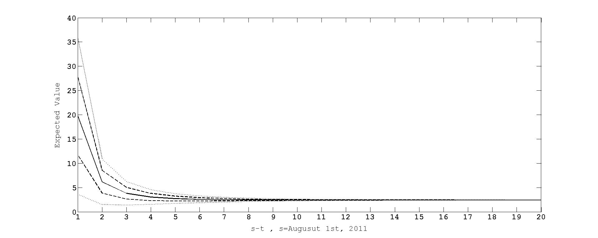
and st𝑠𝑡s-t is the time to maturity. In Benth and Solanilla Blanco [2], a more general study with θ𝜃\theta being a time dependent function concludes that when st0𝑠𝑡0s-t\downarrow 0 the expected value of Z(t,s)𝑍𝑡𝑠Z(t,s) tends to ±plus-or-minus\pm\infty and the variance \infty. Such a case indicates too much dispersion. On the other hand, when st𝑠𝑡s-t\rightarrow\infty, the variance of Z(t,s)𝑍𝑡𝑠Z(t,s) tends to zero, then Z(t,s)𝔼Q(Z(t,s))𝑍𝑡𝑠subscript𝔼𝑄𝑍𝑡𝑠Z(t,s)\approx\mathbb{E}_{Q}(Z(t,s)). Figure. 1 shows the tendency Z(t,s)𝑍𝑡𝑠Z(t,s) when the measurement day s𝑠s is August 1st, 2011.

Refer to caption
Figure 1: Expected value of Z(t,s)𝑍𝑡𝑠Z(t,s) (complete line) as a function of st𝑠𝑡s-t with measurement day s𝑠s being August 1st, 2011. In addition, we have inserted the bounds for ±1plus-or-minus1\pm 1 std (slashed line) and ±2plus-or-minus2\pm 2 std (dotted line).
Refer to caption
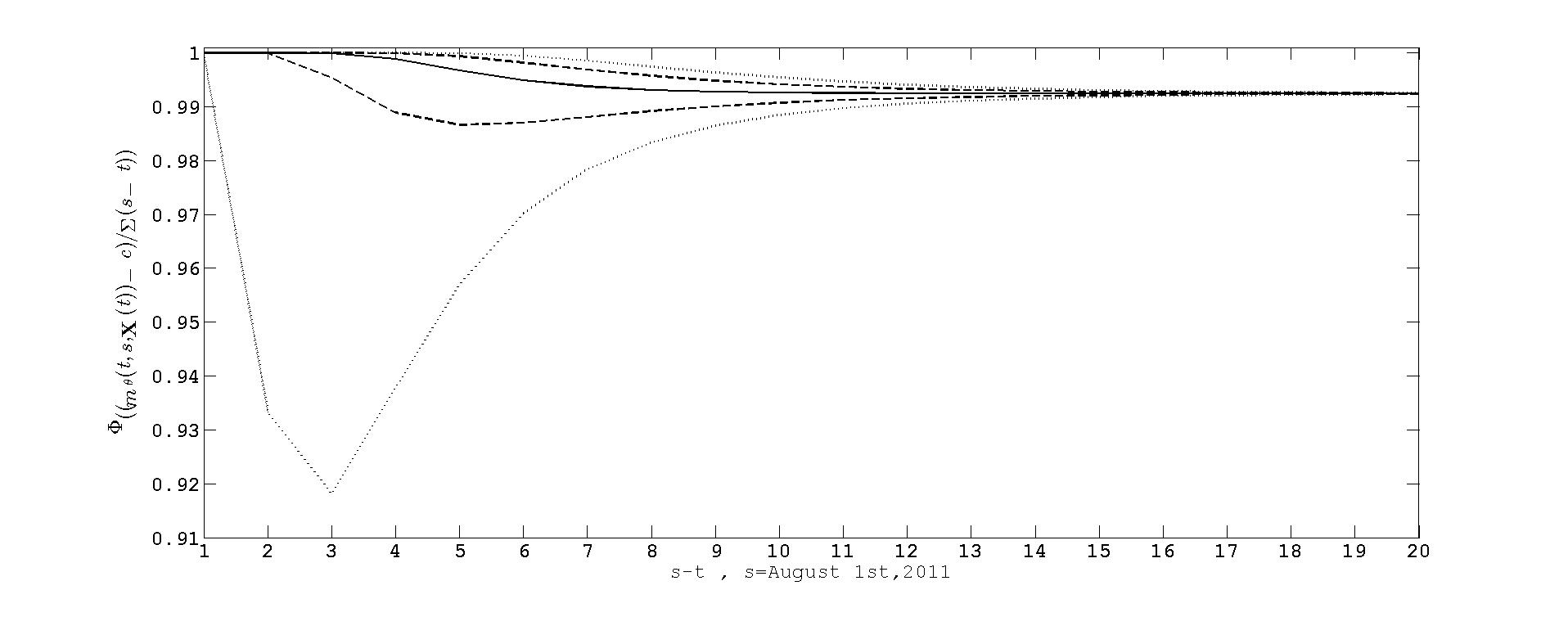
Figure 2: Φ(𝔼Q(Z(t,s)))Φsubscript𝔼𝑄𝑍𝑡𝑠\Phi(\mathbb{E}_{Q}(Z(t,s))) (complete line) as a function of st𝑠𝑡s-t, where we have chosen s𝑠s as August 1st, 2011. In addition, we have inserted Φ(𝔼Q(Z(t,s))±istd)Φplus-or-minussubscript𝔼𝑄𝑍𝑡𝑠𝑖std\Phi(\mathbb{E}_{Q}(Z(t,s))\pm i\,\text{std}) for i=1𝑖1i=1 (slashed line) and i=2𝑖2i=2 (dotted line).

Figure. 2 is the result of applying the function ΦΦ\Phi to the plot in Figure. 1. We see that Φ(Z(t,s))=1Φ𝑍𝑡𝑠1\Phi(Z(t,s))=1 for st=1,2𝑠𝑡12s-t=1,2. From st=3𝑠𝑡3s-t=3 to st=11𝑠𝑡11s-t=11 there is a small decay and finally Φ(Z(t,s))Φ𝑍𝑡𝑠\Phi(Z(t,s)) stabilizes at 0.9924 for st12𝑠𝑡12s-t\geq 12. The values between the dashed lines are more probable than the ones in between the dotted lines. We deduce that

(xiFCDD(t,s,x1,x2,x3))|𝐱=𝐗(t)xiF~CDD(t,s,x1,x2,x3),\big{(}\frac{\partial}{\partial\texttt{x}_{i}}F_{\text{CDD}}(t,s,\texttt{x}_{1},\texttt{x}_{2},\texttt{x}_{3})\big{)}_{|_{\mathbf{x}=\mathbf{X}(t)}}\leq\frac{\partial}{\partial\texttt{x}_{i}}\widetilde{F}_{\text{C}DD}(t,s,\texttt{x}_{1},\texttt{x}_{2},\texttt{x}_{3}),

for i=1,,3𝑖13i=1,\ldots,3 , i.e., the approximate CDD futures prices are more sensitive to changes in the components of 𝐗(t)𝐗𝑡\mathbf{X}(t) than the CDD futures prices.

Recall from Benth and Solanilla Blanco [1] that 𝐗(t)𝐗𝑡\mathbf{X}(t) contains the deseasonalized temperature Y(t)𝑌𝑡Y(t) and its derivatives up to order p1𝑝1p-1. In our setting then, 𝐗(t)𝐗𝑡\mathbf{X}(t) reduces to

𝐗(t)=(Y(t)Y(t)Y′′(t)),𝐗𝑡𝑌𝑡superscript𝑌𝑡superscript𝑌′′𝑡\mathbf{X}(t)=\left(\begin{array}[]{c}Y(t)\\ Y^{\prime}(t)\\ Y^{\prime\prime}(t)\end{array}\right), (4.2)

where Y(t)superscript𝑌𝑡Y^{\prime}(t) and Y′′(t)superscript𝑌′′𝑡Y^{\prime\prime}(t) are respectively the slope and the curvature of Y(t)𝑌𝑡Y(t), respectively.

Refer to caption
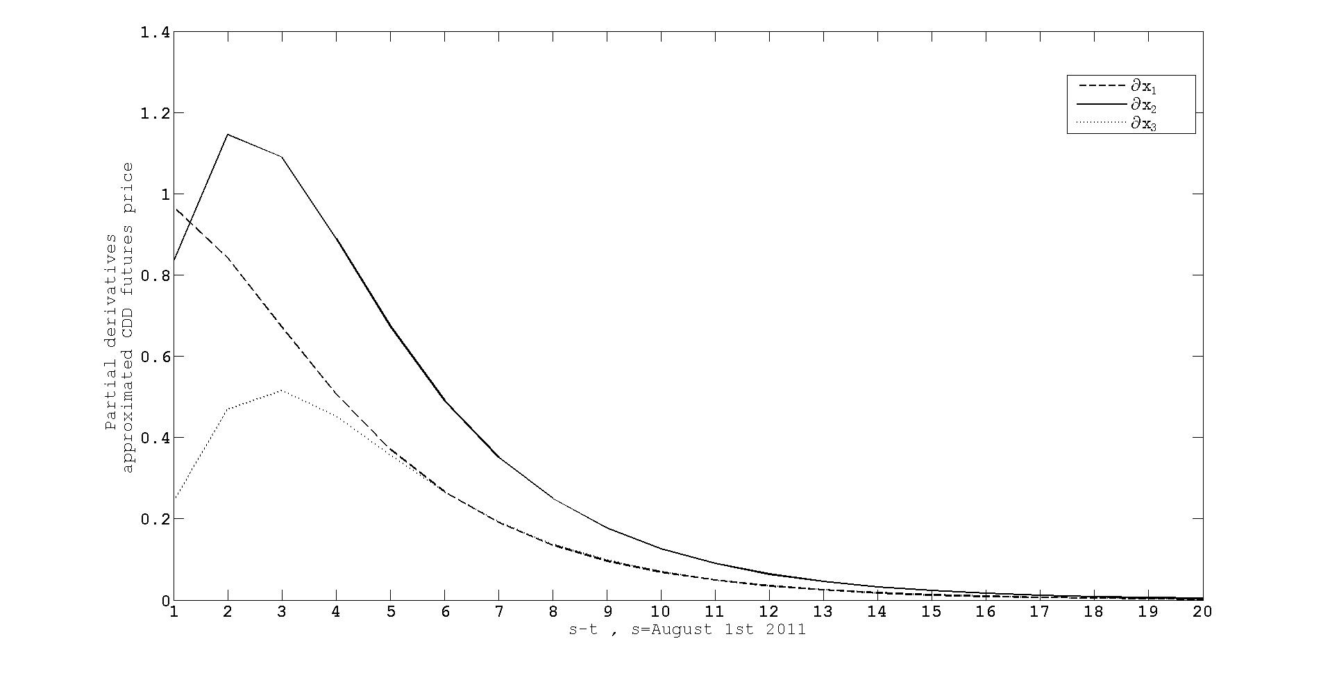
Figure 3: F~CDD(t,s,x1,,xp)/xisubscript~𝐹CDD𝑡𝑠subscriptx1subscriptx𝑝subscriptx𝑖\partial\widetilde{F}_{\text{CDD}}(t,s,\texttt{x}_{1},\ldots,\texttt{x}_{p})/\partial\texttt{x}_{i} for i=1,2,3𝑖123i=1,2,3 as a function of st𝑠𝑡s-t with measurement day s𝑠s being August 1st, 2011.

Figure. 3 shows the partial derivatives of the approximate CDD futures price with respect the coordinates of 𝐱𝐱\mathbf{x} as presented in Proposition. 3.2. The x-axis considers the time to maturity, st𝑠𝑡s-t, where the measurement day s𝑠s is August 1st, 2011. The y-axis shows the different partial derivatives. Firstly, we observe that the partial derivatives of the approximate CDD futures price are positive. We see that at time to maturity st=1𝑠𝑡1s-t=1 any perturbation in the component x1subscriptx1\texttt{x}_{1} affects the tendency of the approximate CDD futures price more than in the components x2subscriptx2\texttt{x}_{2} and x3subscriptx3\texttt{x}_{3}. However, when time to maturity increases the contribution of x1subscriptx1\texttt{x}_{1} decreases gradually. From st=1𝑠𝑡1s-t=1 to st=2𝑠𝑡2s-t=2 the contribution of x2subscriptx2\texttt{x}_{2} increases to the extent that at time to maturity st=2𝑠𝑡2s-t=2 perturbations in x2subscript𝑥2x_{2} dominate the evolution of the approximate CDD futures price. From st>2𝑠𝑡2s-t>2 the contribution of x2subscriptx2\texttt{x}_{2} decreases gradually but it remains always above x1subscriptx1\texttt{x}_{1}. The contribution of x3subscriptx3\texttt{x}_{3} increases from st=1𝑠𝑡1s-t=1 to st=3𝑠𝑡3s-t=3. For bigger times to maturity it decreases gradually. We point out that variations in x3subscriptx3\texttt{x}_{3} always contribute less than variations in x1subscriptx1\texttt{x}_{1} or x2subscriptx2\texttt{x}_{2}. At the long end, small variations in any component hardly affect the tendency of the approximate CDD futures price. This fact makes sense as the term 𝐞1eA(st)𝐱subscript𝐞1superscript𝑒𝐴𝑠𝑡𝐱\mathbf{e}_{1}e^{A(s-t)}\mathbf{x}, which is dependent on the coordinates of 𝐱𝐱\mathbf{x}, tends to zero at the long end. The partial derivatives of the CDD futures price with respect the coordinates of 𝐱𝐱\mathbf{x}, as presented in Proposition. 3.1, depend on 𝐗(t)𝐗𝑡\mathbf{X}(t). The first component Y(t)=T(t)Λ(t)𝑌𝑡𝑇𝑡Λ𝑡Y(t)=T(t)-\Lambda(t) corresponds to the deseasonalized temperature. We approximate the derivatives of Y(t)𝑌𝑡Y(t) with backward finite differences. Hence Y(t)Y(t)Y(t1)superscript𝑌𝑡𝑌𝑡𝑌𝑡1Y^{\prime}(t)\approx Y(t)-Y(t-1) is approximated by the difference between the deseasonalized temperature at times t𝑡t and t1𝑡1t-1. Y′′(t)Y(t)2Y(t1)+Y(t2)superscript𝑌′′𝑡𝑌𝑡2𝑌𝑡1𝑌𝑡2Y^{\prime\prime}(t)\approx Y(t)-2Y(t-1)+Y(t-2) is approximated by a linear combination of the deseasonalized temperatures at times t𝑡t and the two prior times t1𝑡1t-1 and t2𝑡2t-2. Finally, we get the following relation between the temperature and the seasonal function:

(T(t)T(t1)T(t2))matrix𝑇𝑡𝑇𝑡1𝑇𝑡2\displaystyle\begin{pmatrix}T(t)\\ T(t-1)\\ T(t-2)\end{pmatrix} (Λ(t)+Y(t)Λ(t1)+Y(t)Y(t)Λ(t2)+Y′′(t)2Y(t1)+Y(t))|𝐗(𝐭)=𝐱\displaystyle\approx\begin{pmatrix}\Lambda(t)+Y(t)\\ \Lambda(t-1)+Y(t)-Y^{\prime}(t)\\ \Lambda(t-2)+Y^{\prime\prime}(t)-2Y^{\prime}(t-1)+Y(t)\end{pmatrix}_{\Big{|}_{\mathbf{X(t)}=\mathbf{x}}}
=(Λ(t)+x1Λ(t1)+x1x2Λ(t2)+x32x2+x1).absentmatrixΛ𝑡subscriptx1Λ𝑡1subscriptx1subscriptx2Λ𝑡2subscriptx32subscriptx2subscriptx1\displaystyle=\begin{pmatrix}\Lambda(t)+\texttt{x}_{1}\\ \Lambda(t-1)+\texttt{x}_{1}-\texttt{x}_{2}\\ \Lambda(t-2)+\texttt{x}_{3}-2\texttt{x}_{2}+\texttt{x}_{1}\end{pmatrix}. (4.3)

Observe that given a fixed 𝐗(t)𝐗𝑡\mathbf{X}(t) with 0ts0𝑡𝑠0\leq t\leq s, the temperature at time t𝑡t is approximately x1subscriptx1\texttt{x}_{1} degrees above the seasonal mean function and one and tho days prior to t𝑡t, it is approximately x1x2subscriptx1subscriptx2\texttt{x}_{1}-\texttt{x}_{2} and x32x2+x1subscriptx32subscriptx2subscriptx1\texttt{x}_{3}-2\texttt{x}_{2}+\texttt{x}_{1} degrees above the seasonal mean function, respectively.

Consider 𝐗(t)=𝟎𝐗𝑡0\mathbf{X}(t)=\mathbf{0} where 𝟎0\mathbf{0} is the null vector in 3superscript3\mathbb{R}^{3}. The partial derivatives of the CDD futures price are completely deterministic. By the relation between the temperature and the seasonal function established in (4), for this particular case the temperature for the time t𝑡t and the two prior times t1𝑡1t-1 and t2𝑡2t-2 is approximately the seasonal mean function.
Refer to caption
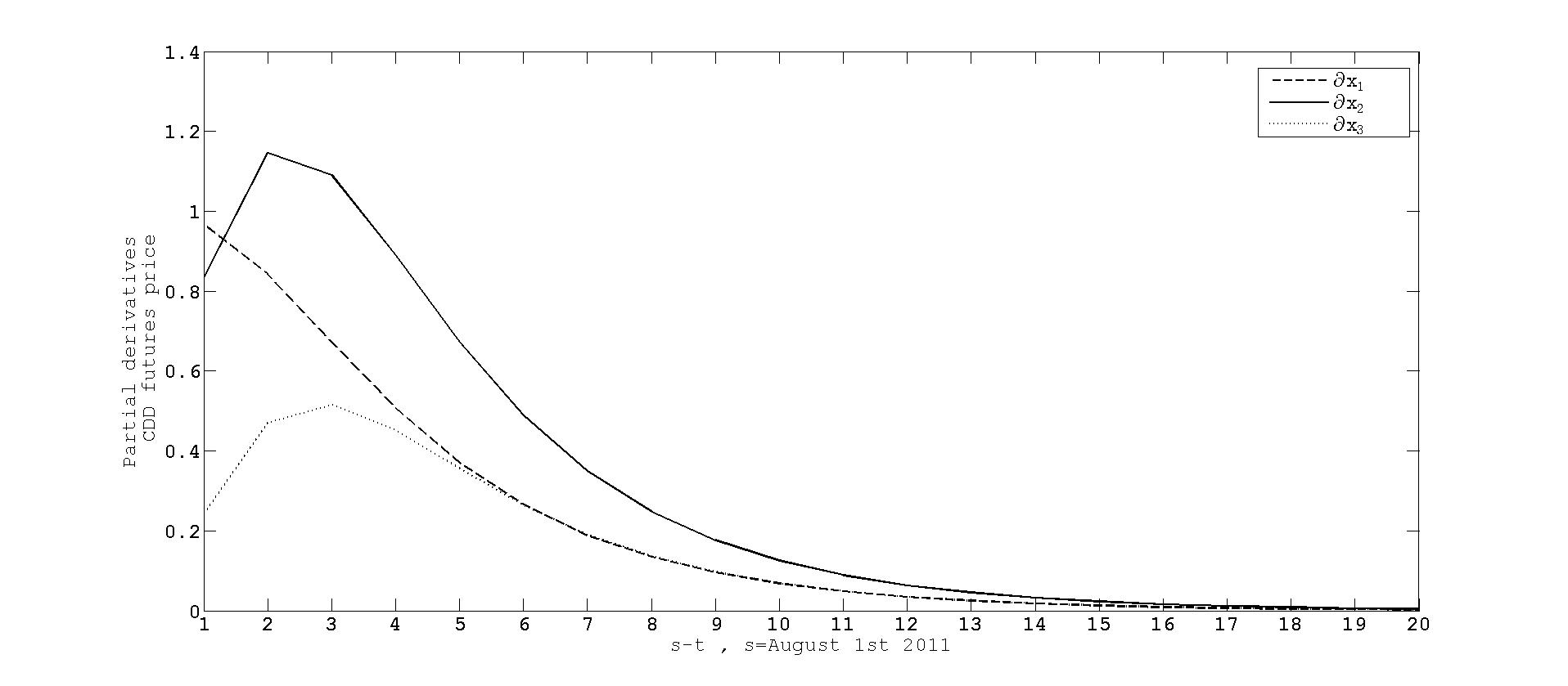
Figure 4: (FCDD(t,s,x1,,xp)/xi)|𝐱=𝟎(\partial F_{\text{CDD}}(t,s,\texttt{x}_{1},\ldots,\texttt{x}_{p})/\partial\texttt{x}_{i})_{|_{\mathbf{x}=\mathbf{0}}} as a function of st𝑠𝑡s-t with measurement day s𝑠s being August 1st, 2011.

Figure. 4 shows the partial derivatives of the CDD futures price with respect the coordinates of 𝐱𝐱\mathbf{x} derived in Proposition 3.1. The x-axis considers the time to maturity, st𝑠𝑡s-t, where the measurement day s𝑠s is August 1st, 2011. The y-axis shows the different partial derivatives.

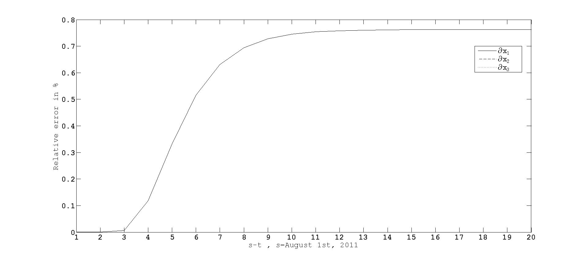
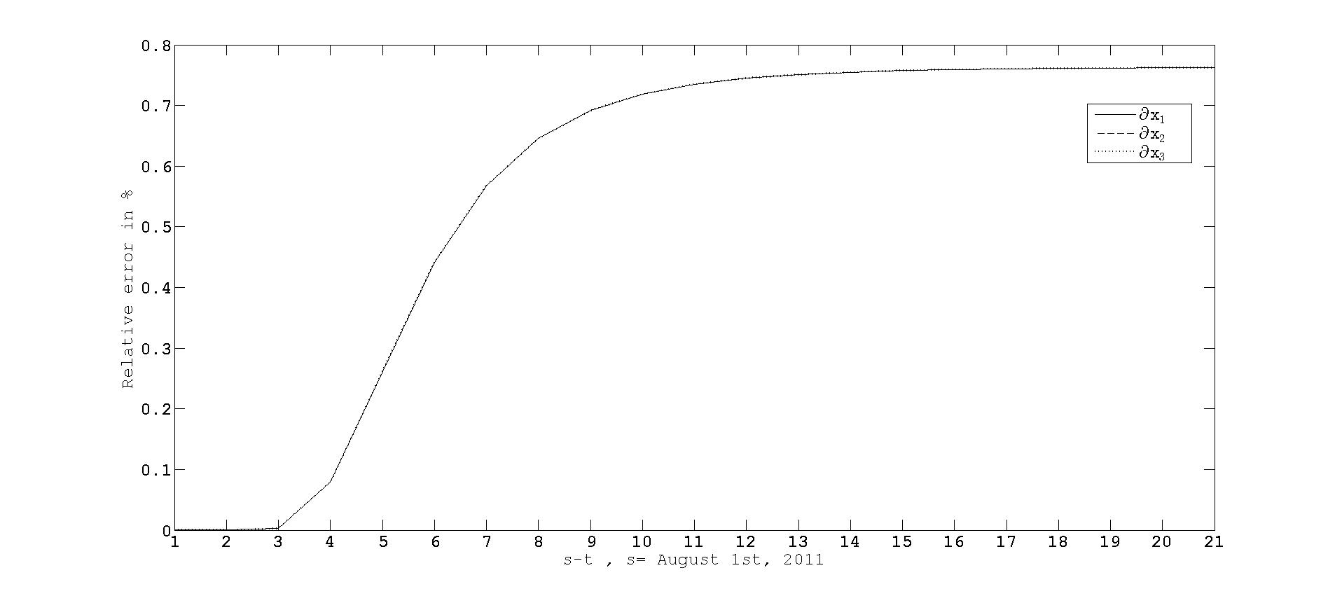
Observe that at first sight Figure. 3 and Figure. 4 seem to coincide. Indeed, Figure. 5 below shows that the relative error between them is less than 1%percent\% entirely.

Refer to caption
Figure 5: The relative error in percent between F~CDD(t,s,x1,,xp)/xisubscript~𝐹CDD𝑡𝑠subscriptx1subscriptx𝑝subscriptx𝑖\partial\widetilde{F}_{\text{CDD}}(t,s,\texttt{x}_{1},\ldots,\texttt{x}_{p})/\partial\texttt{x}_{i} and (FCDD(t,s,x1,,xp)/xi)|𝐱=𝟎(\partial F_{\text{CDD}}(t,s,\texttt{x}_{1},\ldots,\texttt{x}_{p})/\partial\texttt{x}_{i})_{|_{\mathbf{x}=\mathbf{0}}} for i=1,2,3𝑖123i=1,2,3 as a function of st𝑠𝑡s-t with measurement day s𝑠s being August 1st, 2011.

Consider also the case where 𝐗(t)=𝐞k𝐗𝑡subscript𝐞𝑘\mathbf{X}(t)=\mathbf{e}_{k} is the k𝑘kth canonical basis vector in 3superscript3\mathbb{R}^{3} for k=1,,3𝑘13k=1,\ldots,3. For 𝐗(t)=𝐞1𝐗𝑡subscript𝐞1\mathbf{X}(t)=\mathbf{e}_{1} the temperature at the present time t𝑡t and at the two consecutive prior times to t𝑡t, say t1𝑡1t-1 and t2𝑡2t-2, is approximately one degree above the seasonal mean function. For 𝐗(t)=𝐞2𝐗𝑡subscript𝐞2\mathbf{X}(t)=\mathbf{e}_{2}, the temperature is close to the seasonal mean at present time t𝑡t and it is approximately one and two degrees below the seasonal mean at times t1𝑡1t-1 and t2𝑡2t-2, respectively. Finally for 𝐗(t)=𝐞3𝐗𝑡subscript𝐞3\mathbf{X}(t)=\mathbf{e}_{3} the temperature is close to the seasonal mean at present time t𝑡t and one prior time, but two days prior to t𝑡t it is nearly one degree above its seasonal mean. The partial derivatives of the CDD futures price evaluated at the canonical basis vectors in 3superscript3\mathbb{R}^{3} also behave in a similar way to the partial derivatives on the approximate CDD futures price. Figure. 6 below shows that, for the case 𝐗(t)=𝐞1𝐗𝑡subscript𝐞1\mathbf{X}(t)=\mathbf{e}_{1}, the relative error between the partial derivatives of the approximate CDD futures price and the CDD futures price is also less than 1% entirely.
Refer to caption
Figure 6: The relative error in percent between F~CDD(t,s,x1,,xp)/xisubscript~𝐹CDD𝑡𝑠subscriptx1subscriptx𝑝subscriptx𝑖\partial\widetilde{F}_{\text{CDD}}(t,s,\texttt{x}_{1},\ldots,\texttt{x}_{p})/\partial\texttt{x}_{i} and (FCDD(t,s,x1,,xp)/xi)|𝐱=𝐞1(\partial F_{\text{CDD}}(t,s,\texttt{x}_{1},\ldots,\texttt{x}_{p})/\partial\texttt{x}_{i})_{|_{\mathbf{x}=\mathbf{e}_{1}}} for i=1,2,3𝑖123i=1,2,3 as a function of st𝑠𝑡s-t with measurement day s𝑠s being August 1st, 2011.
Refer to caption
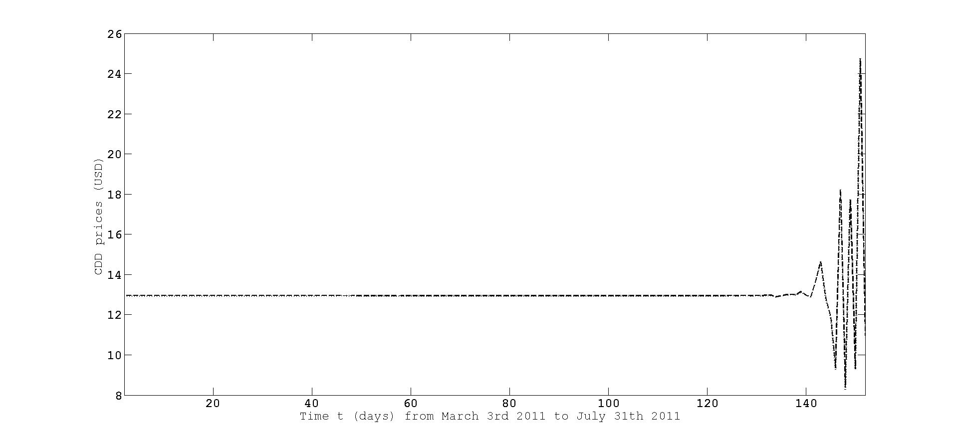
Figure 7: Forward prices and approximate forward prices for CDD contracts from March 3rd, 2011 to July 31th, 2011 with measurement day August 2nd, 2011.

We proceed now with the analysis of call option prices written on CDD futures prices and call option prices written on the approximate CDD futures prices. To do so, we consider the results in Propositons 3.3 and 3.4. Observe that in both results there is dependency on 𝐗(t)𝐗𝑡\mathbf{X}(t). We focus on an at-the-money call option prices. In view of Figure. 7 we fix the strike price K𝐾K being K=13𝐾13K=13.

For the study of the sensitivity of call option prices, we restrict our attention to the cases 𝐗(t)=𝟎𝐗𝑡0\mathbf{X}(t)=\mathbf{0} and 𝐗(t)=𝐞1𝐗𝑡subscript𝐞1\mathbf{X}(t)=\mathbf{e}_{1}. Next, we show the plots with the partial derivatives of the (approximate) call option prices with respect to the coordinates of 𝐱𝐱\mathbf{x} derived in Proposition. 3.3 and Proposition. 3.4.
Refer to caption
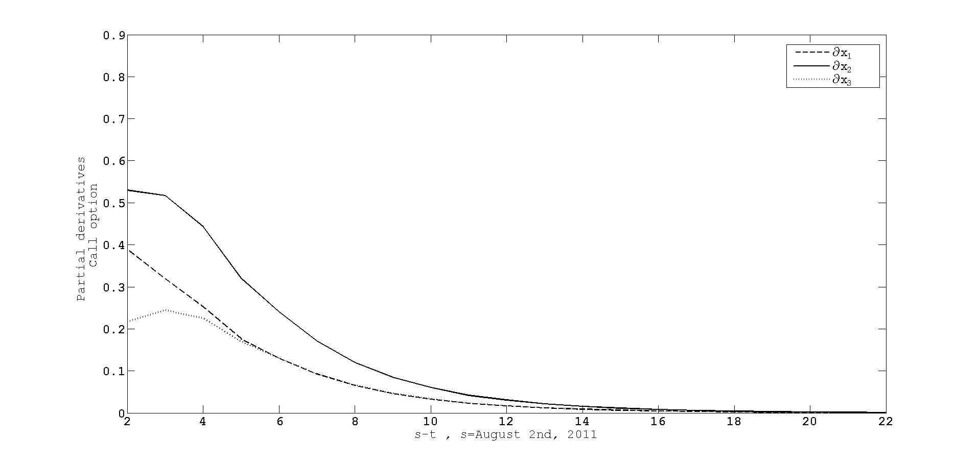
Figure 8: (C(t,τ,s,x1,,xp)/xi)|𝐱=𝟎(\partial C(t,\tau,s,\texttt{x}_{1},\ldots,\texttt{x}_{p})/\partial\texttt{x}_{i})_{|_{\mathbf{x}=\mathbf{0}}} for i=1,2,3𝑖123i=1,2,3 with exercise time τ𝜏\tau being August 1st, 2011 and measurement day s𝑠s August 2nd, 2011.

The x-axis considers the time to maturity, st𝑠𝑡s-t, where s𝑠s is August 2nd, 2011. We have fixed the exercise time τ𝜏\tau being August 1st, 2011. The y-axis shows the different partial derivatives of the call option price when 𝐗(t)=𝟎𝐗𝑡0\mathbf{X}(t)=\mathbf{0}. Firstly, we observe that all the partial derivatives of the call option are positive. We see that for all times to maturity the call option price is more sensitive to any infinitesimal change in the component x2subscriptx2\texttt{x}_{2}, followed by x1subscriptx1\texttt{x}_{1} and x3subscriptx3\texttt{x}_{3}. This tendency follows as time to maturity increases. At the long end, small variations in any component hardly affect the tendency of the call option prices.
Refer to caption
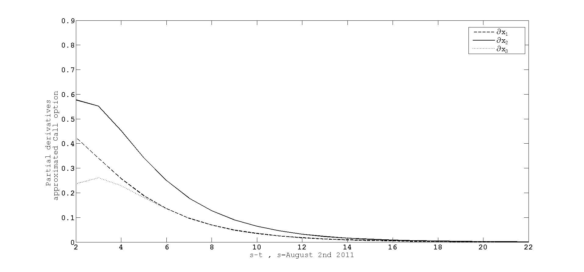
Figure 9: (C~(t,τ,s,F~CDD(t,s,x1,,xp))/xi)|𝐱=𝟎(\partial\widetilde{C}(t,\tau,s,\widetilde{F}_{\text{CDD}}(t,s,\texttt{x}_{1},\ldots,\texttt{x}_{p}))/\partial\texttt{x}_{i})_{|_{\mathbf{x}=\mathbf{0}}} for i=1,2,3𝑖123i=1,2,3 with exercise time τ𝜏\tau being August 1st, 2011 and measurement day s𝑠s August 2nd, 2011.

Figure. 9 shows the partial derivatives of the approximate call option prices with respect to the coordinates of 𝐱𝐱\mathbf{x} derived in Proposition. 3.4 when 𝐗(t)=𝟎𝐗𝑡0\mathbf{X}(t)=\mathbf{0}. We observe that the partial derivatives in Figure. 8 and Figure. 9 show a close habavior. We also see that for small times to maturity the partial derivatives of the approximate call option price are bigger than the partial derivatives of the call option price.

We end our analysis with the results for the case 𝐗(t)=𝐞1𝐗𝑡subscript𝐞1\mathbf{X}(t)=\mathbf{e}_{1}.

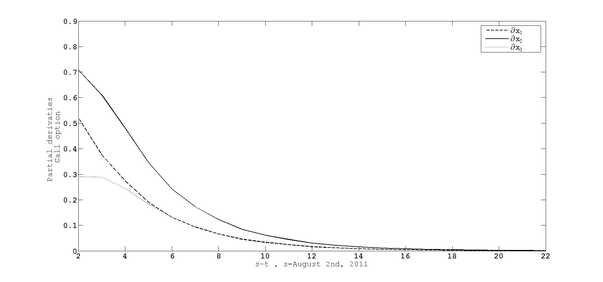
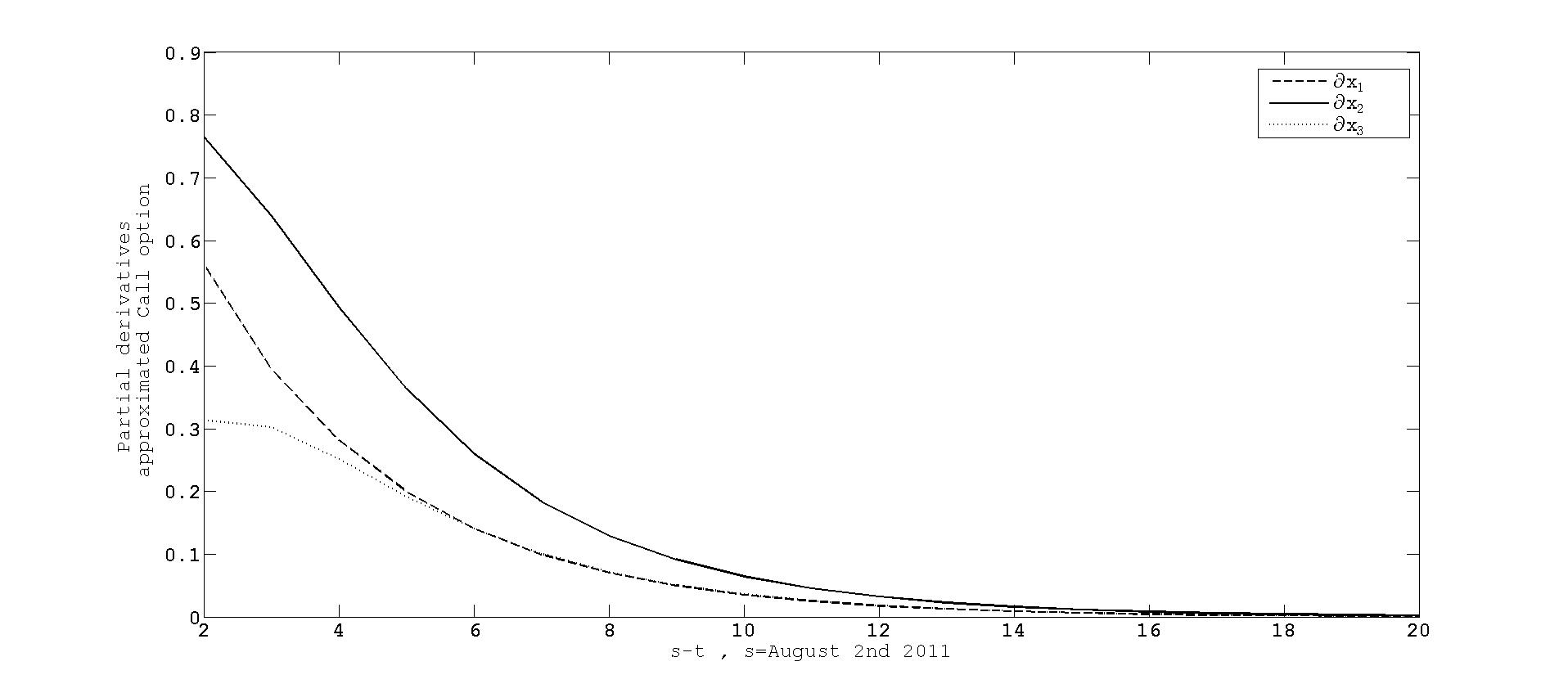
Figure. 10 and Figure.11 show the partial derivatives for the (approximate) call option prices, respectively. We see also here that both prices are more sensitive to changes in the second component of 𝐱𝐱\mathbf{x} in all the domain. Furthermore, the sensitivity to this component decreases as time to maturity increases.
Refer to caption
Figure 10: (C(t,τ,s,x1,,xp))/xi)|𝐱=𝐞1(\partial C(t,\tau,s,\texttt{x}_{1},\ldots,\texttt{x}_{p}))/\partial\texttt{x}_{i})_{|_{\mathbf{x}=\mathbf{e}_{1}}} for i=1,2,3𝑖123i=1,2,3 with exercise time τ𝜏\tau being August 1st, 2011 and measurement day s𝑠s August 2nd, 2011.
Refer to caption
Figure 11: (C~(t,τ,s,F~CDD(t,s,x1,,xp))/xi)|𝐱=𝐞𝟏(\partial\widetilde{C}(t,\tau,s,\widetilde{F}_{\text{CDD}}(t,s,\texttt{x}_{1},\ldots,\texttt{x}_{p}))/\partial\texttt{x}_{i})_{|_{\mathbf{x}=\mathbf{e_{1}}}} for i=1,2,3𝑖123i=1,2,3 with exercise time τ𝜏\tau being August 1st, 2011 and measurement day s𝑠s August 2nd, 2011.

5 Sensitivity of CDD futures prices with measurement over a period

The sensitivity analysis of CDD future prices with measurement over a period [τ1,τ2]subscript𝜏1subscript𝜏2[\tau_{1},\tau_{2}] with respect to infinitesimal changes in the components of 𝐗(t)𝐗𝑡\mathbf{X}(t) can be performed by means of the partial derivatives provided in Proposition.2.1 and Proposition. 2.2. We proceed analogously as in the previous section for CDD futures prices with a measurement day.

The random variable Φ(Z(t,s))Φ𝑍𝑡𝑠\Phi(Z(t,s)) with Z(t,s)𝑍𝑡𝑠Z(t,s) in (4.1) makes here also the difference between the results provided in both Propositions. The same reasoning followed for CDD future prices with a measurement day is valid to conclude that

(xiFCDD(t,τ1,τ2,x1,x2,x3))|𝐱=𝐗(t)xiF~CDD(t,τ1,τ2,x1,x2,x3).\big{(}\frac{\partial}{\partial\texttt{x}_{i}}F_{\text{CDD}}(t,\tau_{1},\tau_{2},\texttt{x}_{1},\texttt{x}_{2},\texttt{x}_{3})\big{)}_{|_{\mathbf{x}=\mathbf{X}(t)}}\leq\frac{\partial}{\partial\texttt{x}_{i}}\widetilde{F}_{\text{C}DD}(t,\tau_{1},\tau_{2},\texttt{x}_{1},\texttt{x}_{2},\texttt{x}_{3}). (5.1)

Hence, the approximate CDD futures price becomes more sensitive to any infinitesimal change in the coordinates of 𝐗(t)𝐗𝑡\mathbf{X}(t) than the CDD futures price.

Refer to caption
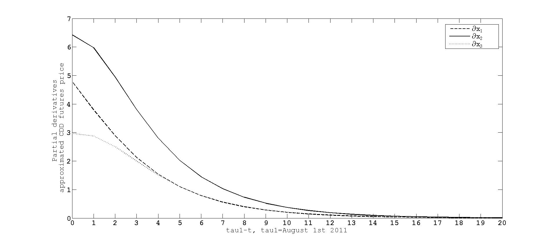
Figure 12: F~CDD(t,τ1,τ2,x1,,xp)/xisubscript~𝐹CDD𝑡subscript𝜏1subscript𝜏2subscriptx1subscriptx𝑝subscriptx𝑖\partial\widetilde{F}_{\text{CDD}}(t,\tau_{1},\tau_{2},\texttt{x}_{1},\ldots,\texttt{x}_{p})/\partial\texttt{x}_{i} as a function of τ1tsubscript𝜏1𝑡\tau_{1}-t with measurement period [τ1,τ2]subscript𝜏1subscript𝜏2[\tau_{1},\tau_{2}] being August, 2011.

Figure.12 shows the partial derivatives of the approximate CDD futures price with respect the coordinates of 𝐱𝐱\mathbf{x} derived in Proposition. 2.2.

The x-axis considers the time to maturity, τ1tsubscript𝜏1𝑡\tau_{1}-t, where τ1subscript𝜏1\tau_{1} is August 1st, 2011 and the measurement period [τ1,τ2]subscript𝜏1subscript𝜏2[\tau_{1},\tau_{2}] is August 2011. The y-axis shows the different partial derivatives of the approximate CDD futures price. Firstly, we observe that the values here of the partial derivatives are greater than those corresponding to the partial derivatives of the approximate CDD futures price with a measurement day, with more emphasis on times t𝑡t which are close to τ1subscript𝜏1\tau_{1}. Indeed, the partial derivatives of the approximate CDD futures prices can be understood as the partial derivatives of the approximate CDD futures prices with measurement day s𝑠s which runs over [τ1,τ2]subscript𝜏1subscript𝜏2[\tau_{1},\tau_{2}] as shown as follows

xiF~CDD(t,τ1,τ2,x1,,xp)=τ1τ2xiF~CDD(t,s,x1,,xp)𝑑s.subscriptx𝑖subscript~𝐹CDD𝑡subscript𝜏1subscript𝜏2subscriptx1subscriptx𝑝superscriptsubscriptsubscript𝜏1subscript𝜏2subscriptx𝑖subscript~𝐹CDD𝑡𝑠subscriptx1subscriptx𝑝differential-d𝑠\frac{\partial}{\partial\texttt{x}_{i}}\widetilde{F}_{\text{CDD}}(t,\tau_{1},\tau_{2},\texttt{x}_{1},\ldots,\texttt{x}_{p})=\int_{\tau_{1}}^{\tau_{2}}\frac{\partial}{\partial\texttt{x}_{i}}\widetilde{F}_{\text{CDD}}(t,s,\texttt{x}_{1},\ldots,\texttt{x}_{p})\,ds\,.

Recall that Figure. 3 shows that the derivatives of the approximate CDD futures price with a measurement day are positive and when time to maturity increases tend to zero. This fact together with the relation in (5.1) let us to justify why the derivatives of the approximate CDD futures prices with measurement over a period behave in this way. We also observe that any infinitesimal change in x2subscriptx2\texttt{x}_{2} dominates more the behaviour of the approximate CDD futures price, followed by any change in x1subscriptx1\texttt{x}_{1} and x3subscriptx3\texttt{x}_{3}. This was exactly the same tendency followed by the partial derivatives of the approximate CDD futures price with a measurement day, see Figure. 3, for times to maturity greater than 2.

For the study of the sensitivity of the partial derivatives of the CDD futures price with measurement over a period derived in Proposition. 2.1 we consider the cases 𝐗(t)=𝟎𝐗𝑡0\mathbf{X}(t)=\mathbf{0} and 𝐗(t)=𝐞1𝐗𝑡subscript𝐞1\mathbf{X}(t)=\mathbf{e}_{1}.

Refer to caption
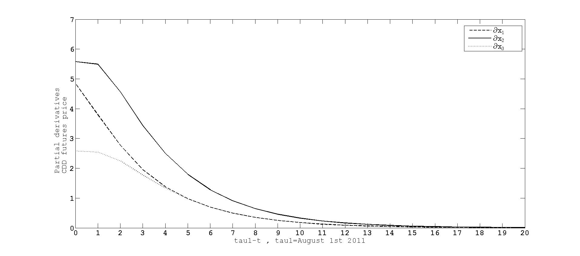
Figure 13: (FCDD(t,τ1,τ2,x1,,xp)/xi)|𝐱=𝟎(\partial F_{\text{CDD}}(t,\tau_{1},\tau_{2},\texttt{x}_{1},\ldots,\texttt{x}_{p})/\partial\texttt{x}_{i})_{|_{\mathbf{x}=\mathbf{0}}} for i=1,2,3𝑖123i=1,2,3 as a function of τ1tsubscript𝜏1𝑡\tau_{1}-t with measurement over a period [τ1,τ2]subscript𝜏1subscript𝜏2[\tau_{1},\tau_{2}] being August, 2011.
Refer to caption
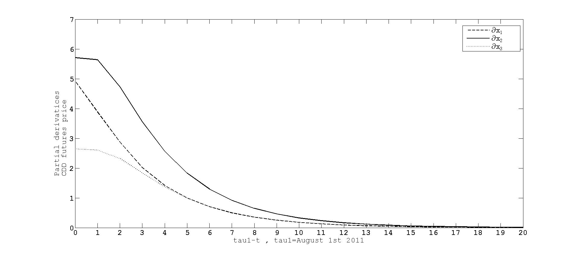
Figure 14: (FCDD(t,τ1,τ2,x1,,xp)/xi)|𝐱=𝐞1(\partial F_{\text{CDD}}(t,\tau_{1},\tau_{2},\texttt{x}_{1},\ldots,\texttt{x}_{p})/\partial\texttt{x}_{i})_{|_{\mathbf{x}=\mathbf{e}_{1}}} for i=1,2,3𝑖123i=1,2,3 as a function of τ1tsubscript𝜏1𝑡\tau_{1}-t with measurement over a period [τ1,τ2]subscript𝜏1subscript𝜏2[\tau_{1},\tau_{2}] being August, 2011.

Figure. 13 and Figure. 14 show also that perturbations in x2subscriptx2\texttt{x}_{2} affect also more in these cases the CDD futures price.

6 Conclusions

In this paper we have studied the local sensitivity of the (approximate) CDD and HDD futures and options prices with respect to a perturbation in the deseasonalized temperature or in one of its derivatives up to a certain order, determined by the CAR process modelling the deseasonalized temperature. We have considered the partial derivatives of these financial contracts with respect to these variables (deseasonalized temperature and its derivatives). The HDD and CDD futures and call option prices and their approximate formulas were derived in Benth and Solanilla Blanco [2]. We have considered and empirical analysis where we have taken the same CAR(3)-process fitted to the time series of New York temperatures in Benth and Solanilla Blanco [2]. The sensitivity study of these financial contracts with a fixed measurement day shows first that the approximate futures prices are more sensitive to any perturbation in one of these variables than the theoretical futures prices. Nevertheless, the relative error between both partial derivatives is rather small. We also observe that one time prior to the considered measurement day the behaviour of the (approximate) futures prices is more affected by a perturbation in the deseasonalized temperature. As time to maturity increases then a perturbation in the slope of the deseasonalized temperature dominates the behaviour of both futures prices. At the long end any perturbation of these variables hardly affect their behaviour. For the call option prices we also observe that the approximate model is more sensitive to any pertubation in one of the previous variables than the theoretical model. We emphasize that unlike futures prices, any perturbation in the slope of the deseasonalized temperature, dominates the behaviour of the call option prices. We have also extended the analysis of sensitivity to futures prices with measurement over a fixed month. We have seen that in this case the slope of the deseasonalized temperature dominates the bahaviour in all the domain.

References

  • [1] F. E. Benth and S. A Solanilla Blanco. Forward prices in markets driven by continuous-time autoregressive processes. In Recent Advances in Financial Engineering: Proceedings of the International Workshop on Finance 2012, pages 1–24, Singapore, 30–31 October 2012 2014. World Scientific.
  • [2] F. E. Benth and S. A Solanilla Blanco. Approximation of the price dynamics of heating degree day and cooling degree day temperature futures. The Journal of Energy Markets., 8:69–92, 2015.
  • [3] F. E. Benth and J Šaltytė Benth. Modeling and Pricing in Financial Markets for Weather Derivatives, volume 17 of Advanced series on statistical science & applied probability. World Scientific, Singapore, 2012.
  • [4] M. Broadie and P Glasserman. Estimating security price derivatives using simulation. Management Science., 42:269–285, 1996.
  • [5] G.B Folland. Real Analysis: Modern Techniques and Their Applications. Advanced series on statistical science & applied probability. Wiley, Chicheter, 1984.
  • [6] W. Härdle and B López Cabrera. The implied market price of weather risk. Appl. Math. Finance., 19:59–95, 2012.