Learning a Generalized Physical Face Model From Data

Abstract.

Physically-based simulation is a powerful approach for 3D facial animation as the resulting deformations are governed by physical constraints, allowing to easily resolve self-collisions, respond to external forces and perform realistic anatomy edits. Today’s methods are data-driven, where the actuations for finite elements are inferred from captured skin geometry. Unfortunately, these approaches have not been widely adopted due to the complexity of initializing the material space and learning the deformation model for each character separately, which often requires a skilled artist followed by lengthy network training. In this work, we aim to make physics-based facial animation more accessible by proposing a generalized physical face model that we learn from a large 3D face dataset. Once trained, our model can be quickly fit to any unseen identity and produce a ready-to-animate physical face model automatically. Fitting is as easy as providing a single 3D face scan, or even a single face image. After fitting, we offer intuitive animation controls, as well as the ability to retarget animations across characters. All the while, the resulting animations allow for physical effects like collision avoidance, gravity, paralysis, bone reshaping and more.

Figure 1. We present a deep generalized physical face model that can be fit to a single face image or 3D scan. The model produces an identity-specific material space with bones, skin and soft tissue, together with per-expression jaw transformations and element actuations for facial simulation. Once fit to an unseen identity, the model can be animated to create physics-based facial animation. Applications like retargeting, interpolation, anatomy editing, and physical effects such as collision avoidance and muscle paralysis are shown in Sec. 6.

1. Introduction

For decades, 3D facial animation has continued to be a challenging and well-studied problem in computer graphics. The quest for more realistic facial motion continues because believable 3D characters are one of the leading contributors to widespread adoption of CG content in films, video games and virtual environments. The reverse is also true, in that unrealistic 3D characters can lead to a widespread rejection of the CG content, which is what makes high-quality facial animation so critical. Most often, faces are parameterized and controlled by linear blendshape rigs, which are popular due to their simplicity and ease of use. Unfortunately, blendshape rigs suffer from well-known drawbacks like providing only linear motion and exhibiting surface inter-penetrations (particularly around the lips). An alternative, and more physically accurate approach is to use physical simulation for facial animation, where anatomical muscle actuations drive the soft tissue deformation. As a benefit, within a simulator it is easy to add constraints to identify surface contacts and prevent collisions, while producing more natural nonlinear face motion. Originally, physics-based methods were popular only in academic settings due to their complexity of adoption in production, however recently more anatomical and physics-inspired approaches have gained popularity in the film industry (Choi et al., 2022).

There are generally two approaches to physics-based facial animation. In the first-principles-based method, researchers model the muscle actuation mechanism according to the authentic complex muscle structures in the face, either obtained through CT/MRI (Sifakis et al., 2005) or an off-the-shelf muscle template (Ichim et al., 2017; Bao et al., 2018). Although physiologically sound, this strategy is laborious, and its realism highly depends on the accuracy of the anatomical model. As such, a second approach emerged based on shape targeting (Klár et al., 2020), where fine-grained and structure-agnostic actuation is inferred from the captured skin geometry and used to target the undeformed soft tissue (Srinivasan et al., 2021; Yang et al., 2022, 2023). Since only the skin geometry and skeleton are required to learn the model, this method largely eases the modeling labor while assuming great flexibility, high fidelity, and improved realism.

While the shape targeting approach is attractive, it is currently only tractable for a few hero characters in a production. This limitation stems from two aspects. First, although the modeling effort is less than a first-principles approach, there is still a dedicated setup procedure required for each character. This involves scanning and tracking a dataset of facial geometry from the actor in various expressions, building a simulation-ready material space to model the soft tissue and bones at rest, and then training a dedicated neural network to predict the muscle actuations for each expression-dependent deformation. Secondly, there is a time-consuming, memory-intensive, and identity-specific differentiable simulation in the training loop. It would be infeasible to train many character-specific networks within a reasonable amount of time and resources, using the currently-available architectures for soft-tissue-based physical face animation.

In this work we aim to alleviate these issues and make physics-based facial animation more freely accessible. To this end, we propose a new, generalized physical face model that can be easily adapted to any new character without manual setup costs. We accomplish this by learning a single implicit neural model for actuation mechanisms trained on a large dataset of hundreds of identities performing a variety of expressions. Naturally, the above-mentioned limitations would pose a considerable problem for this approach as each identity would require a personalized material space and training on such a large dataset with simulation in the loop would be impossible. We overcome these hurdles with our two main contributions. First, we propose a design that allows for simulation-free training, which is fast and memory efficient, allowing us to train on a large dataset of faces and learn the generalizability one would need for such an application. Second, we propose an architecture that automatically predicts an identity-conditioned material space by warping a single canonical material space. Despite not having simulation in the training loop nor hand-crafted per-identity material spaces, our network still produces outputs that are compatible with a physics simulator, such that the resulting faces can be animated using physics-based facial animation.

Our model is conditioned on two latent codes, one for identity and one for expression, and the output is an identity-specific material space (i.e., skull, jaw, skin and soft tissue in between) coupled with identity- and expression-specific actuations and bone kinematics that can all be readily provided to an off-the-shelf physics simulator. As a result, our pre-trained network can be used to generate an animation-ready physics-based simulation model for any new character, simply by modifying the identity latent code. We demonstrate that our model can be fit to a single 3D neutral scan of an actor, or even simply to a single face image. Once fitted, the model allows animation through the controls of a common 3D morphable face model, which are mapped to our latent space. Furthermore, our method supports animation retargeting by swapping identity codes. In all cases, the resulting animation benefits from physical effects like the detection of surface contacts and collision avoidance, the ability to paralyze parts of the face, edit anatomical bone structures, and obey gravitational or other external forces.

In summary, we propose a physical face model that is as generalizable and controllable as current linear blendshape models, but with the added benefit of more physically-accurate facial deformations. We believe our work will help to democratize physics-based facial animation, making it as simple as fitting an animation-ready simulation model to a single scan or image.

2. Related Work

Facial models used in animation range from simple global linear shape models to complex local models that incorporate the underlying facial anatomy through anatomical constraints or physical simulation. We will focus our discussion on anatomical face models and the generation of 3D face models from monocular input.

2.1. Physics-Based Facial Animation

Physics-based facial animation typically employs two main approaches. The first, known as the first-principles-based method, requires users to intricately model the muscle actuation mechanism based on the complex structures of facial muscles. These structures are derived from sources such as CT/MRI scans (Sifakis et al., 2005) or pre-existing muscle templates (Ichim et al., 2017; Bao et al., 2018). While this approach ensures physiological accuracy, the generation of such models is labor-intensive and the realism of the resulting animation heavily relies on the precision of the anatomical and biomechanical models.

In response to the challenges posed by the first-principles-based method, a second approach has emerged, known as shape targeting (Klár et al., 2020). In this methodology, every element within the mesh is considered active and subject to actuation for the purpose of inducing forces that drive the motion of the face or body. To reproduce identity-specific facial expressions, an actuation mechanism is optimized based on face capture data. In the work of Srinivasan et al. (2021), the integration of neural networks with a comprehensive muscle model facilitated the learning of the muscle actuation mechanism. Subsequent advancements in the field transitioned towards an implicit neural representation, rendering the actuation mechanism more compact and independent of resolution (Yang et al., 2022). Building upon this foundation, Yang et al. (2023) further extended the methodology by training the neural network on captured data from a small number of individuals simultaneously. This multi-identity training approach enables the model to learn diverse expression styles based on distinct actuation patterns and allows applications such as style retargeting.

Notably, these actuation-based approaches streamline the modeling process by only necessitating skin geometry and bone data for model training. Nevertheless, their heavy reliance on identity-specific data, hand-crafted material spaces and architectures that only allow training on one or few identities at a time represent significant limitations, particularly hindering their generalizability and widespread application in production settings. We address this by introducing a generalized physical face model that can be easily adapted to any new character.

The recent work of Wagner et al. (2023) is the closest in spirit to our work, as we share a common motivation although very different solutions. They propose an extension to linear blendshape models that aims to mimic physics-based facial animation within a linear framework. Physical simulation is only used to generate training data, not at runtime, and thus they are tied to the prescribed simulation effects present in the dataset. For example, they cannot handle lip collisions, which is a primary reason to employ simulation for facial animation. On the other hand, we propose a nonlinear physics-based face model trained on real capture data, which can be fit to any novel identity and provide a true physical model that employs simulation at runtime to allow any desired physical effect, including lip collision avoidance.

2.2. Anatomically-Constrained Face Models

Anatomical constraints on the facial surface are often used to plausibly restrict the range of the skin deformations. The anatomically-constrained local deformation model, introduced in the context of monocular facial performance capture by Wu et al. (2016), initially established a connection between the skin surface and anatomical bones. This was achieved by modeling the thickness of the soft tissue between a bone point and the skin surface, together with skin sliding coupled with bulging. This anatomically-constrained face model was also beneficial in face modeling applications, helping untrained users to quickly create believable digital characters (Gruber et al., 2020). In the domain of facial performance retargeting, Chandran et al. (2022) employed the same model to confine a retargeted shape within the realm of anatomically plausible shapes specific to a target actor. An implicit variant of the anatomical face model was presented by Chandran and Zoss (2023), which facilitates the learning of a continuous anatomical structure that densely constrains the skin surface. The model can disentangle deformation arising from rigid bone motion and non-rigid deformations created by muscle activations. Qiu et al. (2022) learned an anatomical facial shape model from medical imaging data, and presented a morphable model that is able to generate faces that jointly model the skull, facial surface and appearance. Choi et al. (2022) replaced the muscle-based parameterization used earlier (Sifakis et al., 2005; Srinivasan et al., 2021) by a collection of muscle fiber curves, whose contraction and relaxation provide a fine-grained parameterization of human facial expression. The approach strikes a balance between the requirements for anatomically-based and artist-friendly models, but comes at the expense of reduced physical accuracy, as the simulation is solely employed in a pre-processing step to acquire an approximate deformation model of muscle fibers.

Similarly, our approach is designed for ease of usability, as it shares the generality and controllability characteristics found in existing linear blendshape models, yet it offers the additional advantage of achieving more physically accurate facial deformation.

2.3. Morphable 3D Face Models

As our generalized physical face model is driven by identity and expression and produces a deformed 3D face as the output, it is akin to traditional 3D morphable face models in current literature (Blanz and Vetter, 1999; Li et al., 2017; Dai et al., 2019; Yang et al., 2020a; Chai et al., 2022), with the main difference that ours allows to simulate physical effects. A common application of most 3DMMs is their use in monocular face reconstruction, e.g., fitting the model to images. As such, we present a high-level summary of existing techniques where a morphable model is used to recover a person’s facial geometry in 3D either by directly optimizing the face shape based on an observed image or through an inference-driven approach that trains neural networks to predict the parameters of a morphable model.

Determining the optimal 3DMM shape, expression, and pose parameters for a given RGB image is achieved through either analysis-by-synthesis optimization (Gecer et al., 2019, 2021) or deep neural network regression (Feng et al., 2021; Zielonka et al., 2022; Zhang et al., 2023). Recently, there have also been several approaches that rely on additional perception based loss terms to improve the visual quality of these morphable model fits (Danecek et al., 2022; Filntisis et al., 2022; Otto et al., 2023).

Comprehensive surveys on 3DMMs and their application in monocular face capture are provided by Egger et al. (2020), and Morales et al. (2020). As an application of our generalized physical face model we also show the ability to fit the model to unseen identities in the form of a single face image. However, we do not propose a competing method for accurate 3D geometry reconstruction but rather a convenient approach to obtain an animation-ready physical model, using a similar fitting approach as in the field of monocular face capture.

3. Preliminaries: Actuated Face Simulation

In continuum mechanics, motion is characterized by an invertible map $\phi:\mathbf{X}\in\Omega^{0}\rightarrow\mathbf{x}\in\Omega$ from the undeformed material space $\Omega^{0}$ to the deformed space $\Omega$. The deformation gradient, $\mathbf{F}(\mathbf{X})=\nabla_{\mathbf{X}}\phi(\mathbf{X})$, encodes the local transformations including rotation and stretch. The quasi-static state of $\phi$ in the absence of external force is governed by the point-wise equilibrium:

(1) $$\operatorname{div}\cdot\,\mathbf{P}=\operatorname{div}\cdot\,\frac{\partial\Psi}{\partial\mathbf{F}}(\mathbf{F})=\mathbf{0},$$

where $\mathbf{P}$ is the first Piola–Kirchhoff stress tensor that measures the internal force. For hyperelastic material, $\mathbf{P}$ is associated with a specific energy density function $\Psi$ that describes the material behavior. Intuitively, Eqn. (1) means the net force within the material is zero everywhere.

In the context of actuated face simulation, the material space $\Omega^{0}$ is defined as the undeformed soft tissue space confined between the rest bones $\partial\Omega_{\text{bones}}^{0}$ and skin $\partial\Omega_{\text{skin}}^{0}$. $\partial\Omega_{\text{bones}}^{0}$ consists of the skull $\partial\Omega_{\text{skull}}^{0}$ and the jaw $\partial\Omega_{\text{jaw}}^{0}$, which will constrain and drag the soft tissue during articulation. The deformed space $\Omega$ is the soft tissue space of the target expression. For $\Psi$, the shape targeting model (Klár et al., 2020) is employed:

(2) $$\Psi(\mathbf{F},\mathbf{A})=\underset{\mathbf{R}\in\mathrm{SO}(3)}{\operatorname{min}}||\mathbf{F}-\mathbf{R}\mathbf{A}||^{2}_{F}=||\mathbf{F}-\mathbf{R}^{*}\mathbf{A}||^{2}_{F},$$

where $\mathbf{A}$ is a symmetric actuation tensor mimicking the local muscle actuation. $\mathbf{R}^{*}$ is the polar decomposition of $\mathbf{F}\mathbf{A}$, making $\Psi$ rotationally-invariant. Based on embedded simulation, $\Omega^{0}$ is uniformly discretized into a simulation mesh $\mathcal{M}_{\text{sim}}$ using regular elements with nodal vertices $\mathbf{u}^{0}$, where the discretized skin, skull and jaw are linearly embedded with barycentric weights $\mathbf{W}_{s}\mathbf{u}^{0}$, $\mathbf{W}_{m}\mathbf{u}^{0}$, and $\mathbf{W}_{n}\mathbf{u}^{0}$ respectively. With the Finite Element Method (FEM) applied to Eqn. (1), the simulation then reduces to an energy minimization problem w.r.t. the deformed vertices $\mathbf{u}$ such that the boundary conditions from the articulated bone are satisfied, as follows:

(3) $$\underset{\mathbf{u}}{\operatorname*{argmin}}\sum_{e}\frac{V_{e}}{2}||{\mathbf{F}}_{e}(\mathbf{u},\mathbf{u}^{0})-\mathbf{R}_{e}^{*}\mathbf{A}_{e}||_{F}^{2}$$

(10) $$\operatorname{s.t.}\;\left[\begin{array}[]{l}\mathbf{W}_{m}\\ \mathbf{W}_{n}\\ \end{array}\right]\mathbf{u}=\left[\begin{array}[]{l}\mathbf{W}_{m}\\ \mathbf{R}_{\text{jaw}}\mathbf{W}_{n}\\ \end{array}\right]\mathbf{u}^{0}+\left[\begin{array}[]{l}\mathbf{0}\\ \mathbf{t}_{\text{jaw}}\\ \end{array}\right],$$

where $V_{e}$ is the volume for each element $e$ while $\{\mathbf{R}_{\text{jaw}},\mathbf{t}_{\text{jaw}}\}$ denotes the rigid transformation for the jaw.

In summary, the simulation entails three core elements:

• Identity material space ($\Omega^{0}$) to get $\mathcal{M}_{\text{sim}}$ with embedded skin, skull, and jaw.

• Facial actuation defined by the tensor field $\mathcal{A}$ over $\mathcal{M}_{\text{sim}}$.

• Jaw kinematics via mandible transformation $\{\mathbf{R}_{\text{jaw}},\mathbf{t}_{\text{jaw}}\}$.

The latter two components function as muscle actuation mechanisms and are utilized as the input physical constraints. This simulation process can be made efficiently differentiable with the adjoint method, allowing inverse design of $\mathcal{A}$ and $\{\mathbf{R}_{\text{jaw}},\mathbf{t}_{\text{jaw}}\}$ from a target expression of the identity. However, the expensive computation from the simulation and the requirement of the pre-defined material space $\Omega^{0}$ prevent this method from lending itself to a large face dataset of hundreds of identities, where the identity-specific material space (underlying anatomy) is typically missing.

4. Method

Figure 2. Overview of our model. Driven by identity $\beta$ and expression $\gamma$ latent codes, $\mathcal{N}_{C}$ learns to deform a canonical material space $\Omega^{C}$ to be identity-specific, $\Omega^{0,\beta}$. Then $\mathcal{N}_{e}$ learns to deform the material space to match a given expression, $\Omega^{\gamma,\beta}$. The latent codes are parameterized by a common 3DMM ($\hat{\beta}$, $\hat{\gamma}$). The network is trained with physically-inspired constraints so that, after discretization, a simulator will produce physics-based facial animation.

Our goal is to build a generalized physical face model from a large 3D face dataset where only skin geometry is given. This face model should be generative and animatable, such that it can be fit to a variety of input data (e.g., 3D scans or face images) and then animated with intuitive controls, providing a convenient mechanism to obtain a physical face model for animation purposes.

To achieve this goal, we propose a new network architecture for implicit actuation mechanisms (illustrated in Fig. 2). At a high level, our model is driven by two latent variables $\beta$ and $\gamma$, which represent the identity and expression, respectively. The output is the identity-specific material space $\Omega^{0}$ with discretized simulation mesh $\mathcal{M}_{\text{sim}}$ at rest, coupled with the jaw transformation $\{\mathbf{R}_{\text{jaw}},\mathbf{t}_{\text{jaw}}\}$ and actuation tensor field $\mathcal{A}$ that, when simulated, deforms the face to perform the given expression.

As mentioned in Sec. 3, actuated face simulation traditionally cannot be trained on large datasets. Our method is possible thanks to two novel contributions. The first one is designed for efficient training, where we parameterize and learn the physical constraints in a simulation-free manner (Sec. 4.1). Second, we introduce a material-space generative network that produces the identity-specific material spaces automatically, with no manual modeling (Sec. 4.2). We will first describe these two contributions in isolation, and then elaborate on how they are combined to provide the complete pipeline (Sec. 4.3).

4.1. Simulation-free Learning

Given a material space $\Omega^{0}$, where the skin $\partial\Omega_{\text{skin}}^{0}$, skull $\partial\Omega_{\text{skull}}^{0}$ and jaw $\partial\Omega_{\text{jaw}}$ are explicitly defined, we want to infer a continuous actuation field $\mathbf{A}(\cdot)$ and a jaw transformation $\{\mathbf{R}_{\text{jaw}},\mathbf{t}_{\text{jaw}}\}$ to match a given expression in a simulation-free manner. Formally, the objective for the inverse design is as follows:

(11) $$\quad\quad\quad\underset{\phi(\cdot),\mathbf{A}(\cdot),\mathbf{R}_{\text{jaw}},\mathbf{t}_{\text{jaw}}}{\operatorname*{argmin}}\int_{\partial\Omega_{\text{skin}}^{0}}||\phi(\mathbf{X})-\hat{\phi}(\mathbf{X})||^{2}_{2}\,d\mathbf{X}$$

(12) $$\operatorname{s.t.}\; \operatorname{div}\cdot\,(\nabla_{\mathbf{X}}\phi(\mathbf{X})-\mathbf{R}^{*}(\mathbf{X})\mathbf{A}(\mathbf{X}))=\mathbf{0},\quad\forall\mathbf{X}\in\Omega^{0}\;\mathbf{A}\in\mathrm{SO}(6)$$

(13) $$\phi(\mathbf{X})=\mathbf{X},\quad\forall\mathbf{X}\in\partial\Omega_{\text{skull}}^{0}$$

(14) $$\phi(\mathbf{X})=\mathbf{R}_{\text{jaw}}\mathbf{X}+\mathbf{t}_{\text{jaw}},\quad\forall\mathbf{X}\in\partial\Omega_{\text{jaw}}^{0}\;\mathbf{R}_{\text{jaw}}\in\mathrm{SO}(3)$$

(15) $$\phi\in\Phi_{\text{bio}}$$

where $\hat{\phi}$ denotes the ground truth deformation that is only defined on $\partial\Omega_{\text{skin}}^{0}$, i.e., through 3D scanning. Eqn. (12) comes from the point-wise equilibrium of Eqn. (1) with $\mathbf{P}$ instantiated from Eqn. (2). Eqn. (13) and Eqn. (14) guarantee that the skull is fixed and jaw is rigidly articulated. Eqn. (15) constrains the mapping $\phi$ such that it resembles bio-mechanically plausible soft tissue deformation, which we refer to as the space $\Phi_{\text{bio}}$ (and will elaborate on later in the discussion of the Soft Loss). The motivation of our solution lies in the fact that given any invertible mapping function ${\phi}$, Eqn. (12) can be satisfied by setting the actuation tensor field $\mathbf{A}(\cdot)$ as:

(16) $$\mathbf{A}(\mathbf{X})={\mathbf{R}}_{\phi}(\mathbf{X})^{\top}\nabla_{\mathbf{X}}{\phi}(\mathbf{X}),$$

where ${\mathbf{R}}_{{\phi}}(\mathbf{X})$ is the polar decomposition of $\nabla_{\mathbf{X}}{\phi}(\mathbf{X})$ at $\mathbf{X}$. This representation gives the zero stress tensor $\mathbf{P}$ and hence the zero divergence everywhere. Based on this observation, the inverse design can be simplified to finding ${\phi}^{*}$ that closely approximates $\hat{\phi}$ on $\partial\Omega_{\text{skin}}$ while at the same time satisfying Eqn. (13), Eqn. (14) and Eqn. (15) as much as possible. Then, we can compute $\mathbf{A}(\cdot)$ and $\{\mathbf{R}_{\text{jaw}},\mathbf{t}_{\text{jaw}}\}$ from ${\phi}^{*}$ automatically. Specifically, $\mathbf{A}(\cdot)$ is obtained with Eqn. (16). $\{\mathbf{R}_{\text{jaw}},\mathbf{t}_{\text{jaw}}\}$ is obtained with Procrustes alignment between ${\phi}^{*}(\partial\Omega_{\text{jaw}}^{0})$ and $\partial\Omega_{\text{jaw}}^{0}$. These physical constraints will be compatible with the simulation after discretization with FEM.

To achieve this goal, we parameterize the mapping function $\phi$ with an implicit neutral network $\mathcal{N}_{e}$. Then, we introduce several novel loss functions to constrain it.

Reconstruction Loss $\mathcal{L}_{\text{skin}}$.

The first loss is the reconstruction loss defined on $\partial\Omega_{\text{skin}}^{0}$:

(17) $$\mathcal{L}_{\text{skin}}(\partial\Omega_{\text{skin}}^{0})=\sum_{i=1}^{N_{v}}\frac{1}{N_{v}}||\mathcal{N}_{e}(\mathbf{X}_{i})-\hat{\mathbf{x}}_{i}||^{2}_{2},$$

where $\mathbf{X}_{i}$ represents the $i$-th sampled point from $\partial\Omega_{\text{skin}}^{0}$, and $\hat{\mathbf{x}}_{i}$ indicates the corresponding ground truth position. The correspondence is typically approximated through surface registration.

Rigidity Loss $\mathcal{L}_{\text{rigid}}$.

The second loss is to enforce the rigidity of the bone, inspired by Eqn. (14):

(18) $$\mathcal{L}_{\text{rigid}}(\partial\Omega_{\text{b}}^{0})=\underset{\mathbf{R}\in\mathrm{SO}(3),\mathbf{t}\in\mathbf{R}^{3}}{\min}{\sum_{i}^{N_{b}}}\frac{1}{N_{b}}||\mathcal{N}_{e}(\mathbf{X}_{i})-(\mathbf{R}{\mathbf{X}}_{i}+\mathbf{t})||^{2}_{2},$$

where we sample $N_{b}$ points in total for each region $\partial\Omega_{\text{b}}^{0}$. We apply this loss separately to the skull $\partial\Omega_{\text{skull}}^{0}$ and the jaw $\partial\Omega_{\text{jaw}}^{0}$. Therefore, we have $\mathcal{L}_{\text{rigid}}=\mathcal{L}_{\text{rigid}}(\partial\Omega_{\text{skull}}^{0})+\mathcal{L}_{\text{rigid}}(\partial\Omega_{\text{jaw}}^{0})$.

Fixation Loss $\mathcal{L}_{\text{fix}}$.

Specifically to $\partial\Omega_{\text{skull}}^{0}$, we introduce the third loss to enforce the fixation of the skull area, corresponding to Eqn. (13):

(19) $$\mathcal{L}_{\text{fix}}(\partial\Omega_{\text{skull}}^{0})={\sum_{i}^{N_{f}}}\frac{1}{N_{f}}||\mathcal{N}_{e}(\mathbf{X}_{i})-\mathbf{X}_{i}||^{2}_{2},$$

where we sample $N_{f}$ points in total on the skull area $\partial\Omega_{\text{skull}}^{0}$.

Soft Loss $\mathcal{L}_{\text{soft}}$.

The fourth loss is to learn bio-mechanically plausible deformation based on the Young’s Modulus ($E$) and Poisson’s Ratio ($\nu$), inspired by Eqn. (15). This loss consists of two terms, an elastic one and a volume-preserving one:

(20) $$\mathcal{L}_{\text{soft}}(\Omega^{0})=\sum_{i}^{N_{s}}\frac{1}{N_{s}}\min_{\mathbf{R}\in\mathrm{SO}(3)} \mu||\nabla_{\mathbf{X}}\mathcal{N}_{\text{e}}(\mathbf{X}_{i})-\mathbf{R}||^{2}_{2}+$$

$$\min_{\operatorname{det}(\mathbf{D})=1} \lambda||\nabla_{\mathbf{X}}\mathcal{N}_{\text{e}}(\mathbf{X}_{i})-\mathbf{D}||^{2}_{2},$$

where we sample $N_{s}$ points in total in the entire material space $\Omega^{0}$. $\mu$ and $\lambda$ are the Lamé parameters, describing the material behavior. These two parameters are parameterized by $E$ and $\nu$ as $\lambda=E\nu/(1+\nu)(1-2\nu)$ and $\mu=E/2(1+\nu)$ respectively. This loss is essential as it not only constrains the deformation but also implicitly builds the connection between the bone and the skin. When the output skin is supervised towards the ground truth, the jaw is also placed in a constrained position, hence inferring the jaw kinematics.

These four loss terms ($\mathcal{L}_{\text{skin}}$, $\mathcal{L}_{\text{rigid}}$, $\mathcal{L}_{\text{fix}}$, $\mathcal{L}_{\text{soft}}$) will be used in our end-to-end training function defined in Sec. 4.3. The significant benefit of this formulation is that we move the traditional FEM-discretized simulation out of the learning loop, which makes the method much faster and easily scalable since all the loss functions are point-wise. In summary, this network generates physically-constrained deformations that are strategically converted into physical constraints used in the simulation.

4.2. Material Space Morphing

We now describe our second main contribution to address the fact that every identity in the dataset needs a custom material space. Our approach is to infer the material space of an identity automatically by learning to morph a single canonical material space to any new person.

Given a canonical material space $\Omega^{c}$, where the canonical skin $\partial\Omega_{\text{skin}}^{c}$ and bones $\partial\Omega_{\text{bones}}^{c}$ are explicitly defined, we want to morph it into the material space $\Omega^{0}$ of an identity using another implicit network $\mathcal{N}_{c}$. We propose three loss functions to constrain the solution during training.

Identity Loss $\mathcal{L}_{\text{id}}$.

The first loss is to provide supervision on the skin area, similar to Eqn. (17).

(21) $$\mathcal{L}_{\text{id}}(\partial\Omega_{\text{skin}}^{c})=\sum_{i=1}^{N_{v}}\frac{1}{N_{v}}||\mathcal{N}_{c}(\mathbf{X}^{c}_{i})-\hat{\mathbf{X}}_{i}||^{2}_{2},$$

where $\mathbf{X}^{c}_{i}$ represents the $i$-th sampled point from $\partial\Omega_{\text{skin}}^{c}$, and $\hat{\mathbf{X}}_{i}$ indicates the corresponding ground truth position on the neutral identity mesh in the dataset, attainable from 3D scanning.

Bone Shape Loss $\mathcal{L}_{\text{bone}}$.

Since we only have direct supervision on the skin area, we propose to constrain the bone shapes using an off-the-shelf parametric bone generator (Qiu et al., 2022), which can predict plausible skull and jaw shapes given a neutral face mesh. Formally, the loss is as follows:

(22) $$\mathcal{L}_{\text{bone}}(\partial\Omega_{\text{bones}}^{c})=\sum_{i=1}^{N_{b}}\frac{1}{N_{b}}||\mathcal{N}_{c}(\mathbf{X}^{c}_{i})-\hat{\mathbf{X}}_{i}||^{2}_{2},$$

where we sample $N_{b}$ points on $\partial\Omega_{\text{bones}}^{c}$ in total, and here $\hat{\mathbf{X}}_{i}$ is the pseudo-ground truth bone position on the bone surfaces generated by the parametric model given the ground truth identity neutral shape.

Elastic Regularization $\mathcal{L}_{\text{ereg}}$.

Finally, since we only supervise on the surface areas, we incorporate an elastic regularization to smooth the volumetric morphing:

(23) $$\mathcal{L}_{\text{ereg}}(\Omega^{c})=\sum_{i}^{N_{s}}\frac{1}{N_{s}}\min_{\mathbf{R}\in\mathrm{SO}(3)}||\nabla_{\mathbf{X}^{c}}\mathcal{N}_{c}(\mathbf{X}^{c}_{i})-\mathbf{R}||^{2}_{2},$$

where we sample $N_{s}$ points on $\Omega^{c}$ in total. This loss also makes the training robust to any incorrect estimation from the bone prediction in Eqn. (22). These three loss terms ($\mathcal{L}_{\text{id}}$, $\mathcal{L}_{\text{bone}}$, $\mathcal{L}_{\text{ereg}}$) will be added to our end-to-end training approach, described next.

4.3. Generalized Physical Face Model

We can now describe our complete pipeline, illustrated in Fig. 2. The two contributions described in Sec. 4.1 and Sec. 4.2 make it possible to learn a generalized physical face model from a large dataset of 3D facial scans (skin only). To summarize, given an identity latent code $\beta$, our generative implicit network $\mathcal{N}_{c}$ learns to deform points from a canonical material space $\Omega^{c}$ to an identity-specific material space $\Omega^{0,\beta}$. Then given both the identity code and an expression latent code $\gamma$, our implicit deformation network $\mathcal{N}_{e}$ generates the identity- and expression- specific deformations $\Omega^{\gamma,\beta}$, from which the physical constraints can be obtained for simulation.

In order to regularize the identity and expression latent spaces, encourage disentanglement, and allow for artist-driven animation after training, we parameterize the latent codes using an off-the-shelf morphable 3D face model (Li et al., 2017). Specifically, $\beta=\mathbf{P}_{\text{id}}(\hat{\beta})$ and $\gamma=\mathbf{P}_{\text{exp}}(\hat{\gamma})$, where $\mathbf{P}_{\text{id}}$ and $\mathbf{P}_{\text{exp}}$ are small MLPs with three layers each that are learned with the rest of the network, and $\hat{\beta}$ and $\hat{\gamma}$ are the identity and expression parameters of the 3DMM. To obtain the input for training, we pre-compute the 3DMM parameters corresponding to each face in our dataset using least-squares fitting.

Complete Loss Function.

Our full set of optimization variables include the network weights of $\mathcal{N}_{c}$, $\mathcal{N}_{e}$, $\mathbf{P}_{\text{id}}$ and $\mathbf{P}_{\text{exp}}$. We regularize the latent codes with $l$-2 regularization $\mathcal{L}_{\text{lreg}}=||\beta||_{2}^{2}+||\gamma||^{2}_{2}$. For smoothness, we also apply Lipschitz regularization $\mathcal{L}_{\text{lip}}$ to $\mathbf{P}_{\text{id}}$ and $\mathbf{P}_{\text{exp}}$, as in Yang et al. (2023). Putting it all together, the complete objective function for training our face model is:

(24) $$\mathcal{L}_{\text{train}} =\lambda_{\text{skin}}\mathcal{L}_{\text{skin}}+\lambda_{\text{rigid}}\mathcal{L}_{\text{rigid}}+\lambda_{\text{fix}}\mathcal{L}_{\text{fix}}+\lambda_{\text{soft}}\mathcal{L}_{\text{soft}}$$

$$+\lambda_{\text{id}}\mathcal{L}_{\text{id}}+\lambda_{\text{bone}}\mathcal{L}_{\text{bone}}+\lambda_{\text{ereg}}\mathcal{L}_{\text{ereg}}$$

$$+\lambda_{\text{lreg}}\mathcal{L}_{\text{lreg}}+\lambda_{\text{lip}}\mathcal{L}_{\text{lip}},$$

where $\lambda_{*}$ are balancing weights. Our model is trained end-to-end in a simulation-free manner with the direct supervision only from the skin scans while the anatomical features such as the bone shapes, jaw kinematics, and the facial actuation, are inferred automatically.

Test-time Optimization and Applications.

Once trained, one application of our model is to fit it to unseen identities. To accomplish this we optimize the latent codes $\beta$ and $\gamma$ using the following objective:

(25) $$\mathcal{L}_{\text{test}} =\lambda_{\text{skin}}\mathcal{L}_{\text{skin}}+\lambda_{\text{rigid}}\mathcal{L}_{\text{rigid}}+\lambda_{\text{fix}}\mathcal{L}_{\text{fix}}+\lambda_{\text{soft}}\mathcal{L}_{\text{soft}}$$

$$+\lambda_{\text{bone}}\mathcal{L}_{\text{bone}}+\lambda_{\text{ereg}}\mathcal{L}_{\text{ereg}}+\lambda_{\text{lreg}}\mathcal{L}_{\text{lreg}}.$$

Here, $\mathcal{L}_{\text{skin}}$ and $\mathcal{L}_{\text{bone}}$ can vary depending on the form of the input data. For example, when fitting to an unseen 3D scan we can use the same scan-to-mesh loss and predicted bone loss (i.e., Eqn. (17) and Eqn. (22)) as during training. However, our model is flexible and allows fitting to other data, such as 2D facial landmarks computed from an image, where we can formulate $\mathcal{L}_{\text{skin}}$ as a 2D projection loss and $\mathcal{L}_{\text{bone}}$ as a self-supervised bone loss, as we will describe later in Sec. 6.1. Finally, as mentioned earlier we can directly manipulate the physical model from the artist-friendly 3DMM parameters, or swap the identity latent code for animation retargeting. We can also interpolate between identity codes for novel face generation. In all cases, given a $\beta$ and $\gamma$ code at test time, we can generate the material space via $\mathcal{N}_{c}$ and evaluate the physical constraints with $\mathcal{N}_{e}$ and perform physical simulation. The main superiority of our physical face model over other traditional deep face models is that during simulation, we can add additional physical effects such as collision handling, external forces, etc. All of these applications will be demonstrated in Sec. 6.

5. Implementation

In order to train our network there are a number of implementation details to consider.

Training Data.

We use the 3D face dataset presented by Chandran et al. (2020), which consists of 336 identities under various expressions totaling 13000 face scans in topological correspondence, with rigid head motion removed. Every identity has one “neutral” expression that is used in Eqn. (15). As the dataset contains only skin geometry, we pre-fit the bones using a parametric skeletal model called SCULPTOR (Qiu et al., 2022), which provides the constraints for the bone shape loss in Eqn. (16). The skin and the bone surfaces discretize $\partial\Omega_{\text{skin}}^{*}$ and $\partial\Omega_{\text{bones}}^{*}$, respectively. As mentioned in Sec. 4.3 of the main text, we fit FLAME model parameters ($\hat{\beta}$, $\hat{\gamma}$) to all data in a pre-processing step.

Canonical Space.

The canonical material space $\Omega^{c}$ is defined using the mean bone and skin surfaces of SCULPTOR. For the bones we use the topology directly from SCULPTOR, but for the facial skin we fit the topology from our 3D face dataset to the SCULPTOR mean face in order to obtain vertex consistency with our dataset, for the constraints in Eqn. (11) and Eqn. (15).

Training Details.

All the losses defined on $\partial\Omega_{\text{skin}}^{*}$ $\partial\Omega_{\text{bones}}^{*}$, $\partial\Omega_{\text{skull}}^{*}$, and $\partial\Omega_{\text{jaw}}^{*}$ are evaluated directly on the mesh vertices, while losses defined in $\Omega^{*}$ are computed through uniform sampling of the soft tissue space. We mask out the necessary face and bone regions for regression. Specifically, we only consider the frontal face and assign 10 times less supervision weight to the low-confidence regions (confidence per vertex is available in the 3D dataset). During testing and evaluation, we use the same masks for consistency. For simulation, the discretization resolution is approximately $2$mm if not explicitly mentioned. We use the same solver as Yang et al. (2022).

Network and Hyper-Parameters.

For both $\mathcal{N}_{e}$ and $\mathcal{N}_{c}$, we use a conditional SIREN network inspired by Yang et al. (2022) for its sound differential properties. The dimensions for our latent codes $\beta$ and $\gamma$ are set to 128 while the corresponding 3DMM codes $\hat{\beta}$ and $\hat{\gamma}$ used for parameterization are set to 100 dimensions each. The balancing weights for training are set as follows: $\lambda_{\text{skin}}=20$, $\lambda_{\text{rigid}}=20$, $\lambda_{\text{fix}}=20$, $\lambda_{\text{soft}}=0.1$, $\lambda_{\text{id}}=1$, $\lambda_{\text{bone}}=0.1$, $\lambda_{\text{lreg}}=1e-4$, $\lambda_{\text{ereg}}=0.1$, and $\lambda_{\text{lip}}=2e-6$. The number of sampling points are $N_{v}=45k$, $N_{b}=5k$, $N_{f}=10k$ and $N_{s}=10k$. The values for density, Young’s Modulus ($E$) and Poisson ratio ($\nu$) are set to 0.9 g/ml, 5 kPa and 0.47, respectively, according to related literature (Xu and Yang, 2015).

Test Set.

For testing, we prepare two datasets. The first dataset is a static dataset that contains 28 unseen identities totaling 529 scans, which will be used to examine the model’s generalization to unseen identities with diverse expressions. The second dataset is a dynamic dataset consisting of 5 unseen performance sequences of 5 seen identities, with each sequence lasting around 10s. This dynamic test set will be used to examine the model’s generalization to unseen expression blendweight vectors. This is valuable for animation retargeting purposes.

Timing.

The detailed timing results are presented in Table (1). During the training phase, the average duration per iteration is approximately 0.5 seconds. In the testing phase, for each frame, the latent space optimization (Optim.) requires about 7 seconds, whereas the generation of the input physical constraints (PhyCons.) takes approximately 0.05 seconds, and the simulation process (Sim.) takes around 2.6 seconds. These timing experiments were conducted on a system equipped with a single RTX A6000 GPU and a 16-core CPU.

Table 1. Timing of different components.

Training		Testing
Total	Per Iter	Optim.	PhyCons.	Sim.
23.13h	0.50s	6.98s	0.05s	2.58s

6. Results

We now demonstrate results and applications of our generalized physical face model, starting with fitting to unseen data (Sec. 6.1), showcasing the benefit of having a physical model by illustrating physical effects (Sec. 6.2), facial animation retargeting (Sec. 6.3), and identity generation/blending through latent space interpolation (Sec. 6.4). Please refer to the supplemental video for a more vivid visualization.

6.1. Fitting to Unseen Data

The primary benefit of our face model is its ability to fit to unseen identities automatically, alleviating the expensive burden of creating an identity-specific material space by hand and training an identity-specific actuation network. Fitting proceeds by optimizing for the identity and expression latent codes ($\beta$, $\gamma$) using Eqn. (25). Here, the skin loss $\mathcal{L}_{\text{skin}}$ and bone loss $\mathcal{L}_{\text{bone}}$ are adapted based on the type of data being fit. We illustrate fitting to two different modalities: fitting to a single 3D face scan and fitting to a single face image.

Fitting to a 3D Scan.

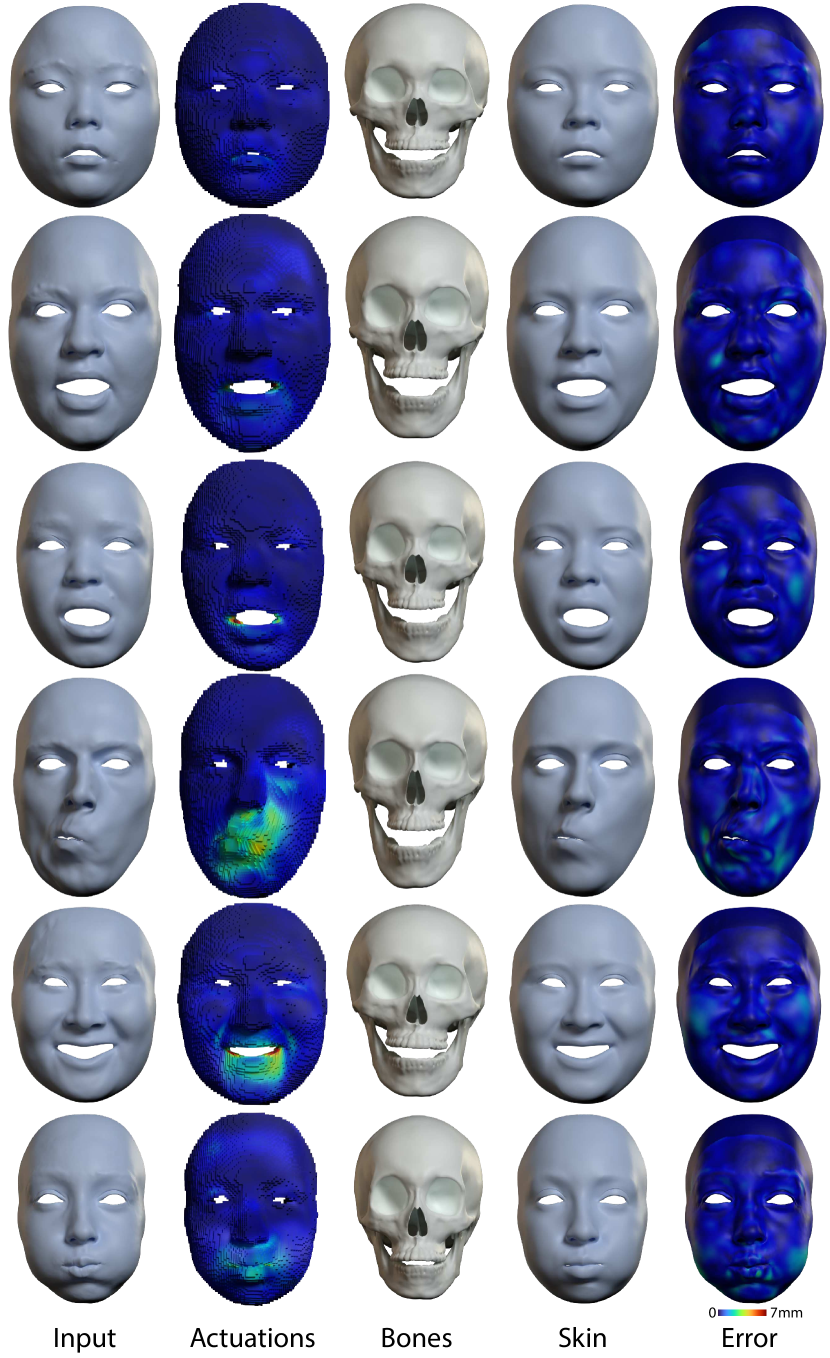
It has become common practice to perform at least a small amount of 3D face scanning for the primary actors in high-end productions. Given just a single scan, our model can be fit to provide physics-based animation. When fitting to a 3D scan, $\mathcal{L}_{\text{skin}}$ and $\mathcal{L}_{\text{bone}}$ are defined the same way as during training (Eqn. (17) and Eqn. (22)). Several fitting results are shown in Fig. 3, including the input scan, the predicted actuations (for the predicted simulation meshes), the estimated bone shapes and mandible transformation, and the final simulated facial skin surface. We highlight the very low error between the simulated result and the input scan. Note that the input scan does not need to be in a rest configuration since we fit both the identity and the expression parameters. In this application, fitting takes less than 15 seconds on a desktop machine with a commodity GPU (Nvidia GTX 1080Ti), yielding an incredibly fast method to obtain an identity-specific physical face model.

Figure 3. Model fitting to a 3D scan. Five examples are shown for different identities and different expressions. After fitting, the predicted actuations and bones allow to simulate the final facial skin mesh, which matches the input with a very low error.

Fitting to a Face Image.

When a 3D scan is not available, our model is flexible and can be fit even to a single face image. When fitting to an image the skin loss is defined in terms of 2D facial landmarks, and our method predicts not only $\beta$ and $\gamma$ but also the camera projection matrix $\mathbf{C}$. $\mathcal{L}_{\text{skin}}$ is then defined as:

(26) $$\mathcal{L}_{\text{skin}}(\partial\Omega_{\text{skin}}^{0})=\sum_{i=1}^{N_{l}}\frac{1}{N_{l}}||\mathbf{C}\cdot\mathcal{N}_{e}(\mathbf{X}_{i})-\hat{\mathbf{x}}_{i}||^{2}_{2},$$

where $\mathbf{X}_{i}$ represents the $i$-th landmark out of the $N_{l}$ landmarks sampled from $\partial\Omega_{\text{skin}}^{0}$, and $\hat{\mathbf{x}}_{i}$ indicates the corresponding ground truth 2D landmark position in screen space. To obtain the ground truth landmarks we employ a recent high-quality dense landmark detector (Chandran et al., 2023) and predict approximately 8000 landmarks distributed on the face (please refer to the supplemental video for an illustration). In this scenario, there is no ground truth neutral scan to obtain a predicted bone shape for the bone shape loss $\mathcal{L}_{\text{bone}}$ in Eqn. (22). However, we can reformulate $\mathcal{L}_{\text{bone}}$ as a self-supervised bone loss using the estimated skin to predict the bones:

(27) $$\mathcal{L}_{\text{bone}}(\partial\Omega_{\text{bones}}^{c})=\sum_{i=1}^{N_{b}}\frac{1}{N_{b}}||\mathcal{N}_{c}(\mathbf{X}^{c}_{i})-\mathcal{P}(\mathcal{N}_{c}(\partial\Omega_{\text{skin}}^{c}))(\mathbf{X}^{c}_{i})||^{2}_{2},$$

where $\mathcal{P}$ represents the SCULPTOR predictor model, evaluated on the regressed neutral facial skin $\mathcal{N}_{c}(\partial\Omega_{\text{skin}}^{c})$. Fitting results are shown in Fig. 1 and Fig. 4. We systematically evaluate a variety of images with differing resolutions and lighting conditions. While not as accurate as fitting to a ground truth 3D scan, the image fitting results showcase our ability to preserve critical facial features while providing the most flexible and easy-to-employ version of our model.

Figure 4. Model fitting to a single face image. Five different identities and expressions are shown. After fitting, the predicted actuations and bones allow to simulate the final facial skin mesh. The result is an animatable physical model from a very lightweight input.

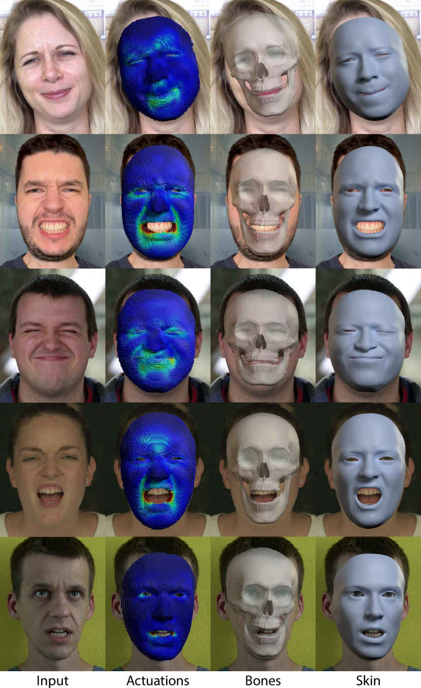
For all fitting results, either to scan or to image, once the parameters are fit then the model can be animated as illustrated in Fig. 1 and the supplemental video.

6.2. Physical Effects

Our model allows the simulation of physical effects, which is one of the key benefits of using physically-based animation.

Figure 5. Collision handling. Our physical model is able to accurately detect and resolve interpenetrating geometries.

Figure 6. Paralysis. Our physical model can simulate some degrees of facial paralysis, demonstrating the model’s sensitivity and precision in depicting subtle physiological changes.

Figure 7. Bone reshaping. Our physical model can simulate various craniofacial effects like osteotomy, where the jaw has been scaled down and the actuations are replayed on the edited anatomy.

Figure 8. Gravity. We show the effect of gravity on a stabilized face with different head orientations (inset).

Collision Handling.

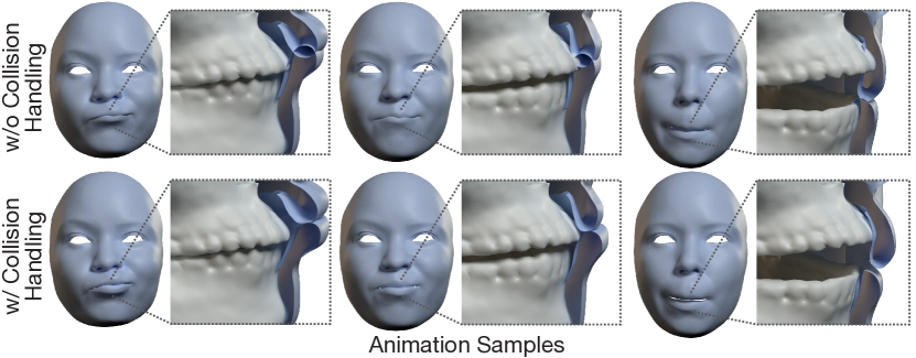
Fig. 5 illustrates our model’s capacity to accurately detect and resolve collisions, including lip-lip and bone-lip penetrations, a common challenge in facial animation.

Paralysis.

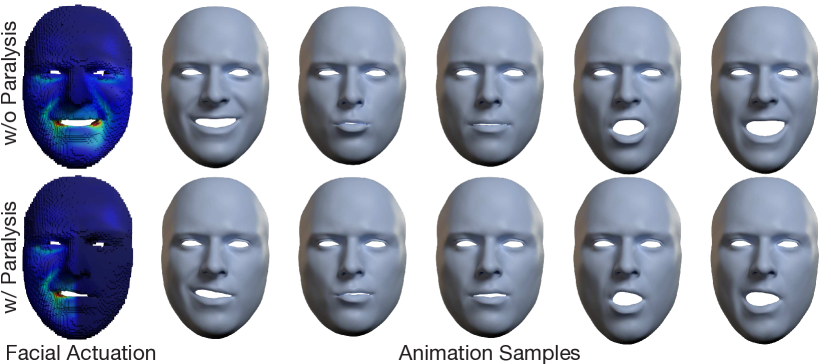
By adjusting muscle actuation parameters, our model can replicate some degrees of facial paralysis as illustrated in Fig. 6. This example demonstrates the model’s sensitivity and precision in depicting subtle physiological changes.

Bone Reshaping.

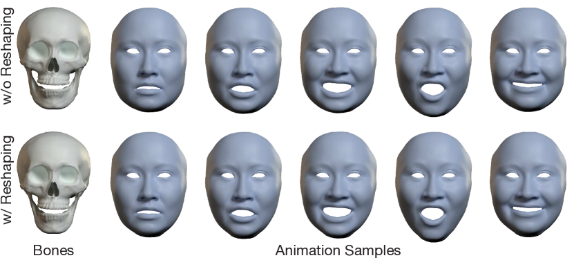
Our physical model can simulate various craniofacial effects like osteotomy, illustrated in Fig. 7 where the jaw bone has been scaled down, showing the comparative analysis between pre- and post-treatment states and highlighting our model’s effectiveness in representing and adapting to skeletal deformations.

Gravity.

Our model can simulate the effects of gravity. Fig. 8 shows this effect where we rotate the head to different orientations and the soft tissue is naturally pulled in the corresponding direction.

6.3. Retargeting

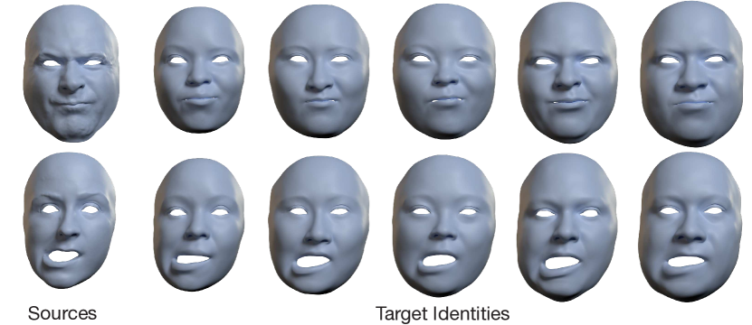
Our model can be used for physics-based animation retargeting, where we transfer facial animations between identities without interpenetration (see Fig. 9). This is accomplished by changing the identity latent code to a target subject while keeping the expression code of the source subject. This application confirms our model’s ability to maintain realism and physical integrity while producing identity-specific facial expressions that match a source input.

6.4. Latent Space Interpolation

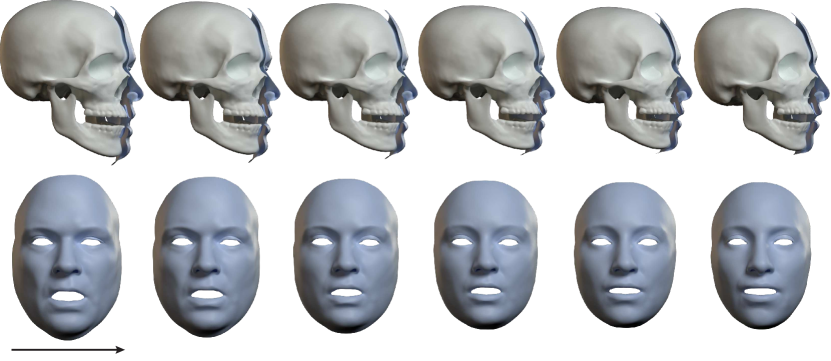
Another application of our generalized model is that we can sample new identities from the latent space. We demonstrate this by interpolating between two different identities from our training set in Fig. 10. For each novel identity, the model can be evaluated with different expression codes to obtain physics-based facial animation.

Figure 9. Our physical model is able to transfer facial animations between different identities while being interpenetration-free.

Figure 10. Our physical model is able to smoothly interpolate between different identities while preserving physical plausibility, such as collision-free properties.

7. Evaluation

We evaluate our model from multiple perspectives numerically, including reconstruction accuracy, jaw rigidity, skull fixation and anatomical fidelity. For reconstruction accuracy, we adopt four types of metrics, including 3D vertex-to-vertex error (V2V), 3D scan-to-mesh error (S2M), F-Score, and normal error. Finally, we evaluate anatomical fidelity in terms of the bone fidelity and the bone-skin penetration. The specific details of each metric are elaborated as follows:

• Vertex-to-vertex Error (V2V) measures the average of the Euclidean distances between the ground-truth and the reconstruction vertices.

• Scan-to-mesh Error (S2M) measures the average of the Euclidean distances between the ground-truth vertices and the reconstructed mesh surface.

• F-Score evaluates the reconstruction quality from the point cloud aspect. It harmonizes the recall and the precision by computing their harmonic mean. A high F-Score is indicative of a reconstruction that is both accurate and complete. We sample 32k points in total and use 1mm as the error threshold.

• Normal Error measures the average of the cosine distances between the ground-truth and the reconstruction normals.

• Jaw Rigidity quantifies how rigidly the network moves the jaw, based on V2V metric (see Eqn. (12)).

• Skull Fixation quantifies how well the network fixes the skull, based on V2V metric (see Eqn. (13)).

• Bone Fidelity quantifies how well the network preserves the SCULPTOR bone space, based on V2V metric (see Eqn. (16)).

• Penetration Pairs counts the penetration between the bone and the skin meshes. We use the edge-triangle pair.

Table 2. Numerical evaluation of different simulation resolutions.

Res. (mm)	V2V $\downarrow$	S2M $\downarrow$	F-Score $\uparrow$	Normal $\downarrow$
$6.8$	1.4679	0.6615	0.7346	0.0178
$4.5$	1.1270	0.5466	0.8033	0.0157
$3.0$	0.9469	0.4892	0.8427	0.0146
$2.0$ (Ours)	0.8975	0.4721	0.8546	0.0143
$1.3$	0.8848	0.4666	0.8583	0.0142
$0$    (Disp)	0.8642	0.4532	0.8672	0.0141

Model Accuracy.

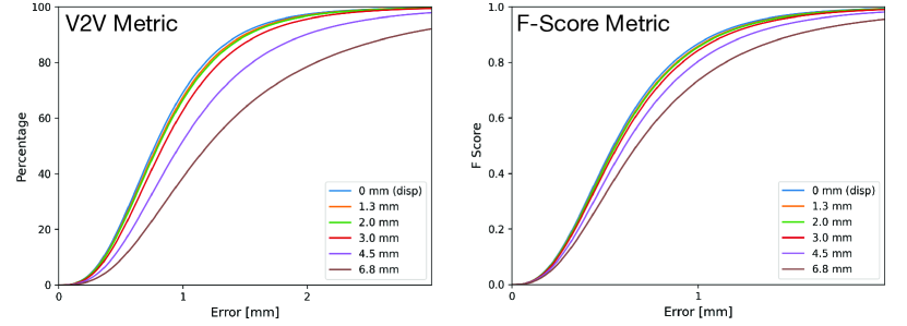
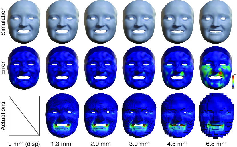
We first evaluate our model accuracy in terms of fitting accuracy. Specifically, we fit our model to the static test set by optimizing our latent codes scan by scan, using $\mathcal{L}_{\text{test}}$ (Eqn. (19)). We then run the discretization and the simulation to get the results for calculating the metrics. Table (2) reports the accuracy of our model with different discretization resolutions. The discretization resolution largely impacts the simulation accuracy. The higher the resolution is, the more accurate the simulated results are. We include a row for evaluating the pure displacement output of the network, labelled “0 (Disp)”, which has the lowest error as this is the target of the training objective. With a discretization resolution of around $2$mm we can achieve comparable accuracy with our displacement outputs, substantiating that our simulation-free learning framework is effective in inferring plausible physical constraints used in simulation. Fig. 11 plots the cumulative curves on V2V and F-Score metrics. Fig. 12 further demonstrates that our simulation results can achieve high reconstruction quality.

Figure 11. Cumulative curves of V2V and F-Score metrics from different simulation resolutions.

To further evaluate our model in terms of animation quality, we test our model on the dynamic set, where we directly use the unseen expression blendweight vectors to animate the seen identities without any optimization. Table (3) shows that the model generalizes well to the unseen expression blendweights, paving the way for animation retargeting. We also report the jaw rigidity and skull fixation in both datasets, proving that the constraints are well enforced (see Table (3)).

Figure 12. Qualitative comparison of different simulation resolutions.

Figure 13. Qualitative comparison of different methods.

Table 3. Numerical evaluation of different components on static and dynamic test sets. We turn on the latent space optimization for static set while turn off it for dynamic set.

	Methods	V2V $\downarrow$	S2M $\downarrow$	F-Score $\uparrow$	Normal $\downarrow$	Jaw Rig. $\downarrow$	Skull Fix.$\downarrow$
Static	Ours w/o $\mathcal{L}_{\text{bone}}$	0.8942	0.4702	0.8560	0.0143	0.1378	0.0724
	Ours w/o $\mathcal{L}_{\text{rigid}}$	1.2891	0.6758	0.7552	0.0158	2.2540	0.1145
	Ours w/o $\mathcal{L}_{\text{soft}}$	0.9282	0.5077	0.8567	0.0158	0.0460	0.0647
	Ours w/o $\mathcal{L}_{\text{lip}}$	0.9178	0.4804	0.8486	0.0144	0.1338	0.0764
	Ours	0.8975	0.4721	0.8546	0.0143	0.1349	0.0785
Dynamic	Ours w/o $\mathcal{L}_{\text{bone}}$	0.7237	0.3182	0.9396	0.0070	0.0883	0.0557
	Ours w/o $\mathcal{L}_{\text{rigid}}$	1.0632	0.4918	0.8407	0.0077	2.1084	0.0866
	Ours w/o $\mathcal{L}_{\text{soft}}$	0.7815	0.3723	0.9059	0.0086	0.0296	0.0400
	Ours w/o $\mathcal{L}_{\text{lip}}$	0.7751	0.3399	0.9270	0.0071	0.0915	0.0612
	Ours	0.7248	0.3235	0.9354	0.0070	0.0915	0.0638

Ablation.

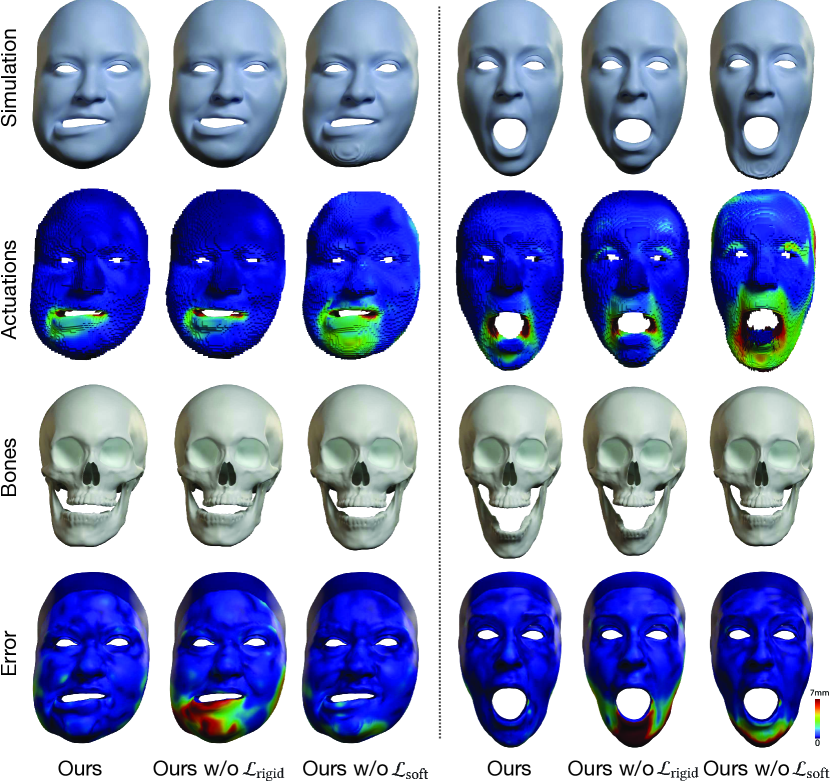
There are two main integral loss terms in our learning framework, the rigidity loss $\mathcal{L}_{\text{rigid}}$ (Eqn. (12)) and the soft loss $\mathcal{L}_{\text{soft}}$ (Eqn. (14)). In Table (3) and Fig. 13, we show the ablation studies of the reconstructions denoted as ”Ours w/o $\mathcal{L}_{\text{rigid}}$” and ”Ours w/o $\mathcal{L}_{\text{soft}}$” to assess the importance of each loss term. For both the quantitative and qualitative measurements, removing one loss term results in a severe performance decrease, which confirms both loss terms contribute to higher reconstruction accuracy and better physical plausibility. Specifically, $\mathcal{L}_{\text{rigid}}$ helps to enforce the rigid movement of the bone, giving better jaw rigidity and skull fixation metrics. This leads to better accuracy since the learned actuation mechanisms are more compatible with the rigid jaw kinematics that are strictly enforced during simulation. $\mathcal{L}_{\text{soft}}$ gives birth to two merits. First, it helps the model learn plausible soft tissue deformation (see Actuations in Fig. 13). Second, it builds the connection between the bone and the skin, therefore being able to gradually drag the jaw to the physically plausible places during training. Therefore, ”Ours w/o $\mathcal{L}_{\text{soft}}$” fails to infer the jaw kinematics and always produces fixed jaw position (see Bones in Fig. 13). This is why its jaw rigidity metrics and skull fixation are better than our full model (Table (3)).

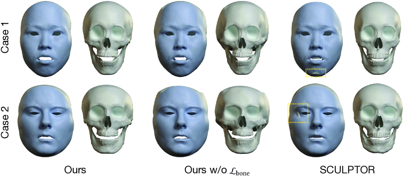
We also examine the effectiveness of our bone shape loss $\mathcal{L}_{\text{bone}}$ by training another model without it, denoted as ”Ours w/o $\mathcal{L}_{\text{bone}}$”. Table (5) and Fig. 15 show that $\mathcal{L}_{\text{bone}}$ can better constrain the overall bone shape. Finally, our Lipschitz regularization $\mathcal{L}_{\text{lip}}$ leads to better reconstruction accuracy without spoiling other metrics (see ”Ours w/o $\mathcal{L}_{\text{lip}}$” vs. ”Ours” in Table (3) and Table (5)).

Figure 14. Qualitative comparison with FLAME. On the left, we show the fitting error maps. On the right, we show the animation samples with the mouth cut-away on the side of each frame.

Figure 15. Qualitative comparison of different methods in terms of anatomy.

Comparison.

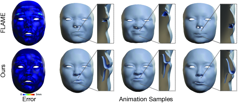
As the first generalized physical face model, we benchmark our method against the closely related FLAME model, focusing on fitting accuracy. Recognizing that FLAME optimizes using scan-to-mesh distance, we adopt the same metric, replacing the vertex-to-vertex energy in our fitting scheme with scan-to-mesh distance, to ensure an equitable comparison. Beyond our static test set, we have compiled an additional test set of comparable size from the FACESCAPE dataset (Yang et al., 2020b). Results presented in Table (4) indicate that our method attains accuracy on par with FLAME across both datasets. A significant advantage of our model, however, lies in its ability to support additional physical effects, such as collision handling—areas where traditional methods often falter. Fig. 14 provides a qualitative comparison to highlight this capability.

In addition, we conduct a comparison of our model with SCULPTOR, specifically focusing on the issue of bone-skin penetration. Our experiments reveal that fitting SCULPTOR to a neutral scan frequently results in bone-skin penetration problems. However, thanks to our elastic regularization ($\mathcal{L}_{\text{ereg}}$), our model effectively mitigates these issues. At the same time, it maintains comparable bone shape (see Fig. 15 and Table (5)).

Finally, our method is still applicable in Yang et al’s scenario when the material space is provided (Yang et al., 2023). To show this, we integrate our unique loss functions—$\mathcal{L}_{\text{skin}}$, $\mathcal{L}_{\text{rigid}}$, and $\mathcal{L}_{\text{fix}}$—into Yang et al.’s model architecture, while still adhering to their established regularization and training protocols. Table (6) shows the evaluation on their test set. Our method not only achieves comparable accuracy, but it also offers significantly improved scalability. For instance, whereas Yang et al. required six GPUs and nearly 2 days to train models for six identities, our methodology can be efficiently implemented on a single GPU, enabling training for over 300 identities in just one day.

Table 4. Scan-to-mesh distance of different models on different datasets.

Datasets	Ours*	FLAME-100	FLAME-300
Our Dataset	0.3487	0.4858	0.4318
FaceScape	0.4713	0.6355	0.5596

Table 5. Anatomical evaluation of different models on neutral scans.

Methods	Penetration Pairs $\downarrow$	Bone Fidelity $\downarrow$
Ours w/o $\mathcal{L}_{\text{bone}}$	0	1.9979
Ours w/o $\mathcal{L}_{\text{lip}}$	0	1.3124
Ours	0	1.3164
Sculptor	2628	0

Table 6. Quantitative Comparison with (Yang et al., 2023).

Metric	Yang et al	Ours
V2V	0.3849	0.3813

8. Conclusion

We present a new model for physics-based facial animation that is trained on real data of hundreds of identities performing various expressions, and as such is extremely generalizable and can be fit to new unseen identities at runtime. As a result, we propose a very convenient way to generate actor-specific physical face animation without any manual model setup. This is possible due to our two main contributions: an approach for simulation-free learning where neural networks are trained to produce deformations that are compatible with physical simulation but without requiring simulation in the training loop, and a material space morphing method that can predict actor-specific skin, bones and soft-tissue volumes automatically. These contributions are the key to being able to train on such a large dataset efficiently, providing the generalizability needed for fitting to new identities.

In terms of limitations, we note that we do not attempt to accurately model the inside of the mouth, in part because the training dataset does not accurately track this region. As such, we ignore the teeth region on the anatomy model. Also, while we endeavor to create constraints that produce physically-accurate animations, there is no guarantee that the learned actuations are biologically accurate, especially for unseen identities that are far from the ones seen at training time.

Nevertheless, we demonstrate the success of our trained model with very plausible applications of fitting to new face scans, fitting to face images, animating with physical effects, animation retargeting and identity interpolation. We additionally provide a detailed evaluation of our method. We hope that our work will help to democratize physics-based facial animation for many applications.