Lifelong Benchmarks: Efficient Model Evaluation in an Era of Rapid Progress

Abstract

Standardized benchmarks drive progress in machine learning. However, with repeated testing, the risk of overfitting grows as algorithms over-exploit benchmark idiosyncrasies. In our work, we seek to mitigate this challenge by compiling ever-expanding large-scale benchmarks called Lifelong Benchmarks. As exemplars of our approach, we create Lifelong-CIFAR10 and Lifelong-ImageNet, containing (for now) 1.69M and 1.98M test samples, respectively. While reducing overfitting, lifelong benchmarks introduce a key challenge: the high cost of evaluating a growing number of models across an ever-expanding sample set. To address this challenge, we also introduce an efficient evaluation framework: Sort & Search (S&S), which reuses previously evaluated models by leveraging dynamic programming algorithms to selectively rank and sub-select test samples, enabling cost-effective lifelong benchmarking. Extensive empirical evaluations across $\sim$31,000 models demonstrate that S&S achieves highly-efficient approximate accuracy measurement, reducing compute cost from 180 GPU days to 5 GPU hours ($\sim$1000x reduction) on a single A100 GPU, with low approximation error. As such, lifelong benchmarks offer a robust, practical solution to the “benchmark exhaustion” problem.

github.com/bethgelab/sort-and-search

github.com/bethgelab/lifelong-benchmarks

1 Introduction

We are in the midst of a benchmark revolution. Datasets like ImageNet (Deng et al., 2009), MS-COCO (Lin et al., 2014), GLUE (Wang et al., 2018) and BigBench (Srivastava et al., 2022) have been instrumental in advancing machine learning research by providing standardised scenarios for comparing models. However, over time, these static benchmarks have been exposed to many evaluations, each leaking cues about their test data and weakening their statistical power as tools of generalisation measurement  (Ott et al., 2022; Mazumder et al., 2023; Kiela et al., 2021). Fresh approaches must compete with a body of methods that have been highly tuned to such benchmarks, incentivising further overfitting if they are to compete (Bender et al., 2021; Beyer et al., 2021). This raises a critical question: What function should such benchmarks serve?

Figure 1: Static vs Lifelong Benchmarking. (Top) Static benchmarks incentivise machine learning practitioners to overfit models to specific datasets, weakening their ability to assess generalisation. (Bottom) We introduce Lifelong Benchmarks as an alternative paradigm—ever-expanding pools of test samples that resist overfitting while retaining computational tractability.

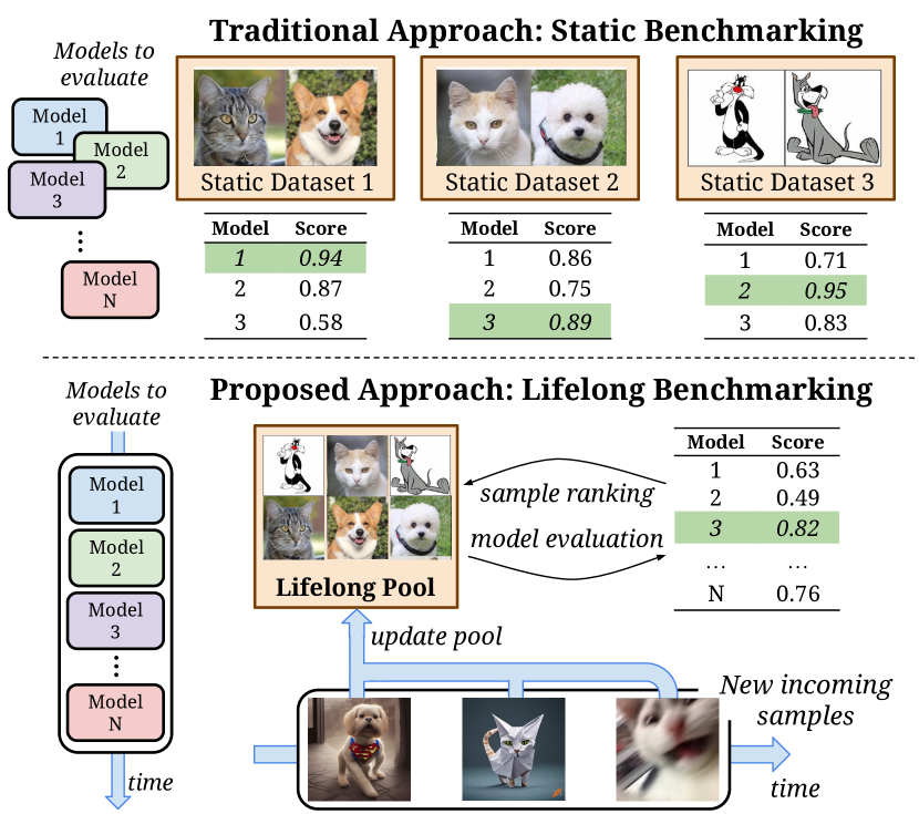
Towards Lifelong Benchmarks. The primary goal of the vision benchmarks considered in this work is to assess model performance on some task using data that is representative of the visual world (Torralba and Efros, 2011). For instance, the CIFAR10 (Krizhevsky et al., 2009) benchmark tested whether classifiers can distinguish between 10 categories, such as dogs and cats. Subsequent versions like CIFAR10.1 (Lu et al., 2020), CIFAR10.2 (Lu et al., 2020), CINIC10 (Darlow et al., 2018), and CIFAR10-W (Sun et al., 2023) introduced more challenging and diverse samples to evaluate the same objective of classifying 10 categories. Over time, however, thanks to repeated evaluation exposure from competing approaches, each individual benchmark diminishes in representativeness as overfitting occurs at both the individual method and research community level (Fang et al., 2023; Vishniakov et al., 2023). In this work, we aim to tackle this challenge by introducing two Lifelong Benchmarks: Lifelong-CIFAR10 and Lifelong-ImageNet. These are ever-expanding pools of test samples that aim to restore the representativeness of benchmarks to the visual world (see Fig. 1) by preventing models from overfitting specifically to the biases of any subset benchmark.

Table 1: Overview of our Lifelong Benchmarks. We list the constituent source datasets (deduplicated) and their statistics for constructing our lifelong benchmarks here. Our benchmarks encompass a wide-range of natural and synthetic domains, sources and distribution shifts, making for a comprehensive lifelong testbed.

Dataset	#Test Samples	#Domains	#Unique Sources	Synthetic/Natural	Corrupted/Clean
Lifelong-CIFAR10	1,697,682	22	9	Both	Both
CIFAR10.1 (Recht et al., 2018)	2,000	1	1	Natural	Clean
CIFAR10 (Krizhevsky et al., 2009)	10,000	1	1	Natural	Clean
CIFAR10.2 (Lu et al., 2020)	12,000	1	1	Natural	Clean
CINIC10 (Darlow et al., 2018)	210,000	1	1	Natural	Clean
CIFAR10-W (Sun et al., 2023)	513,682	3	8	Both	Clean
CIFAR10-C (Hendrycks et al., 2021b)	950,000	19	1	Natural	Corrupted
Lifelong-ImageNet	1,986,310	43	9	Both	Both
ImageNet-A (Hendrycks et al., 2021c)	7,500	1	3	Natural	Clean
ObjectNet (Barbu et al., 2019)	18,514	1	1	Natural	Clean
OpenImagesNet (Kuznetsova et al., 2020)	23,104	1	1	Natural	Clean
ImageNet-V2 (Recht et al., 2019)	30,000	1	1	Natural	Clean
ImageNet-R (Hendrycks et al., 2021a)	30,000	13	1	Natural	Clean
ImageNet (Deng et al., 2009)	50,000	1	1	Natural	Clean
Greyscale-ImageNet (Taori et al., 2020)	50,000	1	1	Natural	Clean
StylizedImageNet (Geirhos et al., 2018)	50,000	1	1	Synthetic	Corrupted
ImageNet-Sketch (Wang et al., 2019b)	50,889	1	1	Natural	Clean
SDNet (Bansal and Grover, 2023)	98,706	19	1	Synthetic	Clean
LaionNet (Shirali and Hardt, 2023)	677,597	1	1	Natural	Clean
ImageNet-C (Hendrycks and Dietterich, 2019)	900,000	19	1	Natural	Corrupted

Evaluation Cost. Our Lifelong-CIFAR10 and Lifelong-ImageNet benchmarks contain 1.69 million and 1.98 million test samples, respectively. A challenge we face with this expanding dataset is the increasing cost of evaluation—it takes roughly 140 and 40 GPU days to evaluate our current model set (containing 31,000 and 167 models respectively, see Section 5.1), on Lifelong-CIFAR10 and Lifelong-ImageNet respectively. Similar issues occur in large-scale foundation model (Bommasani et al., 2021) evaluation. For instance, evaluating a single large language model (LLM) on the MMLU benchmark (Hendrycks et al., 2021b) (standard benchmark for evaluating LLMs) takes 24 hours on a consumer-grade GPU (Ilyas Moutawwakil, 2023). As models grow in complexity, lifelong testing will inevitably lead to a surge in evaluation costs when benchmarking a large set of increasingly expensive models against an ever-growing collection of test samples (Sardana and Frankle, 2023; Dehghani et al., 2021). Can we reduce this evaluation cost while minimising the prediction error?

Efficient Model Evaluation. We develop algorithms for efficient evaluation in lifelong benchmarks by drawing inspiration from the field of computerized adaptive testing (CAT) (Van der Linden and Glas, 2000), which can generate exams like the GRE and SAT from an ever-expanding pool of questions. Unlike traditional tests where all questions must be answered, CAT adaptively sub-samples questions based on examinee responses. This approach efficiently gauges proficiency with far fewer questions, while maintaining assessment accuracy. At the same time, as test takers continue taking the tests, the question pool gets more accurately calibrated, reinforcing this “lifelong testing pool”.

Similarly, in our lifelong benchmarking framework, we aim to evaluate the classification ability of new models without testing them on all samples, instead selecting a subset of samples to evaluate models. We propose a method named Sort & Search (S&S), which reuses past model evaluations on a sample set through dynamic programming to enable efficient evaluation of new, incoming models. S&S operates by first ranking test samples by their difficulty, done efficiently by leveraging data from previous tests. It then uses these updated rankings to evaluate new models, streamlining the benchmarking process. This strategy enables efficient lifelong benchmarking, reducing the cost dramatically from a collective of 180 GPU days to 5 GPU hours on a single A100 GPU. This corresponds to a 1000$\times$ reduction in inference costs compared to static evaluation on all samples. To summarize our key contributions in this work:

1. We introduce and formalise lifelong benchmarking as a novel framework for robust, efficient model evaluation.

2. We curate two lifelong benchmarks: Lifelong-CIFAR10 and Lifelong-ImageNet, consisting of 1.69M and 1.98M samples respectively

3. We propose a novel framework, Sort & Search for efficient model evaluation, reducing over 99.9% of computation costs on our lifelong benchmarks while accurately predicting sample-wise performance.

2 Lifelong Benchmarks: Curation

Considerations. We aim to establish lifelong benchmarking as a standard evaluation protocol in computer vision. To demonstrate this, we considered two popular datasets as our basis: CIFAR10 (Krizhevsky et al., 2009) and ImageNet (Deng et al., 2009). We chose them due to (1) their widespread adoption in prior art, (2) the diverse set of models trained on them, and (3) the presence of numerous dataset variants with the same set of labels, encompassing distribution shifts (Barbu et al., 2019), temporal variations (Shirali and Hardt, 2023), and adversarial samples (Hendrycks et al., 2021c).

Note that while our current lifelong benchmarks are based on two datasets, our framework can generally be applied to any broader range of datasets. We describe the precise construction of our datasets below. See Table 1 for key statistics and a detailed breakdown.

Lifelong-CIFAR10. We combine 22 domains of different CIFAR10-like datasets comprising samples applied with various synthetic distribution shifts, synthetic samples generated by diffusion models, and samples queried from different search engines using different colors and domains. We deduplicate our dataset to ensure uniqueness and downsample all images to the standard CIFAR10 resolution of $32\times 32$. Our final dataset consists of 1.69 million samples.

Lifelong-ImageNet. We source our test samples from ImageNet and its corresponding variants. Similar to Lifelong-CIFAR10, our benchmark is designed for increased sample diversity (43 unique domains) while operating on the same ImageNet class set. We include samples sourced from different web-engines and generated using diffusion models. Our final Lifelong-ImageNet contains 1.98 million samples.

3 Lifelong Benchmarks: Formulation, Challenges and Approach

In this section, we formalise the objective of lifelong benchmarking and describe the key challenges it raises.

Formulation. Let ${\mathcal{D}}{=}{((x_{1},y_{1}),\dots,(x_{n},y_{n}))}$ denote an ordered collection of labelled examples, sampled from the underlying task distribution of interest $P({\mathcal{X}}{\times}{\mathcal{Y}})$. Here, ${x_{i}}{\in}{\mathcal{X}}$ denotes the $i^{\mathrm{th}}$ data sample and ${y_{i}}{\in}{\mathcal{Y}}$ denotes the corresponding label. Let ${\mathcal{M}}{=}{(f_{1},\dots,f_{m})}$ denote an ordered collection of models where each model, ${f}{:}{\mathcal{X}}{\to}{\mathcal{Y}}$, maps data samples to predicted labels. A lifelong benchmark, ${\mathcal{B}}{=}{(\mathcal{D},\mathcal{M},\text{{insert}}_{\mathcal{D}},\text{{insert}}_{\mathcal{M}},\text{{metrics}}}$), augments $\mathcal{D}$ and $\mathcal{M}$ with three operations:
  $\text{{insert}}_{\mathcal{D}}((x^{\prime},y^{\prime}))$ inserts a new labelled example $(x^{\prime},y^{\prime})$ into $\mathcal{D}$.
  $\text{{insert}}_{\mathcal{M}}(f^{\prime})$ inserts a new model $f^{\prime}$ into $\mathcal{M}$.
  $\text{{metrics}}()$ returns a ${|}{\mathcal{M}}{|}$-dimensional vector estimating each model’s performance on the task of interest.

Key challenges. To resist overfitting and provide utility to the research community, we want both the model collection, $\mathcal{M}$, and sample collection, $\mathcal{D}$, to expand over time. To enable this, we can instantiate a “naive” implementation of the $\text{{metrics}}()$ operation ( ) by simply re-evaluating every model on every sample after each call to $\text{{insert}}_{\mathcal{M}}$ ( ) or $\text{{insert}}_{\mathcal{D}}$ ( ). However, such a strategy exhibits $O(|\mathcal{D}||\mathcal{M}|)$ runtime complexity for each call to $\text{{metrics}}()$, rendering benchmark evaluation infeasible as $\mathcal{D}$ and $\mathcal{B}$ grow, hence preventing the practical adoption of the lifelong benchmarking paradigm. The central question considered by this work is therefore the following: Given a lifelong benchmark $\mathcal{B}$, how can we efficiently compute metrics() each time we insert new models into $\mathcal{M}$ ( ) or new labelled samples into $\mathcal{D}$ ( )?

Figure 2: Proposed Lifelong Benchmarking setup. Assume access to an initial pool of $n$ samples and $m$ models that have been evaluated on these samples (left). Our goal is to efficiently evaluate a new model ( $\text{{insert}}_{\mathcal{M}}$) at sub-linear cost (right top) and efficiently insert a new sample into the lifelong benchmark ( $\text{{insert}}_{\mathcal{D}}$) by determining sample difficulty at sub-linear cost (right bottom).

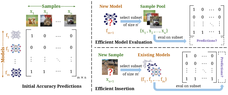
Approach. Our approach is underpinned by two key ideas. First, we augment $\mathcal{B}$ with an instance-level prediction cache to amortise inference costs across evaluations, effectively exchanging (costly) computation for (more affordable) storage (Prabhu et al., 2023). Second, we propose strategies to efficiently populate the cache with new predictions through judicious sampling and inference. The cache is instantiated as a matrix $\mathbf{A}\in\{0,1\}^{|\mathcal{M}|\times|\mathcal{D}|}$ where $\mathbf{A}(i,j)\triangleq\mathbb{I}[f_{i}(x_{j})=y_{j}]$. Given such a cache, metrics() can be computed trivially by row-wise averaging $\mathbf{A}$. Our methodology is illustrated in Fig. 2.

Inserting $\Delta m$ models ( $\text{{insert}}_{\mathcal{M}}$). Suppose that $\Delta m$ new models have been developed after the initial creation of the benchmark. We wish to insert these new models into $\mathcal{M}$ and update the cache accordingly. A naive approach would be to do so by evaluating the $\Delta m$ models on all $|\mathcal{D}|$ samples. Given the high cost of this approach when $|\mathcal{D}|$ grows large, we instead propose to select a small subset of $n^{\prime}\ll|\mathcal{D}|$ samples for evaluation. These are chosen with the goal of enabling accurate prediction of the remaining cache entries.

Inserting $\Delta n$ samples ( $\text{{insert}}_{\mathcal{D}}$). Our second challenge arises when we obtain new $\Delta n$ labelled data examples. We seek to insert these samples into $\mathcal{D}$ and update the cache accordingly. A naive approach entails evaluating all $|\mathcal{M}|$ models on the $\Delta n$ new examples. As above, to substantially reduce cost, we select a small subset of $m^{\prime}\ll|\mathcal{M}|$ models with the objective of accurately predicting the remaining cache entries corresponding to the new $\Delta n$ samples.

Related Work. While the lifelong benchmarking setup introduced has received limited attention, the sub-challenge of efficiently evaluating models has received more focus. Concretely, this maps to the problem of $\text{{insert}}_{\mathcal{M}}$ ( ) within our framework. We comprehensively draw connections across different research directions in the Appendix and briefly present the most similar works here. Model Spider (Zhang et al., 2023) efficiently ranks models from a pre-trained model zoo. LOVM (Zohar et al., 2023) and Flash-HELM (Perlitz et al., 2023) similarly rank foundation models efficiently on unseen datasets. However, these approaches predict dataset-level metrics rather than instance-level metrics, and thereby cannot be used in our setup to grow the prediction cache efficiently.

Concurrent to our work, Anchor Point Sampling (Vivek et al., 2023) and IRT-Clustering (Polo et al., 2024) both propose efficient instance-level evaluations by creating smaller core-sets from test data. They introduce principled methods based on clustering and item response theory (Baker, 2001) to obtain sample-wise accuracy predictions. However, their methods require memory and time complexity of $\mathcal{O}(|\mathcal{D}|^{2})$ with the number of data samples, preventing comparisons on datasets bigger than a few thousand samples. This is infeasible, requiring well over 10TB of RAM, for our lifelong benchmarks having over 1.5 million test samples each. In contrast, our novel Sort & Search approach, requires memory and time complexity of $\mathcal{O}(|\mathcal{D}|\log|\mathcal{D}|)$ with the number of samples, and can scale up to billion-sized test sets (see Section 5 for empirical results).

4 Efficient Benchmarking with Sort & Search

Inspired by the computerized adaptive testing (Van der Linden and Glas, 2000) paradigm, in this section, we propose an efficient evaluation framework for lifelong-benchmarking: Sort & Search (S&S), consisting of two key components: (1) Ranking test samples from the entire dataset pool according to their difficulty, i.e., Sort and (2) Sampling a subset from the pool to predict performance on, i.e., Search. We aim to solve the two key operations that we noted in Section 3 ( $\text{{insert}}_{\mathcal{D}}$ and $\text{{insert}}_{\mathcal{D}}$) with our framework. We now describe the objective and algorithms used in S&S.

4.1 Ranking by Sort

⬇

def sort_by_sum(A):

sum_ranking = A.sum(axis=0)

order = np.flip(np.argsort(sum_ranking))

return order

\pardef two_stage_sort_by_sum(A, idx):

#Step 1: Sum

order = sort_by_sum(A)

#Step 1: Search

thresh = dp_search(A[:, order])

\par#Iterate over bins

bins_ordered = sum_bins[order]

uniq_bins = np.unique(bins_ordered)

\parfor u_bin in uniq_bins:

idx = np.nonzero(bins_ordered==u_bin)[0]

bin_thresh = np.nonzero(np.all([[bins_ordered >= idx.min()], [bins_ordered <= idx.max()]], axis=0))[1]

At = A[thresh][:, order[idx]]

#Step 2: Sum

new_order = sort_by_sum(At)

# Replace current ordering within new in bin

order[idx] = order[idx[new_order]]

return order

Figure 3: Algorithms for Optimizing $\mathbf{P}$ given $\mathbf{Y}$

Setup. We recall that our lifelong benchmark pool consists of evaluations of $|\mathcal{M}|$ models on $|\mathcal{D}|$ samples. For ease of reference, say ${|\mathcal{M}|}{=}{m}$ and ${|\mathcal{D}|}{=}{n}$. For our method, given each model $f_{i}$, $i\in\{1,..,m\}$, we use the binary accuracy prediction per sample, across all $n$ samples obtaining $\mathbf{a}_{i}=[p_{i1},p_{i2}\dots,p_{in}]$. Here, ${p_{ij}}{\in}{\{0,1\}}$ represents whether the model $f_{i}$ classified the sample $x_{j}$ correctly. Thus, for $m$ models and $n$ evaluation samples, we construct a binary matrix $\mathbf{A}\in\{0,1\}^{m\times n}$ by row-wise stacking all the accuracy predictions $\mathbf{a}_{i}$ (see Fig. 2 left).

Goal. Given a data matrix $\mathbf{A}$, we want to obtain a ranked order (from easy to hard) for the columns of $\mathbf{A}$, which represent the samples. This sorted order (Sort) can later be used for efficient prediction on new incoming models (Search). Here, the goal is to find the best global permutation matrix $\mathbf{P}\in\{0,1\}^{n\times n}$, a binary matrix, such that $\mathbf{A}\mathbf{P}$ permutes the columns of $\mathbf{A}$ so that we can rank samples from easy (all 1s across models) to hard (all 0s across all models). We say this has a minimum distance from the optimal ranked accuracy prediction matrix $\mathbf{Y}\in\{0,1\}^{m\times n}$, formally defined as:

$$\mathbf{P^{*}},\mathbf{Y}^{*}=\text{argmin}_{\mathbf{P},\mathbf{Y}}\|\mathbf{A}\mathbf{P}-\mathbf{Y}\|,$$ (1)

$$\textit{s.t. }~{}~{}~{}\mathbf{P}\in\{0,1\}^{n\times n},\mathbf{P}\mathbf{1}_{n}=\mathbf{1}_{n},\mathbf{1}^{\top}_{n}\mathbf{P}=\mathbf{1}_{n},$$

$$\text{if }~{}~{}~{}~{}~{}\mathbf{Y}_{ij}=1\text{, then }\mathbf{Y}_{ij^{\prime}}=1~{}~{}\forall j^{\prime}\leq j,$$

$$\text{if }~{}~{}~{}~{}~{}\mathbf{Y}_{ij}=0\text{, then }\mathbf{Y}_{ij^{\prime}}=0~{}~{}\forall j^{\prime}\geq j.$$

The constraints $\mathbf{P}\mathbf{1}_{n}=\mathbf{1}_{n},\mathbf{1}^{\top}_{n}\mathbf{P}=\mathbf{1}_{n}$ are sufficient to enforce that $\mathbf{P}$ is a permutation matrix. The ranked accuracy prediction matrix $\mathbf{Y}$ is created by a row-wise application of a thresholding operator for every row in $\mathbf{Y}$ separately. Intuitively, if the threshold for the i${}^{\text{th}}$ row is $k$, then the i${}^{\text{th}}$ row is of the form $[\mathbf{1}_{k}^{\top},\mathbf{0}_{n-k}^{\top}]$ where $\mathbf{1}_{k}$ is a vector of all ones of size $k$ and $\mathbf{0}_{n-k}$ is a zero vector of size $n-k$. In every row, all samples before the row-wise threshold $k$ are predicted to be correctly classified (easy) and those after are incorrectly classified (hard) for the model corresponding to the row. The informal explanation of the optimization problem in Equation 1 is to find an ordering of samples such that error introduced by thresholding is minimized.

Given this optimization problem, we next discuss how to solve it. While the goal of this optimization problem is finding the optimal permutation $\mathbf{P}^{*}$, we still need to jointly solve for $\mathbf{P},\mathbf{Y}$ here. We will find a solution by alternating between optimizing $\mathbf{P}$ keeping $\mathbf{Y}$ constant and optimizing $\mathbf{Y}$ keeping $\mathbf{P}$ constant, with the goal of finding the best solution $\mathbf{P}^{*}$, in an EM-style algorithm. We now present algorithms for optimizing the two subproblems in detail.

4.1.1 Optimizing $\mathbf{P}$ given $\mathbf{Y}$

We see from Eq. 1 that $\mathbf{P}$ is binary. This makes finding the optimal $\mathbf{P}^{*}$ an NP-Hard problem (Yuan and Ghanem, 2016). Hence, we discuss how to simplify the sub-problem. We first present an algorithm to solve the case where we can order samples in a strictly decreasing order of difficulty, measured by how many models classified it correctly ( ). However, samples can never be arranged as strictly decreasing in practice. Subsequently, we present one alternative which computes soft confidences, which allows the strictly decreasing constraint to hold ( ). A third alternative algorithm we explore removes the introduced constraint of a strictly decreasing order ( ).

Sorting by Sum. We discuss how to order samples if they follow a strictly decreasing order of difficulty. Formally, considering elements column-wise, the difficulty of each sample (a column) is inversely proportional to the number of $1$s in that column i.e., more $1$s in a column indicates more models classify this sample correctly. We can order samples in decreasing order of difficulty by a simple algorithm detailed in Fig. 3 (sort_by_sum)—intuitively, this algorithm sorts samples from easy (more $1$s) to hard (less $1$s) by sorting the sum vector across rows per column. We call this method Sorting by Sum, which returns an ordering over samples (which can trivially be converted to the permutation matrix $\mathbf{P}^{*}$). However, the assumption of strictly decreasing order of difficulty is unrealistic as the number of samples is usually far larger than the number of models. Hence, it is guaranteed that many samples will have the same level of difficulty by the pigeonhole principle (Ajtai, 1994).

Sorting by Confidence Sum. One method to have a strictly decreasing order is to relax the constraint on the samples of $\mathbf{a}_{i}=[p_{i1},p_{i2}\dots,p_{in}]$ from $p_{ij}\in\{0,1\}$ to $p_{ij}\in[0,1]$, and use confidence of the ground truth class. This modification allows all examples to be unique, allowing Sorting by Sum ( ) to be the best solution, and potentially enable more sample efficient ranking.

⬇

def uniform_sampling(query, num_p):

# idx -> num_p uniformly sampled points

idx = np.arange(0, len(query),

len(query)//num_p)[1:]

return idx

\pardef dp_search(query):

# query is 1 x k (from a row of PA)

# (k can be assigned := n, n’, m, m’)

query[query==0] = -1

cumsum = np.cumsum(query)

idx = np.argmax(cumsum)

return idx/len(query)

# threshold as

Figure 4: Algorithms for Optimizing $\mathbf{Y}$ given $\mathbf{P}$

Recursive Sorting by Sum. Another alternative is relaxing the equal difficulty assumption in Algorithm . A natural question is: How does one order samples which have equal number of models predicting them correctly, i.e., two columns of $\mathbf{A}$ with equal number of $1$s?

We propose an iterative solution: at each step, order samples of equal difficulty by alternatively optimizing $\mathbf{P}$ keeping $\mathbf{Y}$ constant by applying Algorithm and optimizing $\mathbf{Y}$ keeping $\mathbf{P}$ constant by DP-Search algorithm (described next). The recursive aspect is dividing the vector into subsets, where each subset consists of samples which have the same sum. Within each subset, we reorder points by only considering the thresholds obtained when optimizing $\mathbf{Y}$ given $\mathbf{P}$ which fall within this region and recursively applying the alternating minimization. We provide the algorithm for two iterations for an illustration in Fig. 3 (two_stage_sort_by_sum). Note that this strictly improves the solution at each recursion depth. We additionally note that ties are broken by preferring the model which minimizes error the most.

4.1.2 Optimizing $\mathbf{Y}$ given a $\mathbf{P}$

Here, we discuss how to optimize the prediction matrix $\mathbf{Y}$. We re-iterate that we want to find a row-wise threshold $k$ minimizing the error with the matrix $\mathbf{AP}$ for a given permutation $\mathbf{P}$. To optimize $\mathbf{Y}$ given a $\mathbf{P}$, we propose an algorithm based on dynamic programming, called DP-Search, which operates row-wise on each row $\mathbf{y}_{i}$, detailed in Fig. 4 (dp_search). Given a row, it computes the difference between number of $1$s and number of 0s for each index based on a prefix sum structure. Due to the prefix sum structure, for an input of size $n$, the dynamic programming approach reduces the time complexity from quadratic $\mathcal{O}(n^{2}$) to linear $\mathcal{O}(n$). The optimal threshold $k$ is the maximum value in this vector. The vector $\mathbf{y}_{i}$ is simply $[\mathbf{1}_{k}^{\top},\mathbf{0}_{n-k}^{\top}]$ where $\mathbf{1}_{k}$ is a vector of all ones of size $k$ and $\mathbf{0}_{n-k}$ is a zero vector of size $n-k$. DP-Search is guaranteed to return the globally optimal solution, defined as:

Theorem 4.1.

Optimality of $\mathbf{Y}$ given $\mathbf{P}$. For any given $\mathbf{a}_{i}\in\{0,1\}^{1\times n}$ and $\mathbf{P}$, the DP-Search algorithm returns an ordered prediction vector $\mathbf{y}_{i}\in\{0,1\}^{1\times n}$ which is a global minimum of $\|\mathbf{a}_{i}\mathbf{P}-\mathbf{y}_{i}\|_{1}$.

The DP-Search algorithm when applied row-wise independently returns the optimal $\mathbf{Y}$ given $\mathbf{P}$. Now, having optimized the ranking problem, we have a permuation $\mathbf{P}^{*}$ from the data matrix indicating the order of the samples based on difficulty. In the next section we use $\mathbf{P}^{*}$ towards either evaluating new models or adding new samples efficiently.

4.2 Efficient Selection by Search

Given that we have found the best $\mathbf{P}^{*}$ in the sorting phase, we assume this ordering of difficulty of samples generalizes to new incoming models $\Delta m$. Since the problem is separable in each model, it suffices to predict sample-wise accuracies for each new model $f_{m+1}$ on each of the $n$ samples. We will later show that the same pipeline and algorithms work well for the problem of new incoming samples $\Delta n$.

Goal. Given the permutation matrix $\mathbf{P}^{*}$ and $\Delta m$ new models, we want to predict the accuracy across all $n$ samples per model, i.e., predict the accuracy matrix $\mathbf{Y}_{\Delta m}\in\{0,1\}^{\Delta m\times n}$. The primary challenge is to do this by only evaluating on as few samples $n^{\prime}\ll n$ selected per model.

We first restate that the constraints on $\mathbf{Y}$ in Eq. 1 imply a thresholding operator of index from $\{1,\dots,n\}$ for every row in $\mathbf{Y}_{\Delta m}$, i.e., every model in $\Delta m$ independently. Since the problem is separable per row, we consider the problem of optimizing the first new model $\mathbf{y}_{m+1}\in\{0,1\}^{1\times n}$ independently here. Similarly, we denote the corresponding ground truth vector by $\mathbf{a}_{m+1}$, created by evaluating the new model on all $n$ samples, which will be used for evaluating predictions $\mathbf{y}_{m+1}$.

In this section, we answer the two questions. (i) How to find the best-ranked accuracy prediction vector $\mathbf{y}_{m+1}$? (ii) How good is the ranked accuracy prediction vector $\mathbf{y}_{m+1}$?

(i) How to get the optimal $\mathbf{y}_{m+1}$? Our goal here is to generate the sample-wise prediction vector $\mathbf{y}_{m+1}\in\{0,1\}^{1\times n}$. We divide it into two subtasks: selection and optimization. The selection task is to select the best $n^{\prime}$ observations to sample. The optimization task is, given the $n^{\prime}$ observations $\mathbf{a}_{m+1}^{\prime}\in\{0,1\}^{1\times n^{\prime}}$ how to generate the prediction vector $\mathbf{y}_{m+1}\in\{0,1\}^{1\times n}$.

Subtask 1: How to Select Samples? The selection task involves finding the best $n^{\prime}$ observations forming $\mathbf{a^{\prime}}$. We note that any ranked solution we obtain using this array needs to be interpolated from $n^{\prime}$ points to $n$ points, and use this intuition to sample $n^{\prime}$ points. A simple solution is to sample points such that any threshold found minimizes the difference between the actual threshold and a threshold predicted by our set of $n^{\prime}$, i.e., sample $n^{\prime}$ points uniformly, providing the algorithm in Listing 4 (uniform_sampling). We also compare empirically with a pure random sampling approach in Section 5.

Subtask 2: Optimizing $\mathbf{y}_{m+1}$. Here, we discuss that given the $n^{\prime}$ observations $\mathbf{a}_{m+1}^{\prime}\in\{0,1\}^{1\times n^{\prime}}$ how to generate the prediction vector $\mathbf{y}_{m+1}\in\{0,1\}^{1\times n}$. We use the threshold given by the DP-Search (see Listing 4) and obtain the threshold, given in terms of fraction of samples in $|\mathbf{a}_{m+1}^{\prime}|$. We extrapolate this threshold from $n^{\prime}$ to $n$ points, to obtain the threshold for the prediction vector $\mathbf{y}_{m+1}$. The predicted vector $\mathbf{y}_{m+1}$ is simply $[\mathbf{1}_{k}^{\top},\mathbf{0}_{n-k}^{\top}]$ where $\mathbf{1}_{k}$ is a vector of all ones of size $k$ and $\mathbf{0}_{n-k}$ is a zero vector of size $n-k$.

Having studied how to generate the predictions, we next describe how to evaluate them.

(a) Lifelong-CIFAR10

(b) Lifelong-ImageNet

(c) Lifelong-CIFAR10

(d) Lifelong-ImageNet

Figure 5: Main Results. Figure (a,b) We achieve upto 99% cost-savings for doing model evaluation on both Lifelong-ImageNet and Lifelong-CIFAR10 showcasing the efficiency of our Sort&Search method. In Figure (c,d) Power-law fits on the observed absolute-accuracy difference errors ($E_{agg}$) and sampling budget ($n^{\prime}$) relationship reveal large exponents suggesting very quick convergence.

(ii) How good are my predictions? Given a prediction vector $\mathbf{y}_{m+1}$, we can compute the Mean-Absolute Error (MAE), given by $E(\mathbf{a}_{m+1},\mathbf{y}_{m+1})$. It is computed using the Hamming distance to the ground truth vector $\mathbf{a}_{m+1}\in\{0,1\}^{1\times n}$, formally defined as:

$$E(\mathbf{a}_{m+1},\mathbf{y}_{m+1})=\|\mathbf{a}_{m+1}\mathbf{P}^{*}-\mathbf{y}_{m+1}\|_{1}$$ (2)

However, in this section, we want to normalize by the agreement between predictions and ground truth explained by chance alone (refer to Geirhos et al. (2020) for analysis in-depth). We illustrate this with an example where models have 90% accuracy on a binary task with equal number of samples per class. In that case, given two random predictions, 82% of the samples will agree by chance alone. The general metric for agreement between any ground truth vector $\mathbf{a}_{i}$ and a prediction vector $\mathbf{y}_{i}$ by chance is given by:

$$E_{\text{rand}}(\mathbf{a}_{i}, \mathbf{y}_{i})=\frac{\|\mathbf{a}_{i}\|_{1}}{n}\frac{\|\ \mathbf{y}_{i}\|_{1}}{n}$$ (3)

$$+\left(1-\frac{\|\mathbf{a}_{i}\|_{1}}{n}\right)\left(1-\frac{\|\ \mathbf{y}_{i}\|_{1}}{n}\right).$$

The normalized agreement is defined by the Cohen’s Kappa (Cohen, 1960) given as:

$$\kappa(\mathbf{a}_{i},\mathbf{y}_{i})=\frac{(1-E(\mathbf{a}_{i},\mathbf{y}_{i}))-E_{\text{rand}}(\mathbf{a}_{i},\mathbf{y}_{i})}{1-E_{\text{rand}}(\mathbf{a}_{i},\mathbf{y}_{i})}.$$ (4)

where $0\leq\kappa(\mathbf{a}_{i},\mathbf{y}_{i})\leq 1$.

The intuition for this normalization is described in detail in Geirhos et al. (2020). We measure both mean-absolute error (given in Eq. 2) and our defined normalized agreement (given in Eq. 4) as sample-wise metrics in this work. Note that smaller mean-average error $E$ is better but higher normalized agreement $\kappa$ is better.

So far, we have only discussed the efficient evaluation of $\Delta m$ new models ($\leavevmode\hbox to11.77pt{\vbox to11.77pt{\pgfpicture\makeatletter\hbox{\hskip 5.88657pt\lower-5.88657pt\hbox to0.0pt{\pgfsys@beginscope\pgfsys@invoke{ }\definecolor[named]{pgfstrokecolor}{rgb}{0,0,0}\pgfsys@color@gray@stroke{0}\pgfsys@invoke{ }\pgfsys@color@gray@fill{0}\pgfsys@invoke{ }\pgfsys@setlinewidth{0.4pt}\pgfsys@invoke{ }\nullfont\hbox to0.0pt{\pgfsys@beginscope\pgfsys@invoke{ }{ {{}}\hbox{\hbox{{\pgfsys@beginscope\pgfsys@invoke{ }\definecolor[named]{pgffillcolor}{rgb}{0.8,0.13,0.13}\pgfsys@color@rgb@fill{0.8}{0.13}{0.13}\pgfsys@invoke{ }\definecolor[named]{pgfstrokecolor}{rgb}{1,1,1}\pgfsys@color@gray@stroke{1}\pgfsys@invoke{ }\pgfsys@setlinewidth{0.8pt}\pgfsys@invoke{ }{{}{{{}}}{{}}{}{}{}{}{}{}{}{}{}{{\pgfsys@beginscope\pgfsys@invoke{ }\pgfsys@beginscope\pgfsys@invoke{ }\pgfsys@stroke@opacity{0.5}\pgfsys@invoke{ }\pgfsys@fill@opacity{0.5}\pgfsys@invoke{ }\definecolor{pgffillcolor}{rgb}{0.5,0.5,0.5}\pgfsys@color@gray@fill{0.5}\pgfsys@invoke{ }{{ {}{}{}{}{}}{}{{}}{{}}{{}}{{}}\pgfsys@transformcm{1.0}{0.0}{0.0}{1.0}{0.86111pt}{-0.86111pt}\pgfsys@invoke{ }}\pgfsys@moveto{5.48657pt}{0.0pt}\pgfsys@curveto{5.48657pt}{3.03018pt}{3.03018pt}{5.48657pt}{0.0pt}{5.48657pt}\pgfsys@curveto{-3.03018pt}{5.48657pt}{-5.48657pt}{3.03018pt}{-5.48657pt}{0.0pt}\pgfsys@curveto{-5.48657pt}{-3.03018pt}{-3.03018pt}{-5.48657pt}{0.0pt}{-5.48657pt}\pgfsys@curveto{3.03018pt}{-5.48657pt}{5.48657pt}{-3.03018pt}{5.48657pt}{0.0pt}\pgfsys@closepath\pgfsys@moveto{0.0pt}{0.0pt}\pgfsys@fill\pgfsys@invoke{ } \pgfsys@invoke{\lxSVG@closescope }\pgfsys@endscope\pgfsys@invoke{\lxSVG@closescope }\pgfsys@endscope}\pgfsys@beginscope\pgfsys@invoke{ }\definecolor[named]{pgffillcolor}{rgb}{0.8,0.13,0.13}\pgfsys@color@rgb@fill{0.8}{0.13}{0.13}\pgfsys@invoke{ }\definecolor[named]{pgfstrokecolor}{rgb}{1,1,1}\pgfsys@color@gray@stroke{1}\pgfsys@invoke{ }\pgfsys@setlinewidth{0.8pt}\pgfsys@invoke{ }{}\pgfsys@moveto{5.48657pt}{0.0pt}\pgfsys@curveto{5.48657pt}{3.03018pt}{3.03018pt}{5.48657pt}{0.0pt}{5.48657pt}\pgfsys@curveto{-3.03018pt}{5.48657pt}{-5.48657pt}{3.03018pt}{-5.48657pt}{0.0pt}\pgfsys@curveto{-5.48657pt}{-3.03018pt}{-3.03018pt}{-5.48657pt}{0.0pt}{-5.48657pt}\pgfsys@curveto{3.03018pt}{-5.48657pt}{5.48657pt}{-3.03018pt}{5.48657pt}{0.0pt}\pgfsys@closepath\pgfsys@moveto{0.0pt}{0.0pt}\pgfsys@fillstroke\pgfsys@invoke{ } \pgfsys@invoke{\lxSVG@closescope }\pgfsys@endscope}{{{{}}\pgfsys@beginscope\pgfsys@invoke{ }\pgfsys@transformcm{1.0}{0.0}{0.0}{1.0}{-2.5pt}{-3.22221pt}\pgfsys@invoke{ }\hbox{{\definecolor[named]{pgfstrokecolor}{rgb}{0,0,0}\pgfsys@color@gray@stroke{0}\pgfsys@invoke{ }\pgfsys@color@gray@fill{0}\pgfsys@invoke{ }\hbox{{{\color[rgb]{1,1,1}\definecolor[named]{pgfstrokecolor}{rgb}{1,1,1}\pgfsys@color@gray@stroke{1}\pgfsys@color@gray@fill{1}2}}} }}\pgfsys@invoke{\lxSVG@closescope }\pgfsys@endscope}}} \pgfsys@invoke{\lxSVG@closescope }\pgfsys@endscope}}} } \pgfsys@invoke{\lxSVG@closescope }\pgfsys@endscope{{{}}}{}{}\hss}\pgfsys@discardpath\pgfsys@invoke{\lxSVG@closescope }\pgfsys@endscope\hss}}\lxSVG@closescope\endpgfpicture}}\,\text{{insert}}_{\mathcal{M}}$). How do we approach the problem when we want to efficiently extend the benchmark, adding $\Delta n$ new samples ($\leavevmode\hbox to11.77pt{\vbox to11.77pt{\pgfpicture\makeatletter\hbox{\hskip 5.88657pt\lower-5.88657pt\hbox to0.0pt{\pgfsys@beginscope\pgfsys@invoke{ }\definecolor[named]{pgfstrokecolor}{rgb}{0,0,0}\pgfsys@color@gray@stroke{0}\pgfsys@invoke{ }\pgfsys@color@gray@fill{0}\pgfsys@invoke{ }\pgfsys@setlinewidth{0.4pt}\pgfsys@invoke{ }\nullfont\hbox to0.0pt{\pgfsys@beginscope\pgfsys@invoke{ }{ {{}}\hbox{\hbox{{\pgfsys@beginscope\pgfsys@invoke{ }\definecolor[named]{pgffillcolor}{rgb}{0.8,0.13,0.13}\pgfsys@color@rgb@fill{0.8}{0.13}{0.13}\pgfsys@invoke{ }\definecolor[named]{pgfstrokecolor}{rgb}{1,1,1}\pgfsys@color@gray@stroke{1}\pgfsys@invoke{ }\pgfsys@setlinewidth{0.8pt}\pgfsys@invoke{ }{{}{{{}}}{{}}{}{}{}{}{}{}{}{}{}{{\pgfsys@beginscope\pgfsys@invoke{ }\pgfsys@beginscope\pgfsys@invoke{ }\pgfsys@stroke@opacity{0.5}\pgfsys@invoke{ }\pgfsys@fill@opacity{0.5}\pgfsys@invoke{ }\definecolor{pgffillcolor}{rgb}{0.5,0.5,0.5}\pgfsys@color@gray@fill{0.5}\pgfsys@invoke{ }{{ {}{}{}{}{}}{}{{}}{{}}{{}}{{}}\pgfsys@transformcm{1.0}{0.0}{0.0}{1.0}{0.86111pt}{-0.86111pt}\pgfsys@invoke{ }}\pgfsys@moveto{5.48657pt}{0.0pt}\pgfsys@curveto{5.48657pt}{3.03018pt}{3.03018pt}{5.48657pt}{0.0pt}{5.48657pt}\pgfsys@curveto{-3.03018pt}{5.48657pt}{-5.48657pt}{3.03018pt}{-5.48657pt}{0.0pt}\pgfsys@curveto{-5.48657pt}{-3.03018pt}{-3.03018pt}{-5.48657pt}{0.0pt}{-5.48657pt}\pgfsys@curveto{3.03018pt}{-5.48657pt}{5.48657pt}{-3.03018pt}{5.48657pt}{0.0pt}\pgfsys@closepath\pgfsys@moveto{0.0pt}{0.0pt}\pgfsys@fill\pgfsys@invoke{ } \pgfsys@invoke{\lxSVG@closescope }\pgfsys@endscope\pgfsys@invoke{\lxSVG@closescope }\pgfsys@endscope}\pgfsys@beginscope\pgfsys@invoke{ }\definecolor[named]{pgffillcolor}{rgb}{0.8,0.13,0.13}\pgfsys@color@rgb@fill{0.8}{0.13}{0.13}\pgfsys@invoke{ }\definecolor[named]{pgfstrokecolor}{rgb}{1,1,1}\pgfsys@color@gray@stroke{1}\pgfsys@invoke{ }\pgfsys@setlinewidth{0.8pt}\pgfsys@invoke{ }{}\pgfsys@moveto{5.48657pt}{0.0pt}\pgfsys@curveto{5.48657pt}{3.03018pt}{3.03018pt}{5.48657pt}{0.0pt}{5.48657pt}\pgfsys@curveto{-3.03018pt}{5.48657pt}{-5.48657pt}{3.03018pt}{-5.48657pt}{0.0pt}\pgfsys@curveto{-5.48657pt}{-3.03018pt}{-3.03018pt}{-5.48657pt}{0.0pt}{-5.48657pt}\pgfsys@curveto{3.03018pt}{-5.48657pt}{5.48657pt}{-3.03018pt}{5.48657pt}{0.0pt}\pgfsys@closepath\pgfsys@moveto{0.0pt}{0.0pt}\pgfsys@fillstroke\pgfsys@invoke{ } \pgfsys@invoke{\lxSVG@closescope }\pgfsys@endscope}{{{{}}\pgfsys@beginscope\pgfsys@invoke{ }\pgfsys@transformcm{1.0}{0.0}{0.0}{1.0}{-2.5pt}{-3.22221pt}\pgfsys@invoke{ }\hbox{{\definecolor[named]{pgfstrokecolor}{rgb}{0,0,0}\pgfsys@color@gray@stroke{0}\pgfsys@invoke{ }\pgfsys@color@gray@fill{0}\pgfsys@invoke{ }\hbox{{{\color[rgb]{1,1,1}\definecolor[named]{pgfstrokecolor}{rgb}{1,1,1}\pgfsys@color@gray@stroke{1}\pgfsys@color@gray@fill{1}1}}} }}\pgfsys@invoke{\lxSVG@closescope }\pgfsys@endscope}}} \pgfsys@invoke{\lxSVG@closescope }\pgfsys@endscope}}} } \pgfsys@invoke{\lxSVG@closescope }\pgfsys@endscope{{{}}}{}{}\hss}\pgfsys@discardpath\pgfsys@invoke{\lxSVG@closescope }\pgfsys@endscope\hss}}\lxSVG@closescope\endpgfpicture}}\,\text{{insert}}_{\mathcal{D}}$)?

4.3 Efficient Insertion of New Samples ($\text{{insert}}_{\mathcal{D}}$)

To add new samples into our lifelong benchmark efficiently, we have to estimate their “difficulty” with respect to the other samples in the benchmark. To efficiently determine difficulty by only evaluating $m^{\prime}\ll m$ models, a ranking over models is required to enable optimally sub-sampling a subset of $m^{\prime}$ models. This problem is quite similar in structure to the previously discussed addition of new models, where we had to evaluate using a subset of $n^{\prime}\ll n$ samples. How do we connect the two problems?

We recast the same optimization objectives as described in Eq. 1, but replace $\mathbf{A}$ with $\mathbf{A}^{\top}$ and $\mathbf{Y}$ with $\mathbf{Y}^{\top}$. In this case, Eq. 1 would have $\mathbf{A}^{\top}\mathbf{P}$, which would sort models, instead of samples, based on their aggregate sum over samples (i.e., accuracy) optimized using Algorithm to obtain $\mathbf{P}^{*}$, ordering the models from classifying least samples correctly to most samples correctly. Here, Algorithm is sufficient, without needing to solve the joint optimization ( ) because accuracies (sum across rows) are unique as the number of samples is typically much larger than the number of models.

In case of new incoming samples $\Delta n$, we similarly would treat every sample independently and optimize the predicted array $\mathbf{y}^{\top}_{n+1}$ using Efficient Selection by Search (Section 4.2).

5 Experiments

To demonstrate our framework empirically, we showcase experiments on our two tasks: efficient estimation of new sample difficulties ($\text{{insert}}_{\mathcal{D}}$) and efficient performance evaluation of new models ($\text{{insert}}_{\mathcal{M}}$). We then provide a comprehensive analysis of various design choices within our Sort & Search framework.

Figure 6: Estimated v/s Ground-Truth accuracies. For different sampling budgets (${n^{\prime}}{=}{64}{-}{1024}$), our estimated accuracies for $117$ models (Lifelong-ImageNet) and $25,250$ models (Lifelong-CIFAR10) are surprisingly close to ground-truth accuracies (${\rho}{=}{0.86}{-}{0.97}$).

5.1 Experimental Details

Model Space. For Lifelong-CIFAR10, we use $31,250$ CIFAR-10 pre-trained models from the NATS-Bench-Topology-search space (Dong et al., 2021). For Lifelong-ImageNet, we use $167$ ImageNet-1K and ImageNet-21K pre-trained models, sourced primarily from timm (Wightman, 2019) and imagenet-testbed (Taori et al., 2020).

Sample Addition Split ( $\text{{insert}}_{\mathcal{D}}$). To study efficient estimation of new sample difficulties on Lifelong-CIFAR10, we hold-out CIFAR-10W (Sun et al., 2023) samples for evaluation (${\sim}{500,000}$ samples) and use the rest ${\sim}{1.2}$ million samples for sorting. We do not perform experiments on this problem for Lifelong-Imagenet—since the number of models is quite small (167 in total), directly evaluating all models is relatively efficient, as opposed to the more challenging Lifelong-CIFAR10 scenario where evaluation on $31,250$ models is expensive and it is practically possible to reduce the number of models evaluated per new sample.

Model Evaluation Split ( $\text{{insert}}_{\mathcal{M}}$). To study efficient evaluation of new models, we split the model set for the Lifelong-CIFAR10 benchmark into a randomly selected subset of $6,000$ models for ordering the samples (i.e., Sort) and evaluate metrics on the remaining $25,250$ models (i.e., Search). For Lifelong-Imagenet, we use $50$ randomly selected models for ordering the samples (i.e., Sort) and evaluate on $117$ models (i.e., Search).

Metrics ( $\text{{metrics}}()$). We measure errors between estimated predictions for each new model $\mathbf{y}_{m+1}$ and ground-truth predictions $\mathbf{a}_{m+1}$ independently using both instance-level metrics and dataset-level metrics. For instance-level predictions, we measure the mean-average error $E(\mathbf{a}_{m+1},\mathbf{y}_{m+1})$ using Eq. 2 along with the normalized agreement $\kappa$ using Eq. 4. For dataset-level metrics, we measure the absolute difference between estimated and ground truth accuracies, $E_{\text{agg}}=\nicefrac{{\lvert\left(|\mathbf{y}_{m+1}|-|\mathbf{a}_{m+1}|\right)\rvert}}{{n}}$. This gives us a global metric that does not take into account individual sample-level correspondences between $\mathbf{y}_{m+1}$ and $\mathbf{a}_{m+1}$, but rather simply the difference between the aggregate sum of correct predictions.

5.2 Model Performance Estimation ( $\text{{insert}}_{\mathcal{M}}$)

In this set of experiments, we evaluate the predictive power of S&S for evaluating new models ( ) when subjected to a varying number of sampling budgets $n^{\prime}$ i.e., we run our S&S framework over $13$ different sampling budgets: {8, 16, 32, 64, 128, 256, 512, 1024, 2048, 4096, 8192, 16384, 32768} on both Lifelong-ImageNet and Lifelong-CIFAR10.

(a) Sample Difficulty Estimation

(b) Analysis: #Ranking models

(c) Analysis: Ranking methods

(d) Analysis: Sampling methods

Figure 7: Additional Analyses. Figure (a) We achieve accurate sample difficulty estimates on Lifelong-CIFAR10 ($<$0.15 MAE) at a fraction of the total number of models to be evaluated, thereby enabling an efficient insertion of new samples into the ordered set of samples in the benchmark. In Figures (b,c,d), we analyse three design choice axes for a better understanding of the S&S method using the Lifelong-Imagenet dataset.

Figure 8: Error Decomposition Analysis on Lifelong-CIFAR10 (left) and Lifelong-ImageNet (right). We observe that epistemic error (solid line) drops to 0 within only 100 to 1000 samples across both datasets, indicating this error cannot be reduced further by better sampling methods. The total error $E$ is almost entirely irreducible (Aleatoric), induced because new models do not perfectly align with the ranking order $\mathbf{P}^{*}$. This suggests generalizing beyond a single rank ordering, not better sampling strategies, should be the focus of subsequent research efforts.

Unless otherwise specified, our main results in Sections 5.2 and 5.3 use the simple Sorting by Sum algorithm ( , Fig. 3) for obtaining $\mathbf{P}^{*}$ and uniform sampling for the sample budget $n^{\prime}$. We analyze and ablate the other design choices in Section 5.4. We now present our main results.

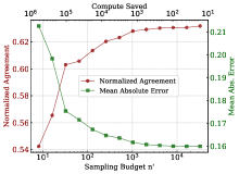
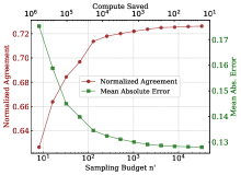
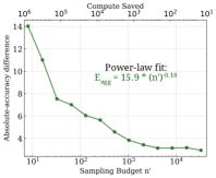
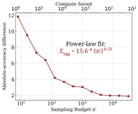
Key Result 1: Extreme Cost-Efficiency. From Figs. 5(a) and 5(b), we observe that our approach converges to a very high normalized agreement and low mean-absolute error with $\nicefrac{{1}}{{1000}}$ the number of evaluation samples, leading to extreme cost savings at inference time (from 180 GPU days to 5 GPU hours on a single A100-80GB GPU). This consistently holds across both datasets on all three metrics: Normalized Agreement, Mean Absolute Error, and Absolute-accuracy difference.

Key Result 2: Prediction Error Scales as a Power-Law. We further analyse the observed $E_{agg}$ against the sampling budget ($n^{\prime}$) relationship by fitting power-laws in Figs. 5(c) and 5(d). The power-laws take the form ${E_{agg}}{=}c{n^{\prime}}^{p}$, where $c$ is the scaling width and $p$ is the exponential coefficient. We find that the power-laws have large exponential coefficients, ${p}{=}{-0.18}$ for Lifelong-CIFAR10 and ${p}{=}{-0.23}$ for Lifelong-ImageNet. This further demonstrates the surprisingly high sample-efficiency obtained by Sort & Search (S&S).

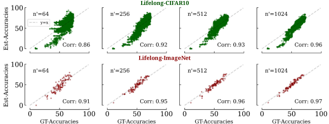
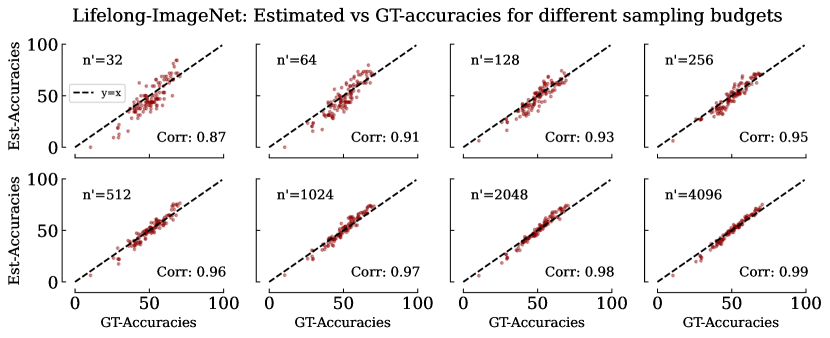
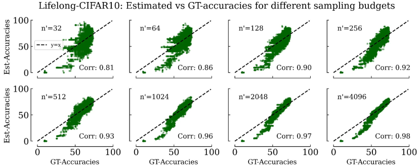
Key Result 3: Highly Accurate Performance Estimation. We note from Fig. 6 that S&S is able to very accurately predict the ground-truth accuracies of models. At a sampling budget ($n^{\prime}$) of just $512$ or $1,024$ samples, our predicted accuracies almost exactly match the true accuracies, as measured by the pearson correlations ($0.96$ for Lifelong-CIFAR10 and $0.97$ for Lifelong-ImageNet at a sampling budget of $1,024$). Note that this performance prediction ability is especially surprising given these results are aggregated over 25,250 models for Lifelong-CIFAR10 and 117 models for Lifelong-ImageNet, spanning a wide range of architectures, model sizes, and accuracies. Additional plots across a more finer variation of $n^{\prime}$ are provided in the Appendix.

5.3 Sample Difficulty Estimation ($\text{{insert}}_{\mathcal{D}}$)

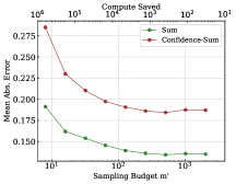
We next showcase results with the complementary task ( ) where for new samples, the goal is to sub-sample the number of models to evaluate on the new samples, for accurately determining sample difficulty. We present results on this task on the Lifelong-CIFAR10 benchmark with two different methods for ranking models, Sorting by Sum ( ) and Sorting by Confidence Sum ( ). We evaluate over different model budgets $m^{\prime}$ (the number of models we use to evaluate our samples over): $\{8,16,32,64,128,256,512,1024,2048\}$. From Fig. 7(a), we observe that both methods converge quickly—Sorting by Sum ( ) reaches a mean-absolute error of less than 0.15 by only evaluating on ${m^{\prime}}{=}{64}$ models out of $31,250$ ($10^{4}\times$ computation savings). This demonstrates our method’s ability to efficiently determine sample difficulty, enabling efficient insertion back into the lifelong-benchmark pool.

5.4 Breaking down Sort & Search

We next nalyse the different design choices used in our S&S framework, and compare their induced efficiency gains.

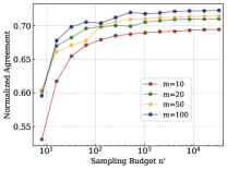
Varying the Number of Models Used for Ranking. In Fig. 7(b), we analyse the effect of the number of models used for computing the initial ranking (i.e., $m$) on the final performance prediction on Lifelong-ImageNet. Having access to more models seems to be a key factor in improving prediction accuracy since using a lower number of models for ranking (${m}{=}{10}$) converges to a smaller normalised agreement (4% performance difference at convergence when using ${m}{=}{100}$ (blue line) compared to ${m}{=}{10}$ (red line)). Interestingly, the number of models $m$ used for ranking does not have any effect on the speed of convergence itself (all methods roughly converge at the same sampling budget (${n^{\prime}}{=}{2,048}$)), but rather only on the prediction accuracy.

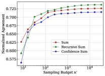
Different Sorting Methods. We compare the three different algorithms on Lifelong-Imagenet: Sorting by Sum, Sorting by Confidence Sum, and Sorting by Recursive Sum. From Fig. 7(c), we note no substantial benefits to using the continual relaxation of the accuracy prediction values as confidence values, in fact, this degrades the predictive accuracy of our method. However, using the multi-step recursive correction of rankings ( ) provides significant boosts (2% boost in normalized agreement at all ${n^{\prime}}{>}1,024$) due to its ability to locally correct ranking errors that the global sum method ( ) is unable to account for.

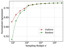
Different Sampling Methods. In Fig. 7(d), we compare the method used for sub-selecting the data-samples to evaluate—we compare between uniform and random sampling. Both methods converge very quickly and at similar budgets to their optimal values and start plateauing. Worth noting however is that uniform sampling provides large boosts over random sampling when the sampling budget is small (10% better in absolute normalized agreement at ${n^{\prime}}{=}{8}$)—this can be attributed to its “diversity-seeking” behaviour which helps cover samples from all difficulty ranges and hence better represent the entire benchmark evaluation samples than an unrepresentative random set that is sampled from the random sampling approach.

6 Decomposing the Errors of S&S

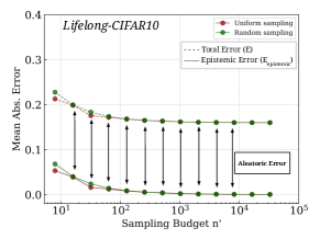
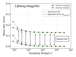
In this section, we showcase that the errors of Sort & Search can be intuitively decomposed. The total mean absolute error $E(\mathbf{a}_{m+1},\mathbf{y}_{m+1})$ can be decomposed into a component irreducible by further sampling, referred to as the Aleatoric Sampling Error ($E_{\text{aleatoric}}$), and a component which can be improved by querying larger fraction of samples $n^{\prime}$, referred to as the Epistemic Sampling Error ($E_{\text{epistemic}}$).

Aleatoric Sampling Error. Let $\mathbf{y}_{m+1}^{*}=\mathbf{y}^{\prime}$ when $n^{\prime}=n$, i.e., it is the best prediction obtainable across all subsampled thresholds, as we have access to the full $\mathbf{a}_{m+1}$ vector. However, some error remains between $\mathbf{y}^{*}$ and $\mathbf{a}_{m+1}$ due to the ordering operation (i.e., Sort). This error, caused by errors in the generalization of the permutation matrix $\mathbf{P}^{*}$ cannot be reduced by increasing the sample budget $n^{\prime}$. More formally, we define this error as:

$$E_{\text{aleatoric}}(\mathbf{a}_{m+1},\mathbf{y}_{m+1}) =\min_{\mathbf{y}_{m+1}}\|\mathbf{a}_{m+1}\mathbf{P}^{*}-\mathbf{y}_{m+1}\|$$ (5)

$$=\|\mathbf{a}_{m+1}\mathbf{P}^{*}-\mathbf{y}_{m+1}^{*}\|.$$

Epistemic Sampling Error. On the contrary, there is a gap between the optimal ranking prediction $\mathbf{y}_{m+1}^{*}$ and $\mathbf{y}_{m+1}$ with the current sample size $n^{\prime}$. This gap, referred to as Epistemic Sampling Error is formally defined as:

$$E_{\text{epistemic}}(\mathbf{y}_{m+1}^{*},\mathbf{y}_{m+1})=\|\mathbf{y}_{m+1}^{*}-\mathbf{y}_{m+1}\|.\\$$ (6)

Note that in a similar way, we can also decompose the normalized agreement metric $\kappa$ simply by computing $\kappa_{\text{aleatoric}}(\mathbf{a}_{m+1},\mathbf{y}_{m+1})=\kappa(\mathbf{a}_{m+1},\mathbf{y}_{m+1}^{*})$ and $\kappa_{\text{epistemic}}(\mathbf{y}_{m+1}^{*},\mathbf{y}_{m+1})=\kappa(\mathbf{y}_{m+1}^{*},\mathbf{y}_{m+1})$.

Results. We analyse the effectiveness of sampling in Lifelong CIFAR-10 and Lifelong-ImageNet by studying the Epistemic Sampling Error ($E_{\text{epistemic}}$) and Aleatoric Sampling Error ($E_{\text{aleatoric}}$) in Figure 8. First, we see that the epistemic error is very low and quickly converges to 0, i.e., we converge to the best achievable performance within sampling just 100 to 1000 samples on both datasets. The remaining error after that is irreducible, and is primarily caused by generalization gaps in the permutation matrix $\mathbf{P}^{*}$. Further, we note that the Recursive Sum algorithm ( ) does not help reduce the gap as shown in Fig. 7(c). This gap is attributable to new models inherently not following a single ranking order across all samples.

7 Open Problems

Although showcasing very promising results in enhancing the efficiency of evaluating Lifelong Benchmarks, our investigation with S&S leads to some interesting open problems:

(1) One-Step Process: Currently, our approach is restricted to one-step sample ranking and model evaluation, whereas ideal lifelong evaluation would need simultaneous optimization of these steps. How do we extend our framework to multi-step continual ranking and evaluation?

(2) Ranking Imprecision: Our error decomposition analysis provides convincing evidence (Section 6) that the ordering of samples $\mathbf{P}^{*}$ while evaluating new models bottlenecks prediction performance. Generalizing from imposing a single sample ordering $\mathbf{P}^{*}$ to sample ordering structures, such as different clusters of models each with their own orderings or rejection frameworks for models if it does not align with the ordering could dramatically improve the framework.

(3) Identifying Difficult Samples: Finding and labeling challenging examples is an essential task for lifelong benchmarks, which is not the focus of our work. Studying hard or adversarial sample selection approaches with lifelong benchmarking is a promising direction. We provide an extensive survey of related approaches in this direction in the Appendix.

8 Conclusion

In this work, we introduced Lifelong-Benchmarks: a framework for dynamically expanding a pool of test samples, designed to enhance the robustness of current benchmarks by mitigating the issue of overfitting to specific dataset biases. As two instances of this paradigm, we curated Lifelong-CIFAR-10 and Lifelong-ImageNet containing over a million evaluation samples each. To counter the challenge of increasing evaluation costs on such large-scale benchmarks, we proposed an efficient framework called Sort & Search that leverages previous model predictions to rank and selectively evaluate test samples. Our extensive experiments, involving over 30,000 models, demonstrate that our method reduces over 99% of evaluation costs. We hope our Lifelong Benchmarking strategy spurs more robust and efficient evaluations.

9 Correlation plots between estimated and ground-truth accuracies

In this section, we expand Fig. 5(d) from the main paper with more datapoints.

Figure 9: Estimated v/s Ground-Truth accuracies on Lifelong-ImageNet. For different sampling budgets($n^{\prime}=32-4096$), our estimated accuracies for 117 models are surprisingly close to the true ground-truth accuracies ($\rho=0.94-1.0$).

Figure 10: Estimated v/s Ground-Truth accuracies on Lifelong-CIFAR10. For different sampling budgets ($n^{\prime}=32-4096$), our estimated accuracies for 25,250 models are surprisingly close to the true ground-truth accuracies ($\rho=0.81-0.98$).

10 Extended Related Work

In this section, we expand on the brief literature review from Section 3 for a more expansive coverage of related topics.

Comprehensive Benchmarks. Benchmarking has become ubiquitous in the machine learning world in the last few years (Raji et al., 2021). It has gained further traction in the recent past with the release of foundation models like GPT-4 (Bubeck et al., 2023) and CLIP (Radford et al., 2021). A popular direction taken by efforts like GLUE (Wang et al., 2018), BigBench (Srivastava et al., 2022), HELM (Liang et al., 2022) etc., is to have a benchmark of benchmarks, reporting the average accuracy over the constituent datasets. This approach now spans across several domains including fact-based question-answering (Hendrycks et al., 2021b), language understanding (Wang et al., 2019a), zero-shot classification of vision-language models (Gadre et al., 2023), large-scale vision model evaluation (Zhai et al., 2019), multi-modal model evaluation (Yue et al., 2023; Zhou et al., 2022), and text-to-image generation (Bakr et al., 2023; Lee et al., 2023). Despite these benchmarks having vast coverage of testing concepts, the obvious downsides are two-fold: (1) they are static in nature and hence can always be susceptible to test-set contamination (Magar and Schwartz, 2022), and (2) their large sizes renders them very expensive to run full model evaluations on.

Adversarial Dynamic Benchmarks. One necessary aspect essential for lifelong benchmarks is collecting harder samples, which has been pursued by two strands of works. Adversarial methods to augment benchmarks (Wallace et al., 2022; Nie et al., 2020; Kiela et al., 2021; Potts et al., 2021; Shirali et al., 2022) aim to automatically curate samples that all tested models reliably fail on. These methods usually involve an iterative optimisation procedure to find such adversarial samples. The second strand of work in curating adversarial samples are efforts revolving around red-teaming (Ganguli et al., 2022; Perez et al., 2022) that aim to explicitly elicit certain sets of behaviours from foundation models; primarily these approaches look at the problem of adversarial benchmarking from a safety perspective. Further, a host of benchmarks that aim to stress-test models are making their way on the horizon—their primary goal is to create test sets for manually discovered failure modes (Yuksekgonul et al., 2022; Parcalabescu et al., 2021; Thrush et al., 2022; Udandarao et al., 2023; Hsieh et al., 2023; Kamath et al., 2023; Bitton-Guetta et al., 2023; Bordes et al., 2023). However, while they are sample efficient, they are criticized as unfair. To mitigate this, a strand of automatic error discovery (Chen et al., 2023; Eyuboglu et al., 2022; Wiles et al., 2022; Peychev et al., 2023) or their human-in-the-loop variants (Wang et al., 2021; d’Eon et al., 2022; Gao et al., 2023) have been developed. This is complementary to our work, as we primarily explore model testing.

Active Testing. Efforts such as (Ji et al., 2021; Kossen et al., 2021, 2022) aim to identify “high-quality”, representative test instances from a large amount of unlabeled data, which can reveal more model failures with less labeling effort. The key assumption underlying these works is that they assume access to a host of unlabeled data at a relatively cheap cost. However, they assume that the cost of label acquisition is a bottleneck. However, these assumptions can break down when doing multiple forward passes on a single batch of data with a large-scale foundation model is necessitated. Albeit similar in spirit to the task of actively acquiring a subset of samples for testing models, an important distinction of our method is that we want to minimise the number of forward-passes through a model—we believe that the cost of running a model on several test samples is substantial, and hence needs to be reduced for efficient evaluation in terms of time, resources and capital.

Ideas for Replacing Benchmarks. Recently, there have been a surge of methods introducing creative ways of benchmarking models (Liao et al., 2021; Roelofs et al., 2019; Kaplun et al., 2023; Gardner et al., 2020; Rodriguez et al., 2021; Rofin et al., 2022; Mania et al., 2019; Hutchinson et al., 2022; Bowman and Dahl, 2021; Tian et al., 2023; Ott et al., 2022; Garrido et al., 2023; Roelofs et al., 2019; Rodriguez et al., 2021) including hosted competitions (Blum and Hardt, 2015), self-supervised evaluation (Jain et al., 2023) and newer metrics (Geirhos et al., 2020). Further, recently ELO style methods have been gaining a lot of attention (Bitton et al., 2023; Zheng et al., 2023) due to their scalability of deployment to millions of users in a peer-to-peer manner. The ELO algorithm is used to compute ranks for different models based on human-in-the-loop preferences. However, despite its utility ELO is heavily dependent on the choice of user inputs and can be a very biased estimator of model rankings (Shi et al., 2023). Another interesting idea proposed by (Corneanu et al., 2020) is to assume access to the pre-training data of models and compute topological maps to give predictions of test error; this however requires running expensive forward passes over the training data or modifying the training protocol, which might be not be scalable to pre-trained models.

Computerized Adaptive Testing. Computerized Adaptive Testing (CAT) is a framework that allows for efficient testing of human examinees. The idea is to lower the burden of students taking tests by only asking them a subset of questions from the entire pool. There have been few main directions of solutions: model-agnostic strategies for selection (Bi et al., 2020), bi-level optimization (Ghosh and Lan, 2021; Zhuang et al., 2022; Feng et al., 2023), multi-objective optimization (Mujtaba and Mahapatra, 2021; Huang et al., 2019; Wang et al., 2023), retrieval-augmented adaptive search (Yu et al., 2023). One key challenge in CAT is the lack of a stable ground-truth. Since the goal in CAT is to estimate the proficiency of an examinee, and the examinee’s true ground-truth proficiency is not provided, how would one evaluate the true proficiency of an examinee? Thereby, existing CAT methods cannot explicitly optimise for predicting ability directly i.e. they cannot do exact ability estimation. Hence, CAT methods are not usually guaranteed to converge to the true examinee abilities under certain conditions. The biggest distinction of our work from CAT is the access to the ground-truth targets for the tasks we consider. In both Lifelong-ImageNet and Lifelong-CIFAR10, we have access to the ground-truth and hence can compute grounded metrics that can be optimised towards, unlike in CAT, where every method has to inherently be label-free.

Curriculum Learning. This refers to the problem of finding a curriculum of input samples such that the optimisation objective of an algorithm becomes easier. The most intuitive explanation from curriculum learning comes from how humans learn (Khan et al., 2011). In the context of machine learning, the idea behind curriculum learning is to find the “difficulty” of samples, where difficulty is usually defined in terms of the ease of classifying that sample correctly. Some recent works in this direction utilise estimating variance of gradients (Agarwal et al., 2022) and other information theoretic properties (Ethayarajh et al., 2022) to estimate sample difficulty. These approaches are complementary to our Sum component in S&S since these can be easily integrated into our framework directly.

11 Proof of Theorem 4.2

Proof.

First, using the same decomposition as Equation 6, we reduce the theorem problem to the following:

$$\mathbf{y^{\prime}}^{*}= \text{argmin}_{\mathbf{y^{\prime}}}\|\mathbf{a^{\prime}}\mathbf{P^{*}}-\mathbf{y^{\prime}}||$$ (7)

Note that $\mathbf{y^{\prime}}$ essentially constructs a vector of all ones up to some index with the rest where $\mathbf{x}$ is nonzero with the rest being zero. Therefore, $\mathbf{y^{\prime}}_{i}$ is a vector of all ones up to index $i$ with the rest being zero. Let $\mathbf{b}=\mathbf{a^{\prime}}\mathbf{P^{*}}$ be the sorted vector according to the permutation matrix. Thus, the objective function has the following error:

$$\mathbf{e}(\mathbf{y^{\prime}}_{i})=\left(i-\sum_{k=1}^{i}\mathbf{b}_{k}\right)+\sum_{k=i+1}^{n}\mathbf{b}_{k}.$$ (8)

Observe that the first term is the number of zeros to the left of index $i$ (inclusive) in $\mathbf{b}$, while the second term is the number of 1s in $\mathbf{b}$ to the right of index $i$.

Proposition 11.1.

If $\mathbf{y^{\prime}}_{i}$ is a minimizer to Theorem 4.2, then, the following holds:

$$\sum_{k=i+1}^{n}\mathbf{b}_{k}\leq(n-i)-\sum_{k=i+1}^{n}\mathbf{b}_{j}.$$

Proof.

Let $j<i$ and that $\mathbf{y^{\prime}}_{i}$ and $\mathbf{y^{\prime}}_{j}$ are feasible solutions for Theorem 4.2. However, let that $\mathbf{y^{\prime}}_{i}$ be such that the inequality in Proposition 11.1 while it is not the case for $\mathbf{y^{\prime}}_{j}$. Then, we compare the differences in the objective functions $\mathbf{e}(\mathbf{y^{\prime}}_{i})$ and $\mathbf{e}(\mathbf{y^{\prime}}_{j})$. We have that:

$$\mathbf{e}(\mathbf{y^{\prime}}_{j})-\mathbf{e}(\mathbf{y^{\prime}}_{i}) =\left[\left(j-\sum_{k=1}^{j}\mathbf{b}_{j}\right)+\sum_{k=j+1}^{n}\mathbf{b}_{k}\right]-\left[\left(i-\sum_{k=1}^{i}\mathbf{b}_{k}\right)+\sum_{k=i+1}^{n}\mathbf{b}_{k}\right]$$

$$=2\sum_{k=j+1}^{i}\mathbf{b}_{k}-(i-j).$$

However, we know from the assumptions that $2\sum_{i+1}^{n}\mathbf{b}_{k}\leq n-i$ and that $2\sum_{j+1}^{n}\mathbf{b}_{k}\geq n-j$. Subtracting the two inequalities we have $2\sum_{k=j+1}^{n}\mathbf{b}_{k}\geq i-j$ which implies that $\mathbf{y^{\prime}}(\mathbf{s}_{j})\geq\mathbf{e}(\mathbf{y^{\prime}}_{i})$ which implies that $\mathbf{y^{\prime}}_{i}$ is a better solution to any other $\mathbf{y^{\prime}}_{j}$ not satisfying the inequality in Proposition 11.1. ∎

The inequality condition in proposition 11.1, implies that for the choice of index $i$, the number of zeros in $\mathbf{a}$ to the right of index $i$ is more than the number of 1s to the right of of index $i$. Since any solution, i.e. $\mathbf{y^{\prime}}_{i}$ or in general thresholding index $i$, either statisfies property in proposition 11.1 or not, and since proposition demonstrated that the set of indices that satisfy this property are better, in objective value (lower), than all those that do not satisfy it, then this condition achieves optimality. ∎

12 167 Models used for Lifelong-ImageNet experiments

We use the following models (as named in the timm (Wightman, 2019) and imagenet-testbed (Taori et al., 2020) repositories):

1. BiT-M-R101x3-ILSVRC2012

2. BiT-M-R50x1-ILSVRC2012

3. BiT-M-R50x3-ILSVRC2012

4. FixPNASNet

5. FixResNet50

6. FixResNet50CutMix

7. FixResNet50CutMix_v2

8. FixResNet50_no_adaptation

9. FixResNet50_v2

10. alexnet

11. alexnet_lpf2

12. alexnet_lpf3

13. alexnet_lpf5

14. bninception

15. bninception-imagenet21k

16. cafferesnet101

17. densenet121

18. densenet121_lpf2

19. densenet121_lpf3

20. densenet121_lpf5

21. densenet161

22. densenet169

23. densenet201

24. dpn107

25. dpn131

26. dpn68

27. dpn68b

28. dpn92

29. dpn98

30. efficientnet-b0

31. efficientnet-b0-autoaug

32. efficientnet-b1

33. efficientnet-b1-advprop-autoaug

34. efficientnet-b1-autoaug

35. efficientnet-b2

36. efficientnet-b2-advprop-autoaug

37. efficientnet-b2-autoaug

38. efficientnet-b3

39. efficientnet-b3-advprop-autoaug

40. efficientnet-b3-autoaug

41. efficientnet-b4

42. efficientnet-b4-advprop-autoaug

43. efficientnet-b4-autoaug

44. efficientnet-b5

45. efficientnet-b5-advprop-autoaug

46. efficientnet-b5-autoaug

47. efficientnet-b5-randaug

48. efficientnet-b6-advprop-autoaug

49. efficientnet-b6-autoaug

50. efficientnet-b7-advprop-autoaug

51. efficientnet-b7-autoaug

52. efficientnet-b7-randaug

53. efficientnet-b8-advprop-autoaug

54. fbresnet152

55. inceptionresnetv2

56. inceptionv3

57. inceptionv4

58. instagram-resnext101_32x16d

59. instagram-resnext101_32x32d

60. instagram-resnext101_32x8d

61. mnasnet0_5

62. mnasnet1_0

63. mobilenet_v2

64. mobilenet_v2_lpf3

65. mobilenet_v2_lpf5

66. nasnetalarge

67. nasnetamobile

68. polynet

69. resnet101

70. resnet101_cutmix

71. resnet101_lpf2

72. resnet101_lpf3

73. resnet101_lpf5

74. resnet152

75. resnet18

76. resnet18-rotation-nocrop_40

77. resnet18-rotation-random_30

78. resnet18-rotation-random_40

79. resnet18-rotation-standard_40

80. resnet18-rotation-worst10_30

81. resnet18-rotation-worst10_40

82. resnet18_lpf2

83. resnet18_lpf3

84. resnet18_lpf5

85. resnet18_ssl

86. resnet18_swsl

87. resnet34

88. resnet34_lpf2

89. resnet34_lpf3

90. resnet34_lpf5

91. resnet50

92. resnet50_adv-train-free

93. resnet50_augmix

94. resnet50_aws_baseline

95. resnet50_cutmix

96. resnet50_cutout

97. resnet50_deepaugment

98. resnet50_deepaugment_augmix

99. resnet50_feature_cutmix

100. resnet50_l2_eps3_robust

101. resnet50_linf_eps4_robust

102. resnet50_linf_eps8_robust

103. resnet50_lpf2

104. resnet50_lpf3

105. resnet50_lpf5

106. resnet50_mixup

107. resnet50_ssl

108. resnet50_swsl

109. resnet50_trained_on_SIN

110. resnet50_trained_on_SIN_and_IN

111. resnet50_with_brightness_aws

112. resnet50_with_contrast_aws

113. resnet50_with_defocus_blur_aws

114. resnet50_with_fog_aws

115. resnet50_with_frost_aws

116. resnet50_with_gaussian_noise_aws

117. resnet50_with_greyscale_aws

118. resnet50_with_jpeg_compression_aws

119. resnet50_with_motion_blur_aws

120. resnet50_with_pixelate_aws

121. resnet50_with_saturate_aws

122. resnet50_with_spatter_aws

123. resnet50_with_zoom_blur_aws

124. resnext101_32x16d_ssl

125. resnext101_32x4d

126. resnext101_32x4d_ssl

127. resnext101_32x4d_swsl

128. resnext101_32x8d

129. resnext101_32x8d_ssl

130. resnext101_32x8d_swsl

131. resnext101_64x4d

132. resnext50_32x4d

133. resnext50_32x4d_ssl

134. resnext50_32x4d_swsl

135. se_resnet101

136. se_resnet152

137. se_resnet50

138. se_resnext101_32x4d

139. se_resnext50_32x4d

140. senet154

141. shufflenet_v2_x0_5

142. shufflenet_v2_x1_0

143. squeezenet1_0

144. squeezenet1_1

145. vgg11

146. vgg11_bn

147. vgg13

148. vgg13_bn

149. vgg16

150. vgg16_bn

151. vgg16_bn_lpf2

152. vgg16_bn_lpf3

153. vgg16_bn_lpf5

154. vgg16_lpf2

155. vgg16_lpf3

156. vgg16_lpf5

157. vgg19

158. vgg19_bn

159. wide_resnet101_2

160. xception

161. resnet50_trained_on_SIN_and_IN_then_finetuned_on_IN

162. resnet50_imagenet_subsample_1_of_16_batch64_original_images

163. resnet50_imagenet_subsample_1_of_2_batch64_original_images

164. resnet50_imagenet_subsample_1_of_32_batch64_original_images

165. resnet50_imagenet_subsample_1_of_8_batch64_original_images

166. resnet50_with_gaussian_noise_contrast_motion_blur_jpeg_compression_aws

167. resnet50_imagenet_100percent_batch64_original_images

References

- Agarwal et al. (2022) Chirag Agarwal, Daniel D’souza, and Sara Hooker. Estimating example difficulty using variance of gradients. In Conference on Computer Vision and Pattern Recognition (CVPR), 2022.
- Ajtai (1994) Miklós Ajtai. The complexity of the pigeonhole principle. Combinatorica, 14:417–433, 1994.
- Baker (2001) Frank B Baker. The basics of item response theory. ERIC, 2001.
- Bakr et al. (2023) Eslam Mohamed Bakr, Pengzhan Sun, Xiaogian Shen, Faizan Farooq Khan, Li Erran Li, and Mohamed Elhoseiny. Hrs-bench: Holistic, reliable and scalable benchmark for text-to-image models. In International Conference on Computer Vision (ICCV), 2023.
- Baldock et al. (2021) Robert Baldock, Hartmut Maennel, and Behnam Neyshabur. Deep learning through the lens of example difficulty. Conference on Neural Information Processing Systems (NeurIPS), 2021.
- Bansal and Grover (2023) Hritik Bansal and Aditya Grover. Leaving reality to imagination: Robust classification via generated datasets. International Conference on Learning Representations Workshop (ICLR-W), 2023.
- Barbu et al. (2019) Andrei Barbu, David Mayo, Julian Alverio, William Luo, Christopher Wang, Dan Gutfreund, Josh Tenenbaum, and Boris Katz. Objectnet: A large-scale bias-controlled dataset for pushing the limits of object recognition models. Conference on Neural Information Processing Systems (NeurIPS), 2019.
- Bender et al. (2021) Emily M Bender, Timnit Gebru, Angelina McMillan-Major, and Shmargaret Shmitchell. On the dangers of stochastic parrots: Can language models be too big? In Conference on Fairness, Accountability, and Transparency (FAccT), 2021.
- Beyer et al. (2021) Lucas Beyer, Olivier J Hénaff, Alexander Kolesnikov, Xiaohua Zhai, and Aäron van den Oord. Are we done with imagenet? In Conference on Neural Information Processing Systems (NeurIPS), 2021.
- Bi et al. (2020) Haoyang Bi, Haiping Ma, Zhenya Huang, Yu Yin, Qi Liu, Enhong Chen, Yu Su, and Shijin Wang. Quality meets diversity: A model-agnostic framework for computerized adaptive testing. In International Conference on Data Mining (ICDM), 2020.
- Bitton et al. (2023) Yonatan Bitton, Hritik Bansal, Jack Hessel, Rulin Shao, Wanrong Zhu, Anas Awadalla, Josh Gardner, Rohan Taori, and Ludwig Schimdt. Visit-bench: A benchmark for vision-language instruction following inspired by real-world use. Conference on Neural Information Processing Systems (NeurIPS), 2023.
- Bitton-Guetta et al. (2023) Nitzan Bitton-Guetta, Yonatan Bitton, Jack Hessel, Ludwig Schmidt, Yuval Elovici, Gabriel Stanovsky, and Roy Schwartz. Breaking common sense: Whoops! a vision-and-language benchmark of synthetic and compositional images. In Proceedings of the IEEE/CVF International Conference on Computer Vision, pages 2616–2627, 2023.
- Blum and Hardt (2015) Avrim Blum and Moritz Hardt. The ladder: A reliable leaderboard for machine learning competitions. In International Conference on Machine Learning (ICML), 2015.
- Bommasani et al. (2021) Rishi Bommasani, Drew A Hudson, Ehsan Adeli, Russ Altman, Simran Arora, Sydney von Arx, Michael S Bernstein, Jeannette Bohg, Antoine Bosselut, Emma Brunskill, et al. On the opportunities and risks of foundation models. arXiv preprint arXiv:2108.07258, 2021.
- Bordes et al. (2023) Florian Bordes, Shashank Shekhar, Mark Ibrahim, Diane Bouchacourt, Pascal Vincent, and Ari S Morcos. Pug: Photorealistic and semantically controllable synthetic data for representation learning. arXiv preprint arXiv:2308.03977, 2023.
- Bowman and Dahl (2021) Samuel R Bowman and George E Dahl. What will it take to fix benchmarking in natural language understanding? In North American Chapter of the Association for Computational Linguistics (NAACL), 2021.
- Bubeck et al. (2023) Sébastien Bubeck, Varun Chandrasekaran, Ronen Eldan, Johannes Gehrke, Eric Horvitz, Ece Kamar, Peter Lee, Yin Tat Lee, Yuanzhi Li, Scott Lundberg, et al. Sparks of artificial general intelligence: Early experiments with gpt-4. arXiv preprint arXiv:2303.12712, 2023.
- Chen et al. (2023) Muxi Chen, Yu Li, and Qiang Xu. Hibug: On human-interpretable model debug. In Conference on Neural Information Processing Systems (NeurIPS), 2023.
- Cohen (1960) Jacob Cohen. A coefficient of agreement for nominal scales. Educational and psychological measurement, 1960.
- Corneanu et al. (2020) Ciprian A Corneanu, Sergio Escalera, and Aleix M Martinez. Computing the testing error without a testing set. In Conference on Computer Vision and Pattern Recognition (CVPR), 2020.
- Darlow et al. (2018) Luke N Darlow, Elliot J Crowley, Antreas Antoniou, and Amos J Storkey. Cinic-10 is not imagenet or cifar-10. arXiv preprint arXiv:1810.03505, 2018.
- Dehghani et al. (2021) Mostafa Dehghani, Anurag Arnab, Lucas Beyer, Ashish Vaswani, and Yi Tay. The efficiency misnomer. arXiv preprint arXiv:2110.12894, 2021.
- Deng et al. (2009) Jia Deng, Wei Dong, Richard Socher, Li-Jia Li, Kai Li, and Li Fei-Fei. Imagenet: A large-scale hierarchical image database. In Conference on Computer Vision and Pattern Recognition (CVPR), 2009.
- d’Eon et al. (2022) Greg d’Eon, Jason d’Eon, James R Wright, and Kevin Leyton-Brown. The spotlight: A general method for discovering systematic errors in deep learning models. In Conference on Fairness, Accountability, and Transparency (FAccT), 2022.
- Dong et al. (2021) Xuanyi Dong, Lu Liu, Katarzyna Musial, and Bogdan Gabrys. Nats-bench: Benchmarking nas algorithms for architecture topology and size. Transactions on Pattern Analysis and Machine Intelligence (TPAMI), 2021.
- Ethayarajh et al. (2022) Kawin Ethayarajh, Yejin Choi, and Swabha Swayamdipta. Understanding dataset difficulty with v-usable information. In International Conference on Machine Learning (ICML), 2022.
- Eyuboglu et al. (2022) Sabri Eyuboglu, Maya Varma, Khaled Saab, Jean-Benoit Delbrouck, Christopher Lee-Messer, Jared Dunnmon, James Zou, and Christopher Ré. Domino: Discovering systematic errors with cross-modal embeddings. International Conference on Learning Representations (ICLR), 2022.
- Fang et al. (2023) Alex Fang, Simon Kornblith, and Ludwig Schmidt. Does progress on imagenet transfer to real-world datasets? In Conference on Neural Information Processing Systems (NeurIPS), 2023.
- Feng et al. (2023) Wanyong Feng, Aritra Ghosh, Stephen Sireci, and Andrew S Lan. Balancing test accuracy and security in computerized adaptive testing. International Conference on Artificial Intelligence in Education (AIED), 2023.
- Gadre et al. (2023) Samir Yitzhak Gadre, Gabriel Ilharco, Alex Fang, Jonathan Hayase, Georgios Smyrnis, Thao Nguyen, Ryan Marten, Mitchell Wortsman, Dhruba Ghosh, Jieyu Zhang, et al. Datacomp: In search of the next generation of multimodal datasets. In Conference on Neural Information Processing Systems (NeurIPS), 2023.
- Ganguli et al. (2022) Deep Ganguli, Liane Lovitt, Jackson Kernion, Amanda Askell, Yuntao Bai, Saurav Kadavath, Ben Mann, Ethan Perez, Nicholas Schiefer, Kamal Ndousse, et al. Red teaming language models to reduce harms: Methods, scaling behaviors, and lessons learned. arXiv preprint arXiv:2209.07858, 2022.
- Gao et al. (2023) Irena Gao, Gabriel Ilharco, Scott Lundberg, and Marco Tulio Ribeiro. Adaptive testing of computer vision models. In International Conference on Computer Vision (ICCV), 2023.
- Gardner et al. (2020) Matt Gardner, Yoav Artzi, Victoria Basmova, Jonathan Berant, Ben Bogin, Sihao Chen, Pradeep Dasigi, Dheeru Dua, Yanai Elazar, Ananth Gottumukkala, et al. Evaluating models’ local decision boundaries via contrast sets. In Conference on Empirical Methods in Natural Language Processing (EMNLP), 2020.
- Garrido et al. (2023) Quentin Garrido, Randall Balestriero, Laurent Najman, and Yann Lecun. Rankme: Assessing the downstream performance of pretrained self-supervised representations by their rank. In International Conference on Machine Learning (ICML), 2023.
- Geirhos et al. (2018) Robert Geirhos, Patricia Rubisch, Claudio Michaelis, Matthias Bethge, Felix A Wichmann, and Wieland Brendel. Imagenet-trained cnns are biased towards texture; increasing shape bias improves accuracy and robustness. In International Conference on Learning Representations (ICLR), 2018.
- Geirhos et al. (2020) Robert Geirhos, Kristof Meding, and Felix A Wichmann. Beyond accuracy: quantifying trial-by-trial behaviour of cnns and humans by measuring error consistency. Conference on Neural Information Processing Systems (NeurIPS), 2020.
- Ghosh and Lan (2021) Aritra Ghosh and Andrew Lan. Bobcat: Bilevel optimization-based computerized adaptive testing. International Joint Conference on Artificial Intelligence (IJCAI), 2021.
- Hendrycks and Dietterich (2019) Dan Hendrycks and Thomas Dietterich. Benchmarking neural network robustness to common corruptions and perturbations. International Conference on Learning Representations (ICLR), 2019.
- Hendrycks et al. (2021a) Dan Hendrycks, Steven Basart, Norman Mu, Saurav Kadavath, Frank Wang, Evan Dorundo, Rahul Desai, Tyler Zhu, Samyak Parajuli, Mike Guo, et al. The many faces of robustness: A critical analysis of out-of-distribution generalization. In International Conference on Computer Vision (ICCV), 2021a.
- Hendrycks et al. (2021b) Dan Hendrycks, Collin Burns, Steven Basart, Andy Zou, Mantas Mazeika, Dawn Song, and Jacob Steinhardt. Measuring massive multitask language understanding. International Conference on Learning Representations (ICLR), 2021b.
- Hendrycks et al. (2021c) Dan Hendrycks, Kevin Zhao, Steven Basart, Jacob Steinhardt, and Dawn Song. Natural adversarial examples. In Conference on Computer Vision and Pattern Recognition (CVPR), 2021c.
- Hsieh et al. (2023) Cheng-Yu Hsieh, Jieyu Zhang, Zixian Ma, Aniruddha Kembhavi, and Ranjay Krishna. Sugarcrepe: Fixing hackable benchmarks for vision-language compositionality. arXiv preprint arXiv:2306.14610, 2023.
- Huang et al. (2019) Zhenya Huang, Qi Liu, Chengxiang Zhai, Yu Yin, Enhong Chen, Weibo Gao, and Guoping Hu. Exploring multi-objective exercise recommendations in online education systems. In International Conference on Information and Knowledge Management (CIKM), 2019.
- Hutchinson et al. (2022) Ben Hutchinson, Negar Rostamzadeh, Christina Greer, Katherine Heller, and Vinodkumar Prabhakaran. Evaluation gaps in machine learning practice. In Conference on Fairness, Accountability, and Transparency (FAccT), 2022.
- Ilyas Moutawwakil (2023) Régis Pierrard Ilyas Moutawwakil. Llm-perf leaderboard. https://huggingface.co/spaces/optimum/llm-perf-leaderboard, 2023.
- Jain et al. (2023) Neel Jain, Khalid Saifullah, Yuxin Wen, John Kirchenbauer, Manli Shu, Aniruddha Saha, Micah Goldblum, Jonas Geiping, and Tom Goldstein. Bring your own data! self-supervised evaluation for large language models. arXiv preprint arXiv:2306.13651, 2023.
- Ji et al. (2021) Disi Ji, Robert L Logan, Padhraic Smyth, and Mark Steyvers. Active bayesian assessment of black-box classifiers. In Proceedings of the AAAI Conference on Artificial Intelligence, pages 7935–7944, 2021.
- Kamath et al. (2023) Amita Kamath, Jack Hessel, and Kai-Wei Chang. Text encoders are performance bottlenecks in contrastive vision-language models. arXiv preprint arXiv:2305.14897, 2023.
- Kaplun et al. (2023) Gal Kaplun, Nikhil Ghosh, Saurabh Garg, Boaz Barak, and Preetum Nakkiran. Deconstructing distributions: A pointwise framework of learning. International Conference on Learning Representations (ICLR), 2023.
- Khan et al. (2011) Faisal Khan, Bilge Mutlu, and Jerry Zhu. How do humans teach: On curriculum learning and teaching dimension. Advances in neural information processing systems, 24, 2011.
- Kiela et al. (2021) Douwe Kiela, Max Bartolo, Yixin Nie, Divyansh Kaushik, Atticus Geiger, Zhengxuan Wu, Bertie Vidgen, Grusha Prasad, Amanpreet Singh, Pratik Ringshia, et al. Dynabench: Rethinking benchmarking in nlp. North American Chapter of the Association for Computational Linguistics (NAACL), 2021.
- Kossen et al. (2021) Jannik Kossen, Sebastian Farquhar, Yarin Gal, and Tom Rainforth. Active testing: Sample-efficient model evaluation. In International Conference on Machine Learning (ICML), 2021.
- Kossen et al. (2022) Jannik Kossen, Sebastian Farquhar, Yarin Gal, and Thomas Rainforth. Active surrogate estimators: An active learning approach to label-efficient model evaluation. Conference on Neural Information Processing Systems (NeurIPS), 2022.
- Krizhevsky et al. (2009) Alex Krizhevsky, Geoffrey Hinton, et al. Learning multiple layers of features from tiny images. 2009.
- Kuznetsova et al. (2020) Alina Kuznetsova, Hassan Rom, Neil Alldrin, Jasper Uijlings, Ivan Krasin, Jordi Pont-Tuset, Shahab Kamali, Stefan Popov, Matteo Malloci, Alexander Kolesnikov, et al. The open images dataset v4: Unified image classification, object detection, and visual relationship detection at scale. International Journal of Computer Vision (IJCV), 128(7):1956–1981, 2020.
- Lee et al. (2023) Tony Lee, Michihiro Yasunaga, Chenlin Meng, Yifan Mai, Joon Sung Park, Agrim Gupta, Yunzhi Zhang, Deepak Narayanan, Hannah Benita Teufel, Marco Bellagente, et al. Holistic evaluation of text-to-image models. Conference on Neural Information Processing Systems (NeurIPS), 2023.
- Liang et al. (2022) Percy Liang, Rishi Bommasani, Tony Lee, Dimitris Tsipras, Dilara Soylu, Michihiro Yasunaga, Yian Zhang, Deepak Narayanan, Yuhuai Wu, Ananya Kumar, et al. Holistic evaluation of language models. arXiv preprint arXiv:2211.09110, 2022.
- Liao et al. (2021) Thomas Liao, Rohan Taori, Inioluwa Deborah Raji, and Ludwig Schmidt. Are we learning yet? a meta review of evaluation failures across machine learning. In Conference on Neural Information Processing Systems (NeurIPS), 2021.
- Lin et al. (2014) Tsung-Yi Lin, Michael Maire, Serge Belongie, James Hays, Pietro Perona, Deva Ramanan, Piotr Dollár, and C Lawrence Zitnick. Microsoft coco: Common objects in context. In European Conference on Computer Vision (ECCV), 2014.
- Lu et al. (2020) Shangyun Lu, Bradley Nott, Aaron Olson, Alberto Todeschini, Hossein Vahabi, Yair Carmon, and Ludwig Schmidt. Harder or different? a closer look at distribution shift in dataset reproduction. In International Conference on Machine Learning Workshops (ICML-W), 2020.
- Magar and Schwartz (2022) Inbal Magar and Roy Schwartz. Data contamination: From memorization to exploitation. arXiv preprint arXiv:2203.08242, 2022.
- Mania et al. (2019) Horia Mania, John Miller, Ludwig Schmidt, Moritz Hardt, and Benjamin Recht. Model similarity mitigates test set overuse. Conference on Neural Information Processing Systems (NeurIPS), 32, 2019.
- Mazumder et al. (2023) Mark Mazumder, Colby Banbury, Xiaozhe Yao, Bojan Karlaš, William Gaviria Rojas, Sudnya Diamos, Greg Diamos, Lynn He, Alicia Parrish, Hannah Rose Kirk, et al. Dataperf: Benchmarks for data-centric ai development. Conference on Neural Information Processing Systems (NeurIPS), 2023.
- Mujtaba and Mahapatra (2021) Dena F Mujtaba and Nihar R Mahapatra. Multi-objective optimization of item selection in computerized adaptive testing. In Proceedings of the Genetic and Evolutionary Computation Conference, pages 1018–1026, 2021.
- Nie et al. (2020) Yixin Nie, Adina Williams, Emily Dinan, Mohit Bansal, Jason Weston, and Douwe Kiela. Adversarial nli: A new benchmark for natural language understanding. Annual Meeting of the Association for Computational Linguistics (ACL), 2020.
- Ott et al. (2022) Simon Ott, Adriano Barbosa-Silva, Kathrin Blagec, Jan Brauner, and Matthias Samwald. Mapping global dynamics of benchmark creation and saturation in artificial intelligence. Nature Communications, 13(1):6793, 2022.
- Parcalabescu et al. (2021) Letitia Parcalabescu, Michele Cafagna, Lilitta Muradjan, Anette Frank, Iacer Calixto, and Albert Gatt. Valse: A task-independent benchmark for vision and language models centered on linguistic phenomena. arXiv preprint arXiv:2112.07566, 2021.
- Perez et al. (2022) Ethan Perez, Saffron Huang, Francis Song, Trevor Cai, Roman Ring, John Aslanides, Amelia Glaese, Nat McAleese, and Geoffrey Irving. Red teaming language models with language models. Conference on Empirical Methods in Natural Language Processing (EMNLP), 2022.
- Perlitz et al. (2023) Yotam Perlitz, Elron Bandel, Ariel Gera, Ofir Arviv, Liat Ein-Dor, Eyal Shnarch, Noam Slonim, Michal Shmueli-Scheuer, and Leshem Choshen. Efficient benchmarking (of language models). arXiv preprint arXiv:2308.11696, 2023.
- Peychev et al. (2023) Momchil Peychev, Mark Niklas Müller, Marc Fischer, and Martin Vechev. Automated classification of model errors on imagenet. Conference on Neural Information Processing Systems (NeurIPS), 2023.
- Polo et al. (2024) Felipe Maia Polo, Lucas Weber, Leshem Choshen, Yuekai Sun, Gongjun Xu, and Mikhail Yurochkin. tinybenchmarks: evaluating llms with fewer examples. arXiv preprint arXiv:2402.14992, 2024.
- Potts et al. (2021) Christopher Potts, Zhengxuan Wu, Atticus Geiger, and Douwe Kiela. Dynasent: A dynamic benchmark for sentiment analysis. Dynasent: A dynamic benchmark for sentiment analysis, 2021.
- Prabhu et al. (2023) Ameya Prabhu, Zhipeng Cai, Puneet Dokania, Philip Torr, Vladlen Koltun, and Ozan Sener. Online continual learning without the storage constraint. arXiv preprint arXiv:2305.09253, 2023.
- Radford et al. (2021) Alec Radford, Jong Wook Kim, Chris Hallacy, Aditya Ramesh, Gabriel Goh, Sandhini Agarwal, Girish Sastry, Amanda Askell, Pamela Mishkin, Jack Clark, et al. Learning transferable visual models from natural language supervision. In International conference on machine learning, pages 8748–8763. PMLR, 2021.
- Raji et al. (2021) Inioluwa Deborah Raji, Emily M Bender, Amandalynne Paullada, Emily Denton, and Alex Hanna. Ai and the everything in the whole wide world benchmark. Conference on Neural Information Processing Systems (NeurIPS), 2021.
- Recht et al. (2018) Benjamin Recht, Rebecca Roelofs, Ludwig Schmidt, and Vaishaal Shankar. Do cifar-10 classifiers generalize to cifar-10? arXiv preprint arXiv:1806.00451, 2018.
- Recht et al. (2019) Benjamin Recht, Rebecca Roelofs, Ludwig Schmidt, and Vaishaal Shankar. Do imagenet classifiers generalize to imagenet? In International Conference on Machine Learning (ICML), 2019.
- Rodriguez et al. (2021) Pedro Rodriguez, Joe Barrow, Alexander Miserlis Hoyle, John P Lalor, Robin Jia, and Jordan Boyd-Graber. Evaluation examples are not equally informative: How should that change nlp leaderboards? In Annual Meeting of the Association for Computational Linguistics (ACL), 2021.
- Roelofs et al. (2019) Rebecca Roelofs, Vaishaal Shankar, Benjamin Recht, Sara Fridovich-Keil, Moritz Hardt, John Miller, and Ludwig Schmidt. A meta-analysis of overfitting in machine learning. Conference on Neural Information Processing Systems (NeurIPS), 2019.
- Rofin et al. (2022) Mark Rofin, Vladislav Mikhailov, Mikhail Florinskiy, Andrey Kravchenko, Elena Tutubalina, Tatiana Shavrina, Daniel Karabekyan, and Ekaterina Artemova. Vote’n’rank: Revision of benchmarking with social choice theory. Annual Meeting of the Association for Computational Linguistics (EACL), 2022.
- Sardana and Frankle (2023) Nikhil Sardana and Jonathan Frankle. Beyond chinchilla-optimal: Accounting for inference in language model scaling laws. arXiv preprint arXiv:2401.00448, 2023.
- Shi et al. (2023) Zhelun Shi, Zhipin Wang, Hongxing Fan, Zhenfei Yin, Lu Sheng, Yu Qiao, and Jing Shao. Chef: A comprehensive evaluation framework for standardized assessment of multimodal large language models. arXiv preprint arXiv:2311.02692, 2023.
- Shirali and Hardt (2023) Ali Shirali and Moritz Hardt. What makes imagenet look unlike laion. arXiv preprint arXiv:2306.15769, 2023.
- Shirali et al. (2022) Ali Shirali, Rediet Abebe, and Moritz Hardt. A theory of dynamic benchmarks. arXiv preprint arXiv:2210.03165, 2022.
- Srivastava et al. (2022) Aarohi Srivastava, Abhinav Rastogi, Abhishek Rao, Abu Awal Md Shoeb, Abubakar Abid, Adam Fisch, Adam R Brown, Adam Santoro, Aditya Gupta, Adrià Garriga-Alonso, et al. Beyond the imitation game: Quantifying and extrapolating the capabilities of language models. arXiv preprint arXiv:2206.04615, 2022.
- Sun et al. (2023) Xiaoxiao Sun, Xingjian Leng, Zijian Wang, Yang Yang, Zi Huang, and Liang Zheng. Cifar-10-warehouse: Broad and more realistic testbeds in model generalization analysis. arXiv preprint arXiv:2310.04414, 2023.
- Taori et al. (2020) Rohan Taori, Achal Dave, Vaishaal Shankar, Nicholas Carlini, Benjamin Recht, and Ludwig Schmidt. Measuring robustness to natural distribution shifts in image classification. Conference on Neural Information Processing Systems (NeurIPS), 2020.
- Thrush et al. (2022) Tristan Thrush, Ryan Jiang, Max Bartolo, Amanpreet Singh, Adina Williams, Douwe Kiela, and Candace Ross. Winoground: Probing vision and language models for visio-linguistic compositionality. In Proceedings of the IEEE/CVF Conference on Computer Vision and Pattern Recognition, pages 5238–5248, 2022.
- Tian et al. (2023) Yonglong Tian, Lijie Fan, Kaifeng Chen, Dina Katabi, Dilip Krishnan, and Phillip Isola. Learning vision from models rivals learning vision from data. arXiv preprint arXiv:2312.17742, 2023.
- Torralba and Efros (2011) Antonio Torralba and Alexei A Efros. Unbiased look at dataset bias. In Conference on Computer Vision and Pattern Recognition (CVPR), 2011.
- Udandarao et al. (2023) Vishaal Udandarao, Max F Burg, Samuel Albanie, and Matthias Bethge. Visual data-type understanding does not emerge from scaling vision-language models. arXiv preprint arXiv:2310.08577, 2023.
- Van der Linden and Glas (2000) Wim J Van der Linden and Cees AW Glas. Computerized adaptive testing: Theory and practice. Springer, 2000.
- Vishniakov et al. (2023) Kirill Vishniakov, Zhiqiang Shen, and Zhuang Liu. Convnet vs transformer, supervised vs clip: Beyond imagenet accuracy. 2023.
- Vivek et al. (2023) Rajan Vivek, Kawin Ethayarajh, Diyi Yang, and Douwe Kiela. Anchor points: Benchmarking models with much fewer examples. arXiv preprint arXiv:2309.08638, 2023.
- Wallace et al. (2022) Eric Wallace, Adina Williams, Robin Jia, and Douwe Kiela. Analyzing dynamic adversarial training data in the limit. In Annual Meeting of the Association for Computational Linguistics (ACL), pages 202–217, 2022.
- Wang et al. (2018) Alex Wang, Amanpreet Singh, Julian Michael, Felix Hill, Omer Levy, and Samuel R Bowman. Glue: A multi-task benchmark and analysis platform for natural language understanding. arXiv preprint arXiv:1804.07461, 2018.
- Wang et al. (2019a) Alex Wang, Yada Pruksachatkun, Nikita Nangia, Amanpreet Singh, Julian Michael, Felix Hill, Omer Levy, and Samuel Bowman. Superglue: A stickier benchmark for general-purpose language understanding systems. Conference on Neural Information Processing Systems (NeurIPS), 2019a.
- Wang et al. (2019b) Haohan Wang, Songwei Ge, Zachary Lipton, and Eric P Xing. Learning robust global representations by penalizing local predictive power. Conference on Neural Information Processing Systems (NeurIPS), 2019b.
- Wang et al. (2023) Hangyu Wang, Ting Long, Liang Yin, Weinan Zhang, Wei Xia, Qichen Hong, Dingyin Xia, Ruiming Tang, and Yong Yu. Gmocat: A graph-enhanced multi-objective method for computerized adaptive testing. In Conference on Knowledge Discovery and Data Mining (KDD), 2023.
- Wang et al. (2021) Zan Wang, Hanmo You, Junjie Chen, Yingyi Zhang, Xuyuan Dong, and Wenbin Zhang. Prioritizing test inputs for deep neural networks via mutation analysis. In 2021 IEEE/ACM 43rd International Conference on Software Engineering (ICSE), pages 397–409. IEEE, 2021.
- Wightman (2019) Ross Wightman. Pytorch image models. https://github.com/rwightman/pytorch-image-models, 2019.
- Wiles et al. (2022) Olivia Wiles, Isabela Albuquerque, and Sven Gowal. Discovering bugs in vision models using off-the-shelf image generation and captioning. arXiv preprint arXiv:2208.08831, 2022.
- Yu et al. (2023) Jingwei Yu, Mu Zhenyu, Jiayi Lei, Li’Ang Yin, Wei Xia, Yong Yu, and Ting Long. Sacat: Student-adaptive computerized adaptive testing. In The Fifth International Conference on Distributed Artificial Intelligence, 2023.
- Yuan and Ghanem (2016) Ganzhao Yuan and Bernard Ghanem. Binary optimization via mathematical programming with equilibrium constraints. arXiv preprint arXiv:1608.04425, 2016.
- Yue et al. (2023) Xiang Yue, Yuansheng Ni, Kai Zhang, Tianyu Zheng, Ruoqi Liu, Ge Zhang, Samuel Stevens, Dongfu Jiang, Weiming Ren, Yuxuan Sun, et al. Mmmu: A massive multi-discipline multimodal understanding and reasoning benchmark for expert agi. arXiv preprint arXiv:2311.16502, 2023.
- Yuksekgonul et al. (2022) Mert Yuksekgonul, Federico Bianchi, Pratyusha Kalluri, Dan Jurafsky, and James Zou. When and why vision-language models behave like bags-of-words, and what to do about it? In The Eleventh International Conference on Learning Representations, 2022.
- Zhai et al. (2019) Xiaohua Zhai, Joan Puigcerver, Alexander Kolesnikov, Pierre Ruyssen, Carlos Riquelme, Mario Lucic, Josip Djolonga, Andre Susano Pinto, Maxim Neumann, Alexey Dosovitskiy, et al. The visual task adaptation benchmark. 2019.
- Zhang et al. (2023) Yi-Kai Zhang, Ting-Ji Huang, Yao-Xiang Ding, De-Chuan Zhan, and Han-Jia Ye. Model spider: Learning to rank pre-trained models efficiently. arXiv preprint arXiv:2306.03900, 2023.
- Zheng et al. (2023) Lianmin Zheng, Wei-Lin Chiang, Ying Sheng, Siyuan Zhuang, Zhanghao Wu, Yonghao Zhuang, Zi Lin, Zhuohan Li, Dacheng Li, Eric. P Xing, Hao Zhang, Joseph E. Gonzalez, and Ion Stoica. Judging llm-as-a-judge with mt-bench and chatbot arena, 2023.
- Zhou et al. (2022) Wangchunshu Zhou, Yan Zeng, Shizhe Diao, and Xinsong Zhang. Vlue: A multi-task multi-dimension benchmark for evaluating vision-language pre-training. In International Conference on Machine Learning (ICML), 2022.
- Zhuang et al. (2022) Yan Zhuang, Qi Liu, Zhenya Huang, Zhi Li, Shuanghong Shen, and Haiping Ma. Fully adaptive framework: Neural computerized adaptive testing for online education. In Conference on Artificial Intelligence (AAAI), 2022.
- Zohar et al. (2023) Orr Zohar, Shih-Cheng Huang, Kuan-Chieh Wang, and Serena Yeung. Lovm: Language-only vision model selection. arXiv preprint arXiv:2306.08893, 2023.