Assessing Visually-Continuous Corruption Robustness of Neural Networks Relative to Human Performance

Abstract

While Neural Networks (NNs) have surpassed human accuracy in image classification on ImageNet, they often lack robustness against image corruption, i.e., corruption robustness. Yet such robustness is seemingly effortless for human perception. In this paper, we propose visually-continuous corruption robustness (VCR) – an extension of corruption robustness to allow assessing it over the wide and continuous range of changes that correspond to the human perceptive quality (i.e., from the original image to the full distortion of all perceived visual information), along with two novel human-aware metrics for NN evaluation. To compare VCR of NNs with human perception, we conducted extensive experiments on 14 commonly used image corruptions with 7,718 human participants and state-of-the-art robust NN models with different training objectives (e.g., standard, adversarial, corruption robustness), different architectures (e.g., convolution NNs, vision transformers), and different amounts of training data augmentation.

Our study showed that: 1) assessing robustness against continuous corruption can reveal insufficient robustness undetected by existing benchmarks; as a result, 2) the gap between NN and human robustness is larger than previously known; and finally, 3) some image corruptions have a similar impact on human perception, offering opportunities for more cost-effective robustness assessments. Our validation set with 14 image corruptions, human robustness data, and the evaluation code is provided as a toolbox and a benchmark.

1 Introduction

For Neural Networks (NN), achieving robustness against possible corruption (i.e., corruption robustness) that can be encountered during deployment is essential for the application of NN models in safety-critical domains [15]. Since NN models in these domains automate tasks typically performed by humans, it is necessary to compare the model’s robustness with that of humans.

Human VS NN robustness. Corruption robustness measures the average-case performance of an NN or humans on a set of image corruption functions [15]. Existing studies, including out-of-distribution anomalies [16], benchmarking [15, 18], and comparison with humans [20, 10], generally evaluate robustness against a pre-selected, fixed set of transformation parameter values that represent varying degrees of image corruption. However, parameter values cannot accurately represent the degree to which human perception is affected by image corruptions. For instance, using the same parameter to brighten an already bright image will make the objects harder to see but will have the opposite effect on a dark image [20]. Additionally, humans can perceive and generalize across a wide and continuous spectrum of visual corruptions from subtle to completely distorted [8, 41]. Relying solely on preset parameter values for test sets could lead to incomplete coverage of the full range of visual corruptions, resulting in potentially biased evaluation that cannot accurately represent NN robustness compared with humans.

Contributions and Outlook. To address the above problem, we propose a new concept called visually-continuous corruption robustness (VCR). This concept focuses on the robustness of neural networks (NN) against a continuous range of image corruption levels. Additionally, we introduce two novel human-aware NN evaluation metrics (HMRI and MRSI) to assess NN robustness in comparison to human performance. We conducted extensive experiments with 7,718 human participants on the Mechanical Turk platform on 14 commonly used image transformations from three different sources. Comparing NN and human VCR with our metrics, we found that a significant robustness gap between NNs and humans still exists: no model can fully match human performance throughout the entire continuous range in terms of both accuracy and prediction consistency, and few models can exceed humans by only a small margin in specific levels of corruption. Furthermore, our experiments yield insightful findings about the robustness of human and state-of-the-art (SoTA) NNs concerning accuracy, degrees of visual corruption, and consistency of classification, which can contribute towards the development of NNs that match or surpass human perception. We also discovered classes of corruption transformations for which humans showed similar robustness (e.g., different types of noise), while NNs reacted differently. Recognizing these classes can contribute to reducing the cost of measuring human robustness and elucidating the differences between humans and computational models. To foster future research, we open-sourced all human data as a comprehensive benchmark along with a Python code that enables test set generation, testing, and retraining.

2 Related Work

We briefly review related work on the comparison of human and NN robustness, adversarial robustness, robustness benchmarks and improving robustness.

Human VS NN Robustness. Prior studies have used human performance to study the existing differences between humans and neural networks [6, 55], to study invariant transformations [23], to compare recognition accuracy [19, 44], to compare robustness against image transformations [8, 10], or to specify expected model behaviour [20]. The main difference between our study and existing work, specifically, the most recent study by [10], is three-fold: 1) we are the first to quantify robustness across the full continuous visual corruption range, thus revealing previous undetected robustness gap; 2) our experiments for obtaining human performance are designed to include more participants for measuring the average human robustness, resulting in more generalizable results and reduced influence of outliers; 3) we identified visually similar transformations for humans but not NNs, potentially reducing experiment costs.

Robustness Benchmarks. Several robustness benchmarks have been developed. Hendrycks et al. built the ImageNet-C and -P benchmarks for checking NN model classification robustness against common corruptions and perturbations on ImageNet images [15]. They have inspired other benchmarks for different corruption functions, datasets, and tasks [22, 2, 21, 32, 33, 46, 51]. However, these benchmarks generate images by applying corruption functions with only five pre-selected values per parameter. ImageNet-CCC [36] is the only prior work targeting a more continuous range of corruptions, by using 20 pre-selected values per parameter. It does not check the coverage in terms of the visual effects on the images, which we do with an Image Quality Assessment (IQA) metric Visual Information Fedility (VIF) [41]. Further, this work focuses on continuous changes over time for benchmarking test-time adaptation, which is different from a general robustness benchmark, and the dataset has not been released as the time of writing. In contrast to all these previous works, our method randomly and uniformly samples parameter values to cover the full range of visual change that a corruption function can achieve, which is modeled and assessed for coverage using an IQA metric. Finally, our work compares robustness of NNs with humans.

Adversarial Robustness. Adversarial robustness measures the worst-case performance on images with added ‘small’ distortions or perturbations tailored to confuse a classifier [15]. However, changes that can be encountered in the real-world situations are often of a much bigger range [22]. Thus, in this paper, we focus on average-case performance over a realistic range of changes.

Improving Robustness. Numerous methods for improving model robustness have been proposed, e.g., data augmentation with corrupted data [9, 30, 31, 38], texture changes [11, 14], image compositions [53, 54] and corruption functions [52, 17]. All of these have different abilities to generalize to unseen data [22]. While not our primary focus, we demonstrate that NN robustness compared to humans can be improved through data augmentation and fine-tuning with our generated images for VCR.

3 Visually-Continuous Corruption Robustness (VCR)

To study NN robustness against a wide and continuous spectrum of visual changes, we first define VCR and then describe our method for generating test sets. To study VCR of NNs in relation to humans, we also present the human-aware metrics.

3.1 Visually-Continuous Corruption Robustness (VCR) Definition

A key difference between corruption robustness and VCR is that the latter is defined relative to the visual impact of image corruption on human perception, rather than the transformation parameter domain. To quantify visual corruption, VCR uses the Image Quality Assessment (IQA) metric Visual Information Fidelity (VIF) [41, 28]. VIF measures the perceived quality of a corrupted image $x^{\prime}$ compared to its original form $x$ by measuring the visual information unaffected by the corruption. Thus, we define the change in the perceived quality caused by the corruption as $\Delta_{v}(x,x^{\prime})=max(0,1-\textit{VIF}(x,x^{\prime}))$. See Appendix. 0.C for more detail on $\Delta_{v}$. With $\Delta_{v}$, whose value ranges from 0 and 1, we can consider VCR against the wide, finite, and continuous spectrum of visual corruptions ranging from no degradation to visual quality (i.e., the original image) ($\Delta_{v}=0$) to the full distortion of all visual information ($\Delta_{v}=1$).

Limitation: VCR is limited to image corruption that is applicable to the chosen IQA metric, thus by using VIF, VCR is limited to only pixel-level corruption. Further research is needed for metrics suitable for other types of corruption (e.g., geometric).

For VCR, we consider a classifier NN $f:X\rightarrow Y$ trained on samples of a distribution of input images $P_{X}$, a ground-truth labeling function $f^{*}$, and a parameterized image corruption function $T_{X}$ with a parameter domain $C$. We wish to consider the robustness of $f$ against images with all degrees of visual corruption uniformly ranging from $\Delta_{v}=0$ to $\Delta_{v}=1$. Therefore, given a value $v\in[0,1]$, we define $P(x,x^{\prime}|v)$ as the joint distribution of original images ($x$) and corresponding corrupted images ($x^{\prime}=T_{X}(x,c)$, $c\in C$) with $\Delta_{v}(x,x^{\prime})=v$. VCR is defined in the presence of a robustness property $\gamma$ that $f$ should satisfy in the presence of $T_{X}$:

$$\mathcal{R}_{\gamma} =\mathbb{E}_{v\sim\textit{Uniform(0,1)}}(P_{x,x^{\prime}\sim P(x,x^{\prime}|v)}(\gamma)).$$ (1)

In this paper, we instantiate VCR with two existing robustness properties (see Fig. 1). The first one is accuracy ($a$), requiring that the prediction on corrupted images should be correct, i.e., $f(x^{\prime})=f^{*}(x)$. It is also used in the existing definition of corruption robustness [15]. Thus,

$$\mathcal{R}_{a} =\mathbb{E}_{v\sim\textit{Uniform(0,1)}}(P_{x,x^{\prime}\sim P(x,x^{\prime}|v)}(f(x^{\prime})=f^{*}(x))).$$ (2)

The second property is prediction consistency ($p$), requiring consistent predictions before and after corruptions, i.e., $f(x^{\prime})=f(x)$ [20]. It is applicable when ground truth is not available, which is common during deployment. Thus,

$$\mathcal{R}_{p} =\mathbb{E}_{v\sim\textit{Uniform(0,1)}}(P_{x,x^{\prime}\sim P(x,x^{\prime}|v)}(f(x^{\prime})=f(x))).$$ (3)

Summary of VCR Definitions. Fig. 1 gives a visual summary of the VCR metrics, starting with the general definition $\mathcal{R}_{\gamma}$ at the top, and instantiating it for accuracy as $\mathcal{R}_{a}$ and consistency as $\mathcal{R}_{p}$. Each of them is simply the average accuracy or prediction consistency, respectively, over the full and continuous range of visual change.

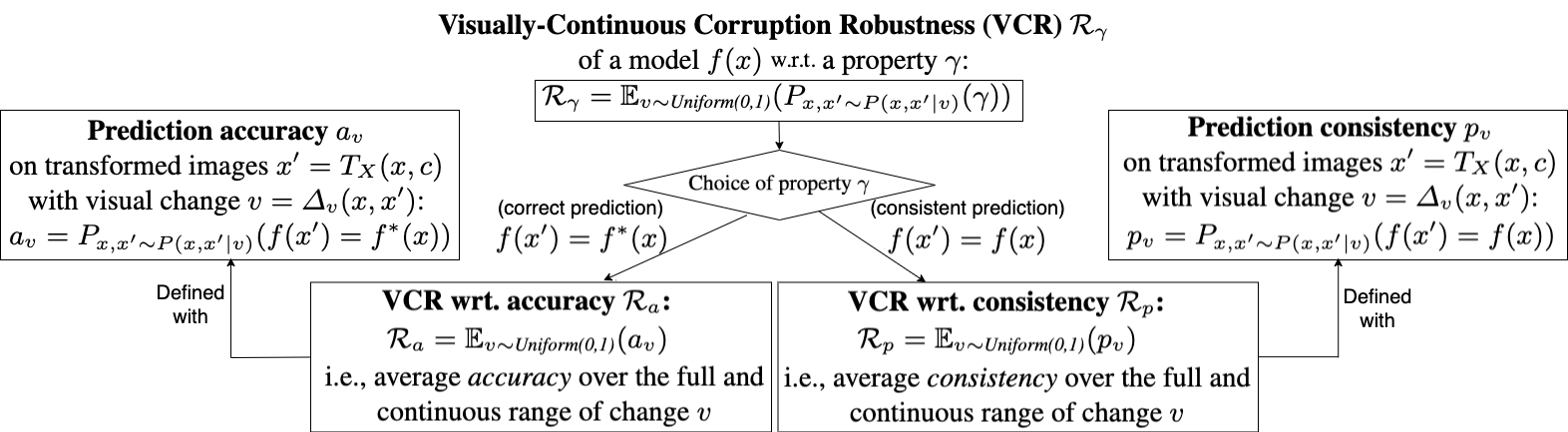
Figure 1: Summary of VCR definitions with respect to accuracy and consistency.

3.2 Testing VCR

VCR of a subject (a human or an NN) is measured by first generating a test set through sampling and then estimating it using the sampled data. The test set is generated by sampling images and applying corruption to obtain $P(x,x\textquoteright|v)$ for different $\Delta_{v}$ values $v$. We sample $x\sim P_{X}$ and $c\sim\textit{Uniform}(C)$, and obtain $x^{\prime}=T_{X}(x,c)$ and $v=\Delta_{v}(x,x^{\prime})$, resulting in samples $(x,x^{\prime},c,v)$. Then, we divide them into groups of $(x,x\textquoteright,c)$, each with the same $v$ value. Next, by dropping $c$, we obtain groups of $(x,x\textquoteright)$ with the same $v$, which are samples from $P(x,x\textquoteright|v)$. Note that this procedure requires only sufficient data in each group but not uniformity, i.e., $v\sim\textit{Uniform}(0,1)$ is not required. The varying size of each group, i.e., the non-uniformity of $v$ distribution, will not distort VCR estimates, but only impact the estimate uncertainty at a given $v$. Further, interpolation in the next step helps address any missing points.

With the test set, we estimate the performance w.r.t. the property $\gamma$ for each $v$. For each $v$ in the test data, we compute the rate of accurate predictions $f(x^{\prime})=f^{*}(x)$ to estimate accuracy, i.e., $a_{v}=P_{x,x^{\prime}\sim P(x,x^{\prime}|v)}(f(x^{\prime})=f^{*}(x))$ [resp. consistent predictions $f(x^{\prime})=f(x)$ to estimate consistency, i.e., $p_{v}=P_{x,x^{\prime}\sim P(x,x^{\prime}|v)}(f(x^{\prime})=f(x))$]. Then by plotting $(v,a_{v})$ and $(v,p_{v})$ and applying monotonic smoothing splines [25] to reduce randomness and outliers, we obtain smoothed spline curves $s_{a}$ and $s_{p}$, respectively. The curves $s_{\gamma}$ (namely, $s_{a}$ and $s_{p}$) describe how the performance w.r.t. the robustness property $\gamma$ (namely, $a$ and $p$) decreases as the visual corruption in images increases. Finally, we estimate $\mathcal{R}_{a}=\mathbb{E}_{v\sim\textit{Uniform(0,1)}}(a_{v})$ [resp. $\mathcal{R}_{p}=\mathbb{E}_{v\sim\textit{Uniform(0,1)}}(p_{v})$] as the area under the spline curve, i.e., $\hat{\mathcal{R}}_{a}=A_{a}=\int_{0}^{1}s_{a}(v)dv$ [resp. $\hat{\mathcal{R}}_{p}=A_{p}=\int_{0}^{1}s_{p}(v)dv$]. See Alg. 1 in the Appendix for the pseudo-code of VCR estimation.

3.3 Human-Aware Metrics for VCR

A commonly used metric for measuring corruption robustness is the Corruption Error (CE) [15]—the top-1 classification error rate on the corrupted images, normalized by the error rate of a baseline model. CE can be used to compare an NN with humans if the baseline model is set to be humans. However, CE is not able to determine whether an NN can exceed humans, and NN models could potentially have super-human accuracy for particular types of perturbations or in some $\Delta_{v}$ ranges. Therefore, inspired by CE, we propose two new human-aware metrics, Human-Relative Model Robustness Index (HMRI) that measures NN VCR relative to human VCR; and Model Robustness Superiority Index (MRSI) that measures how much an NN exceeds human VCR.

Auxiliary VCR metrics to compute HMRI and MRSI . HMRI and MRSI take as inputs the estimated spline curves for humans ($s^{h}_{\gamma}$) and for NN ($s^{m}_{\gamma}$). We denote areas under these curves as $A^{h}_{\gamma}$ and $A^{m}_{\gamma}$, respectively (see Fig. 2(a)). To compare NN model and human performance, VCR w.r.t. prediction consistency or accuracy is estimated using Alg. 1 using both model and human performance data, as illustrated by the yellow ($A^{h}_{\gamma}$) and blue ($A^{m}_{\gamma}$) areas Fig. 2(a), respectively. Both the blue and yellow areas also include the green area representing their overlap. Additionally, the VCR lead of humans over a model $A^{h>m}_{\gamma}$, the girded area in Fig. 2(a), and the VCR lead of a model over humans $A^{m>h}_{\gamma}$, the striped area in Fig. 2(a), are estimated. The definitions of these four auxiliary metrics are summarized in Tab. 2(b), and they are used to define HMRI and MRSI.

Definition 1 (Human-Relative Model Robustness Index (HMRI))

Given $s_{\gamma}^{h}$ and $s_{\gamma}^{m}$, let $A_{\gamma}^{h>m}=\int_{0}^{1}(s^{h}_{\gamma}(v)-s^{m}_{\gamma}(v))^{+}dv$ denote the average (accuracy or preservation) performance lead of humans over a model across the visual change range, where the performance lead is defined as the positive part of performance difference, i.e., $(s^{h}_{\gamma}(v)-s^{m}_{\gamma}(v))^{+}=max(0,s^{h}_{\gamma}(v)-s^{m}_{\gamma}(v))$. HMRI, which quantifies the extent to which a DNN can replicate human performance, is defined as $\frac{A^{h}_{\gamma}-A^{h>m}_{\gamma}}{A^{h}_{\gamma}}=1-\frac{A^{h>m}_{\gamma}}{A^{h}_{\gamma}}$.

The HMRI value ranges from $[0,1]$; a higher HMRI indicates a NN model closer to human VCR, and $\textit{HMRI}=1$ signifies that $s^{m}$ is the same as or completely above $s^{h}$ in the entire $\Delta_{v}$ domain, i.e., the NN is at least as robust as an average human (see Fig. 2(a)).

Definition 2 (Model Robustness Superiority Index (MRSI))

Given $s_{\gamma}^{h}$ and $s_{\gamma}^{m}$, let $A^{m>h}_{\gamma}=\int_{0}^{1}(s_{\gamma}^{m}(v)-s_{\gamma}^{h}(v))^{+}dv$ denote the average performance lead of a model over a human across the visual change range. MRSI, which quantifies the extent to which a DNN model can surpass human performance, is defined as $\frac{A^{m>h}_{\gamma}}{A^{m}_{\gamma}}$.

The MSRI value ranges from $[0,1)$, with the higher value indicating better performance than humans. $\textit{MSRI}=0$ means that the given NN model performs worse than or equal to humans in the entire $\Delta_{v}$ domain. A positive MSRI value indicates that the given NN model performs better than humans at least in some ranges of $\Delta_{v}$ (see Fig. 2(a)).

Comparing humans and NNs with HMRI and MRSI yields three possible scenarios: (1) humans’ performance fully exceeds NN’s, i.e., $0<\textit{HMRI}<1$ and $\textit{MRSI}=0$; (2) NN’s performance fully exceeds humans’, i.e., $\textit{HMRI}=1$ and $\textit{MRSI}>0$ ; and (3) humans’ performance is better than NN’s in some $\Delta_{v}$ intervals and worse in others, i.e., $\textit{HMRI}<1$ and $\textit{MRSI}>0$.

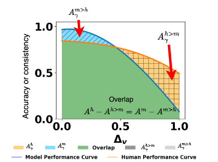
(a) Visualization of auxiliary metrics for model vs. human performance.

Auxiliary metric (cf. Fig. 2(a))
VCR of humans wrt. a property $\gamma$, estimated as an area under performance curve $A^{h}_{\gamma}$: $\hat{\mathcal{R}}_{\gamma}^{h}=A^{h}_{\gamma}=\int_{0}^{1}\ s^{h}_{\gamma}(v)dv$
VCR of a model $f(x)$ wrt. a property $\gamma$, estimated as an area under performance curve $A^{m}_{\gamma}$: $\hat{\mathcal{R}}_{\gamma}^{m}=A^{m}_{\gamma}=\int_{0}^{1}s^{m}_{\gamma}(v)dv$
VCR lead of humans over a model $f(x)$ wrt. a property $\gamma$, estimated as a difference area $A^{h>m}_{\gamma}$: $\hat{\mathcal{R}}_{\gamma}^{h>m}=A^{h>m}_{\gamma}$ $=\int_{0}^{1}\max(0,s^{h}_{\gamma}(v)-s^{m}_{\gamma}(v))dv$
VCR lead of a model $f(x)$ over humans wrt. a property $\gamma$, estimated as a difference area $A^{m>h}_{\gamma}$: $\hat{\mathcal{R}}_{\gamma}^{m>h}=A^{m>h}_{\gamma}$ $=\int_{0}^{1}\max(0,s^{m}_{\gamma}(v)-s^{h}_{\gamma}(v))dv$

(b) Summary of auxiliary metrics for defining HMRI and MRSI.

Figure 2: Auxiliary VCR metrics to compute HMRI and MSRI.

4 Experiments

In this section, we describe experiments that check the VCR of NN models against human performance.

NN models. Tab. 1 summarizes the models included in our study. We have selected a wide range of architectures (different CNN and transformer architectures) and training methods (supervised, adversarial, semi-weakly, and self-supervised), including dinov2_giant [34], which is on the top of the ImageNet-C leaderboard as of time of writing. In total, we studied 11 standard supervised models, 4 adversarial learning models, 2 SWSL models, 1 CLIP (clip-vit-base-patch32) model and 3 ViT models. For CLIP, we used the prompt “a picture of (ImageNet class)” while tokenizing the labels.

Model	Architecture	Training Method	Model	Architecture	Training Method
NoisyMix [5]	ResNet-50	Supervised	NoisyMix_new [5]	ResNet-50	Supervised
SIN [11]	ResNet-50	Supervised	SIN_IN [11]	ResNet-50	Supervised
SIN_IN_IN [11]	ResNet-50	Supervised	HMany [14]	ResNet-50	Supervised
HAugMix [17]	ResNet-50	Supervised	Standard_R50 [12]	ResNet-50	Supervised
AlexNet [26]	AlexNet	Supervised	Tian_DeiT-S [47]	DeiT Small	Supervised ViT
Tian_DeiT-B [47]	DeiT Base	Supervised ViT	Do_50_2_Linf [40]	WideResNet-50-2	Adversarial
Liu_Swin-L [29]	Swin-L	Adversarial	Liu_ConvNeXt-L [43]	ConvNeXt-L	Adversarial
Singh_ConvNeXt-L-ConvStem [43]	ConvNeXt-L + ConvStem	Adversarial	swsl_resnet18 [49]	ResNet-18	Semi-weakly sup.
swsl_resnext101_32x16d  [49]	ResNext-101	Semi-weakly sup.	CLIP [37]	Clip	Supervised CLIP
dinov2_giant [34]	ViT	Self-supervised ViT

Table 1: Summary of the models included in our study.

Image Corruptions. As shown in Fig. 3, we focus on studying VCR of NNs in relation to humans regarding 14 commonly used image corruptions from three different sources: Shot Noise, Impulse Noise, Gaussian Noise, Glass Blur, Gaussian Blur, Defocus Blur, Motion Blur, Brightness and Frost from ImageNet-C [15]; Blur, Median Blur, Hue Saturation Value and Color Jitter from Albumentations [1]; and Uniform Noise from [8].

noise
blur
others

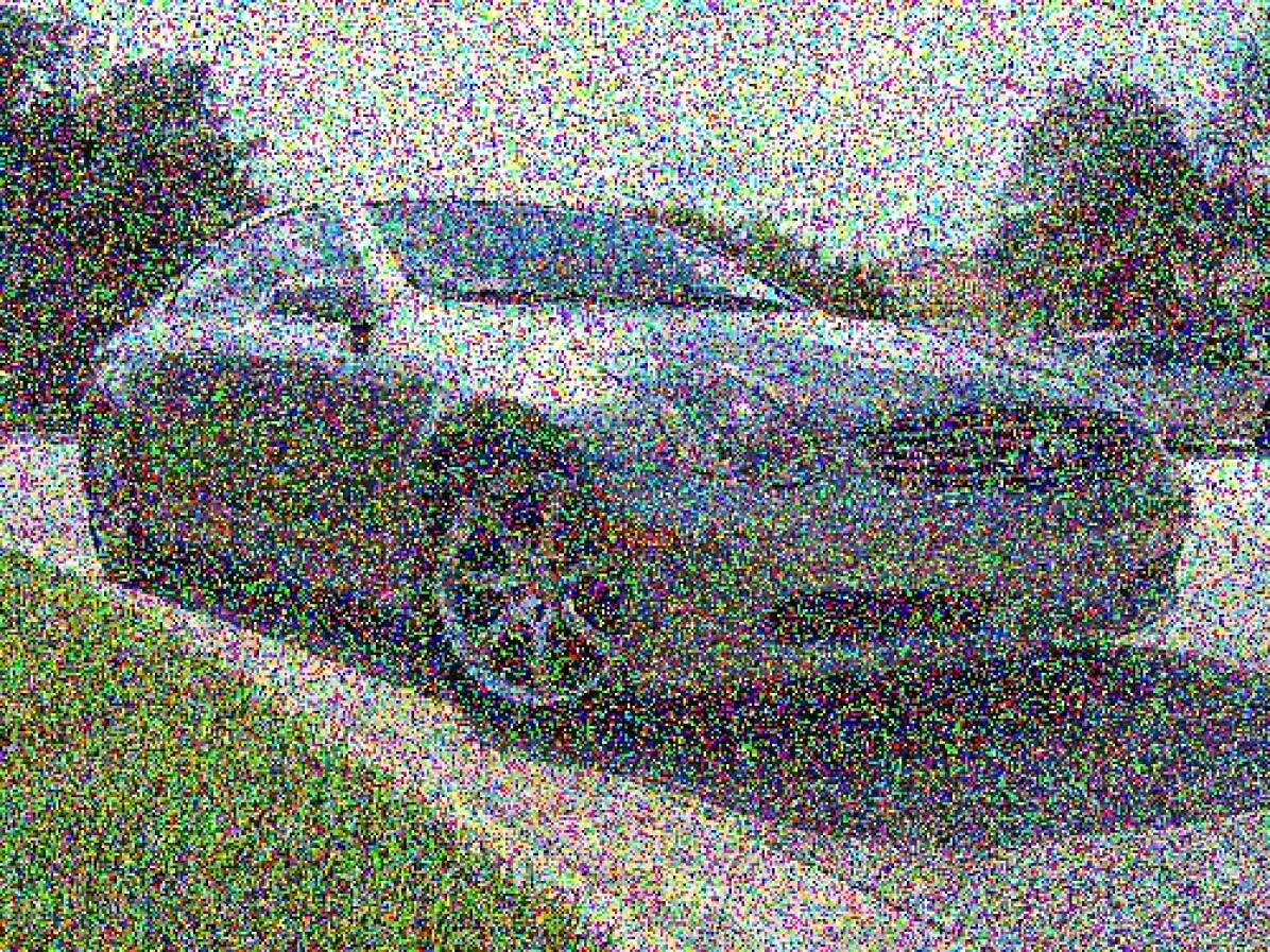
(a) Impulse Noise (ImageNet-C)

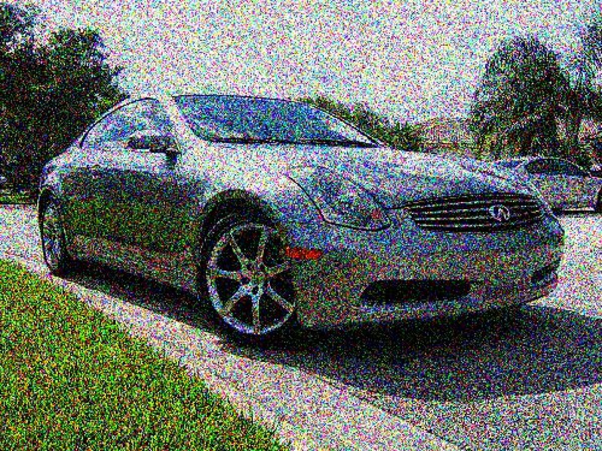
(b) Shot Noise (ImageNet-C)

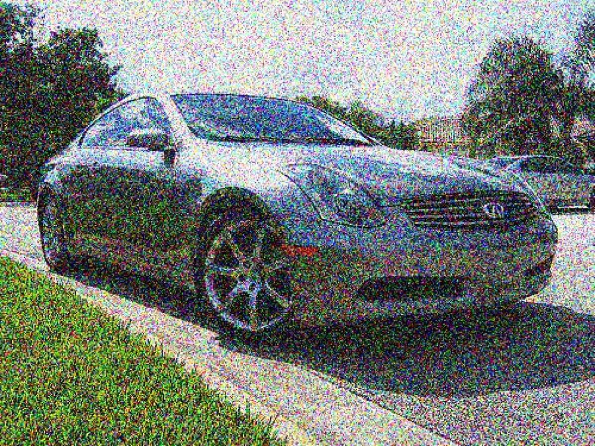
(c) Gaussian Noise (ImageNet-C)

(d) Uniform Noise ([8])

(e) Blur (Albumentation)

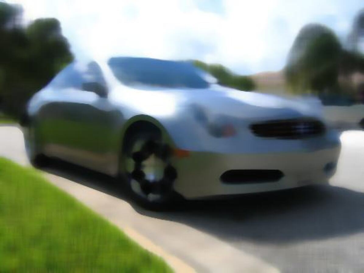
(f) Median Blur (Albumentation)

(g) Glass Blur (ImageNet-C)

(h) Gaussian Blur (ImageNet-C)

(i) Defocus Blur (ImageNet-C)

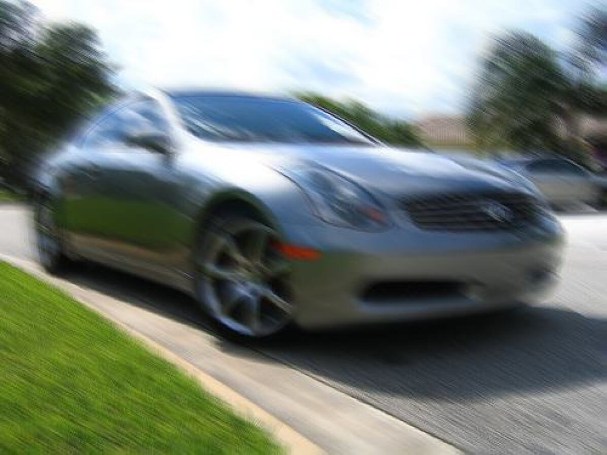
(j) Motion Blur (ImageNet-C)

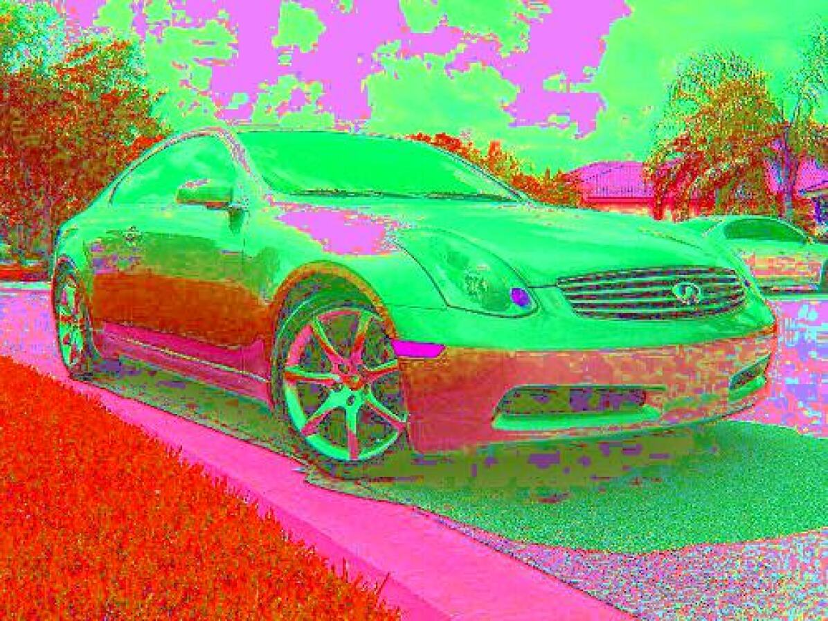
(k) Hue Saturation Value (Albumentation)

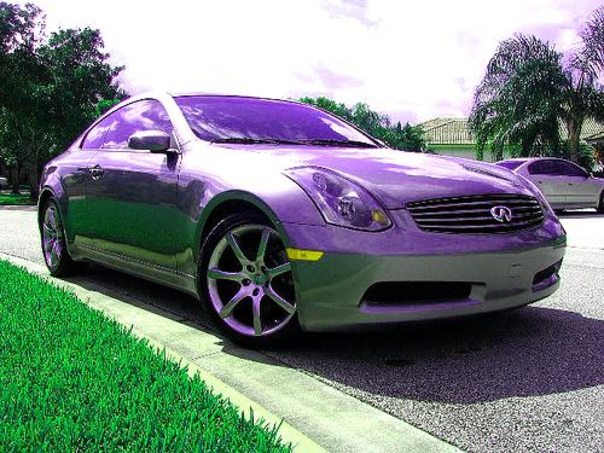
(l) Color Jitter (Albumentation)

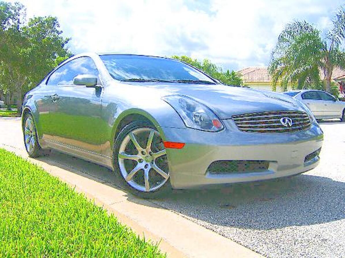
(m) Brightness (ImageNet-C)

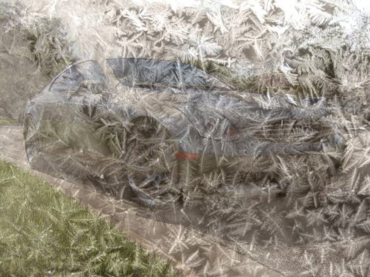
(n) Frost (ImageNet-C)

Figure 3: Image corruption functions.

Crowdsourcing. Given that VCR is focused on the average-case performance, we chose to use crowdsourcing for measuring human performance. This allowed us to involve a large number of participants for a more precise estimation of the average-case human performance. The experiment is designed following [20] and [8]. The experiment procedure is a forced-choice image categorization task: humans are presented with one image at a time, for 200 ms to limit the influence of recurrent processing, and asked to choose a correct category out of 16 entry-level class labels [8]. For NN models, the 1,000-class decision vector was mapped to the same 16 classes using the WordNet hierarchy [8]. The time to classify each image was set to ensure fairness in the comparison between humans and machines [6]. Between images, we showed a noise mask to minimize feedback influence in the brain [8]. We included qualification tests and sanity checks aimed to filter out cases of participants misunderstanding the task and spammers [35], and only considered results from those participants who passed both tests. As a result, we had $7{,}718$ participants and obtained approximately (1) $70{,}000$ human predictions on images with different levels of visual corruptions; and (2) $50{,}000$ human predictions on original images as these can be repeated in experiments for different corruptions. The same original image, corrupted or not, was never shown again to the same participant.

4.1 Experiment 1: Testing Robustness against Visual Corruption

ImageNet-C is the SoTA benchmark for corruption robustness. Rather than considering the continuous range of corruption like VCR, ImageNet-C includes all ImageNet validation images corrupted using 5 pre-selected parameter values for each type of corruption [15]. This section compares robustness measured with ImageNet-C vs. VCR on all 9 ImageNet-C corruption functions in our study. Due to the page limit, we include full results in the appendix.

Visual Corruption in Test Sets. For each corruption, our tests generated for checking VCR contain $50,000$ images, mirroring the size of the ImageNet [39] validation set, while ImageNet-C includes $5\times 50,000$ images. Due to the difference in how test sets are generated, we observe two major differences in the distributions of degrees of visual corruption: they have different coverage and peak at different values (e.g., Fig. 4).

To quantitatively assess the actual coverage of $\Delta_{v}$ in the test sets, Tab. 2 gives the coverage as a percentage of the full $\Delta_{v}$ range of $[0,1]$. To compute it, the distribution is divided into 40 bins with the same width. A bin is considered covered if it contains 20 or more images. The coverage is then determined by dividing the number of covered bins by the total number of bins (40). We observed that ImageNet-C exhibits a low coverage of $\Delta_{v}$ values. Specifically, as shown in Fig. 4 and Tab. 2, the distribution of ImageNet-C in Gaussian blur has coverage of only 56.4% focusing mainly on the center of the entire domain of $\Delta_{v}$ and missing coverage for low and high $\Delta_{v}$ values, which can lead to biased evaluation. As we show in the appendix, the same can be observed for most ImageNet-C corruption functions. On the other hand, our test sets provide coverage for almost the entire domain, with a coverage percentage of 97.4%. This pattern holds true for other corruption functions as well—our test sets have consistently higher coverage than ImageNet-C. As for VCR, Shot Noise and Impulse Noise have relatively low coverage, because the level of noise these functions add is exponential to their parameters. As a result, uniform sampling of the parameter range $C$ fails to cover small $\Delta_{v}$ values. When using uniform sampling over $C$, reaching the full coverage of $\Delta_{v}$ would require a large amount of data. Note, however, Alg. 1 still computes VCR over the full $\Delta_{v}$ range of $[0..1]$, and the lack of samples for low values of $\Delta_{v}$ has a limited impact on the VCR estimate. This is because we fit a monotonic spline that is anchored with a known initial performance for $\Delta_{v}=0$, as discussed in Appendix. 0.D.

Remark: The reported accuracy of ImageNet-C can be directly impacted both by a lack of coverage and by non-uniformity, as it is computed as the average accuracy of all corrupted images. In contrast, the shape of the $\Delta_{v}$ distribution in the test images does not impact VCR once sufficient coverage is achieved to estimate the spline curves $s_{\gamma}$.

(a) ImageNet-C.

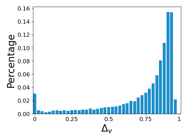
(b) VCR Test Set.

Figure 4: Histograms showing $\Delta_{v}$ distribution between ImageNet-C and our VCR test sets for Gaussian Blur.

Corruption	Coverage
	ImageNet-C	VCR Test Set
Brightness	0.590	1.000
Gaussian Blur	0.564	0.974
Defocus Blur	0.538	0.923
Shot Noise	0.462	0.590
Frost	0.436	1.000
Gaussian Noise	0.436	0.872
Impulse Noise	0.385	0.641
Motion Blur	0.333	0.974
Glass Blur	0.333	0.949

Table 2: $\Delta_{v}$ Coverage Comparison with ImageNet-C.

Robustness Evaluation Results. Next, we compare robustness evaluation results obtained with ImageNet-C and VCR test sets. Consider results for Gaussian Noise in Fig. 5. NoisyMix and NoisyMix_new have almost the same robust accuracy on ImageNet-C, but NoisyMix_new has higher $\hat{\mathcal{R}}_{a}$; similarly, SIN has higher ImageNet-C robust accuracy but lower $\hat{\mathcal{R}}_{a}$ than SIN_IN_IN. This is due to the almost complete lack of coverage for $\Delta_{v}<0.5$ for Gaussian Noise in ImageNet-C (see Tab. 2), which can lead to biased evaluation results (i.e., biased towards $\Delta_{v}\geq 0.5$). Checking VCR allows us to detect such biases.

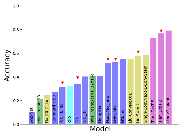
(a) ImageNet-C Gaussian Noise Accuracy.

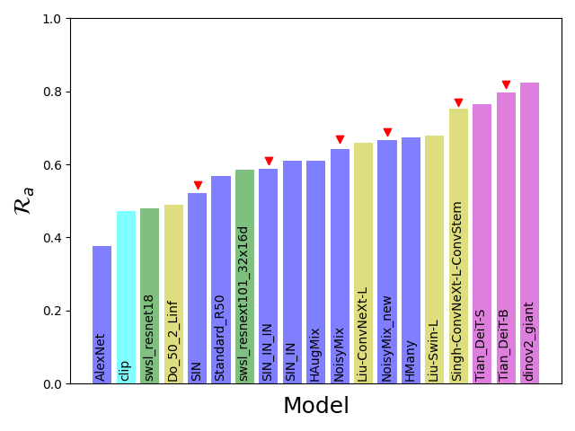
(b) Gaussian Noise $\hat{\mathcal{R}}_{a}$.

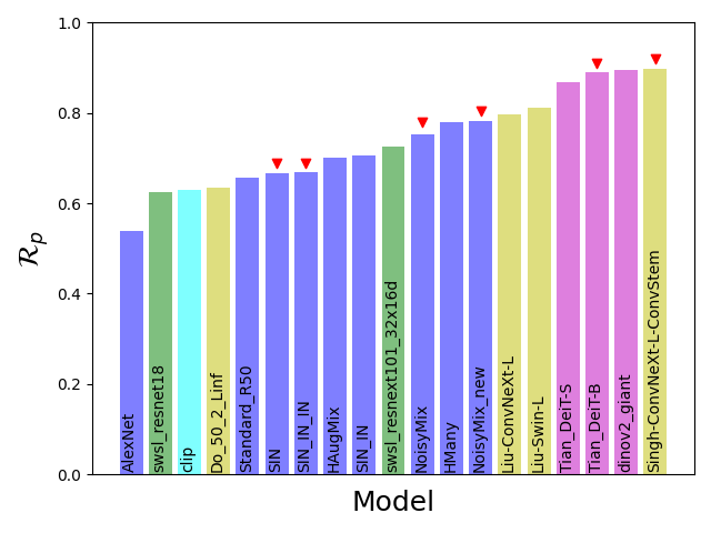
(c) Gaussian Noise $\hat{\mathcal{R}}_{p}$.

Figure 5: Comparison between ImageNet-C and VCR with Gaussian Noise. Models discussed in the text are marked by a red triangle.

In addition to accuracy, VCR can also check whether the NN can preserve its predictions after corruption, i.e., the prediction consistency property $p$, giving additional information about NN robustness. From Figs. 5(b), 5(c), we can see that the model Tian_Deit_B has a higher $\hat{\mathcal{R}}_{a}$ than Singh-ConvNeXt-L-ConvStem but a lower $\hat{\mathcal{R}}_{p}$. This suggests that even though Tian_Deit_B has better accuracy for corrupted images, it labels the same image with different labels before and after the corruption. Since ground truth can be hard to obtain during deployment, having low prediction consistency indicates issues with model stability and could raise concerns about when to trust the model prediction. Results for the remaining corruptions are in Appendix. 0.E.

Summary: It is essential to test robustness before deploying NNs into an environment with a wide and continuous range of visual corruptions. Our results confirmed that testing robustness in this range using a fixed and pre-selected number of parameter values can lead to undetected robustness issues, which can be avoided by checking VCR. Additionally, accuracy cannot accurately represent model stability when facing corruptions, which can be addressed by testing $\mathcal{R}_{p}$.

4.2 Experiment 2: VCR of DNNs Compared with Humans

In this experiment, we use our new human-aware metrics, HMRI and MRSI, and the data from the human experiment data to compare VCR of the studied models against human performance.

For Gaussian Noise, Fig. 7 presents our measured HMRI and MRSI values for $\mathcal{R}_{a}$ and $\mathcal{R}_{p}$. For both metrics, a higher value indicates better robustness. As shown in Fig. 6(a), no NN has reached $1.0$ for $\textit{HMRI}_{a}$, and in Fig. 6(d), only 3 out of 21 NNs dinov2_giant, Tian_DeiT-B and Singh-ConvNeXt-L-ConvStem reached $1.0$ for $\textit{HMRI}_{p}$, indicating that there are still unclosed gaps between human and NN robustness, with humans giving more accurate and more consistent predictions facing corruptions than most SoTA NNs. These thee top-performing models have also the highest HMRI values for both $\mathcal{R}_{a}$ and $\mathcal{R}_{p}$, making these models closest to human robustness. In Fig. 6(b), we can see that these three models have $\textit{MRSI}_{a}$ values above $0.0$, indicating that they surpass human accuracy in certain ranges of visual corruption. This can be visualized by checking the estimated curves $s_{a}$ as shown in Fig. 6(c). The top-three models exceed human accuracy (the red curve) when $\Delta_{v}>0.85$. For prediction consistency, Fig. 6(e) shows that all NNs have the $\textit{MRSI}_{p}$ value above $0.0$ and this is because, as shown in Fig. 6(f), all NN curves are above the human curve when the $\Delta_{v}$ value is small. Specifically, the top-three models completely exceed humans in the entire $\Delta_{v}$ range.

Similarly, for Uniform Noise, as shown in Fig. 6(g) and Fig. 6(j), no models reached $1.0$ for $\textit{HMRI}_{a}$ and the top-three models, reached $1.0$ for $\textit{HMRI}_{p}$. Together with Fig. 6(h) and Fig. 6(k), we can see that for both $\mathcal{R}_{a}$ and $\mathcal{R}_{p}$, Tian_DeiT-B has higher HMRI values but Tian_DeiT-S has higher MRSI values. This suggests that while Tian_DeiT-B is closer to human performance, Tian_DeiT-S exceeds human performance more. This result may be counter-intuitive but can be explained with the curves $s_{a}$ and $s_{p}$ representing how the performance w.r.t. the robustness properties $a$ and $p$ decreases as $\Delta_{v}$ increases, as shown in Fig. 6(i) and Fig. 6(l). From both $s_{a}$ and $s_{p}$, we observed that for $\Delta_{v}$ values less than $0.8$, the performance of Tian_DeiT-B is higher than Tian_DeiT-S and closer to human, hence the higher HMRI value; and after $\Delta_{v}=0.8$ when human performance starts decreasing, the Tian_DeiT-B performance drops rapidly to much below that of Tian_DeiT-S, hence the lower MRSI value.

This suggests that both HMRI and MRSI are useful for comparing NN robustness, and our curves $s_{a}$ and $s_{p}$ can provide further information on NN robustness with different degrees of visual corruption.

Overall, in both Fig. 7 and Fig. 7, we observed that the three ViT models (shown in purple) have the best performance for both $\mathcal{R}_{a}$ and $\mathcal{R}_{p}$, making them the models closest to human robustness. The same can also be observed for the rest of the corruption functions; see the appendix for more details. This indicates that vision transformer is the most promising architecture for reaching human-level robustness, even outperforming models trained with additional training data. The data in the appendix also indicates the biggest remaining robustness gap for blur corruptions. Furthermore, our generated test sets can be used during model retraining for improved robustness compared to humans, resulting in with higher HMRI and MRSI values.

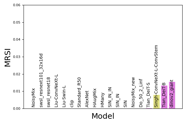
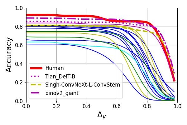
(a) HMRI for $\mathcal{R}_{a}$	(b) MRSI for $\mathcal{R}_{a}$	(c) Estimated curves $s_{a}$
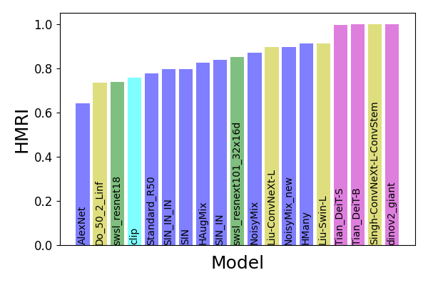
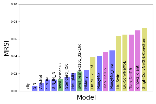
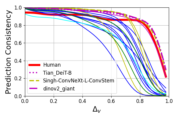
(d) HMRI for $\mathcal{R}_{p}$	(e) MRSI for $\mathcal{R}_{p}$	(f) Estimated curves $s_{p}$

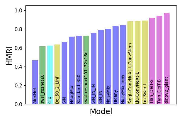
Figure 6: VCR evaluation results for Gaussian Noise. Results include, for each NN, the estimated curves $s_{a}$ and $s_{p}$ (representing how the performance w.r.t. the robustness properties $a$ and $p$ decreases as $\Delta_{v}$ increases); and the corresponding HMRI and MRSI values. Results are colored based on their category: Human, Vision Transformer, Supervised Learning, SWSL, Adversarial Training, CLIP.

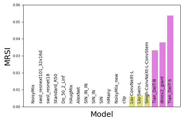
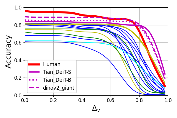
(g) HMRI for $\mathcal{R}_{a}$	(h) MRSI for $\mathcal{R}_{a}$	(i) Estimated curves $s_{a}$
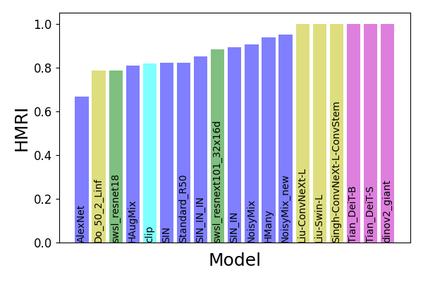
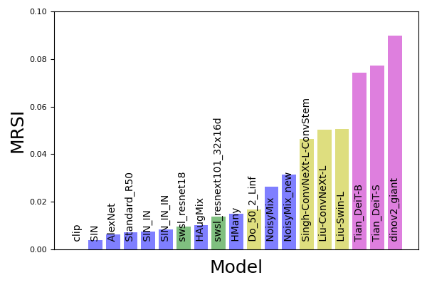
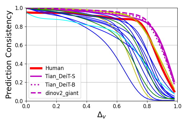
(j) HMRI for $\mathcal{R}_{p}$	(k) MRSI for $\mathcal{R}_{p}$	(l) Estimated curves $s_{p}$

Figure 7: VCR evaluation results for Uniform Noise.

Summary: As our results suggest, when considering the full range of visually-continuous corruption, no NNs can match human accuracy, especially for blur corruptions, and only the best-performing ones can match human prediction consistency. For some specific degrees of corruption, few NNs can exceed humans by mostly tiny margins. This highlights a more substantial gap between human and NN robustness than previously identified by [10]. By evaluating VCR using our human-centric metrics, we gain deeper insights into the robustness gap, which can aid in the development of models closer to human robustness.

4.3 Experiment 3: Training with Data Augmentation

Because VCR considers a different distribution of corruptions in the images (i.e., continuous) than existing benchmarks (i.e., selected parameter values), model performance is expected to improve once the model is fine-tuned on the new distribution. We show a small retraining example to demonstrate the usefulness of our benchmark in improving VCR. The retraining process was carried out by fine-tuning all parameters of the image classification model. The training dataset was generated from a subset sampled from the ImageNet [39] training set with a size of around 12,000. For optimization, we leveraged the most basic stochastic gradient descent with learning rate=0.001 and momentum=0.9. We utilized Cross-Entropy Loss as the loss function, given its effectiveness in classification tasks. The number of epochs depends on the model. Five epochs are usually enough to show some progress. The state-of-the-art NNs are already optimized for the corruption functions included in ImageNet-C; however, as shown in Tab. 2, for certain corruption functions, such as Motion Blur, Frost and Glass Blur, ImageNet-C images do not cover a wide range of visual changes, leaving room for robustness improvement. In Tab. 3, we demonstrate results for NNs SIN [11] and Standard_R50 [3] for these corruption functions, the rest can be found in the codebase${}^{\ref{git}}$.

Summary: Our results show that simply retraining with tests generated with VCR can improve all metrics comparing NN model performance relative to humans, even for models already optimized for the same corruption functions included in ImageNet-C. This is because VCR considers a completely different distribution of corruption that the models were not previously exposed to. This shows that the gap between human and NN robustness is larger than benchmarks with discrete corruptions such as ImageNet-C can detect. Our proposed VCR can not only detect this gap, it also provides a step towards closing this gap!

	Results for Standard_R50 [3]												Results for SIN [11]
	Before Retraining						After Retraining						Before Retraining						After Retraining
	Accuracy			Prediction similarity			Accuracy			Prediction similarity			Accuracy			Prediction similarity			Accuracy			Prediction similarity
corruption function	$\hat{\mathcal{R}}_{a}$	HMRI	MRSI	$\hat{\mathcal{R}}_{p}$	HMRI	MRSI	$\hat{\mathcal{R}}_{a}$	HMRI	MRSI	$\hat{\mathcal{R}}_{p}$	HMRI	MRSI	$\hat{\mathcal{R}}_{a}$	HMRI	MRSI	$\hat{\mathcal{R}}_{p}$	HMRI	MRSI	$\hat{\mathcal{R}}_{a}$	HMRI	MRSI	$\hat{\mathcal{R}}_{p}$	HMRI	MRSI
Median Blur	0.532	0.635	0.000	0.573	0.673	0.000	0.694	0.828	0.003	0.728	0.854	0.001	0.522	0.624	0.00	0.605	0.710	0.00	0.650	0.774	0.004	0.729	0.852	0.004
Frost	0.429	0.521	0.011	0.473	0.572	0.012	0.575	0.690	0.025	0.678	0.804	0.031	0.423	0.512	0.015	0.513	0.618	0.016	0.517	0.625	0.016	0.647	0.768	0.031
Glass Blur	0.468	0.569	0.003	0.502	0.603	0.003	0.647	0.770	0.024	0.744	0.866	0.034	0.334	0.407	0.000	0.397	0.478	0.000	0.572	0.687	0.016	0.684	0.809	0.018
Note: all numbers are rounded.

Table 3: VCR comparison before and after retraining. Red indicates improvement.

4.4 Experiment 4: VCR for Visually Similar Corruption Functions

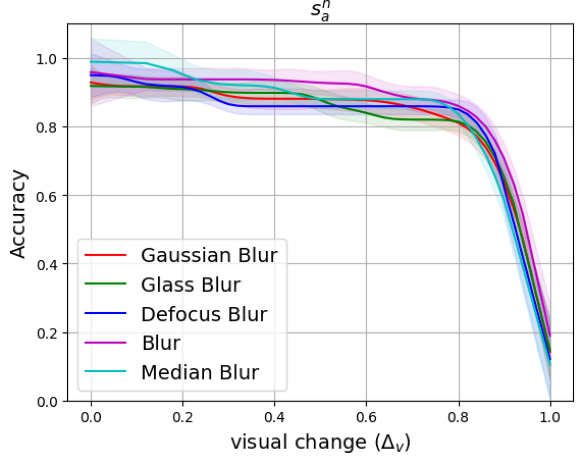
(a) Blur class $s_{a}^{h}$

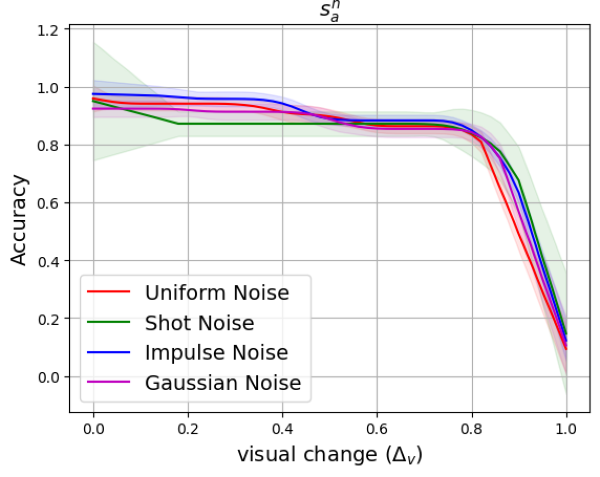
(b) Noise class $s_{a}^{h}$

(c) Dissimilar $s_{a}^{h}$

Figure 8: Comparing human performance spline curves $s^{h}_{a}$ for similar and dissimilar corruption functions. For each curve, the coloured region around the curve is the $83\%$ confidence interval used for comparison of similarity. See $s^{h}_{p}$ in Appendix. 0.E.

One noteworthy observation we made from our experiments with humans is the existence of visually similar corruption functions. This can contribute towards reducing experiment costs and a better understanding of differences between humans and NNs.

Different corruptions change different aspects of the images, e.g., image colour, contrast, and the amount of additive visual noise, and thus affect human perception differently [8]. Also, multiple different corruption functions can be implemented for the same visual effect, such as Gaussian noise and Impulse noise for noise addition. Although the difference between Gaussian noise and Impulse noise can be picked up by complex NN models, an average human would struggle to distinguish between the two. Therefore, for a specific visual effect, there should exist a class of corruption functions implementing the effect that an average human is unable to tell them apart. We call corruption functions in the same class visually similar. We postulate that since visually similar functions, by definition, affect human perception similarly, they would affect human robustness similarly as well. Therefore, human data for one function can be reused for other similar functions in the same class possibly reducing experiment costs.

Since VCR is estimated with the spline curves $s_{a}^{h}$ and $s_{p}^{h}$, if the difference among the curves of a set of functions is statistically insignificant, human data (i.e., the spline curves) can be reused among the functions in this set. In Fig. 8, we plot the smoothed spline curves $s_{a}^{h}$ and $s_{p}^{h}$ obtained for all 14 corruption functions included in our experiments. We can observe that, for all corruption functions shown, human performance decreases slowly for small values of visual degrade ($\Delta_{v}$), but once $\Delta_{v}$ reaches a turning point, human performance starts decreasing more rapidly. Then, we observe that spline curves obtained for certain blur and noise transformations have similar shapes, while those for dissimilar transformations start decreasing at different turning points with different slopes. More specifically, the differences between two spline curves are statistically insignificant if their $83\%$ confidence intervals overlap [25].

Summary: By checking statistical significance with $83\%$ confidence interval for each corruption function, we empirically observed two classes of visually similar corruptions in our experiments with humans: (1) the noise class: Shot Noise, Impulse Noise, Gaussian Noise, and Uniform Noise; and (2) the blur class: Blur, Median Blur, Gaussian Blur, Glass blur, Defocus Blur. The remaining corruptions are dissimilar (see Fig. 8).

NN Robustness for Visually Similar Corruption Functions. Because of the central difference between humans and NNs, e.g., computational powers, it is intuitive that NNs might react completely differently to corruptions visually similar to humans, and using VCR, we can empirically analyze such difference. For example, during deployment, noise with unknown distributions (ranging from Uniform, Gaussian, Poisson etc.), can be encountered. While noise distribution does not affect humans as we showed in Fig. 8, NNs which are particularly susceptible to a certain distribution might raise safety concerns. For example, two visually similar transformations Gaussian Noise and Uniform Noise add an additional noise to the images with the Gaussian and the Uniform distribution, respectively. However, our results in Fig. 7 and Fig. 7 suggest that the distribution difference is picked up by NNs. We can observe that most models have higher HMRI and MRSI values for Uniform Noise than Gaussian Noise. For small amounts of corruption ($\Delta_{v}<0.8$), the difference between the estimated $s_{a}$ and $s_{p}$ curves for both corruptions is not statistically significant, i.e., NN models perform similarly when facing small amounts of Uniform and Gaussian Noise. For $\Delta_{v}$ values between $[0.8..1.0]$, most visual information required for humans to recognize objects is corrupted by the noise, human performance decreases quickly, but the most robust models, e.g., dinov2_giant and Tian_DeiT-S, are able to pick up more information than humans and make reasonable recognition. When the added noise is from a uniform distribution, NN models perform better than when it is from a Gaussian distribution. Therefore, studying VCR also allows us to empirically analyze how changing the noise distribution, which would not affect humans, affects NN performance for different degrees of corruption. In the case of unknown or shifting distributions, such analysis would require human data for all distributions which is impractical and expensive. Identifying classes of visually similar corruption functions and reusing human data would significantly reduce the experiment costs.

Identifying Visually Similar Transformations. We provide a naive method for identifying classes of visually similar corruptions. To identify whether two corruptions are similar enough to reuse human data, the goal is to determine whether the difference between them is distinguishable to a human. This can be done through a set of relatively inexpensive experiments. Without knowing the specific corruptions introduced to the images, participants are shown corrupted images and asked if the presented images are corrupted with the same corruption function. Presented images can be corrupted with the same or different corruption functions. Then, by repeating the experiments with different sampled images, the accuracy of distinguishing the corruptions can be calculated. We hypothesize that if the corruption functions are indistinguishable, human accuracy should be close to random. Then, since each experiment is either successfully distinguished or not, we use a binomial test to check whether the accuracy is statistically significant to not be random. Visually similar transformations included in this paper can be detected with this naive method. Our experiments showed that for each pair of transformations, results with statistical significance can be reached in less than a minute. Compared to the full set of experiments with $2{,}000$ images and five different participants for each experiment, identifying similar transformations significantly decreased the experiment time, from approximately $5.55$ hours to $5$ minutes.

Limitation: Note that the results of this method can be highly dependent on the opinion of the participants; thus, it is more optimal to select participants with a normal eyesight and a basic knowledge of image corruptions. We acknowledge that this naive method cannot give the most accurate identification of visually similar transformations. For example, it is reasonable to assume that two transformations can have very different visual effects but still affect human robustness in the same way, and this case would not be detected with this method. Nevertheless, we hope that our findings will promote future investigations of how NNs and humans react differently to corruptions.

5 Conclusion

In this paper, we revisit corruption robustness to consider it in relation to the wide and continuous range of corruptions to human perceptive quality, defining visually-continuous corruption robustness (VCR); along with two novel human-aware metrics for NN evaluation. Our results showed that the robustness gap between human and NNs is bigger than previously detected, especially for blur corruptions. We found that using the full and continuous range of visual change is necessary when estimating robustness, as insufficient coverage can lead to biased results. We also discovered classes of image corruptions that affect human perception similarly and identifying them can help reduce the cost of measuring human robustness and assessing disparities between human perception and computational models. In our study, we only considered the comparison of object recognition between humans and NNs; however, human and machine vision can be compared in many different ways, e.g., against neural data [50, 27], contrasting Gestalt effects [24], object similarity judgments [13], or mid-level properties [45]. Still, we hope our results will inspire future robustness studies. We also provide our benchmark datasets with human performance data and our code as open source.

Appendix 0.A Implementation and Data

Data and implementation can be found at https://github.com/HuakunShen/reliabilitycli.

Appendix 0.B Overview of VCR-Bench

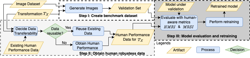
Figure 9: Our proposed method VCR-Bench for benchmarking ML robustness with humans.

Our method for benchmarking VCR (VCR-Bench) is outlined in Fig. 9. Step I generates a validation set that covers the full continuous range of visual changes. This is achieved by uniformly sampling from the entire domain of corruption function parameters. Step II obtains human robustness performance data needed to compute our two newly-proposed human-aware evaluation metrics: Human-Relative Model Robustness Index (HMRI) and Model Robustness Superiority Index (MRSI), which quantify the extent to which a NN can replicate or surpasses human performance, respectively. Since measuring human performance for every single image corruption function is expensive and impractical, we propose a method to reduce the cost by generalizing existing human performance data obtained for one corruption function to a class of corruption functions with similar visual effects. For example, images transformed with Gaussian Blur and Glass Blur have very similar visual effects on humans, unlike Motion Blur and Brightness. Thus, Gaussian Blur and Glass Blur, but not with Motion Blur and Brightness, thus they belong to the same class of similar corruption functions, and human performance data for one can be transferred to the other. Step III of VCR-Bench evaluates the model using the validation dataset and our human-aware metrics. Then it retrains the model to improve its robustness.

Appendix 0.C VCR and Its Estimation

Background: Image Quality Assessment (IQA). IQA metrics serve as quantitative measures of human objective image quality [48]. By comparing the original image and the transformed image, IQA metrics automatically estimate the perceived image quality by evaluating the perceptual “distance” between the two images [41]. This “distance” differs from simple pixel distance and varies depending on the specific IQA metric used.

One such metric is VIF (Visual Information Fidelity) [41], which evaluates the fidelity of information by analyzing the statistical properties of natural scenes within the images. VIF returns a value between 0 and 1 if the changes degrade perceived image quality, with 1 indicating the perfect quality compared to the original image; and it returns a value $>1$ if the changes enhances image quality [41]. More precisely, VIF defines the visual quality of a distorted image as a ratio of the amount of information a human can extract from the distorted image versus the original reference image. The method models statistically (i) images in the wavelet domain with coefficients drawn from a Gaussian scale mixture, (ii) distortions as attenuation and additive Gaussian noise in the wavelet domain, and (iii) the human visual system (HVS) as additive white Gaussian noise in each sub-band of the wavelet decomposition. The amount of information that a human can extract from the distorted image is measured as the mutual information between the distorted image and the output of the HVS model for that image. Similarly, the amount of information that a human can extract from the reference image is measured as the mutual information between the reference image and the output of the HVS model for that image. Empirical studies have shown that VIF aligns closely with human opinions when compared to other IQA metrics [42].

We choose VIF, since it is well-established, computationally efficient, applicable to our transformations, and still performing competitively compared to newer metrics. More recent research has explored the use of feature spaces computed by deep NNs as a basis to define IQA metrics (e.g., LPIPS [56] and DISTS [4]). Even though these metrics may be applicable to a wider class of transformations than VIF, including those that affect both structure and textures, their scope may depend on the training datasets in potentially unpredictable ways. On the other hand, the scope of VIF is well-defined based on the metric’s mathematical definition. In particular, VIF is suitable for evaluating corruption functions that can be locally described as a combination of signal attenuation and additive Gaussian noise in the sub-bands of the wavelet domain [41]. The transformations in our experiments are local corruptions that are well within this scope. Moreover, VIF performs still competitively when compared to even the newer DNN-based metrics across multiple datasets (e.g., see Table 1 in [4]). However, future work should explore VCR using other IQA metrics.

Visual Change ($\Delta_{v}$). The metric $(\Delta_{v})$ defined using the IQA metric VIF, as shown in Def. 3, is proposed by Hu et al. [20] to quantitatively measure the amount of visual changes in the images perceived by human observers.

Definition 3

Let an image $x$, an applicable corruption function $T_{X}$ with a parameter domain $C$ and a parameter $c\in C$, s.t. $x^{\prime}=T_{X}(x,c)$ be given. Visual change $\Delta_{v}(x,x^{\prime})$ is a function defined as follows:

$$\begin{cases}0&$If VIF$(x,x^{\prime})>1\\ 1-$VIF$(x,x^{\prime})&$Otherwise $\end{cases}$$

$\Delta_{v}$ returns a value between 0 and 1, with 0 indicating no degradation to visual quality and 1 indicating all visual information in the original image has been changed. The first case of $\Delta_{v}$ corresponds to changes that enhance the visual quality (when VIF$(x,x^{\prime})>1$), indicating changes do not impact human recognition of the images negatively, hence $\Delta_{v}=0$. The other case deals with visible changes that degrade visual quality. Since VIF returns 1 for perfect quality compared to the original image, the degradation is one minus the image quality score.

Example: In Fig. 10, the visual change of the original image Fig. 10(a) is $0$, since no changes are applied; and Fig. 10(b) has minimal frost added, which caused minimal change in visual quality so $\Delta_{v}=0.005$; and Fig. 10(c) and Fig. 10(d) have more frost and thus higher $\Delta_{v}$ values $0.71$ and $0.96$, respectively.

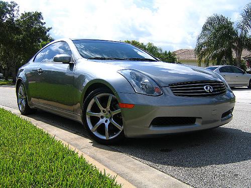
(a) original image, $\Delta_{v}=0$

(b) $\Delta_{v}=0.005$

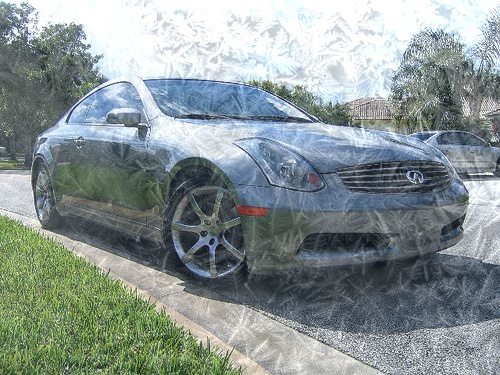
(c) $\Delta_{v}=0.71$

(d) $\Delta_{v}=0.96$

Figure 10: Examples of images from Imagenet [39] with different levels of added frost.

Input: $\begin{cases}\text{model }f(x)\\ \text{transformation }T_{X},\text{with parameter domain }C\\ \text{input dataset }\{x_{k}\}\text{ for consistency [or }\{(x_{k},y_{k})\}\text{ for accuracy]}\\ \text{generated test set size }N\\ \text{visual change resolution }M\\ \text{minimum number of points per bin }L\end{cases}$

Output: estimated VCR $\hat{\mathcal{R}}_{p}$ [or $\hat{\mathcal{R}}_{a}$]

Initialize histograms $\textit{count}_{j}$ and $\textit{correct}_{j}$ with empty counts, for all $j\in[0..M-1]$

Initialize performance data array $P_{j}$ with $-1$, denoting missing data points for $j$, for all $j\in[0..M-1]$

for $i\leftarrow 0\mathbf{~{}to~{}}N-1$ do

       draw random $x$ from $\{x_{k}\}$ [or $(x,y)$ from $\{(x_{k},y_{k})\}$]

       $c\sim\textit{Uniform}(C)$

       $x^{\prime}\leftarrow T_{X}(x,c)$

       $v\leftarrow\Delta_{v}(x,x^{\prime})$

       $j\leftarrow\lfloor v(M-1)\rfloor$

       $\textit{count}_{j}\leftarrow\textit{count}_{j}+1$

       if $f(x^{\prime})=f(x)$ [or $f(x^{\prime})=y$] then

             $\textit{correct}_{j}\leftarrow\textit{correct}_{j}+1$

      

for $j\leftarrow 0\mathbf{~{}to~{}}M-1$ do

       if $\textit{count}_{j}\geq L$ then

             $P_{j}\leftarrow\frac{\textit{correct}_{j}}{\textit{count}_{j}}$

      

$s\leftarrow\textit{FitMonotonicSpline}(P)$

$\hat{\mathcal{R}}\leftarrow\int_{0}^{1}s(v)dv$

return $\hat{\mathcal{R}}$

[2.5pt]

Algorithm 1 VCR Estimation

VCR Estimation Algorithm. Algorithm 1 gives the pseudo-code of the VCR estimation procedure described under “Testing VCR” in the main body of the paper. The algorithm takes a model $f(x)$; a transformation $T_{X}$ with its parameter domain $C$; an input dataset; the size $N$ of the dataset of transformed images to be generated; the visual change resolution $M$, over which the model performance will be estimated; and the minimum size $L$ of a bin to be used to estimate the performance for that bin. The input dataset consist of images $x_{k}\sim P_{X}$ for estimating VCR wrt. consistency, or images and their labels for estimating VCR wrt. accuracy. We use $M=40$ in our experiments, which is a standard choice for calculating average precision in object detection; for example, it is used in the current version of the KITTI benchmark [7].

Our algorithm first initializes two histogram arrays to keep the counts of the tested data points and their consistent or accurate predictions, respectively, and an array to keep the performance data, with each of the three arrays having size $M$. In each iteration, the first for-loop samples an image $x$ and transformation parameter $c$, and produces a transformed image $x^{\prime}$. It then computes the visual change value $v$ and records the result of testing $f(x^{\prime})$ in the histograms. The second for-loop computes the performance data as a relative frequency of correct predictions. A monotonic smoothing spline is fit into the performance data, and the VCR is computed as the area under the spline.

Note that this algorithm samples $c$ uniformly, which will lead to a varying number of performance samples per point in the performance data array $P$. As already discussed, the number of performance samples impacts the performance estimate uncertainty at this point, and in an extreme case some of the $\Delta_{v}$ bins in $P_{i}$ may be even empty (i.e., have value -1). These missing points are mitigated by fitting the spline over the entire $\Delta_{v}$ range, while anchoring it with known values for the first and last bins. In particular, the accuracy spline $s_{a}$ always starts at the left with the accuracy for clean images, and the consistency spline $s_{p}$ starts with 1 for models (assuming deterministic NNs).

A possible approach to obtain a sample set with a more uniform coverage of $\Delta_{v}$ would be to (1) fit a strictly monotonic spline into $(c,\Delta_{v})$ values obtained from $c\sim\textit{Uniform}(C)$ as in Alg. 1, (2) take a set of samples $\Delta_{v}\sim\textit{Uniform}(0,1)$, (3) map the latter to a new sample from $C$ using the inverted spline, and repeat these steps now using the new sample from $C$. These steps would need to be run iteratively until a sufficient coverage is obtained. Such an algorithm would be computationally expensive, however.

Appendix 0.D Comparison of $\Delta_{v}$ Distribution

In Fig. 11 below we compare the $\Delta_{v}$ distribution of validation images from ImageNet-C and those generated by our benchmark. We include all 9 corruption functions shared between ImageNet-C and our benchmark. Note that all of our images are generated by sampling uniformly in the parameter domain, while ImageNet-C images are generated with 5 pre-selected parameter values. We can observe two major differences in the distributions. First we can see that because of difference in the parameter values used, the $\Delta_{v}$ distributions between ImageNet-C and our benchmark peak at different values. For example, for Brightness in Fig. 11(a) and Fig. 11(b), most ImageNet-C images have $\Delta_{v}$ values between $0.4$ to $0.8$, while most VCR-Bench images are between $0.6$ and $0.9$; a similar observation holds for Defocus Blur and Gaussian Blur. Second, we notice that ImageNet-C images cannot cover all $\Delta_{v}$ values. Specifically, Fig. 11(c) for Defocus Blur shows that ImageNet-C validation set does not contain images with $\Delta_{v}$ greater than $0.8$ and less than $0.2$. The same can be observed for all corruption functions shown in Fig. 11. These two differences indicate that, when considering the full range of visual changes that a corruption function can incur, using ImageNet-C can lead to biased results.

Brightness		Defocus Blur		Gaussian Noise
Glass Blur		Impulse Noise		Shot Noise
Frost		Gaussian Blur		Motion Blur

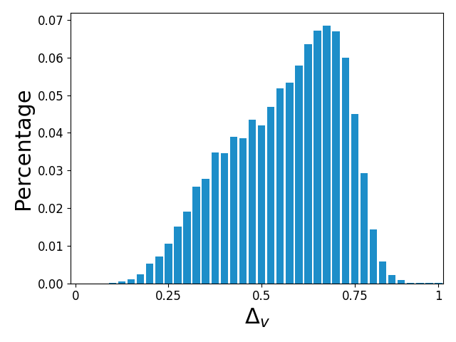
(a) ImageNet-C

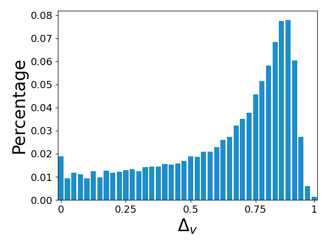
(b) VCR-Bench

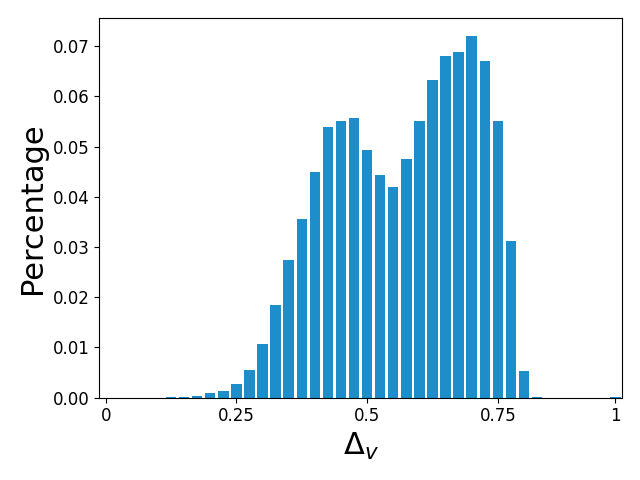
(c) ImageNet-C

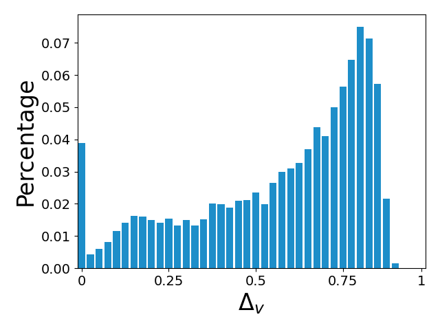
(d) VCR-Bench

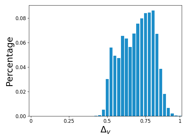
(e) ImageNet-C

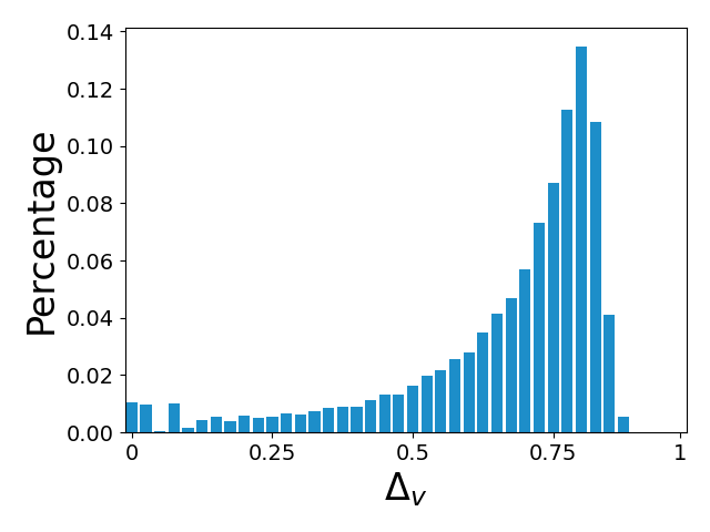
(f) VCR-Bench

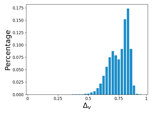
(g) ImageNet-C

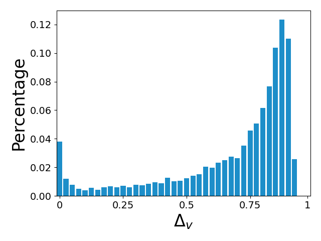
(h) VCR-Bench

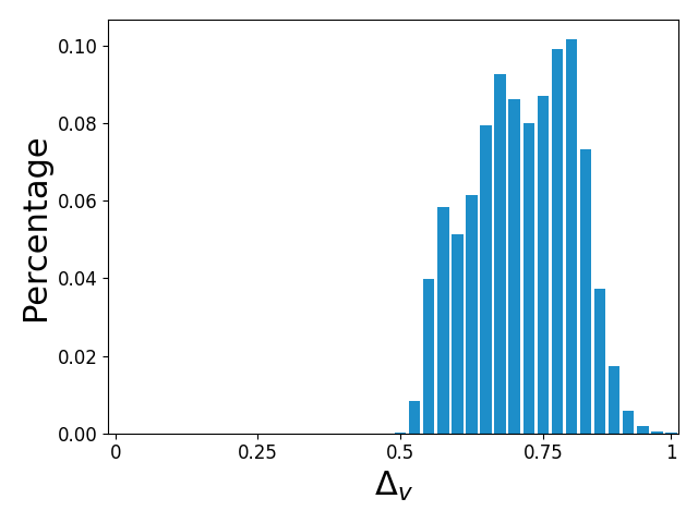
(i) ImageNet-C

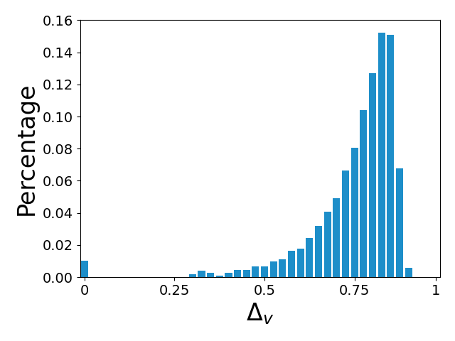
(j) VCR-Bench

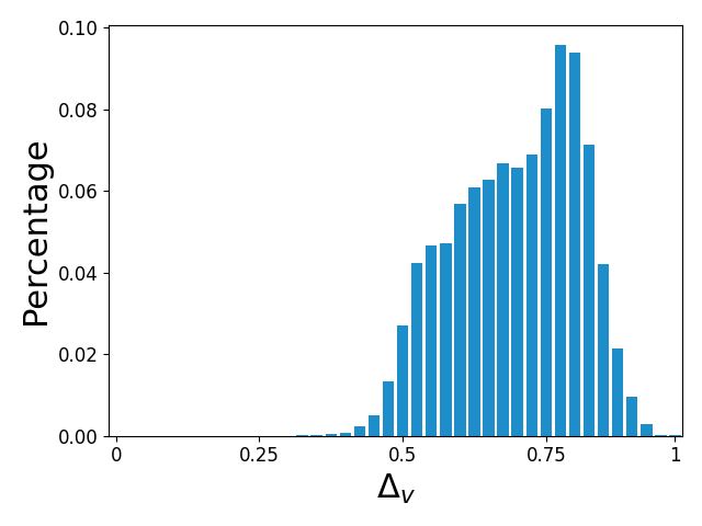
(k) ImageNet-C

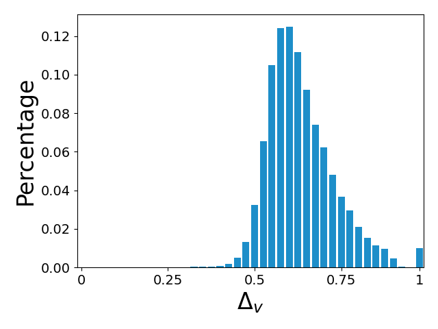
(l) VCR-Bench

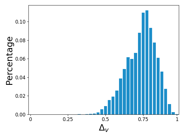
(m) ImageNet-C

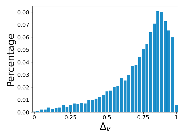
(n) VCR-Bench

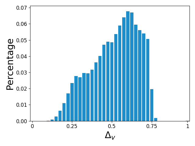
(o) ImageNet-C

(p) VCR-Bench

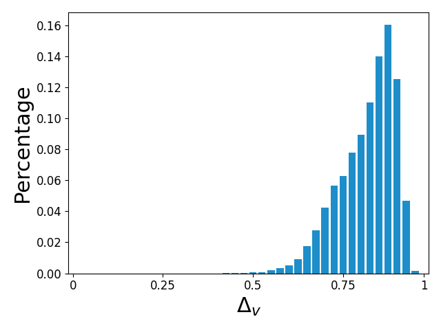
(q) ImageNet-C

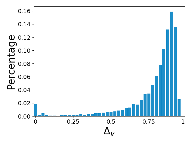
(r) VCR-Bench

Figure 11: Comparison of $\Delta_{v}$ distribution between ImageNet-C and VCR-Bench. The figures are histograms, where x-axis is $\Delta_{v}$, y-axis is percentage of images.

Appendix 0.E Extra Evaluation Results

0.E.1 Prediction Similarity of Visually Similar Corruption Functions

In the paper, to check that human robustness data is transferable between two similar corruption functions, we checked whether the $83\%$ confidence interval of the spine curves $s^{h}_{a}$ and $s^{h}_{p}$ for similar corruption functions overlap. The results for $s^{h}_{a}$ in Fig. 8. We also include results for $s^{h}_{p}$ in Fig. 12. We can observe that, similar to $s^{h}_{a}$, $s^{h}_{p}$ for similar corruption functions are similar, thus human data is transferable.

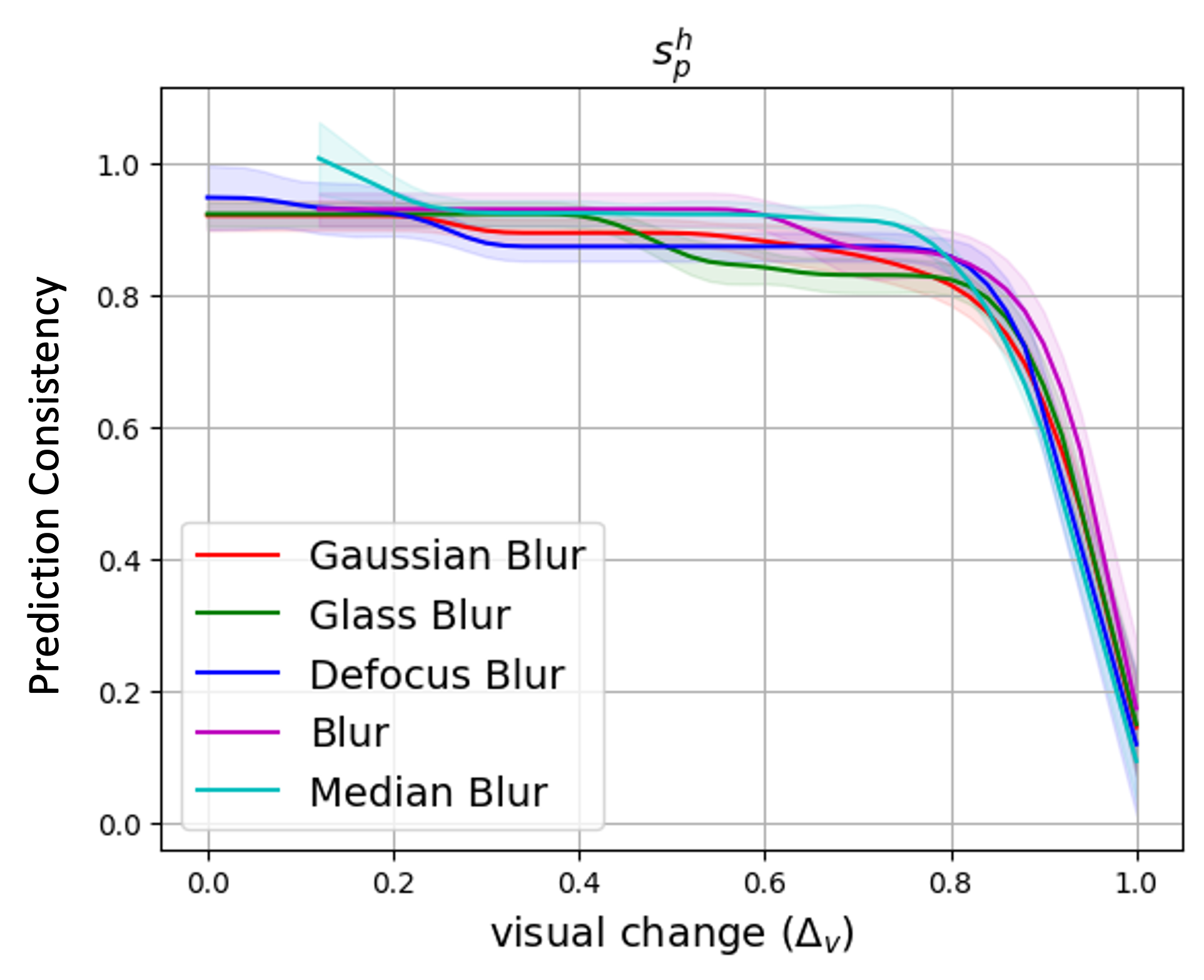
(a) Blur corruption functions

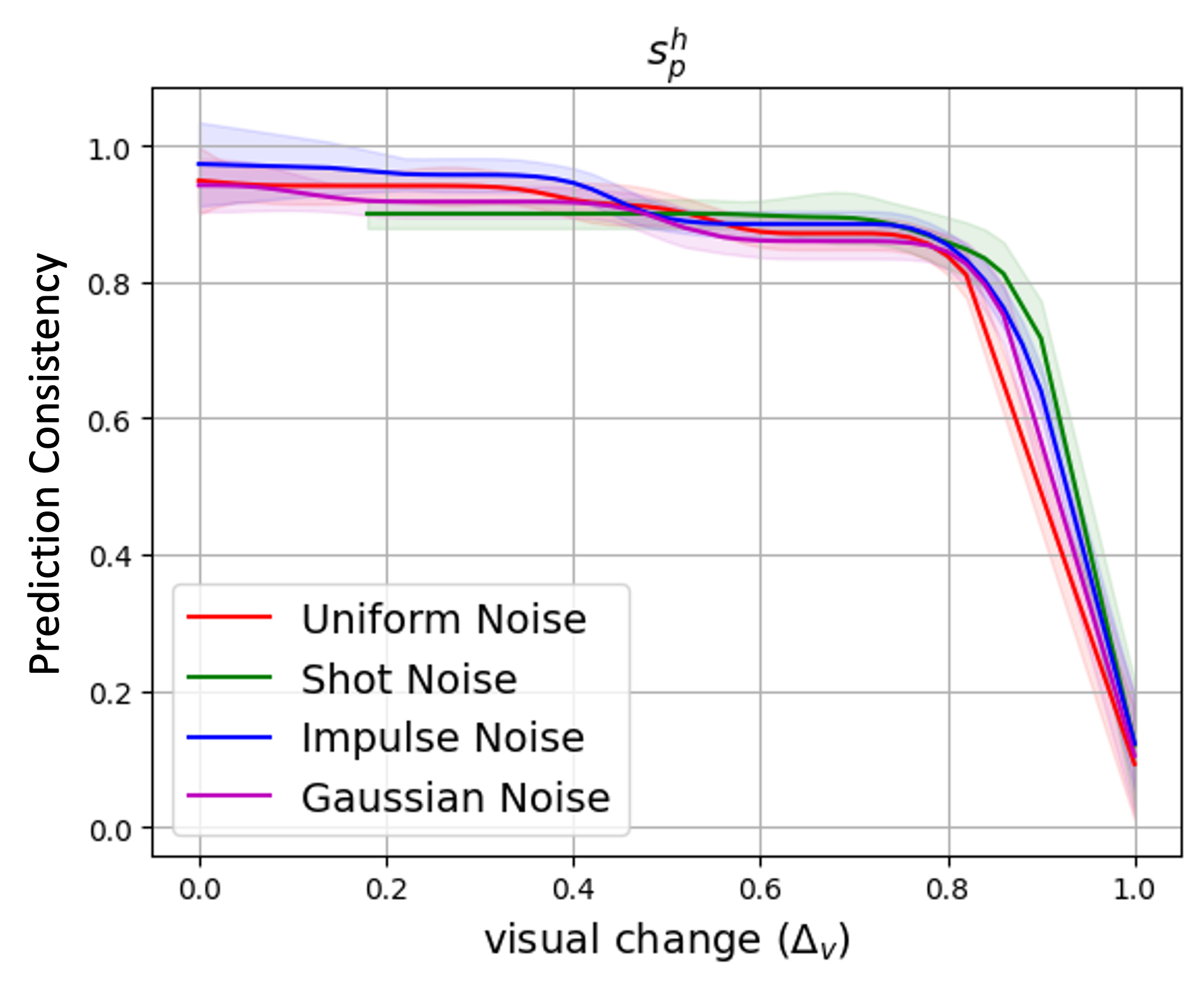
(b) Noise corruption functions

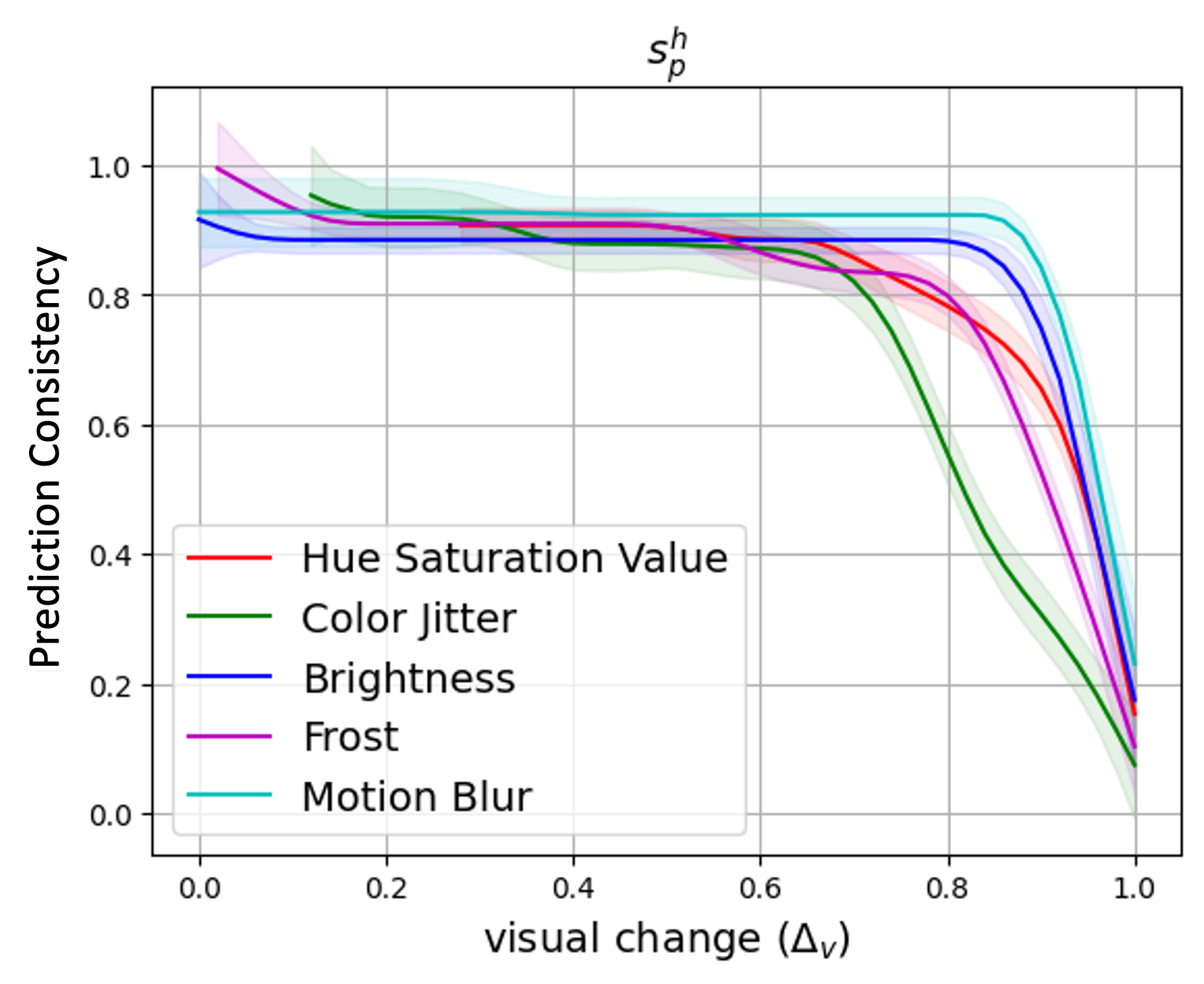
(c) Dissimilar corruption functions

Figure 12: Comparing human performance spline curves $s^{h}_{p}$ for similar and dissimilar corruption functions. For each curve, the coloured region around the curve is the $83\%$ confidence interval used for comparison of similarity [25].

0.E.2 CO2 Emission

CO2 Emission is calculated as CO2 emissions (kg) = (Power consumption in kilowatts) x (Daily usage time in hours) x (Emissions factor in kgCO2/kWh)

Our carbon intensity is around 25 g/kWh. During benchmark dataset generation, there is no GPU usage, and the CPU usage is 200 W. Each corruption function takes around 1.5 hour to generate a dataset with 50,000 images. During evaluation, the CPU power usage is around 160 W; and GPU power usage ranges between 50-170 W depending on the model. Each evaluation takes 30-60 minutes, depending on the corruption function type. Let’s assume the power usage of other components is 50 W in total. If we assume the total power usage is $((200+50)\times 1.5+(170+160+50))/1{,}000=0.755\,$kWh for each experiment, the CO2 emission is $0.755\times 25=18.875$ g for each experiment (corruption function type).

0.E.3 VCR Evaluation

In the main body of the paper, we have compared VCR robustness results with ImageNet-C on Gaussian Noise, and we presented the assessing VCR in relation to human performance with our human-aware metrics HMRI and MRSI for Gaussian Noise and Shot Noise. Below, we first include the comparison between VCR and ImageNet-C for all ImageNet-C 9 corruption functions we studied. Then, include detailed evaluation results with our human-aware metrics for all 12 other corruption functions we studied.

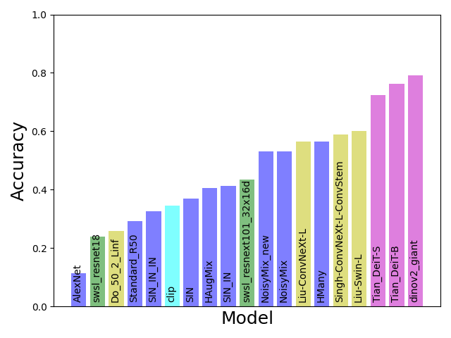
(a) ImageNet-C Gaussian Noise Accuracy

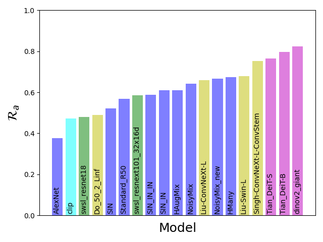
(b) Gaussian Noise $\hat{\mathcal{R}}_{a}$

(c) Gaussian Noise $\hat{\mathcal{R}}_{p}$

Figure 13: Comparison between ImageNet-C and VCR with Gaussian Noise.

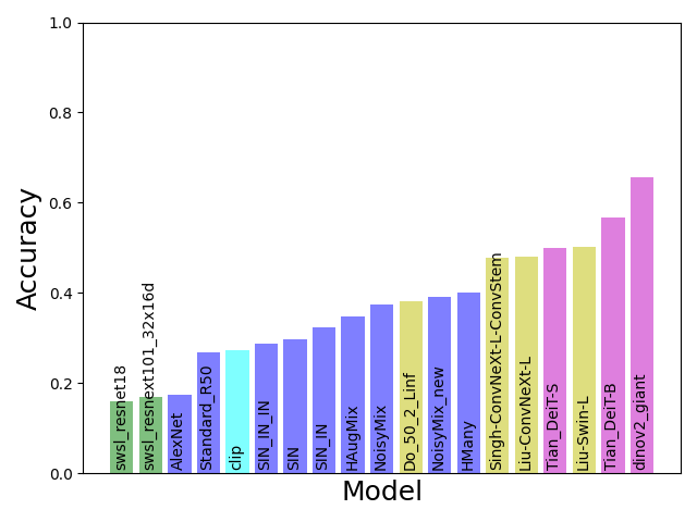
(a) ImageNet-C Glass Blur Accuracy

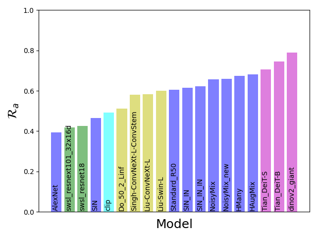
(b) Glass Blur $\hat{\mathcal{R}}_{a}$

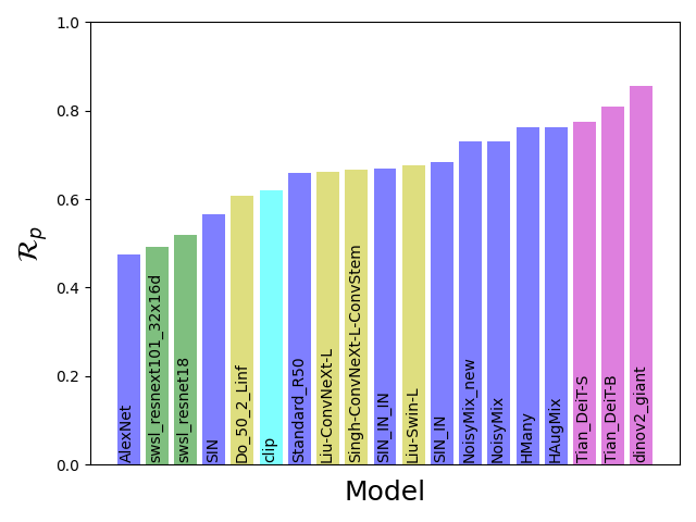
(c) Glass Blur $\hat{\mathcal{R}}_{p}$

Figure 14: Comparison between ImageNet-C and VCR with Glass Blur.

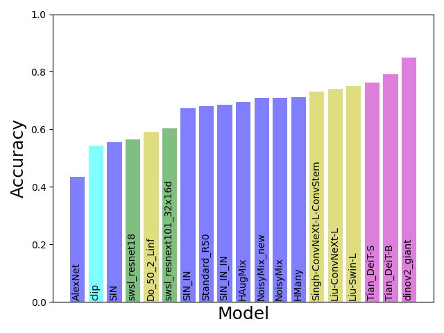
(a) ImageNet-C Brightness Accuracy

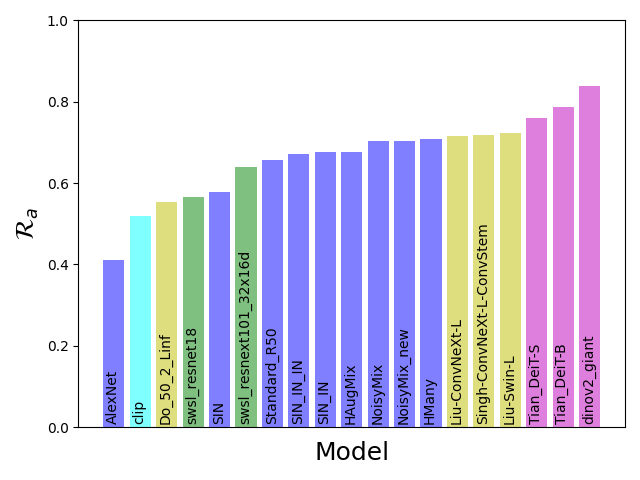
(b) Brightness $\hat{\mathcal{R}}_{a}$

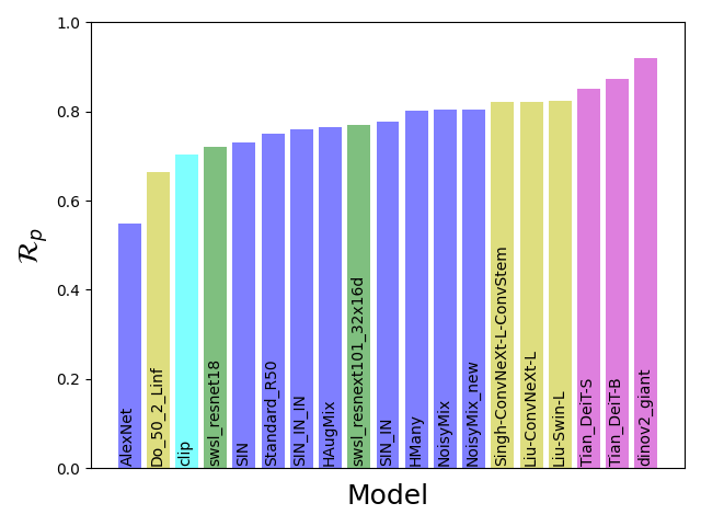
(c) Brightness $\hat{\mathcal{R}}_{p}$

Figure 15: Comparison between ImageNet-C and VCR with Brightness.

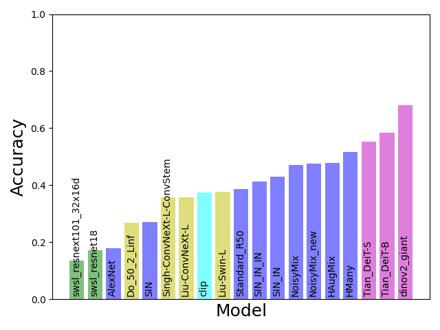
(a) ImageNet-C Defocus Blur Accuracy

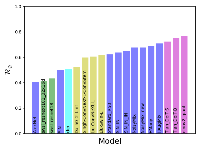
(b) Defocus Blur $\hat{\mathcal{R}}_{a}$

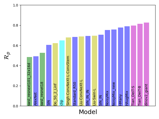
(c) Defocus Blur $\hat{\mathcal{R}}_{p}$

Figure 16: Comparison between ImageNet-C and VCR with Defocus Blur.

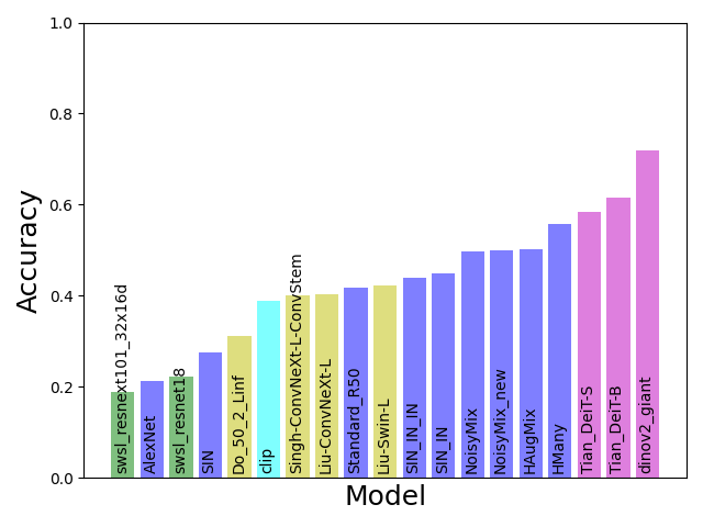
(a) ImageNet-C Gaussian Blur Accuracy

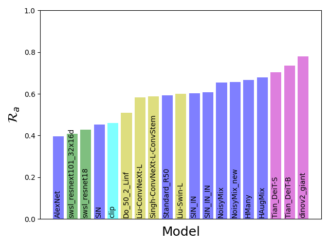
(b) Gaussian Blur $\hat{\mathcal{R}}_{a}$

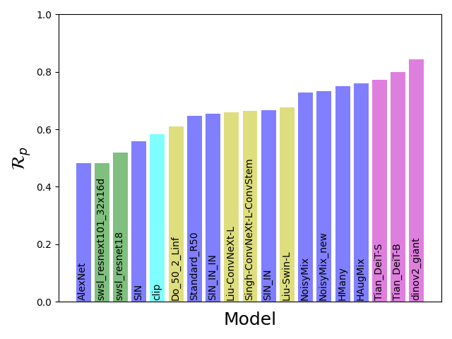
(c) Gaussian Blur $\hat{\mathcal{R}}_{p}$

Figure 17: Comparison between ImageNet-C and VCR with Gaussian Blur.

(a) ImageNet-C Shot Noise Accuracy

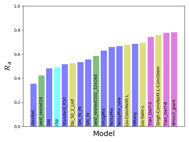
(b) Shot Noise $\hat{\mathcal{R}}_{a}$

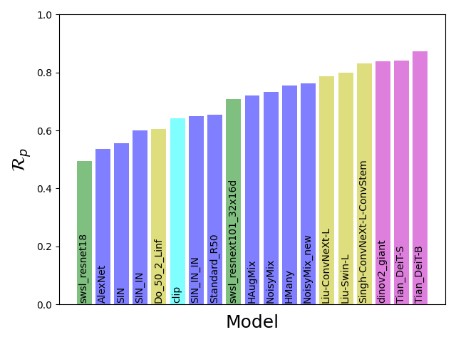
(c) Shot Noise $\hat{\mathcal{R}}_{p}$

Figure 18: Comparison between ImageNet-C and VCR with Shot Noise.

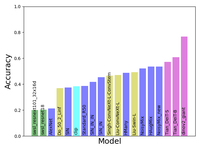
(a) ImageNet-C Motion Blur Accuracy

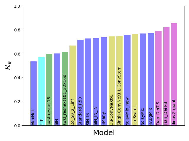
(b) Motion Blur $\hat{\mathcal{R}}_{a}$

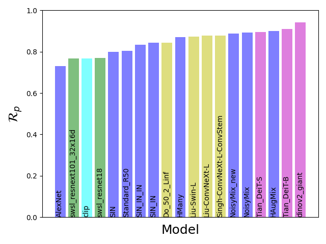
(c) Motion Blur $\hat{\mathcal{R}}_{p}$

Figure 19: Comparison between ImageNet-C and VCR with Motion Blur.

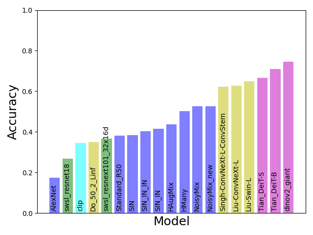
(a) ImageNet-C Frost Accuracy

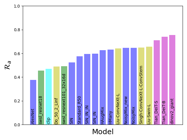
(b) Frost $\hat{\mathcal{R}}_{a}$

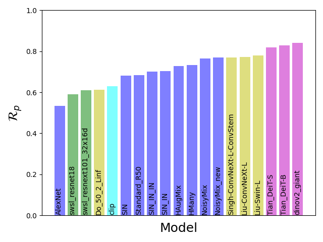
(c) Frost $\hat{\mathcal{R}}_{p}$

Figure 20: Comparison between ImageNet-C and VCR with Frost.

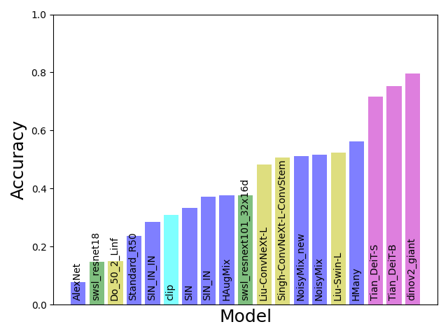
(a) ImageNet-C Impulse Noise Accuracy

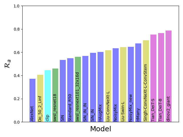
(b) Impulse Noise $\hat{\mathcal{R}}_{a}$

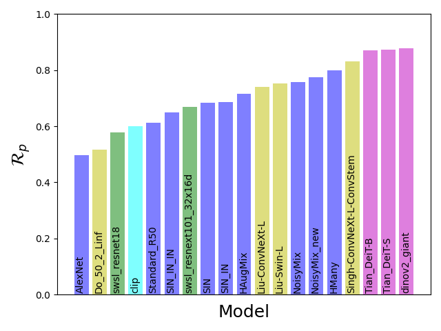
(c) Impulse Noise $\hat{\mathcal{R}}_{p}$

Figure 21: Comparison between ImageNet-C and VCR with Impulse Noise.

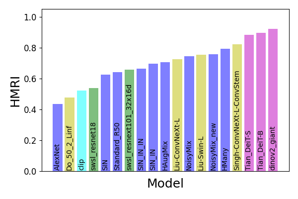
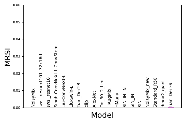
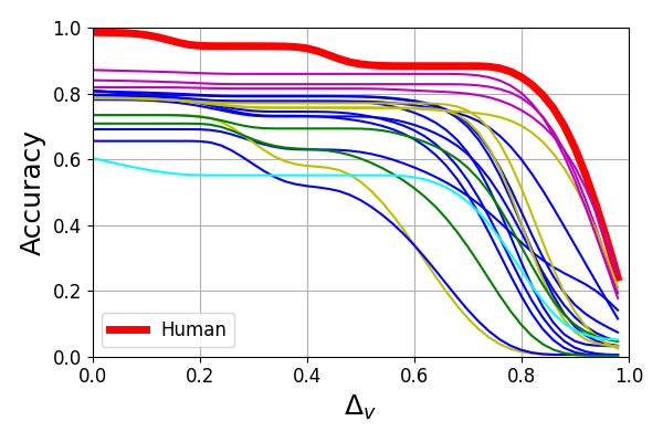
(a) HMRI for $\mathcal{R}_{a}$	(b) MRSI for $\mathcal{R}_{a}$	(c) Estimated curves $s_{a}$
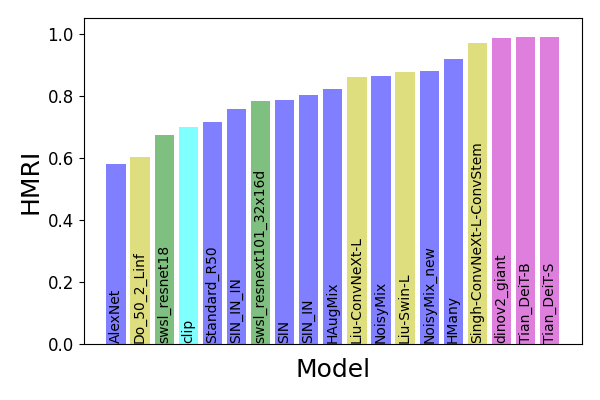
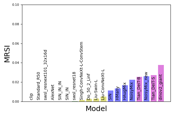
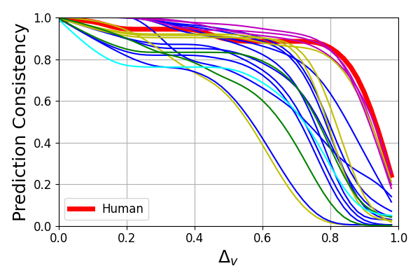
(d) HMRI for $\mathcal{R}_{p}$	(e) MRSI for $\mathcal{R}_{p}$	(f) Estimated curves $s_{p}$

Figure 22: VCR evaluation results for Impulse Noise.

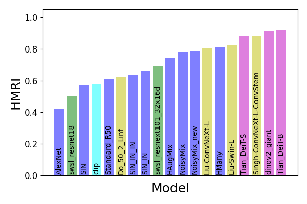
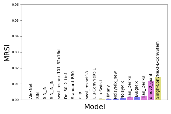
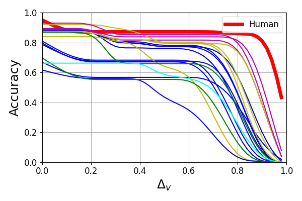
(a) HMRI for $\mathcal{R}_{a}$	(b) MRSI for $\mathcal{R}_{a}$	(c) Estimated curves $s_{a}$
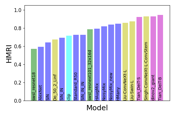
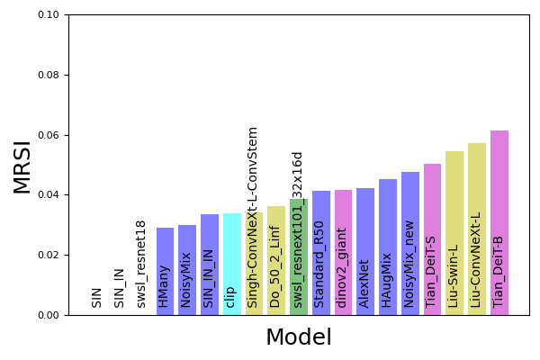
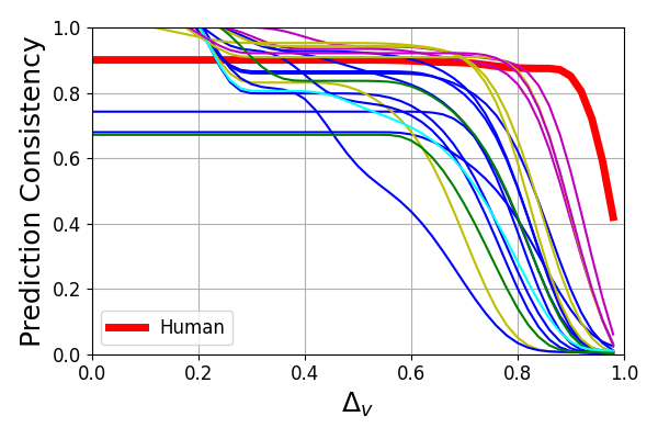
(d) HMRI for $\mathcal{R}_{p}$	(e) MRSI for $\mathcal{R}_{p}$	(f) Estimated curves $s_{p}$

Figure 23: VCR evaluation results for Shot Noise.

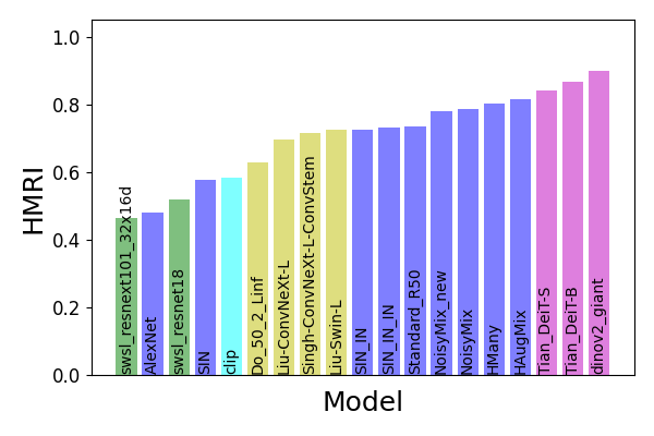
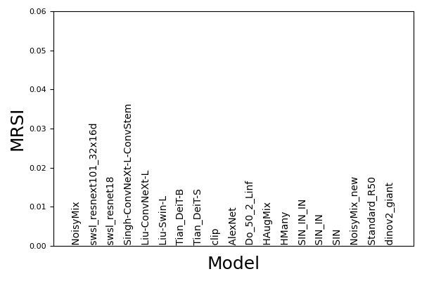
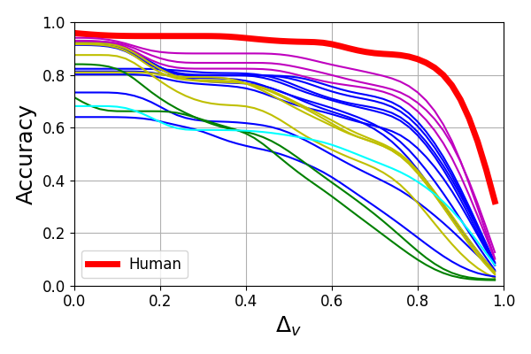
(a) HMRI for $\mathcal{R}_{a}$	(b) MRSI for $\mathcal{R}_{a}$	(c) Estimated curves $s_{a}$
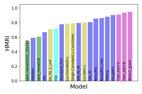
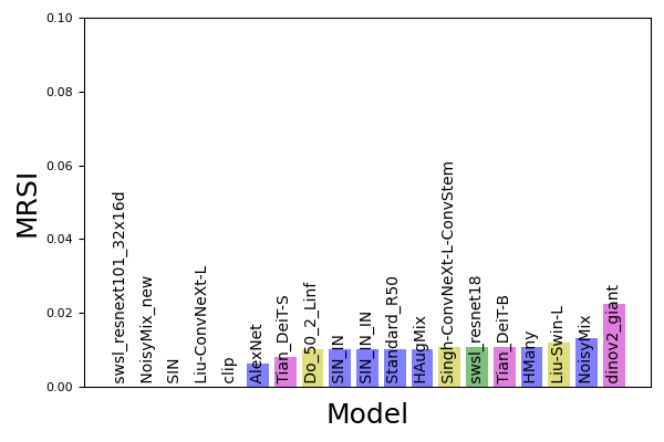
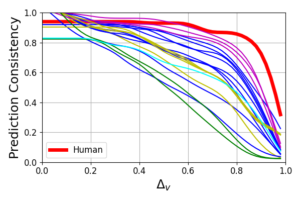
(d) HMRI for $\mathcal{R}_{p}$	(e) MRSI for $\mathcal{R}_{p}$	(f) Estimated curves $s_{p}$

Figure 24: VCR evaluation results for Blur.

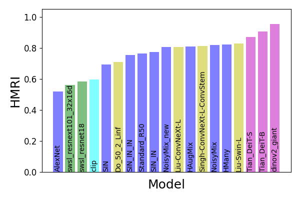
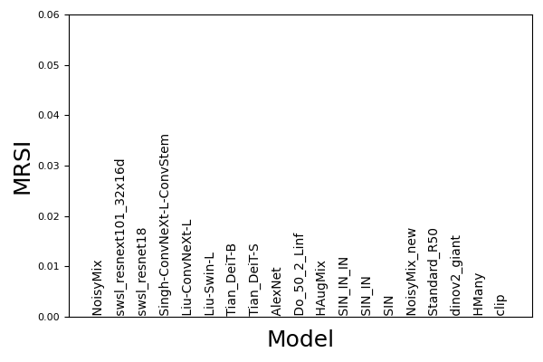
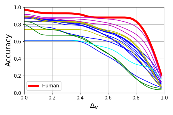
(a) HMRI for $\mathcal{R}_{a}$	(b) MRSI for $\mathcal{R}_{a}$	(c) Estimated curves $s_{a}$
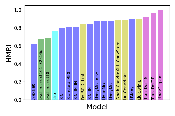
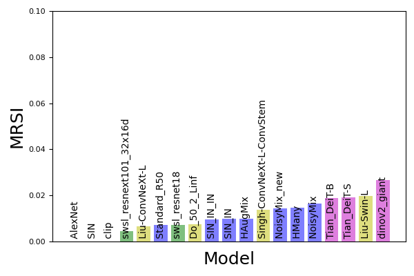
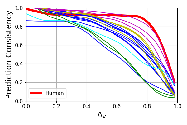
(d) HMRI for $\mathcal{R}_{p}$	(e) MRSI for $\mathcal{R}_{p}$	(f) Estimated curves $s_{p}$

Figure 25: VCR evaluation results for Median Blur.

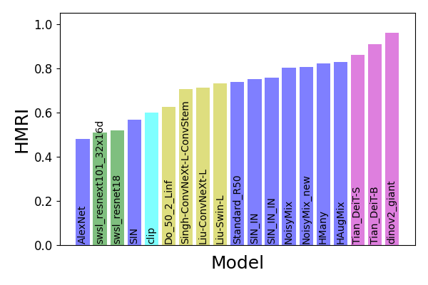
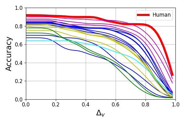
(a) HMRI for $\mathcal{R}_{a}$	(b) MRSI for $\mathcal{R}_{a}$	(c) Estimated curves $s_{a}$
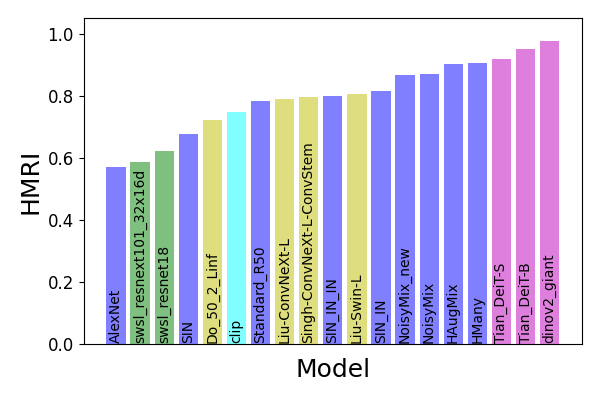
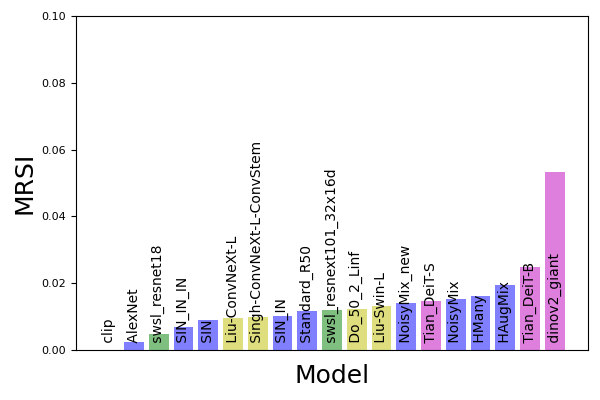
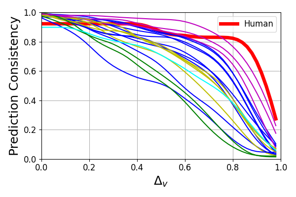
(d) HMRI for $\mathcal{R}_{p}$	(e) MRSI for $\mathcal{R}_{p}$	(f) Estimated curves $s_{p}$

Figure 26: VCR evaluation results for Glass Blur.

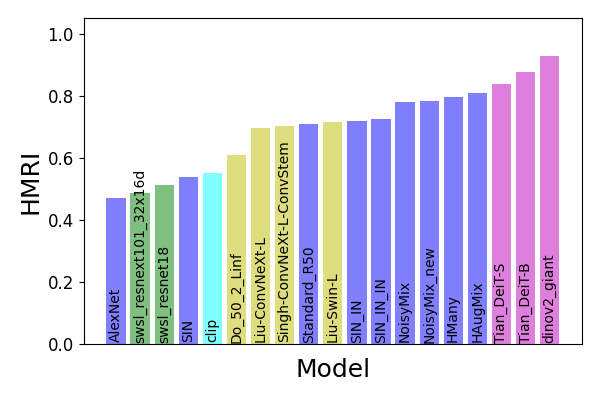
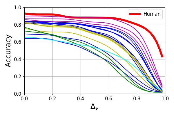
(a) HMRI for $\mathcal{R}_{a}$	(b) MRSI for $\mathcal{R}_{a}$	(c) Estimated curves $s_{a}$
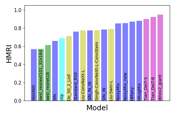
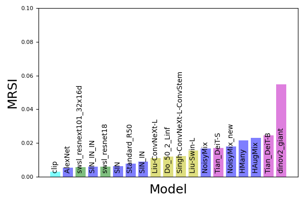
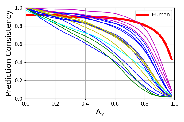
(d) HMRI for $\mathcal{R}_{p}$	(e) MRSI for $\mathcal{R}_{p}$	(f) Estimated curves $s_{p}$

Figure 27: VCR evaluation results for Gaussian Blur.

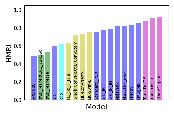
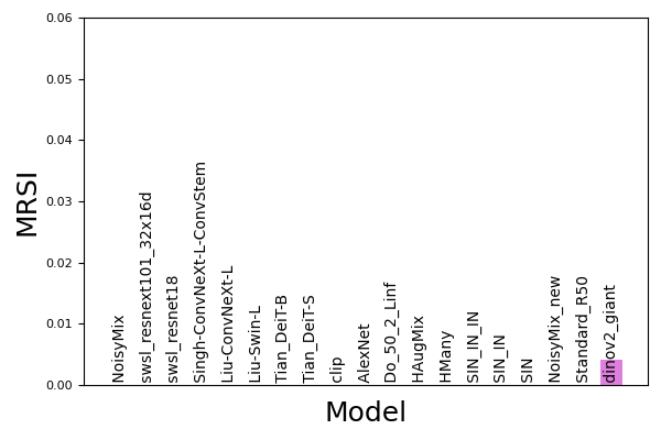
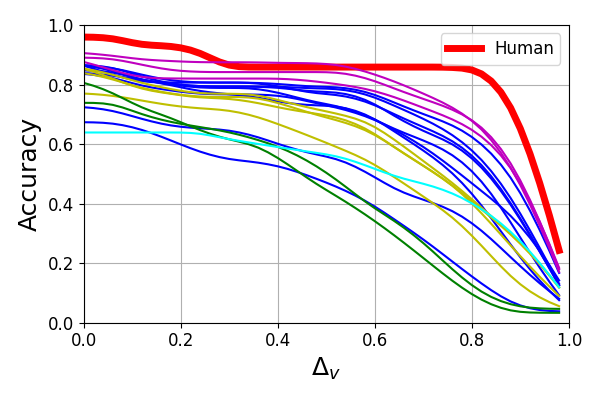
(a) HMRI for $\mathcal{R}_{a}$	(b) MRSI for $\mathcal{R}_{a}$	(c) Estimated curves $s_{a}$
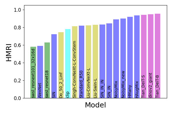
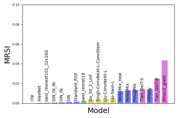
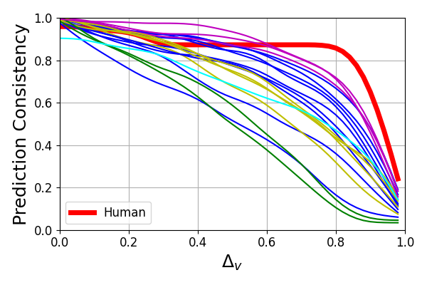
(d) HMRI for $\mathcal{R}_{p}$	(e) MRSI for $\mathcal{R}_{p}$	(f) Estimated curves $s_{p}$

Figure 28: VCR evaluation results for Defocus Blur.

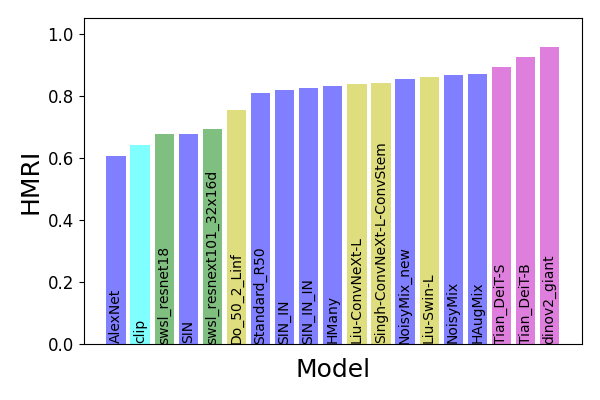
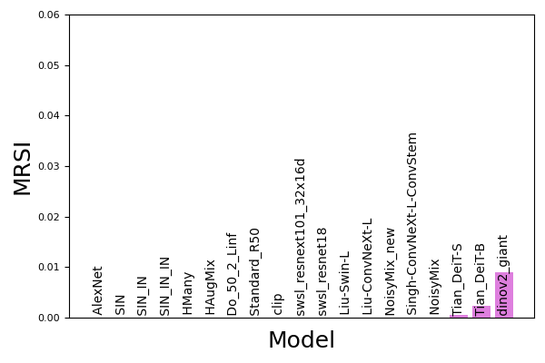
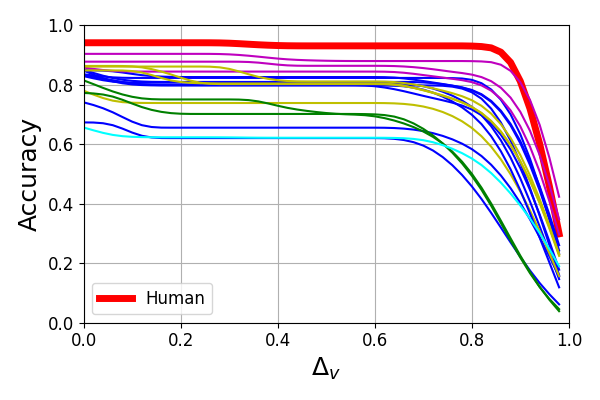
(a) HMRI for $\mathcal{R}_{a}$	(b) MRSI for $\mathcal{R}_{a}$	(c) Estimated curves $s_{a}$
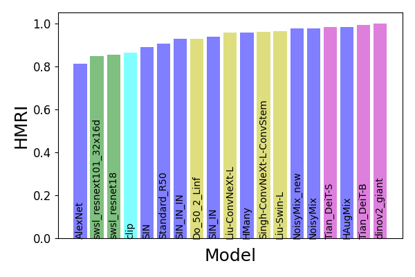
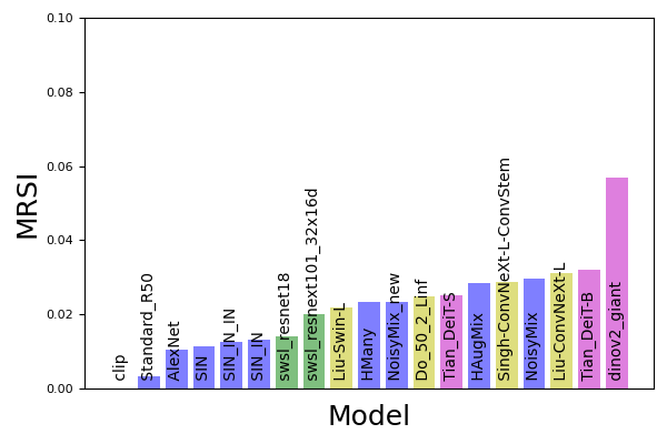
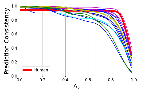
(d) HMRI for $\mathcal{R}_{p}$	(e) MRSI for $\mathcal{R}_{p}$	(f) Estimated curves $s_{p}$

Figure 29: VCR evaluation results for Motion Blur.

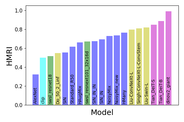
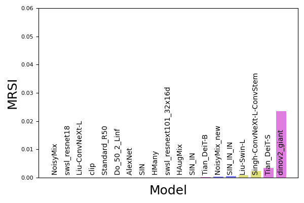
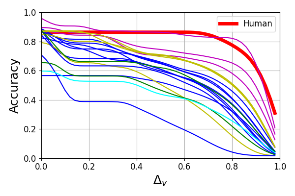
(a) HMRI for $\mathcal{R}_{a}$	(b) MRSI for $\mathcal{R}_{a}$	(c) Estimated curves $s_{a}$
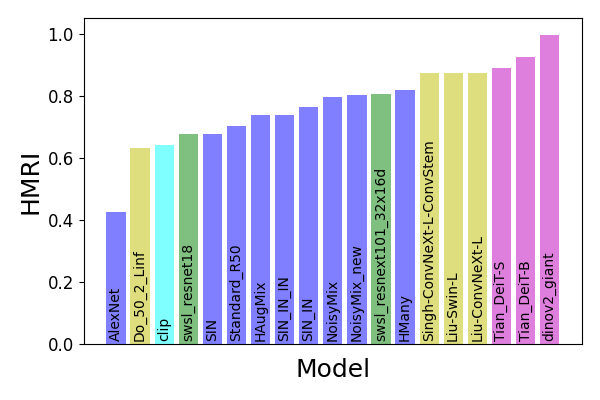
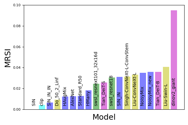
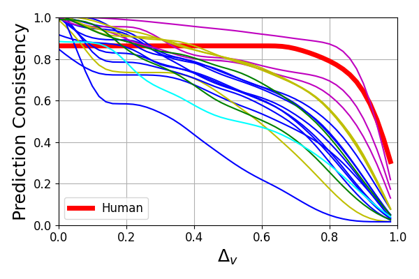
(d) HMRI for $\mathcal{R}_{p}$	(e) MRSI for $\mathcal{R}_{p}$	(f) Estimated curves $s_{p}$

Figure 30: VCR evaluation results for Hue Saturation Value.

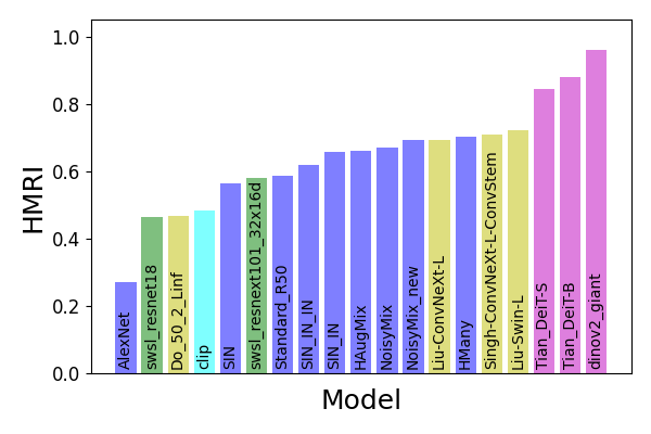
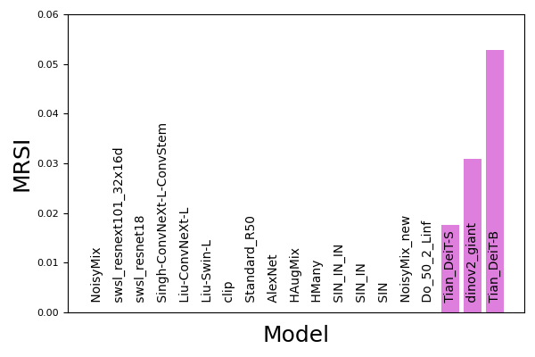
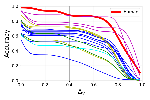
(a) HMRI for $\mathcal{R}_{a}$	(b) MRSI for $\mathcal{R}_{a}$	(c) Estimated curves $s_{a}$
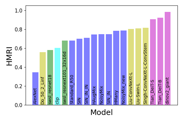
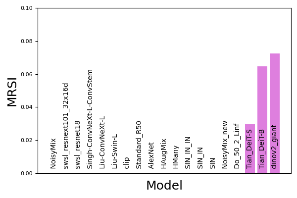
(d) HMRI for $\mathcal{R}_{p}$	(e) MRSI for $\mathcal{R}_{p}$	(f) Estimated curves $s_{p}$

Figure 31: VCR evaluation results for Color Jitter.

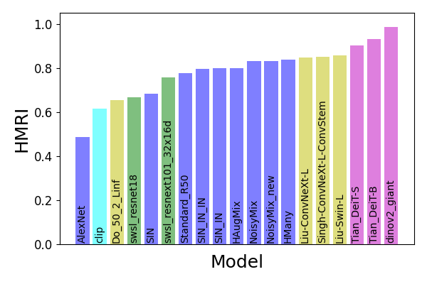
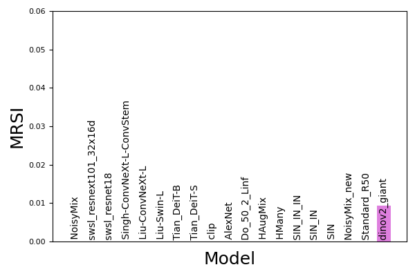
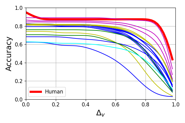
(a) HMRI for $\mathcal{R}_{a}$	(b) MRSI for $\mathcal{R}_{a}$	(c) Estimated curves $s_{a}$
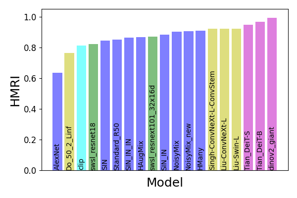
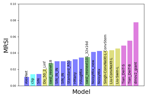
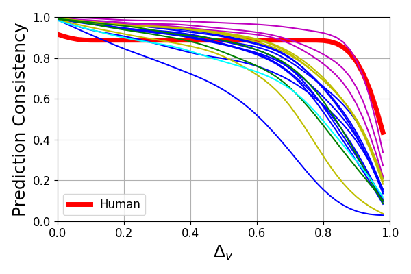
(d) HMRI for $\mathcal{R}_{p}$	(e) MRSI for $\mathcal{R}_{p}$	(f) Estimated curves $s_{p}$

Figure 32: VCR evaluation results for Brightness.

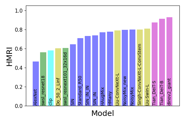
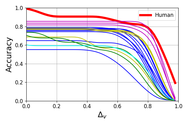
(a) HMRI for $\mathcal{R}_{a}$	(b) MRSI for $\mathcal{R}_{a}$	(c) Estimated curves $s_{a}$
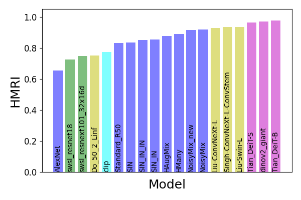
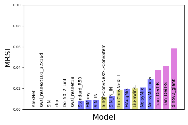
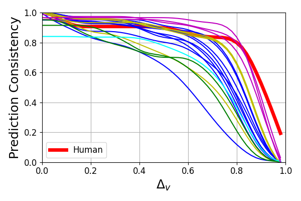
(d) HMRI for $\mathcal{R}_{p}$	(e) MRSI for $\mathcal{R}_{p}$	(f) Estimated curves $s_{p}$

Figure 33: VCR evaluation results for Frost.

References

- [1] Buslaev, A., Iglovikov, V.I., Khvedchenya, E., Parinov, A., Druzhinin, M., Kalinin, A.A.: Albumentations: Fast and Flexible Image Augmentations. Information 11(2) (2020). https://doi.org/10.3390/info11020125, licensed with MIT License. To view a copy of this license see https://github.com/albumentations-team/albumentations/blob/master/LICENSE.
- [2] Chattopadhyay, P., Hoffman, J., Mottaghi, R., Kembhavi, A.: RobustNav: Towards Benchmarking Robustness in Embodied Navigation. In: 2021 IEEE/CVF International Conference on Computer Vision, ICCV 2021, Montreal, QC, Canada, October 10-17, 2021. pp. 15671–15680. IEEE (2021). https://doi.org/10.1109/ICCV48922.2021.01540
- [3] Croce, F., Andriushchenko, M., Sehwag, V., Debenedetti, E., Flammarion, N., Chiang, M., Mittal, P., Hein, M.: RobustBench: A Standardized Adversarial Robustness Benchmark. In: Proceedings of the Neural Information Processing Systems Track on Datasets and Benchmarks 1, NeurIPS Datasets and Benchmarks 2021, December 2021, virtual (2021), https://robustbench.github.io/, licensed with MIT license. To view a copy of this license see https://github.com/RobustBench/robustbench/blob/master/LICENSE.
- [4] Ding, K., Ma, K., Wang, S., Simoncelli, E.P.: Image quality assessment: Unifying structure and texture similarity. IEEE Transactions on Pattern Analysis and Machine Intelligence 44(5), 2567–2581 (2022). https://doi.org/10.1109/TPAMI.2020.3045810
- [5] Erichson, N.B., Lim, S.H., Xu, W., Utrera, F., Cao, Z., Mahoney, M.W.: NoisyMix: Boosting Model Robustness to Common Corruptions (2022). https://doi.org/10.48550/ARXIV.2202.01263
- [6] Firestone, C.: Performance vs. Competence in Human–Machine Comparisons. Proceedings of the National Academy of Sciences 117(43), 26562–26571 (2020)
- [7] Geiger, A., Lenz, P., Stiller, C., Urtasun, R.: Vision Meets Robotics: The KITTI Dataset. Int. J. of Robotics Research (IJRR) (2013)
- [8] Geirhos, R., Medina Temme, C., Rauber, J., Schütt, H., Bethge, M., Wichmann, F.: Generalisation in Humans and Deep Neural Networks. In: NeurIPS 2018. pp. 7549–7561. Curran (2019)
- [9] Geirhos, R., Jacobsen, J., Michaelis, C., Zemel, R.S., Brendel, W., Bethge, M., Wichmann, F.A.: Shortcut learning in deep neural networks. Nat. Mach. Intell. 2(11), 665–673 (2020). https://doi.org/10.1038/s42256-020-00257-z
- [10] Geirhos, R., Narayanappa, K., Mitzkus, B., Thieringer, T., Bethge, M., Wichmann, F.A., Brendel, W.: Partial success in closing the gap between human and machine vision. In: Ranzato, M., Beygelzimer, A., Dauphin, Y.N., Liang, P., Vaughan, J.W. (eds.) Advances in Neural Information Processing Systems 34: Annual Conference on Neural Information Processing Systems 2021, NeurIPS 2021, December 6-14, 2021, virtual. pp. 23885–23899 (2021), https://proceedings.neurips.cc/paper/2021/hash/c8877cff22082a16395a57e97232bb6f-Abstract.html
- [11] Geirhos, R., Rubisch, P., Michaelis, C., Bethge, M., Wichmann, F.A., Brendel, W.: ImageNet-trained CNNs are Biased Towards Texture; Increasing Shape Bias Improves Accuracy and Robustness. In: 7th International Conference on Learning Representations, ICLR 2019, New Orleans, LA, USA, May 6-9, 2019 (2019)
- [12] He, K., Zhang, X., Ren, S., Sun, J.: Deep Residual Learning for Image Recognition. 2016 IEEE Conference on Computer Vision and Pattern Recognition (CVPR) pp. 770–778 (2016)
- [13] Hebart, M.N., Zheng, C.Y., Pereira, F., Baker, C.I.: Revealing the multidimensional mental representations of natural objects underlying human similarity judgements. Nature human behaviour 4(11), 1173–1185 (2020)
- [14] Hendrycks, D., Basart, S., Mu, N., Kadavath, S., Wang, F., Dorundo, E., Desai, R., Zhu, T., Parajuli, S., Guo, M., Song, D., Steinhardt, J., Gilmer, J.: The Many Faces of Robustness: A Critical Analysis of Out-of-Distribution Generalization. In: 2021 IEEE/CVF International Conference on Computer Vision, ICCV 2021, Montreal, QC, Canada, October 10-17, 2021. pp. 8320–8329. IEEE (2021). https://doi.org/10.1109/ICCV48922.2021.00823
- [15] Hendrycks, D., Dietterich, T.: Benchmarking Neural Network Robustness to Common Corruptions and Perturbations. Proceedings of the International Conference on Learning Representations (2019), https://github.com/hendrycks/robustness, licensed with Apache-2.0 license. To view a copy of this license see https://github.com/hendrycks/robustness/blob/master/LICENSE.
- [16] Hendrycks, D., Gimpel, K.: A Baseline for Detecting Misclassified and Out-of-Distribution Examples in Neural Networks. In: 5th International Conference on Learning Representations, ICLR 2017, Toulon, France, April 24-26, 2017, Conference Track Proceedings (2017)
- [17] Hendrycks, D., Mu, N., Cubuk, E.D., Zoph, B., Gilmer, J., Lakshminarayanan, B.: AugMix: A Simple Data Processing Method to Improve Robustness and Uncertainty. In: 8th International Conference on Learning Representations, ICLR 2020, Addis Ababa, Ethiopia, April 26-30, 2020 (2020)
- [18] Hendrycks, D., Zhao, K., Basart, S., Steinhardt, J., Song, D.: Natural Adversarial Examples. In: IEEE Conference on Computer Vision and Pattern Recognition, CVPR 2021, virtual, June 19-25, 2021. pp. 15262–15271. Computer Vision Foundation / IEEE (2021). https://doi.org/10.1109/CVPR46437.2021.01501
- [19] Ho-Phuoc, T.: CIFAR10 to Compare Visual Recognition Performance between Deep Neural Networks and Humans. ArXiv abs/1811.07270 (2018)
- [20] Hu, B.C., Marsso, L., Czarnecki, K., Salay, R., Shen, H., Chechik, M.: If a Human Can See It, So Should Your System: Reliability Requirements for Machine Vision Components. In: Proceedings of the 44th International Conference on Software Engineering (ICSE’2022), Pittsburgh, USA. ACM (2022)
- [21] Kamann, C., Rother, C.: Benchmarking the Robustness of Semantic Segmentation Models with Respect to Common Corruptions. Int. J. Comput. Vis. 129(2), 462–483 (2021). https://doi.org/10.1007/s11263-020-01383-2
- [22] Kar, O.F., Yeo, T., Atanov, A., Zamir, A.: 3D Common Corruptions and Data Augmentation. In: IEEE/CVF Conference on Computer Vision and Pattern Recognition, CVPR 2022, New Orleans, LA, USA, June 18-24, 2022. pp. 18941–18952. IEEE (2022). https://doi.org/10.1109/CVPR52688.2022.01839
- [23] Kheradpisheh, S.R., Ghodrati, M., Ganjtabesh, M., Masquelier, T.: Deep Networks Can Resemble Human Feed-forward Vision in Invariant Object Recognition. Scientific reports 6(1), 1–24 (2016)
- [24] Kim, B., Reif, E., Wattenberg, M., Bengio, S., Mozer, M.: Neural networks trained on natural scenes exhibit gestalt closure. arxiv. arXiv preprint arXiv:1903.01069 (2019)
- [25] Koenker, R., Ng, P., Portnoy, S.: Quantile Smoothing Splines. Biometrika 81(4), 673–680 (1994)
- [26] Krizhevsky, A., Sutskever, I., Hinton, G.E.: ImageNet Classification with Deep Convolutional Neural Networks. In: Advances in Neural Information Processing Systems 25: 26th Annual Conference on Neural Information Processing Systems 2012. Proceedings of a meeting held December 3-6, 2012, Lake Tahoe, Nevada, United States. pp. 1106–1114 (2012)
- [27] Kubilius, J., Schrimpf, M., Kar, K., Rajalingham, R., Hong, H., Majaj, N., Issa, E., Bashivan, P., Prescott-Roy, J., Schmidt, K., et al.: Brain-like object recognition with high-performing shallow recurrent anns. Advances in neural information processing systems 32 (2019)
- [28] Kumar, A.: Python 3 implementation of the visual information fidelity (vif) image quality assessment (iqa) metric. https://github.com/abhinaukumar/vif (2020), licensed with MIT license. To view a copy of this license see https://github.com/abhinaukumar/vif/blob/main/LICENSE.
- [29] Liu, C., Dong, Y., Xiang, W., Yang, X., Su, H., Zhu, J., Chen, Y., He, Y., Xue, H., Zheng, S.: A comprehensive study on robustness of image classification models: Benchmarking and rethinking (2023)
- [30] Lopes, R.G., Yin, D., Poole, B., Gilmer, J., Cubuk, E.D.: Improving robustness without sacrificing accuracy with patch gaussian augmentation. CoRR abs/1906.02611 (2019)
- [31] Madry, A., Makelov, A., Schmidt, L., Tsipras, D., Vladu, A.: Towards Deep Learning Models Resistant to Adversarial Attacks. In: 6th International Conference on Learning Representations, ICLR 2018, Vancouver, BC, Canada, April 30 - May 3, 2018, Conference Track Proceedings (2018)
- [32] Michaelis, C., Mitzkus, B., Geirhos, R., Rusak, E., Bringmann, O., Ecker, A.S., Bethge, M., Brendel, W.: Benchmarking Robustness in Object Detection: Autonomous Driving when Winter is Coming. arXiv preprint arXiv:1907.07484 (2019)
- [33] Mintun, E., Kirillov, A., Xie, S.: On Interaction Between Augmentations and Corruptions in Natural Corruption Robustness. In: Advances in Neural Information Processing Systems 34: Annual Conference on Neural Information Processing Systems 2021, NeurIPS 2021, December 6-14, 2021, virtual. pp. 3571–3583 (2021)
- [34] Oquab, M., Darcet, T., Moutakanni, T., Vo, H., Szafraniec, M., Khalidov, V., Fernandez, P., Haziza, D., Massa, F., El-Nouby, A., Assran, M., Ballas, N., Galuba, W., Howes, R., Huang, P.Y., Li, S.W., Misra, I., Rabbat, M., Sharma, V., Synnaeve, G., Xu, H., Jegou, H., Mairal, J., Labatut, P., Joulin, A., Bojanowski, P.: Dinov2: Learning robust visual features without supervision (2023)
- [35] Papadopoulos, D.P., Uijlings, J.R.R., Keller, F., Ferrari, V.: Training Object Class Detectors with Click Supervision. In: 2017 IEEE Conference on Computer Vision and Pattern Recognition, CVPR 2017, Honolulu, HI, USA, July 21-26, 2017. pp. 180–189. IEEE Computer Society (2017). https://doi.org/10.1109/CVPR.2017.27
- [36] Press, O., Schneider, S., Kümmerer, M., Bethge, M.: Rdumb: A simple approach that questions our progress in continual test-time adaptation (2023)
- [37] Radford, A., Kim, J.W., Hallacy, C., Ramesh, A., Goh, G., Agarwal, S., Sastry, G., Askell, A., Mishkin, P., Clark, J., Krueger, G., Sutskever, I.: Learning transferable visual models from natural language supervision (2021)
- [38] Rusak, E., Schott, L., Zimmermann, R.S., Bitterwolf, J., Bringmann, O., Bethge, M., Brendel, W.: Increasing the Robustness of DNNs Against Image Corruptions by Playing the Game of Noise. ArXiv abs/2001.06057 (2020)
- [39] Russakovsky, O., Deng, J., Su, H., Krause, J., Satheesh, S., Ma, S., Huang, Z., Karpathy, A., Khosla, A., Bernstein, M., Berg, A., Fei-Fei, L.: ImageNet Large Scale Visual Recognition Challenge. International Journal of Computer Vision 115, 211–252 (2015)
- [40] Salman, H., Ilyas, A., Engstrom, L., Kapoor, A., Madry, A.: Do Adversarially Robust ImageNet Models Transfer Better? In: Advances in Neural Information Processing Systems 33: Annual Conference on Neural Information Processing Systems 2020, NeurIPS 2020, December 6-12, 2020, virtual (2020)
- [41] Sheikh, H.R., Bovik, A.C.: Image Information and Visual Quality. IEEE Transactions on Image Processing 15(2), 430–444 (2006)
- [42] Sheikh, H.R., Sabir, M.F., Bovik, A.C.: A Statistical Evaluation of Recent Full Reference Image Quality Assessment Algorithms. IEEE Transactions on Image Processing 15(11), 3440–3451 (2006)
- [43] Singh, N.D., Croce, F., Hein, M.: Revisiting adversarial training for imagenet: Architectures, training and generalization across threat models (2023)
- [44] Stallkamp, J., Schlipsing, M., Salmen, J., Igel, C.: Man vs. Computer: Benchmarking Machine Learning Algorithms for Traffic Sign Recognition. Neural Networks 32, 323 – 332 (2012), selected Papers from IJCNN 2011
- [45] Storrs, K.R., Anderson, B.L., Fleming, R.W.: Unsupervised learning predicts human perception and misperception of gloss. Nature Human Behaviour 5(10), 1402–1417 (2021)
- [46] Sun, J., Zhang, Q., Kailkhura, B., Yu, Z., Xiao, C., Mao, Z.M.: Benchmarking Robustness of 3D Point Cloud Recognition Against Common Corruptions. CoRR abs/2201.12296 (2022)
- [47] Tian, R., Wu, Z., Dai, Q., Hu, H., Jiang, Y.G.: Deeper Insights into the Robustness of ViTs towards Common Corruptions (2022)
- [48] Wang, Z., Bovik, A., Sheikh, H., Simoncelli, E.: Image Quality Assessment: From Error Visibility to Structural Similarity. IEEE Trans. on Image Processing 13(4), 600–612 (2004)
- [49] Yalniz, I.Z., Jégou, H., Chen, K., Paluri, M., Mahajan, D.: Billion-scale semi-supervised learning for image classification. CoRR abs/1905.00546 (2019), http://arxiv.org/abs/1905.00546
- [50] Yamins, D.L., Hong, H., Cadieu, C.F., Solomon, E.A., Seibert, D., DiCarlo, J.J.: Performance-optimized hierarchical models predict neural responses in higher visual cortex. Proceedings of the national academy of Sciences 111(23), 8619–8624 (2014)
- [51] Yi, C., Yang, S., Li, H., Tan, Y., Kot, A.C.: Benchmarking the Robustness of Spatial-Temporal Models Against Corruptions. In: Proceedings of the Neural Information Processing Systems Track on Datasets and Benchmarks 1, NeurIPS Datasets and Benchmarks 2021, December 2021, virtual (2021)
- [52] Yin, D., Lopes, R.G., Shlens, J., Cubuk, E.D., Gilmer, J.: A Fourier Perspective on Model Robustness in Computer Vision. In: Advances in Neural Information Processing Systems 32: Annual Conference on Neural Information Processing Systems 2019, NeurIPS 2019, December 8-14, 2019, Vancouver, BC, Canada. pp. 13255–13265 (2019)
- [53] Yun, S., Han, D., Chun, S., Oh, S.J., Yoo, Y., Choe, J.: CutMix: Regularization Strategy to Train Strong Classifiers With Localizable Features. In: 2019 IEEE/CVF International Conference on Computer Vision, ICCV 2019, Seoul, Korea (South), October 27 - November 2, 2019. pp. 6022–6031. IEEE (2019). https://doi.org/10.1109/ICCV.2019.00612
- [54] Zhang, H., Cissé, M., Dauphin, Y.N., Lopez-Paz, D.: mixup: Beyond Empirical Risk Minimization. In: 6th International Conference on Learning Representations, ICLR 2018, Vancouver, BC, Canada, April 30 - May 3, 2018, Conference Track Proceedings (2018)
- [55] Zhang, R., Isola, P., Efros, A.A., Shechtman, E., Wang, O.: The unreasonable effectiveness of deep features as a perceptual metric. In: 2018 IEEE Conference on Computer Vision and Pattern Recognition, CVPR 2018, Salt Lake City, UT, USA, June 18-22, 2018. pp. 586–595. Computer Vision Foundation / IEEE Computer Society (2018). https://doi.org/10.1109/CVPR.2018.00068
- [56] Zhang, R., Isola, P., Efros, A.A., Shechtman, E., Wang, O.: The unreasonable effectiveness of deep features as a perceptual metric. In: 2018 IEEE/CVF Conference on Computer Vision and Pattern Recognition. pp. 586–595 (2018). https://doi.org/10.1109/CVPR.2018.00068