Verification of Neural Networks’ Global Robustness

Abstract.

Neural networks are successful in various applications but are also susceptible to adversarial attacks. To show the safety of network classifiers, many verifiers have been introduced to reason about the local robustness of a given input to a given perturbation. While successful, local robustness cannot generalize to unseen inputs. Several works analyze global robustness properties, however, neither can provide a precise guarantee about the cases where a network classifier does not change its classification. In this work, we propose a new global robustness property for classifiers aiming at finding the minimal globally robust bound, which naturally extends the popular local robustness property for classifiers. We introduce VHAGaR, an anytime verifier for computing this bound. VHAGaR relies on three main ideas: encoding the problem as a mixed-integer programming and pruning the search space by identifying dependencies stemming from the perturbation or network computation and generalizing adversarial attacks to unknown inputs. We evaluate VHAGaR on several datasets and classifiers and show that, given a three hour timeout, the average gap between the lower and upper bound on the minimal globally robust bound computed by VHAGaR is 1.9, while the gap of an existing global robustness verifier is 154.7. Moreover, VHAGaR is 130.6x faster than this verifier. Our results further indicate that leveraging dependencies and adversarial attacks makes VHAGaR 78.6x faster.

1. Introduction

Deep neural networks are successful in various tasks but are also susceptible to adversarial examples: malicious input perturbations designed to deceive the network. Many adversarial attacks target image classifiers and compute either an imperceptible change, bounded by a small $\epsilon$ with respect to an $L_{p}$ norm (e.g., $p=0,1,2,\infty$) (Chen et al., 2018; Carlini and Wagner., 2017; Chen et al., 2017; Madry et al., 2018; Zhang et al., 2020; Szegedy et al., 2014; Zhang et al., 2022b), or a perceivable change obtained by perturbing a semantic feature that does not change the semantics of the input, such as brightness, translation, or rotation (Bhattad et al., 2020; Engstrom et al., 2019, 2017; Wu et al., 2019; Liu et al., 2019).

A popular safety property for understanding a network’s robustness to such attacks is local robustness. Local robustness is parameterized by an input and its neighborhood. For a network classifier, the goal is to prove that the network classifies all inputs in the neighborhood the same. Several local robustness verifiers have been introduced for checking robustness in an $\epsilon$-ball (Tjeng et al., 2019; Singh et al., 2019b, a; Qin et al., 2019; Wang et al., 2018, 2021) or a feature neighborhood (Balunovic et al., 2019; Mohapatra et al., 2020). However, local robustness is limited to reasoning about a single neighborhood at a time. Thus, the network designer has to reason separately about every input that may arise in practice. This raises several issues. First, the space of inputs typically has a high dimensionality, making it impractical to be covered by a finite set of neighborhoods. Second, the robustness of a set of neighborhoods does not imply that unseen neighborhoods are robust. Third, even if the network designer can identify a finite set of relevant neighborhoods, existing local robustness verifiers take non-negligible time to reason about a single neighborhood. Thus, running them on a very large number of neighborhoods is impractical. Hence, local robustness does not enable to fully understand the robustness level of a network to a given perturbation for all inputs.

These issues gave rise to reasoning about a network’s robustness over all possible inputs, known as global robustness. Several works analyze global robustness properties. They can be categorized into two primary groups: precise analysis (Katz et al., 2017, 2019; Wang et al., 2022a, b) and sampling-based analysis (Ruan et al., 2019; Bastani et al., 2016; Mangal et al., 2019; Levy et al., 2023). Existing precise analysis techniques focus primarily on the $L_{\infty}$ $\epsilon$-ball and a global robustness property defined over the network’s stability (Wang et al., 2022a, b; Katz et al., 2017). The network’s stability is the maximum difference of the output vectors of an input and a perturbed example in that input’s $\epsilon$-ball. This approach cannot capture the desired robustness property for classifiers, which is that the inputs’ classification does not change under a given perturbation. The second kind of analyzers computes a probabilistic global robustness bound by analyzing the local robustness of samples from the input space (Mangal et al., 2019; Levy et al., 2023) or a given dataset (Ruan et al., 2019; Bastani et al., 2016). Sampling-based analyzers scale better than the precise analyzers but only provide a lower bound on the actual global robustness bound.

In this work, we propose a new global robustness property designated for classifiers, which is general to any perturbation such as the $L_{\infty}$ perturbation or feature perturbations. Intuitively, a classifier is globally robust to a given perturbation if for any input for which the network is confident enough in its classification, this perturbation does not cause the network to change its classification. We focus on such inputs because it is inevitable that inputs near the decision boundaries, where the network’s classification confidence is low, are misclassified when adding perturbations. Note that, like previous works (Katz et al., 2017, 2019; Wang et al., 2022a, b), our global robustness property considers any input, including meaningful inputs and meaningless noise. In a scenario where the focus is only on meaningful inputs, our property can theoretically be restricted to this space. However, this requires a formal characterization of the meaningful input space, which is generally nonexistent. For such scenario, our property, which considers any input, can be viewed as over-approximating the space of meaningful inputs for which the network is confident enough.

We address the problem of computing the minimal globally robust bound of a given network and perturbation. Namely, any input that the network classifies with a confidence that is at least this bound is not misclassified under this perturbation. Although our global robustness property is not the first to consider any input, it is the first to consider the classifier’s minimal bound satisfying global robustness. This difference is similar to the difference between verifying local robustness at a given $\epsilon$-ball (e.g., like Tjeng et al. (2019); Singh et al. (2019b)) and computing the maximal $\epsilon$-ball which is locally robust (e.g., like Kabaha and Drachsler-Cohen (2023)). Our problem is highly challenging for two main reasons. First, it is challenging to determine for a given confidence whether a classifier is globally robust since it requires to determine the robustness of a very large space of unknown inputs; even local robustness verification, reasoning about a single input’s neighborhood, is under active research. Second, our problem requires to compute the minimal globally robust bound, and thus it requires reasoning about the global robustness over a large number of confidences.

We introduce VHAGaR, a Verifier of Hazardous Attacks for proving Global Robustness that computes the minimal globally robust bound of a network classifier, under a given perturbation. VHAGaR relies on three key ideas. First, it encodes the problem as a mixed-integer programming (MIP), enabling efficient optimization through existing MIP solvers. Further, VHAGaR is designed as an anytime algorithm and asks the MIP solver to compute a lower and an upper bound on the minimal globally robust bound. Second, it prunes the search space by computing dependencies stemming from the perturbation or the network computation. Third, it executes a hyper-adversarial attack, generalizing adversarial attacks to unknown inputs, to efficiently compute suboptimal lower bounds on the robustness bound that further prune the search space. Our attack also identifies optimization hints, partial assignments to the MIP’s variables, guiding towards the optimal solution. VHAGaR currently supports the $L_{\infty}$ perturbation and six semantic feature perturbations (Figure 1(a)).

Figure 1. (a) The perturbations supported by VHAGaR. (b) VHAGaR’s upper and lower bounds on the minimal globally robust bound vs. sampling approaches, Marabou and a MIP-only variant of VHAGaR.

We evaluate VHAGaR on several fully-connected and convolutional image classifiers, trained for MNIST, Fashion-MNIST and CIFAR-10. We compare to existing approaches, including Marabou (Katz et al., 2019) and sampling-based approaches: Dataset Sampling, relying on a dataset, and Random Sampling, sampling from the input domain. We further show the importance of integrating the dependencies and hyper-adversarial attacks by comparing them to a MIP-only variant of VHAGaR. Our results show that (1) the average gap between the lower and upper bound of VHAGaR is 1.9, while Marabou’s gap is 154.7, (2) the lower bound of VHAGaR is greater (i.e., tighter) by 6.5x than Marabou, by 9.2x than Dataset Sampling and by 25.6x than Random Sampling, (3) the upper bound of VHAGaR is smaller (i.e., tighter) by 13.1x than Marabou, and (4) VHAGaR is 130.6x faster than Marabou. Our results further indicate that VHAGaR is 78.6x faster than the MIP-only variant. Figure 1(b) shows our results for an MNIST convolutional network, classifying images to digits, and an occlusion perturbation, blackening a 3x3 square at the center of the image. The goal of this experiment is to compute the minimal globally robust bound for which any input that the network classifies as the digit 2 with a confidence over this bound cannot be perturbed by this occlusion such that the network classifies it as the digit 3. The plot shows that, given a three hour timeout, VHAGaR returns the optimal minimal bound (the lower and upper bound are equal), while the gap of the MIP-only variant is 10.1 and the gap of Marabou is 86.6. The sampling baselines, providing only a lower bound, return a bound lower than the minimal bound by 3x. Figure 1(b) highlights in a light blue background the range of confidences for which every approach proves global robustness, and in a light red background the range of confidences for which every approach guarantees there is no global robustness. VHAGaR perfectly partitions this range, while the other approaches leave a range of confidences without any guarantee. We further experimentally show how to leverage VHAGaR’s computed bounds to infer global robustness and vulnerability attributes of the network.

2. Preliminaries

In this section, we provide background on network classifiers. We focus on image classifiers. An image is a $d_{1}\times d_{2}$ matrix, where $d_{1}$ is the height and $d_{2}$ is the width. The entries are pixels consisting of $l$ channels, each over $[0,1]$. If $l=1$, the image is in grayscale, if $l=3$, it is colored (RGB). Given an image domain $[0,1]^{l\times d_{1}\times d_{2}}$ and a set of classes $C=\{1,\dots,c\}$, a classifier maps images to a score vector over the possible classes $D:[0,1]^{l\times d_{1}\times d_{2}}\to\mathbb{R}^{c}$. We assume a non-trivial classifier, that is $c>1$ and for any class $c^{\prime}\in C$ there is an input classified as $c^{\prime}$. A neural network classifier consists of an input layer followed by $L$ layers. For simplicity’s sake, our definitions treat all layers as vectors, except where the definition requires a matrix. The input layer $z_{0}$ takes as input an image $x$ and passes it to the next layer (i.e., $z_{0,k}=x_{k}$). The last layer outputs a vector, denoted $D(x)$, consisting of a score for each class in $C$. The classification of the network for input $x$ is the class with the highest score, $c^{\prime}=\text{argmax}(D(x))$. The layers are functions, denoted $h_{1},h_{2},\dots,h_{L}$, each taking as input the output of the preceding layer. The network’s function is the composition of the layers: $D(x)=h_{L}(h_{L-1}(\cdots(h_{1}(x))))$. A layer $m$ consists of $k_{m}$ neurons, denoted $z_{m,1},\ldots,z_{m,k_{m}}$. The function of layer $m$ is defined by its neurons, i.e., it outputs the vector $(z_{m,1},\ldots,z_{m,k_{m}})^{T}$. There are several types of layers. We focus on fully-connected and convolutional layers, but our approach is easily extensible to other layers such as max pooling layers and residual layers (He et al., 2016).

In a fully-connected layer, a neuron $z_{m,k}$ gets as input the outputs of all neurons in the preceding layer. It has a weight for each input ${w}_{m,k,k^{\prime}}$ and a single bias $b_{m,k}$. Its function is computed by first computing the sum of the bias and the multiplication of every input by its respective weight: $\hat{z}_{m,k}=b_{m,k}+\sum_{k^{\prime}=1}^{k_{m-1}}{w}_{m,k,k^{\prime}}\cdot{z}_{m-1,k^{\prime}}$. This output is passed to an activation function $\sigma$ to produce the output $z_{m,k}=\sigma(\hat{z}_{m,k})$. Activation functions are typically non-linear functions. We focus on ReLU, defined as $\text{ReLU}(\hat{z})=\max(0,\hat{z})$. A convolutional layer is similar to a fully-connected layer except that a neuron does not get as input all neurons from the preceding layer, but only a small subset of them. Additionally, neurons at the same layer share their weights and bias. The set of shared weights and bias are collectively called a kernel. Formally, a convolutional layer views its input as a matrix $l\times d^{h}_{m-1}\times d^{w}_{m-1}$, where $l$ is the number of input channels, $d^{h}_{m-1}$ is the height and $d^{w}_{m-1}$ is the width. A kernel $K$ consists of a weight matrix $W_{m}$ of dimension $l\times t_{m}\times t_{m}$ and a bias $b_{m}$. A kernel is convolved with the input $\hat{z}_{m,l,i,j}=b_{m}+\sum_{v=1}^{l}\sum^{t_{m}}_{p=1}\sum^{t_{m}}_{q=1}W[v,p,q]\cdot z_{m-1,v,p,q}$, after which an activation function (e.g., ReLU) is executed component-wise.

3. Minimal Globally Robust Bounds

In this section, we present our global robustness property designated for network classifiers. We begin with a few definitions and then define our property and the problem we address.

Perturbations

A perturbation is a function $f_{P}(x,\mathcal{E})$, defining how an input $x$ is perturbed given an amount of perturbation specified by a vector $\mathcal{E}=(\epsilon_{1},\ldots,\epsilon_{k})$. The perturbation values $\epsilon_{i}$ are either real numbers or integers. For example, brightness is defined by a brightness level $\epsilon\in[-1,1]$ and the function is $f_{B}(x,\epsilon)=x^{\prime}$ such that $x^{\prime}_{v,p,q}=x_{v,p,q}+\epsilon$, for $v\in[l]$, $p\in[d_{1}]$, $q\in[d_{2}]$. Translation is defined by translation coordinates $i\in[-d_{1},d_{1}]$ and $j\in[-d_{2},d_{2}]$ and the function is $f_{T}(x,i,j)=x^{\prime}$ such that $x^{\prime}_{v,p,q}=(p-i\in[d_{1}]\wedge q-j\in[d_{2}]?\ x_{v,p-i,q-j}\ :\ 0)$. The $L_{\infty}$ perturbation has a perturbation limit $\epsilon\in[0,1]$ and is defined by a series of perturbations $\epsilon_{v,p,q}\in[-\epsilon,\epsilon]$, for $v\in[l]$, $p\in[d_{1}]$, $q\in[d_{2}]$. The function is $f_{L_{\infty}}(x,\epsilon_{1,1,1},\ldots,\epsilon_{l,d_{1},d_{2}})=x^{\prime}$ such that $x^{\prime}_{v,p,q}=x_{v,p,q}+\epsilon_{v,p,q}$. We note that if a perturbed entry is not in its valid range (i.e., below $0$ or above $1$), it is clipped: $\min(\max(f_{P}(x,\mathcal{E})_{v,p,q},0),1)$. We omit clipping from the formal definitions to avoid a cluttered notation. A perturbation is confined by a range $I_{\mathcal{E}}$, a series of intervals bounding each entry of $\mathcal{E}$. For example, a range for brightness is $[0.1,0.3]\subseteq[-1,1]$, bounding the values of the brightness level $\epsilon$, and a range for translation is $([1,3],[2,10])\subseteq([-d_{1},d_{1}],[-d_{2},d_{2}])$ (for $d_{1}\geq 3,d_{2}\geq 10$), bounding the coordinates $i$ and $j$. An amount of perturbation $\mathcal{E}^{\prime}$ is in a given range $I_{\mathcal{E}}$, denoted $\mathcal{E}^{\prime}\in I_{\mathcal{E}}$, if its entries are in their intervals: $\forall k.\ \mathcal{E}^{\prime}_{k}\in(I_{\mathcal{E}})_{k}$. For example, $(2,4)\in([1,3],[2,10])$.

Local robustness

A common approach to estimate the robustness of a classifier focuses on a finite set of inputs and checks local robustness for every input, one-by-one. Local robustness is checked at a given neighborhood, defined with respect to an input and a perturbation. Formally, given an input $x$, a perturbation $P$ and its range $I_{\mathcal{E}}$, a neighborhood $\mathcal{N}_{P,I_{\mathcal{E}}}(x)\subseteq[0,1]^{l\times d_{1}\times d_{2}}$ is the set of all inputs obtained by this perturbation: $\mathcal{N}_{P,I_{\mathcal{E}}}(x)=\{f_{P}(x,\mathcal{E}^{\prime})\mid\mathcal{E}^{\prime}\in I_{\mathcal{E}}\}$. Given a classifier $D$, an input $x$ and a neighborhood containing $x$, $\mathcal{N}_{P,I_{\mathcal{E}}}(x)\subseteq[0,1]^{l\times d_{1}\times d_{2}}$, the classifier $D$ is locally robust at $\mathcal{N}_{P,I_{\mathcal{E}}}(x)$ if it classifies all inputs the same: $\forall x^{\prime}\in\mathcal{N}_{P,I_{\mathcal{E}}}(x).\ \text{argmax}(D(x^{\prime}))=\text{argmax}(D(x))$. Equivalently, $D$ is locally robust at $x$ under $P$ and $I_{\mathcal{E}}$ if $\forall\mathcal{E}^{\prime}\in I_{\mathcal{E}}.\ \text{argmax}(D(f_{P}(x,\mathcal{E}^{\prime})))=\text{argmax}(D(x))$.

Towards a global robustness property

Given a perturbation $P$ and its range $I_{\mathcal{E}}$, an immediate extension of the local robustness definition to global robustness is:

$$\forall x\forall\mathcal{E}^{\prime}\in I_{\mathcal{E}}.\ \text{argmax}(D(f_{P}(x,\mathcal{E}^{\prime})))=\text{argmax}(D(x))$$

However, no (non-trivial) network classifier satisfies this property because some inputs $x$ are close to the classifier’s decision boundaries (Alfarra et al., 2020; Huang, 2020) and violate this property. We thus consider only inputs whose network’s confidence is high enough and thus are far enough from the decision boundaries. Formally, the network’s confidence in classifying an input $x$ as a class $c^{\prime}\in\{1,\ldots,c\}$ is the difference between the score the network assigns to $c^{\prime}$ and the maximal score it assigns to any other class. If this confidence is positive, the network classifies $x$ as $c^{\prime}$, and the higher the (positive) number, the more certain the network is in its classification of $x$ as $c^{\prime}$.

Definition 3.1 (Class Confidence).

Given a classifier $D$, an input $x$ and a class $c^{\prime}$, the class confidence of $D$ in $c^{\prime}$ is $\mathcal{C}(x,c^{\prime},D)\triangleq D(x)_{c^{\prime}}-\text{max}_{c^{\prime\prime}\neq c^{\prime}}(D(x)_{c^{\prime\prime}})$.

$\delta$-Global Robustness

We define global robustness with respect to a confidence level $\delta$. The definition restricts the above definition to inputs whose class confidence is at least $\delta$.

Definition 3.2 ($\delta$-Globally Robust Classifier).

Given a classifier $D$, a class $c^{\prime}\in[c]$, a perturbation ${P}$, a range $I_{\mathcal{E}}$ and a class confidence $\delta>0$, the classifier $D$ is $\delta$-globally robust for $c^{\prime}$ under $(P,I_{\mathcal{E}})$ if:

$$\forall x\forall\mathcal{E}^{\prime}\in I_{\mathcal{E}}.\ \mathcal{C}(x,c^{\prime},D)\geq\delta\Rightarrow\text{argmax}(D(f_{P}(x,\mathcal{E}^{\prime})))=\text{argmax}(D(x))$$

The postcondition $\text{argmax}(D(f_{P}(x,\mathcal{E}^{\prime})))=\text{argmax}(D(x))$ is equivalent to $\mathcal{C}(f_{P}(x,\mathcal{E}^{\prime}),c^{\prime},D)>0$, whenever the precondition $\mathcal{C}(x,c^{\prime},D)\geq\delta$ holds. We thus use these constraints interchangeably. When it is clear from the context, we write $D$ is $\delta$-globally robust and omit $c^{\prime}$ and $(P,I_{\mathcal{E}})$. The parameter $\delta$ in the precondition provides the necessary flexibility. The higher the $\delta$, the fewer inputs that are considered and the more likely that the classifier is globally robust with respect to that $\delta$. To understand the global robustness level of a classifier, one has to compute the minimal $\delta$ for which the classifier is globally robust. This is the problem we address, which we next define.

Definition 3.3 (Minimal Globally Robust Bound).

Given a classifier $D$, a class $c^{\prime}$, a perturbation ${P}$ and a range $I_{\mathcal{E}}$, our goal is to compute a class confidence $\delta_{\text{MIN}}\in\mathbb{R}^{+}$ satisfying: (1) $D$ is $\delta_{\text{MIN}}$-globally robust for $c^{\prime}$ under $(P,I_{\mathcal{E}})$, and (2) for every $\delta<\delta_{\text{MIN}}$, $D$ is not $\delta$-globally robust for $c^{\prime}$ under $(P,I_{\mathcal{E}})$.

This problem is highly challenging for two reasons. First, determining for a given $\delta$ whether a classifier $D$ is $\delta$-globally robust for $c^{\prime}$ under $(P,I_{\mathcal{E}})$ (for non-trivial $\delta$, $D$, $P$ and $I_{\mathcal{E}}$) requires to determine whether $D$ classifies a very large space of inputs as $c^{\prime}$. Second, to determine the minimal confidence $\delta_{\text{MIN}}$ for which $D$ is $\delta_{\text{MIN}}$-globally robust for $c^{\prime}$ under $(P,I_{\mathcal{E}})$ requires to determine for a large set of $\delta$ values whether $D$ is $\delta$-globally robust for $c^{\prime}$ under $(P,I_{\mathcal{E}})$.

Targeted global robustness

The above definitions aim to show that the network does not change its classification under a given perturbation. In some scenarios, network designers may permit some class changes. For example, they may allow the network to misclassify a perturbed dog as a cat, but not as a truck. Thus, when determining global robustness, it is sometimes more useful to guarantee that the network does not change its classification to a target class, rather than to any class but the correct class. We next adapt our definitions to targeted global robustness.

Definition 3.4 ($\delta$-Targeted Globally Robust Classifier).

Given a classifier $D$, a class $c^{\prime}\in[c]$, a target class $c_{t}\in[c]$ such that $c_{t}\neq c^{\prime}$, a perturbation ${P}$, a range $I_{\mathcal{E}}$ and a class confidence $\delta>0$, the classifier $D$ is $\delta$-globally robust against $c_{t}$ under $(P,I_{\mathcal{E}})$ if:

$$\forall x\forall\mathcal{E}^{\prime}\in I_{\mathcal{E}}.\ \mathcal{C}(x,c^{\prime},D)\geq\delta\Rightarrow\text{argmax}(D(f_{P}(x,\mathcal{E}^{\prime})))\neq c_{t}$$

The problem definition of computing the minimal targeted globally robust bound for a target class $c_{t}$ is the same as Definition 3.3 but with respect to Definition 3.4. Note that computing the minimal globally robust bound for $c^{\prime}$ can be obtained by computing the maximum minimal targeted globally robust bounds of all classes, except $c^{\prime}$. In the next section, we continue with the untargeted definition (Definition 3.3), but all definitions and algorithms easily adapt to the targeted definition.

4. Overview of Key Ideas

In this section, we present our main ideas to compute the minimal globally robust bound. We begin by introducing the straightforward optimization formalism for our problem and explaining why it is not amenable to standard MIP solvers. Then, we introduce the key components of VHAGaR. First, we rephrase the optimization problem into a form supported by MIP solvers, which also enables VHAGaR an anytime optimization (Figure 2). The anytime computation splits the problem into computing an upper bound and a lower bound for the minimal globally robust bound. Second, we identify dependencies that reduce the time complexity of solving the optimization problem (Section 4.2). Third, we compute a suboptimal lower bound and optimization hints, using a hyper-adversarial attack, which are provided to the MIP solver to expedite the tightening of the bounds (Section 4.3). Figure 2 demonstrates the importance of our steps. This figure shows the upper and lower bounds obtained by the anytime optimization as a function of the time, for a convolutional network composed of 540 neurons trained for the MNIST dataset and an occlusion perturbation. Figure 2(a) shows the bounds obtained by our encoding (Figure 2). While the bounds are tightened given more time, their gap is quite large after ten minutes. Figure 2(b) shows the improvement obtained by encoding the dependencies (Section 4.2): the bounds are tightened more significantly and more quickly. Figure 2(c) shows the improvement obtained by additionally providing the suboptimal lower bound and the optimization hints (Section 4.3): the lower and upper bounds are tightened more quickly and converge to the minimal globally robust bound within 72 seconds.

4.1. Minimal Globally Robust Bound via Optimization

Figure 2. The bounds vs. the execution time, when providing a MIP solver (a) our encoding, (b) additionally providing dependencies, and (c) additionally providing a suboptimal lower bound and optimization hints.

In this section, we phrase the problem of minimal globally robust bound as constrained optimization. Phrasing a problem as constrained optimization and providing it to a suitable solver has been shown to be very efficient in solving complex search problems and in particular robustness-related tasks, such as computing adversarial examples (Szegedy et al., 2014; Carlini and Wagner., 2017; Chen et al., 2017; Madry et al., 2018) and proving local robustness (Tjeng et al., 2019; Singh et al., 2019c, a; Wang et al., 2021). However, the straightforward formulation of our task, building on the aforementioned tasks, is not amenable to existing MIP solvers. We thus present an equivalent formulation, amenable to these solvers. We begin with the straightforward formulation and then show the equivalent formulation. The straightforward formulation follows directly from Definition 3.3:

Problem 1 (Minimal Globally Robust Bound).

Given a classifier $D$, a class $c^{\prime}$, a perturbation $P$ and a range $I_{\mathcal{E}}$, the constrained optimization computing the minimal globally robust bound is:

(1) $$\begin{gathered}\min\delta\hskip 7.11317pt\text{subject to}\hskip 7.11317pt\forall x\forall\mathcal{E}^{\prime}\in I_{\mathcal{E}}.\ \mathcal{C}(x,c^{\prime},D)\geq\delta\Rightarrow\mathcal{C}(f_{P}(x,\mathcal{E}^{\prime}),c^{\prime},D)>0\end{gathered}$$

This constraint requires that for any input classified as $c’$ with confidence over $\delta$, its perturbations are classified as $c’$. The optimal solution $\delta^{*}_{(1)}$ ranges over $[\Delta,\delta^{m}_{c^{\prime}}+\Delta]$, where $\delta^{m}_{c^{\prime}}$ is the maximal confidence that the classifier $D$ assigns to $c^{\prime}$ for any input (i.e., $\delta^{m}_{c^{\prime}}=\max_{x}\;\mathcal{C}(x,c^{\prime},D)$) and $\Delta$ is a very small number that denotes the computer’s precision level for representing the real numbers. For example, if the perturbation is the identity function, then $\delta^{*}_{(1)}=\Delta$. More generally, if the perturbation does not lead $D$ to change the classification, then $\delta^{*}_{(1)}=\Delta$. If the perturbation can perturb every pixel within its range $[0,1]$, then $\delta^{*}_{(1)}=\delta^{m}_{c^{\prime}}+\Delta$. In this case, the right-hand side of the constraint pertains to every input (i.e., for every $x^{\prime}\in[0,1]^{l\times d_{1}\times d_{2}}$ there is $\mathcal{E}^{\prime}$ such that $f_{P}(x,\mathcal{E^{\prime}})=x^{\prime}$). Since we assume $D$ classifies inputs to at least two classes ($c>1$), every input $x$ violates the postcondition because there are inputs $x^{\prime}$ not classified as $c^{\prime}$. Namely, $\delta^{m}_{c^{\prime}}$ is the maximal value for which the postcondition does not hold. Since for $\delta^{m}_{c^{\prime}}+\Delta$ the precondition is vacuously true, $\delta^{*}_{(1)}=\delta^{m}_{c^{\prime}}+\Delta$ is the minimal value satisfying the constraint of Problem 1. For other (more interesting) perturbations, $\delta^{*}_{(1)}\in(\Delta,\delta^{m}_{c^{\prime}}+\Delta)$ (note that $\delta^{m}_{c^{\prime}}$ depends on $D$).

Problem 1 cannot be submitted to existing MIP solvers, because its constraint has a for-all operator defined over a continuous range. Instead, we consider the dual problem: computing the maximal globally non-robust bound. This problem looks for the maximal ${\delta}$ violating the constraint of Problem 1. Namely, for every $\delta^{\prime}\geq{\delta}$ the network is $\delta^{\prime}$-globally robust, and for every $\delta^{\prime}<{\delta}$ there is an input $x$ and a perturbation amount $\mathcal{E}^{\prime}$ for which the network is not robust. Formally:

Problem 2 (Maximal Globally Non-Robust Bound).

(2) $$\begin{gathered}\max\delta\hskip 7.11317pt\text{subject to}\hskip 7.11317pt\exists x\exists\mathcal{E}^{\prime}\in I_{\mathcal{E}}.\ \mathcal{C}(x,c^{\prime},D)>\delta\wedge\mathcal{C}(f_{P}(x,\mathcal{E}^{\prime}),c^{\prime},D)\leq 0\end{gathered}$$

By definition, the optimal solution $\delta^{*}_{(2)}$ ranges over $[0,\delta^{m}_{c^{\prime}}]$. In the special case where the perturbation does not lead $D$ to change its classification, i.e., $\delta^{*}_{(1)}=\Delta$, then Problem 2 is infeasible. For completeness of the definition, in this case, we define $\delta^{*}_{(2)}\triangleq 0$. Note that Problem 1 and Problem 2 have very close optimal solutions: their difference is the precision level, namely $\delta^{*}_{(1)}-\delta^{*}_{(2)}=\Delta$. This is because $\delta^{*}_{(1)}$ is the minimal confidence for which there is no attack and $\delta^{*}_{(2)}$ is the maximal confidence for which there is an attack. Formally:

Lemma 4.1.

Let $\delta^{*}_{(1)}$ be the optimal value of Problem 1 and $\delta^{*}_{(2)}$ be the optimal value of Problem 2 ($\delta^{*}_{(2)}\triangleq-\Delta$ if Problem 2 is infeasible). Then $\delta^{*}_{(1)}-\delta^{*}_{(2)}=\Delta$, where $\Delta$ is the precision level.

Proof.

If Problem 2 is infeasible, then we defined $\delta^{*}_{(2)}\triangleq 0$. In this case, all perturbed examples are classified as $c^{\prime}$ and by definition of Problem 1, $\delta^{*}_{(1)}=\Delta$. If Problem 2 is feasible, then since it is bounded (by $\delta^{m}_{c^{\prime}}$), it has an optimal solution $\delta^{*}_{(2)}$. If we add to $\delta^{*}_{(2)}$ the smallest possible value $\Delta$, we obtain $\delta^{*}_{(2)}+\Delta$, which violates the constraint of Problem 2. Since Problem 1’s constraint is the negation of Problem 2’s constraint, $\delta^{*}_{(2)}+\Delta$ satisfies the constraint of Problem 1 and is thus a feasible solution. It is also the minimal value satisfying this constraint: subtracting the smallest value possible $\Delta$ results in $\delta^{*}_{(2)}$, which does not satisfy Problem 1’s constraint. Thus, $\delta^{*}_{(1)}=\delta^{*}_{(2)}+\Delta$. ∎

In the following, we sometimes abuse terminology and say that the optimal solution of Problem 2, $\delta^{*}_{(2)}$, is an optimal solution to Problem 1, because given $\delta^{*}_{(2)}$, we can obtain $\delta^{*}_{(1)}$ by adding the precision level $\Delta$. Besides having close optimal solutions, the problems have the same time complexity, which is very high (as we shortly explain). The main difference between these problems is that the second formulation is supported by existing MIP solvers. A common and immediate practical approach to address highly complex problems is by anytime optimization. We next discuss at high-level the time complexity and how we leverage the anytime optimization.

Problem complexity

VHAGaR solves Problem 2 by encoding the problem as a MIP problem (the exact encoding is provided in Section 5.1) and then submitting it to a MIP solver. The encoding includes the network’s computation twice: once as part of the encoding of the class confidence of $x$ and once as part of the encoding of the class confidence of $f_{P}(x,\mathcal{E}^{\prime})$. Each network’s computation is expressed by the encoding proposed by Tjeng et al. (2019) for local robustness analysis. This encoding assigns to each non-linear computation of the network (e.g., ReLU) a boolean variable, whose domain is $\{0,1\}$. Generally, the complexity of a linear program over boolean and real variables is exponential in the number of boolean variables. To make the analysis more efficient, Tjeng et al. (2019) identify boolean variables that can be removed (e.g., ReLUs whose inputs are non-positive or non-negative), thereby reducing the time complexity. Despite the exponential complexity, MIP encoding is popular for verifying local robustness (Tjeng et al., 2019; Singh et al., 2019c, a; Wang et al., 2021). However, for global robustness, where the network’s computation is encoded twice, the exponent is twice as large. This leads to even larger complexity, posing a significant challenge for the MIP solver. To enable the MIP solver to reach a solution for our optimization problem, we propose several steps, the first one is a built-in feature of existing solvers, and we next describe it.

Anytime optimization

One immediate mitigation for the high time complexity is to employ anytime optimization. We next describe how Gurobi, a state-of-the-art optimizer, supports anytime optimization. To find the optimal solution to Problem 2, $\delta^{*}_{(2)}$, Gurobi defines two bounds: an upper bound $\delta_{U}\geq\delta^{*}_{(2)}$ and a lower bound $\delta_{L}\leq\delta^{*}_{(2)}$. The upper bound is initialized by a large value, e.g., $\delta_{U}=\text{MAX\_FLOAT}$, that satisfies the constraint of our original optimization problem (Problem 1). It then iteratively decreases $\delta_{U}$ until reaching a value violating this constraint. For the lower bound, Gurobi looks for feasible solutions for our optimization problem (Problem 2). That is, it looks for inputs classified as $c^{\prime}$ and corresponding perturbations $\mathcal{E}^{\prime}$ that cause the network to misclassify. These parallel updates continue until $\delta_{U}=\delta_{L}$. This modus operandi provides a natural anytime optimization: at any time the user can terminate the optimization and obtain that $\delta^{*}_{(2)}\in[\delta_{L},\delta_{U}]$. That is, an anytime optimization provides a practical approach to bound the network’s maximal globally non-robust bound (and hence bound the minimal globally robust bound $\delta^{*}_{(1)}\in[\delta_{L}+\Delta,\delta_{U}+\Delta]$). Combined with our other steps to scale the optimization, VHAGaR often reaches relatively tight bounds (i.e., the difference $\delta_{U}-\delta_{L}$ is small), as we show in Section 6.

4.2. Reducing Complexity via Encoding of Dependencies

In this section, we explain our main idea for reducing the time complexity of our optimization problem: encoding dependencies stemming from the perturbation or the network computation. This step expedites the time to tighten the bounds of the optimal solution. Recall that the optimization problem has a constraint over the class confidence of an input $\mathcal{C}(x,c^{\prime},D)$ and the class confidence of its perturbed example $\mathcal{C}(f_{P}(x,\mathcal{E}^{\prime}),c^{\prime},D)$. The perturbation function $f_{P}$ imposes relations between the input $x$ and the perturbed input $f_{P}(x,\mathcal{E}^{\prime})$. For some perturbations, these relations can be encoded as linear or quadratic constraints. Additionally, since our encoding captures the network computation for an input and its perturbed example, the outputs of respective neurons may also be linearly dependent via equality or inequality constraints. Adding these dependencies to our MIP encoding can significantly reduce the problem’s complexity, as we next explain.

As described, the time complexity is governed by the number of boolean variables in the MIP encoding. VHAGaR relies on the encoding by Tjeng et al. (2019) in which every neuron has a unique real-valued variable and every non-input neuron (which executes ReLU) has a unique boolean variable. Since VHAGaR encodes the network twice, once for the input and once for the perturbed example, every neuron has two real-valued variables and two boolean variables. The real-valued variables of neuron $k$ in layer $m$ are $z_{m,k}$ for the input and $z^{p}_{m,k}$ for the perturbed example, and they capture the computation defined in Section 2. The boolean variables are $a_{m,k}$ for the input and $a^{p}_{m,k}$ for the perturbed example. If $a_{m,k}=1$ (respectively $a_{m,k}^{p}=1$), then this neuron’s ReLU is active, $z_{m,k}\geq 0$ (respectively $z_{m,k}^{p}\geq 0$); otherwise, it is inactive, $z_{m,k}\leq 0$ (respectively $z_{m,k}^{p}\leq 0$).  Several works propose ways to reduce the number of boolean variables (Ehlers, 2017; Singh et al., 2019c; Wang et al., 2022a, 2018). Two common approaches are: (1) computing the concrete upper and lower bounds of ReLU neurons, by submitting additional optimization problems to the MIP solver, to identify ReLU computations that are in a stable state (i.e., their inputs are non-positive or non-negative) and (2) over-approximating the non-linear ReLU computation using linear constraints. We show how to compute equality and inequality constraints over respective variables ($z_{m,k},z_{m,k}^{p}$ and $a_{m,k},a_{m,k}^{p}$), stemming from the network computation, via additional optimization problems (described in Section 5.2). Additionally, we identify dependencies that stem from the perturbation and do not involve additional optimization, as we next explain.

Many perturbations impose relations expressible as linear or quadratic constraints over the input and its perturbed example. These constraints allow pruning the search space. In particular, sometimes the dependencies pose an equality constraint over two boolean variables, effectively reducing the number of boolean variables, and thereby reducing the problem’s complexity. We define the perturbation dependencies formally in Section 5.2.2, after describing the MIP encoding. We next demonstrate at a high-level the perturbation dependency of the occlusion perturbation.

Example

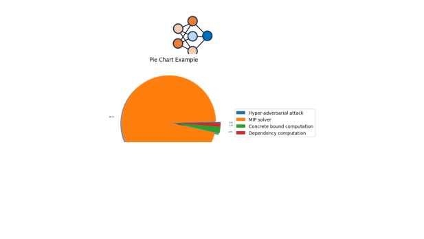
Figure 3. An example of the perturbation dependencies of an occlusion perturbation blackening the pixel $(1,1)$.

Consider Figure 3, showing an example of a small network comprising 16 inputs $z_{0,i,j}\in[0,1]$, two outputs $o_{1},o_{2}$, and two hidden layers. The first hidden layer is a convolutional layer composed from four ReLU neurons. The second hidden layer is a fully-connected layer composed from two ReLU neurons; its weights are depicted by the edges and its biases by the neurons. Consider the occlusion perturbation, blackening the pixel (1,1). Blackening it means setting its value to zero (i.e., the minimal pixel value). The figure shows, at the top, the input network, receiving the input, and, at the bottom, the perturbation network, receiving the perturbed example. By the encoding of Tjeng et al. (2019), each neuron of the input network has a real-valued variable, denoted $z_{m,i,j}$ for $m\in\{0,1\}$ (for the input layer and the convolutional layer), or $z_{m,k}$ for $m=2$ (for the fully-connected layer), where $i$, $j$, and $k$ are the indices within the layers. Each non-input neuron also has a boolean variable, denoted $a_{1,i,j}$ or $a_{2,k}$. Similarly, each neuron of the perturbation network has a real-valued variable, denoted $z^{p}_{m,i,j}$ for $m\in\{0,1\}$ and $z^{p}_{2,k}$, and each non-input neuron has a boolean variable, denoted $a^{p}_{1,i,j}$ or $a^{p}_{2,k}$. Because the occlusion perturbation changes a single input pixel, all input neurons besides $(1,1)$ are the same: $z_{0,i,j}=z^{p}_{0,i,j}$, for $(i,j)\in[4]\times[4]\setminus\{(1,1)\}$. Consequently, the computations of the subsequent layers are also related. In the convolutional layer, the neurons at indices $(1,2),(2,1),(2,2)$ accept the same values in the input and the perturbed networks, and the neuron at index (1,1) accepts smaller or equal values in the perturbed network compared to the input network (recall $z^{p}_{0,1,1}=0\leq z_{0,1,1}$). Thus, VHAGaR adds the dependencies: $z_{1,i,j}=z^{p}_{1,i,j}$ and $a_{1,i,j}=a^{p}_{1,i,j}$ for $(i,j)\in\{(1,2),(2,1),(2,2)\}$ as well as $z_{1,1,1}\geq z^{p}_{1,1,1}$ and $a_{1,1,1}\geq a^{p}_{1,1,1}$. Similarly, in the fully-connected layer, VHAGaR adds the dependencies $z_{2,1}\geq z^{p}_{2,1}$ and $a_{2,1}\geq a^{p}_{2,1}$, for the first neuron, and $z_{2,2}\leq z^{p}_{2,2}$ and $a_{2,2}\leq a^{p}_{2,2}$, for the second neuron. Adding these constraints to the MIP encoding prunes the search space. Further, it effectively removes three boolean variables.

4.3. Computing a Suboptimal Lower Bound by a Hyper-Adversarial Attack

In this section, we present our approach to expedite the tightening of the lower bound by efficiently computing a suboptimal feasible solution to Problem 2 and providing it to the MIP solver. Computing feasible solutions amounts to computing adversarial examples. This is because feasible solutions are inputs $x$ that have a perturbation amount $\mathcal{E}^{\prime}$ that leads the network to change its classification. We present a hyper-adversarial attack, generalizing existing adversarial attacks to unknown inputs. A hyper-adversarial attack leverages numerical optimization, which is more effective for finding adversarial examples, and thereby it expedites the lower bound computation of the general-purpose MIP solver. We also use the hyper-adversarial attack to provide the MIP solver hints (a partial assignment) for the optimization variables to further guide the MIP solver to the optimal solution.

An adversarial attack gets an input and computes a perturbation that misleads the network. In our global robustness setting, there is no particular input to attack. Instead, the space of feasible solutions (i.e., inputs) is defined by the constraint: $\exists x\exists\mathcal{E}^{\prime}\in I_{\mathcal{E}}.\ \mathcal{C}(x,c^{\prime},D)>\delta\wedge\mathcal{C}(f_{P}(x,\mathcal{E}^{\prime}),c^{\prime},D)\leq 0$. A hyper-adversarial attack begins by generating a hyper-input. A hyper-input is a set of $M$ inputs $X=\{x_{1},x_{2},x_{3},...,x_{M}\}$ classified as $c^{\prime}$. It consists of inputs with a wide range of class confidences. This property enables the hyper-adversarial attack to quickly converge to a non-trivial suboptimal (or optimal) lower bound. This is because the large variance in the confidences means some inputs are closer to the optimal lower bound. These inputs provide the optimizer with a good starting point to begin searching for the optimal value without knowing the optimal value. We demonstrate this property in Figure 4(b). Given a hyper-input $X$, a hyper-adversarial attack simultaneously looks for inputs that have adversarial examples with a higher class confidence than those of the inputs in $X$. Unlike existing adversarial attacks, a hyper-adversarial attack does not look for a perturbation that causes misclassification but rather for inputs that have perturbations that cause misclassification. Formally, given a hyper-input $X$, the hyper-adversarial attack is defined over input variables $\tilde{X}=(\tilde{x}_{1},\ldots,\tilde{x}_{M})^{T}$ and perturbation variables $\tilde{\mathcal{E}}^{\prime}=(\tilde{\mathcal{E}}^{\prime}_{1},\ldots,\tilde{\mathcal{E}}^{\prime}_{M})^{T}$, each corresponding to an input in $X$. The goal of the search is to find a vector $\tilde{X}$ that when added to the vector $X$ leads to at least one input with a higher class confidence that has an adversarial example. The corresponding optimization problem is the following multi-objective optimization problem:

(3) $$\begin{gathered}\max_{\tilde{X}}\mathcal{C}(x_{1}+\tilde{x}_{1},c^{\prime},D),...,\mathcal{C}(x_{M}+\tilde{x}_{M},c^{\prime},D)\;\hskip 3.41418pt\text{subject to}\bigvee_{x_{i}\in X}\ \exists\tilde{\mathcal{E}}^{\prime}_{i}.\ \mathcal{C}(f_{P}(x_{i}+\tilde{x}_{i},\tilde{\mathcal{E}}^{\prime}_{i}),c^{\prime},D)\leq 0\end{gathered}$$

Since all inputs in $X$ have a positive class confidence for $c^{\prime}$, we can replace the $M$ maximization objectives with a single equivalent objective defined as the sum over the $M$ individual objectives. By aggregating the objectives with a sum, we streamline the optimization process. To make this objective problem amenable to standard optimization approaches, we strengthen the constraint and replace the disjunction by a conjunction. To solve the constrained optimization, we employ a standard relaxation (e.g., (Carlini and Wagner., 2017; Chen et al., 2017; Tu et al., 2019; Szegedy et al., 2014)) and transform it into an unconstrained optimization by presenting $M$ optimization values $\lambda=\{\lambda_{1},\ldots,\lambda_{M}\}$ and adding the conjuncts as additional terms to the optimization goal. Overall, VHAGaR optimizes the following loss function:

$$\max_{\tilde{X},\tilde{\mathcal{E}}^{\prime}}\sum_{i=1}^{M}{\mathcal{C}(x_{i}+\tilde{x}_{i},c^{\prime},D)}-\sum_{i=1}^{M}{\lambda_{i}\cdot\mathcal{C}(f_{P}(x_{i}+\tilde{x}_{i},\tilde{\mathcal{E}}^{\prime}_{i}),c^{\prime},D)}$$

VHAGaR maximizes this loss by adapting the PGD attack (Madry et al., 2018) to consider adaptive $\lambda_{i}$ (explained in Section 5.3). A solution to this optimization is an assignment to the variables, from which VHAGaR obtains a set of solutions denoted as $y=(y_{1},\ldots,y_{M})$, where $y_{i}=x_{i}+\tilde{x}_{i}$. VHAGaR looks for the input $y^{*}\in y$ maximizing the class confidence. It then provides its confidence to the MIP solver as a lower bound for our optimization problem (Problem 2). Additionally, it provides the MIP solver optimization hints. A hint is an assignment to an optimization variable from which the MIP solver proceeds its search. VHAGaR computes hints for the boolean variables (i.e., $a_{m,k},a^{p}_{m,k}$), which play a significant role in the problem’s complexity. It does so by first running the feasible solutions and their perturbed examples through the network to obtain their assignment of the optimization variables. Then, it defines a hint for every boolean that has the same value for the majority of the feasible solutions. We rely on the majority to avoid biasing the optimization to a single feasible solution’s values. Next, we provide an example of our hyper-adversarial attack.

Figure 4. An example of running the hyper-adversarial attack to obtain a suboptimal lower bound on the maximal globally non-robust bound for the occlusion perturbation blackening the pixel (1, 1).

Example

Figure 4(a) shows a small network, which has 16 inputs $z_{0,i,j}\in[0,1]$, two outputs $o_{1},o_{2}$ defining two classes $C=\{c_{1},c_{2}\}$, and two hidden layers. The weights are shown by the edges and the biases by the neurons. We consider an occlusion perturbation that blackens the pixel (1,1). For simplicity’s sake, we consider a constant perturbation, which allows us to omit the perturbation variables $\tilde{\mathcal{E}}^{\prime}$. In this example, the hyper-adversarial attack looks for inputs maximizing the class confidence of $c^{\prime}=c_{1}$, whose perturbed examples are misclassified as $c_{2}$. VHAGaR begins from a hyper-input consisting of six inputs $X=(x_{1},\ldots,x_{6})$ classified as $c_{1}$ with the confidences $\{1,\dots,6\}$, respectively (Figure 4(a), left). Note that these inputs’ confidences are uniformly distributed over the range of confidences $[1,6]$, providing a wide range of confidences. VHAGaR then initializes for every input a respective variable $\widetilde{X}=(\tilde{x}_{1},\ldots,\tilde{x}_{6})$. Initially, $\tilde{x}_{i}=0$, for every $i$. VHAGaR then runs the PGD attack over the loss: $\max_{\tilde{X}}\sum_{i=1}^{6}{\mathcal{C}(x_{i}+\tilde{x}_{i},c^{\prime},D)}-\sum_{i=1}^{6}{\lambda_{i}\mathcal{C}(f_{P}(x_{i}+\tilde{x}_{i},\mathcal{E}^{\prime}),c^{\prime},D)}$, where $f_{P}$ and $\mathcal{E}^{\prime}$ capture blackening the pixel $(1,1)$. At a high-level, this attack runs iterations. An iteration begins by running each input $x_{i}+\tilde{x}_{i}$ through the network to compute $\mathcal{C}(x_{i}+\tilde{x}_{i},c^{\prime},D)$, and each $f_{P}(x_{i}+\tilde{x}_{i},\mathcal{E}^{\prime})$, which is identical to $x_{i}+\tilde{x}_{i}$ except for the black pixel, through the network to compute $\mathcal{C}(f_{P}(x_{i}+\tilde{x}_{i},\mathcal{E}^{\prime}),c^{\prime},D)$. Then, VHAGaR computes the gradient of the loss, updates $\widetilde{X}$ based on the gradient direction, and begins a new iteration, until it converges. On the right, the figure shows the inputs at the end of the optimization. In this example, all the respective perturbed examples are classified as $c_{2}$ and the maximal class confidence of $c_{1}$ is $2$. The value $2$ is submitted to the MIP solver as a lower bound on the maximal globally non-robust bound. This lower bound prunes for the MIP solver many exploration paths leading to inputs with class confidence lower than 2. For example, it prunes every exploration path in which $a_{1,i,j}=0$, for every $i$ and $j$. Thereby, it prunes every assignment in the following space: $\forall i\forall j.\ a_{1,i,j}=0\land\forall i.\ a_{2,i}\in\{0,1\}\land\forall i\forall j.\ a^{p}_{1,i,j}\in\{0,1\}\land\forall i.\ a^{p}_{2,i}\in\{0,1\}$. This pruning is obtained by bound propagation, a common technique in modern solvers. In addition to the lower bound, VHAGaR computes optimization hints by looking for boolean variables with the same assignment, for the majority of inputs or their perturbed examples. In this example, the hints are $\forall i\forall j.\ a_{1,i,j}=a^{p}_{1,i,j}=1$ and $\forall i.\ a_{2,i}=a_{2,i}^{p}=1$. These hints are identical to the boolean values corresponding to the optimal solution of Problem 2. By providing the hints to the MIP solver, it converges efficiently to a suboptimal (or optimal) solution.

Figure 4(b) shows how the class confidences $\mathcal{C}(x_{i}+\tilde{x}_{i},c_{1},D)$ (left) and $\mathcal{C}(f_{P}(x_{i}+\tilde{x}_{i},\mathcal{E}^{\prime}),c_{2},D)$ (right) change during the optimization, for all six inputs. The left plot shows that initially, since $\tilde{x}_{i}=0$, the confidences of $x_{i}+\tilde{x}_{i}$ are uniformly distributed. As the optimization progresses, the $\tilde{x}_{i}$-s are updated and eventually all $x_{i}+\tilde{x}_{i}$ converge to the optimal maximal globally non-robust bound, which is $2$. Note that inputs that initially have close confidences to the maximal globally non-robust bound converge faster than inputs that initially have a confidence that is farther from the bound. This demonstrates the importance of running the hyper-adversarial attack over inputs with a wide range of confidences: it enables to expedite the search for a feasible solution with a high confidence (we remind that the optimal bound is unknown to the optimizer and it may terminate before converging to all inputs). In particular, it increases the likelihood of reaching a suboptimal lower bound. The right plot shows how all perturbed examples are eventually classified as $c_{2}$.

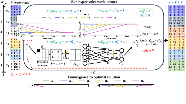
Figure 5. Illustration of VHAGaR.

5. VHAGaR: a Verifier of Hazardous Attacks for Global Robustness

In this section, we describe VHAGaR, our anytime system for computing an interval bounding the minimal globally robust bound (Definition 3.3). Figure 5 illustrates its operation. VHAGaR takes as arguments a classifier $D$, a class $c^{\prime}$, a set of target classes $C_{t}\subseteq C\setminus\{c^{\prime}\}$, a perturbation function $f_{P}$, and a perturbation range $I_{\mathcal{E}}$. Note that VHAGaR takes as input a set of target classes, thereby it can support the untargeted definition (where $C_{t}=C\setminus\{c^{\prime}\}$), the (single) targeted definition (where $C_{t}=\{c_{t}\}$ for some $c_{t}\neq c^{\prime}$), or any definition in between (where $C_{t}$ contains several classes). VHAGaR begins by encoding Problem 2 as a MIP. This encoding consists of two copies of the network computation, $\mathcal{D}$ for the input $x$ and $\mathcal{D}^{p}$ for the perturbed example $x^{p}$. To scale the MIP solver’s computation, VHAGaR computes concrete lower and upper bounds by adapting the approach of Tjeng et al. (2019). VHAGaR then adds a constraint $\phi_{in}$ capturing the dependencies stemming from the perturbation and a constraint $\phi_{dep}$ capturing dependencies over the two networks’ neurons. In parallel to the MIP encoding, VHAGaR computes for each class in $C_{t}$ a suboptimal lower bound $\delta^{HA}$ by running the hyper-adversarial attack. From the attack, it also obtains optimization hints and passes them to the MIP solver in two matrices, $\mathcal{H}$ for $\mathcal{D}$ and $\mathcal{H}^{p}$ for $\mathcal{D}^{p}$. We note that in our implementation, the MIP encoding is run on CPUs, and in parallel the hyper-adversarial attack runs on GPUs. After the MIP encoding and the hyper-adversarial attack complete, VHAGaR submits for every target class in $C_{t}$ a MIP to the MIP solver (in parallel). The solver returns the lower and upper bound for each MIP, computed given a timeout. The maximum lower and upper bounds over these bounds form the interval of the maximal globally non-robust bound. VHAGaR adds the precision level $\Delta$ and returns this interval, bounding the minimal globally robust bound. We next present the MIP encoding (Section 5.1), the dependency computation (Section 5.2), and the hyper-adversarial attack (Section 5.3). Finally, we discuss correctness and running time (Section 5.4).

5.1. The MIP Encoding

In this section, we present VHAGaR’s MIP encoding which adapts the encoding of Tjeng et al. (2019) for local robustness verification. To understand VHAGaR’s encoding, we first provide background on encoding local robustness as a MIP, for a fully-connected classifier (the extension to a convolutional network is similar). Then, we describe our adaptations for our global robustness setting.

Background

Tjeng et al. (2019) propose a sound and complete local robustness analysis by encoding this task as a MIP problem. A classifier $D$ is locally robust at a neighborhood of an input $x$ if all inputs in the neighborhood are classified as some class $c^{\prime}$. Tjeng et al. (2019)’s verifier gets as arguments a classifier $D$, an input $x$ classified as $c^{\prime}$, and a neighborhood $\mathcal{N}(x)$ defined by a series of intervals bounding each input entry, i.e., $x^{\prime}\in\mathcal{N}(x)$ if and only if $x^{\prime}_{k}\in[l_{k},u_{k}]$, where $k$ is the $k^{\text{th}}$ input entry. The verifier generates a MIP for every target class $c_{t}\neq c^{\prime}$. If there is no solution to the MIP of $c_{t}$, all inputs in $\mathcal{N}(x)$ are not classified as $c_{t}$; otherwise, there is an input classified as $c_{t}$. If no MIP has a solution, the network is locally robust at $\mathcal{N}(x)$. The verifier encodes the local robustness analysis as follows. It introduces a real-valued variable for every input neuron, denoted $z_{0,k}$. The input neurons are subjected to the neighborhood’s bounds: $\forall k.\ l_{k}\leq z_{0,k}\leq u_{k}$. Each internal neuron has two real-valued variables $\hat{z}_{m,k}$, for the affine computation, and ${z}_{m,k}$, for the ReLU computation. The affine computation is straightforward: $\hat{z}_{m,k}=b_{m,k}+\sum_{k^{\prime}=1}^{k_{m-1}}{w}_{m,k,k^{\prime}}\cdot{z}_{m-1,k^{\prime}}$. For the ReLU computation, the verifier introduces a boolean variable $a_{m,k}$ and two concrete lower and upper bounds $l_{m,k},u_{m,k}\in\mathbb{R}$, bounding the possible values of the input $\hat{z}_{m,k}$. The verifier encodes ReLU by the constraints: ${z}_{m,k}\geq 0$, ${z}_{m,k}\geq\hat{z}_{m,k}$, ${z}_{m,k}\leq u_{m,k}\cdot a_{m,k}$, and ${z}_{m,k}\leq\hat{z}_{m,k}-l_{m,k}(1-a_{m,k})$. The concrete bounds are computed by solving the optimization problems $l_{m,k}=\min z_{m,k}$ and $u_{m,k}=\max z_{m,k}$ where the constraints are the encodings of all previous layers. We denote the set of constraints pertaining to the neurons by $\mathcal{D}$. To determine local robustness, the verifier duplicates the above constraints $|C|-1$ times, once for every class $c_{t}\neq c^{\prime}$. For every $c_{t}$, the verifier adds the constraint $z_{L,c_{t}}-z_{L,c^{\prime}}>0$ where $L$ is the output layer. This constraint checks whether there is an input in the neighborhood whose $c_{t}$’s score is higher than $c^{\prime}$’s score. If the constraints of the MIP of $c_{t}$ are satisfied, the neighborhood has an input not classified as $c^{\prime}$ and hence it is not locally robust. Otherwise, no input in the neighborhood is classified as $c_{t}$. Overall, if at least one of the $|C|-1$ MIPs is satisfied, the neighborhood is not locally robust; otherwise, it is locally robust.

Adaptations

VHAGaR builds on the above encoding to compute the maximal globally non-robust bound. We next describe our adaptations supporting (1) analysis of global robustness over any input and its perturbed example, (2) encoding dependencies between the MIP variables, and (3) encoding the globally non-robust bound $\delta_{c^{\prime},c_{t}}$ and its lower bound $\delta^{HA}_{c^{\prime},c_{t}}$.

To support global robustness analysis, VHAGaR has to consider any input and its perturbed example. Thus, VHAGaR has two copies of the above variables and constraints. The first copy is used for the input, while the second copy is used for the perturbed example, and its variables are denoted with a superscript $p$. We denote the set of constraints of the network propagating the perturbed example by $\mathcal{D}^{p}$. To capture $x^{p}=f_{P}(x,\mathcal{E^{\prime}})$, VHAGaR adds an input constraint $\phi_{in}$ (defined in Section 5.2.2). VHAGaR encodes $\mathcal{E^{\prime}}\in I_{\mathcal{E}}$, limiting the amount of perturbation, by a constraint bounding each entry of $\mathcal{E}^{\prime}$ in its interval in $I_{\mathcal{E}}$. Additionally, VHAGaR computes dependencies between the MIP variables. These dependencies emerge from the input dependencies, the perturbation range $I_{\mathcal{E}}$, and the network’s computation. The dependencies enable VHAGaR to reduce the problem’s complexity without affecting the soundness and completeness of the encoding. The dependency constraint $\phi_{dep}$ involves running additional MIPs (described in Section 5.2).

To encode the maximization of the globally non-robust bound $\delta$, VHAGaR performs the following adaptations. First, for every target class $c_{t}$, it introduces a variable $\delta_{c^{\prime},c_{t}}$ capturing the maximal globally non-robust bound targeting $c_{t}$. Namely, it is the maximal class confidence of $c^{\prime}$ of an input for which there exists a perturbed example that is misclassified as $c_{t}$. Accordingly, it adds as an objective: $\max\delta_{c^{\prime},c_{t}}$. Note that by adding this objective, VHAGaR can solve the MIP in an anytime manner, because it looks for a number (the bound) and not a yes/no answer (like local robustness). Second, it replaces the last constraint of the input’s network $z_{L,c_{t}}-z_{L,c^{\prime}}>0$ by constraints requiring that the class confidence of $c^{\prime}$ is higher than $\delta_{c^{\prime},c_{t}}$: $\forall c^{\prime\prime}\in C\setminus\{c^{\prime}\}.\ z_{L,c^{\prime}}-z_{L,c^{\prime\prime}}>\delta_{c^{\prime},c_{t}}$. Third, the constraint $\mathcal{C}(f_{P}(x,\mathcal{E^{\prime}}),c_{t},D)>0$ is captured by the input constraint $\phi_{in}$ and the constraints (replacing the last constraint): $\forall c^{\prime\prime}\in C\setminus\{c_{t}\}.\ z^{p}_{L,c_{t}}-z^{p}_{L,c^{\prime\prime}}>0$. Lastly, it adds the constraint $\delta_{c^{\prime},c_{t}}\geq\delta_{c^{\prime},c_{t}}^{HA}$, where $\delta_{c^{\prime},c_{t}}^{HA}$ is the lower bound computed by the hyper-adversarial attack. To conclude, VHAGaR submits to the solver the following maximization problem for each $c_{t}$:

(4) $$\begin{gathered}\max\delta_{c^{\prime},c_{t}}\hskip 14.22636pt\text{subject to}\\ \mathcal{E^{\prime}}\in I_{\mathcal{E}};\hskip 7.68236pt\phi_{in};\hskip 7.68236pt\phi_{dep};\hskip 7.68236pt\delta_{c^{\prime},c_{t}}\geq\delta^{HA}_{c^{\prime},c_{t}};\hskip 7.68236pt\forall{c^{\prime\prime}\neq c^{\prime}}.\ z_{L,c^{\prime}}-z_{L,c^{\prime\prime}}>\delta_{c^{\prime},c_{t}};\hskip 7.68236pt\forall c^{\prime\prime}\neq c_{t}.\ z^{p}_{L,c_{t}}-z^{p}_{L,c^{\prime\prime}}>0\\ \forall m\forall k:\hskip 14.22636pt\;\hat{z}_{m,k}=b_{m,k}+\sum_{k^{\prime}=1}^{k_{m-1}}{w}_{m,k,k^{\prime}}\cdot{z}_{m-1,k^{\prime}};\hskip 14.22636pt\hat{z}^{p}_{m,k}=b_{m,k}+\sum_{k^{\prime}=1}^{k_{m-1}}{w}_{m,k,k^{\prime}}\cdot{z^{p}}_{m-1,k^{\prime}}\\ {z}_{m,k}\geq 0;\hskip 14.22636pt{z}_{m,k}\geq\hat{z}_{m,k};\hskip 14.22636pt{z}_{m,k}\leq u_{m,k}\cdot a_{m,k};\hskip 14.22636pt\;{z}_{m,k}\leq\hat{z}_{m,k}-l_{m,k}(1-a_{m,k})\\ {z^{p}}_{m,k}\geq 0;\hskip 14.22636pt{z^{p}}_{m,k}\geq\hat{z}^{p}_{m,k};\hskip 14.22636pt{z^{p}}_{m,k}\leq u^{p}_{m,k}\cdot a^{p}_{m,k};\hskip 14.22636pt{z^{p}}_{m,k}\leq\hat{z}^{p}_{m,k}-l^{p}_{m,k}(1-a^{p}_{m,k})\\ \end{gathered}$$

From the above encoding, we get the next two lemmas.

Lemma 5.1.

An optimal solution to the above MIP $\delta^{*}_{c^{\prime},c_{t}}$ is the maximal globally non-robust bound targeting $c_{t}$. Consequently, $\delta^{*}=\max_{c_{t}\neq c^{\prime}}\delta^{*}_{c^{\prime},c_{t}}$ is the maximal globally non-robust bound.

Lemma 5.2.

The minimal globally robust bound is $\delta=\delta^{*}+\Delta$, where $\Delta>0$ is the precision level.

5.2. Leveraging Dependencies to Reduce the Complexity

In this section, we explain how to identify dependencies between the MIP’s variables that enable to reduce the complexity of the MIP problem. VHAGaR incorporates the dependencies via the constraints $\phi_{in}$, for dependencies between the input and its perturbed example, and $\phi_{dep}$ for dependencies between neurons of the two network copies. Input dependencies are defined by the perturbation. Neuron dependencies are computed by VHAGaR from the neurons’ concrete bounds, dependency propagation from preceding layers, or MIPs. We focus on input constraints $\phi_{in}$ defined by linear or quadratic constraints and dependency constraints $\phi_{dep}$ defined by equalities or inequalities over the optimization variables, all are supported by standard MIP solvers.

5.2.1. Dependency Constraint

We begin with describing the dependency constraint $\phi_{dep}$. The goal is to identify pairs of neurons $z_{m,k}$ and $z^{p}_{m^{\prime},k^{\prime}}$, one from the input’s network and the other one from the perturbed example’s network, that satisfy equality or inequality constraint: $z_{m,k}\bowtie z^{p}_{m^{\prime},k^{\prime}}$, where $\bowtie\in\{\leq,<,\geq,>,=\}$. These constraints prune the search space. To determine whether $z_{m,k}\bowtie z^{p}_{m^{\prime},k^{\prime}}$, for $\bowtie\in\{\leq,<,\geq,>,=\}$, one can solve a maximization and a minimization problems, each is over the constraints of Problem 4 up to layers $m$ and $m^{\prime}$, $\phi_{in}$, and the current $\phi_{dep}$ where the objectives are:

$$\begin{multlined}\phantom{aa}u_{m,k,m^{\prime},k^{\prime}}=\text{max }\>{z_{m,k}-z^{p}_{m^{\prime},k^{\prime}}}\;\;\;l_{m,k,m^{\prime},k^{\prime}}=\text{min}\>{z_{m,k}-z^{p}_{m^{\prime},k^{\prime}}}\end{multlined}\phantom{aa}u_{m,k,m^{\prime},k^{\prime}}=\text{max }\>{z_{m,k}-z^{p}_{m^{\prime},k^{\prime}}}\;\;\;l_{m,k,m^{\prime},k^{\prime}}=\text{min}\>{z_{m,k}-z^{p}_{m^{\prime},k^{\prime}}}$$

The values of $u_{m,k,m^{\prime},k^{\prime}}$ and $l_{m,k,m^{\prime},k^{\prime}}$ determine the relation between $z_{m,k}$ and $z^{p}_{m^{\prime},k^{\prime}}$ as follows:

Lemma 5.3.

Given two variables, $z_{m,k}$ and $z^{p}_{m^{\prime},k^{\prime}}$ and their boolean variables $a_{m,k}$ and $a^{p}_{m^{\prime},k^{\prime}}$:

• if $u_{m,k,m^{\prime},k^{\prime}}=l_{m,k,m^{\prime},k^{\prime}}=0$, then $z_{m,k}=z^{p}_{m^{\prime},k^{\prime}}$ and $a_{m,k}=a^{p}_{m^{\prime},k^{\prime}}$.

• if $l_{m,k,m^{\prime},k^{\prime}}\bowtie 0$, then $z_{m,k}\bowtie z^{p}_{m^{\prime},k^{\prime}}$ and $a_{m,k}\geq a^{p}_{m^{\prime},k^{\prime}}$, where $\bowtie\in\{\geq,>\}$.

• if $u_{m,k,m^{\prime},k^{\prime}}\bowtie 0$, then $z_{m,k}\bowtie z^{p}_{m^{\prime},k^{\prime}}$ and $a_{m,k}\leq a^{p}_{m^{\prime},k^{\prime}}$, where $\bowtie\in\{\leq,<\}$.

The proof follows from the MIPs and the monotonicity of ReLU. Solving these maximization and minimization problems for all combinations of $(m,k)$ and $(m^{\prime},k^{\prime})$ would significantly increase the complexity of VHAGaR and is thus impractical. To cope, VHAGaR focuses on two kinds of dependencies: those stemming directly from the perturbation and those stemming from the computation of corresponding neurons (i.e., $m^{\prime}=m$ and $k^{\prime}=k$). For the first kind of dependencies, VHAGaR adds the input dependencies (Section 5.2.2) and employs dependency propagation (defined shortly), neither requires solving the above optimization problems. For the second kind of dependencies, VHAGaR first checks the concrete bounds: if the lower bound of $z_{m,k}$ is greater than the upper bound of $z_{m,k}^{p}$, then $z_{m,k}>z^{p}_{m,k}$ and vice-versa. Otherwise, VHAGaR computes the dependencies by solving the minimization and maximization problems (only for corresponding neuron pairs).

We next define dependency propagation. A dependency is propagated for a pair of neurons in the same layer $z_{m,k}$ and $z^{p}_{m,k^{\prime}}$ if their inputs share dependencies that are preserved or reversed for $z_{m,k}$ and $z^{p}_{m,k^{\prime}}$ because of their linear transformations and the ReLU definition:

Lemma 5.4 (Dependency Propagation).

Given a neuron $z_{m,k}$ and a neuron $z^{p}_{m,k^{\prime}}$ then:

• if  $\forall i\ (w_{m,k,k_{i}}\cdot z_{m-1,k_{i}}=w_{m,k^{\prime},k^{\prime}_{i}}\cdot z^{p}_{m-1,k^{\prime}_{i}})$, then $z_{m,k}=z^{p}_{m,k^{\prime}}$ and $a_{m,k}=a^{p}_{m,k^{\prime}}$.

• if  $\forall i\ (w_{m,k,k_{i}}\cdot z_{m-1,k_{i}}\geq w_{m,k^{\prime},k^{\prime}_{i}}\cdot z^{p}_{m-1,k^{\prime}_{i}})$, then ${z}_{m,k}\geq{z}^{p}_{m,k^{\prime}}$ and ${a}_{m,k}\geq{a}^{p}_{m,k^{\prime}}$.

• if  $\forall i\ (w_{m,k,k_{i}}\cdot z_{m-1,k_{i}}\leq w_{m,k^{\prime},k^{\prime}_{i}}\cdot z^{p}_{m-1,k^{\prime}_{i}})$, then ${z}_{m,k}\leq{z}^{p}_{m,k^{\prime}}$ and ${a}_{m,k}\leq{a}^{p}_{m,k^{\prime}}$.

VHAGaR generally uses the lemma for $k^{\prime}=k$, except for geometric perturbations (translation and rotation). In this case, it uses the lemma for indices whose correspondence stems from the perturbation, e.g., $k^{\prime}=k+1$ for a translation perturbation that moves the pixels by one coordinate.

Example

We next exemplify how VHAGaR uses this lemma. Consider the small network and the occlusion perturbation blackening the pixel $(1,1)$, presented in Figure 3. VHAGaR sets the dependencies in a matrix, called $\phi_{dep}$. An entry $(m,k)$ corresponds to the dependency constraint of the neuron $z_{m,k}$, where the entries at $(0,k)$ store the dependencies of the input neurons. Additionally, it transforms index pairs $(i,j)\in[d_{1}]\times[d_{2}]$ to a single index: $k=(i-1)\cdot d_{2}+j\in[d_{1}\cdot d_{2}]$. Because the occlusion perturbation is not geometric, we focus on the dependencies of respective neurons $k=k^{\prime}$. In this case, the weights are equal and Lemma 5.4 is simplified to the following cases:

• if  $\forall i.\ w_{m,k,k_{i}}\cdot(z_{m-1,k_{i}}-z^{p}_{m-1,k_{i}})=0$, then $z_{m,k}=z^{p}_{m,k}$ and $a_{m,k}=a^{p}_{m,k}$.

• if  $\forall i.\ w_{m,k,k_{i}}\cdot(z_{m-1,k_{i}}-z^{p}_{m-1,k_{i}})\geq 0$, then ${z}_{m,k}\geq{z}^{p}_{m,k}$ and ${a}_{m,k}\geq{a}^{p}_{m,k}$.

• if  $\forall i.\ w_{m,k,k_{i}}\cdot(z_{m-1,k_{i}}-z^{p}_{m-1,k_{i}})\leq 0$, then ${z}_{m,k}\leq{z}^{p}_{m,k}$ and ${a}_{m,k}\leq{a}^{p}_{m,k}$.

VHAGaR first encodes the dependencies stemming from the occlusion perturbation (defined in Section 5.2.2):

• $\phi_{dep}[0,1]=\{z_{0,1}\geq z^{p}_{0,1}\}$, since $z^{p}_{0,1}=0$ and $z_{0,1}\in[0,1]$, and

• $\forall k\in[2,16].\ \phi_{dep}[0,k]=\{z_{0,k}=z^{p}_{0,k}\}$, since the perturbation does not change these pixels.

These dependencies are propagated to the first layer as follows:

• $\phi_{dep}[1,1]=\{z_{1,1}\geq z_{1,1}^{p}\}$. This constraint, corresponding to the neuron $z_{1,1}$, follows from the second bullet of Lemma 5.4. To check that the second bullet holds, VHAGaR inspects the dependency constraints of the inputs to $z_{1,1}$ which are $z_{0,1},z_{0,2},z_{0,5},z_{0,6}$. It observes the following constraints: $\phi_{dep}[0,1]=\{z_{0,1}\geq z^{p}_{0,1}\}$ and the weight $w_{1,1,1}=1\geq 0$, and $\phi_{dep}[0,k]=\ \{z_{1,k}=z_{1,k}^{p}\}$, for $k\in\{2,5,6\}$. Since the precondition of the second bullet holds, VHAGaR adds the dependency constraint.

• $\phi_{dep}[1,k]=\{z_{1,k}=z_{1,k}^{p}\}$, for $k\in\{2,3,4\}$. These constraints, corresponding to the neurons $z_{1,2}$, $z_{1,3}$, and $z_{1,4}$, follow from the first bullet of Lemma 5.4. To check that the first bullet holds, VHAGaR inspects the dependency constraints of the inputs to each of these neurons and observes that all have an equality constraint. Since the precondition of the first bullet holds, VHAGaR adds the constraints.

These dependencies are propagated to the second layer as follows:

• $\phi_{dep}[2,1]=\{z_{2,1}\geq z_{2,1}^{p}\}$. This constraint, corresponding to the neuron $z_{2,1}$, follows from the second bullet of Lemma 5.4, since $\phi_{dep}[1,1]=\{z_{1,1}\geq z^{p}_{1,1}\}$, the weight $w_{2,1,1}=1$ is positive, and the dependencies of the other inputs are $\phi_{dep}[1,k]=\{z_{1,k}=z^{p}_{1,k}\}$, for $k>1$.

• $\phi_{dep}[2,2]=\{z_{2,2}\leq z^{p}_{2,2}\}$. This constraint, corresponding to the neuron $z_{2,2}$, follows from the third bullet of Lemma 5.4, since $\phi_{dep}[1,1]=\{z_{1,1}\geq z^{p}_{1,1}\}$, the weight $w_{2,1,2}=-1$ is negative, and the dependencies of the other inputs are equalities.

Input: A perturbation $f_{P}$, its range $I_{\mathcal{E}}$, an input constraint $\phi_{in}$, the network encodings $\mathcal{D}$, $\mathcal{D}^{p}$.

Output: A dependency constraint $\phi_{dep}$.

1

2$\phi_{dep}[L+1,\max\{k_{1},\ldots,k_{L}\}]=\bot$

3 $\phi_{dep}$ = add_perturbation_dep($f_{P},I_{\mathcal{E}}$, $\phi_{in}$, $\mathcal{D}$, $\mathcal{D}^{p}$, $\phi_{dep}$)

4 foreach layer$\;m\in\{1,\dots,L\}$ do

5       foreach neuron$\;k\in\{1,\dots,k_{m}\}$ do

6             if $\phi_{dep}[m,k]\neq\bot$ then  continue

7             if $l_{m,k}>u^{p}_{m,k}$ then  $\phi_{dep}[m,k]=\{z_{m,k}>z^{p}_{m,k},a_{m,k}\geq a^{p}_{m,k}\}$

8             else if $u_{m,k}<l^{p}_{m,k}$ then  $\phi_{dep}[m,k]=\{z_{m,k}<z^{p}_{m,k},a_{m,k}\leq a^{p}_{m,k}\}$

9             else

10                   $\phi_{dep}[m,k]$ = dependencies_propagation($m$, $k$, $\mathcal{D}$, $\mathcal{D}^{p}$, $\phi_{dep}$)

11                   if $\phi_{dep}[m,k]\neq\bot$ then  continue

12                   $u_{m,k,m,k}=\infty$ , $l_{m,k,m,k}=-\infty$

13                   if $[l_{m,k},u_{m,k}]\sqcap[l^{p}_{m,k},u^{p}_{m,k}]==[l_{m,k},u^{p}_{m,k}]$ then

14                        

15                        $l_{m,k,m,k}=\mathbb{min_{\text{cutoff}=0}}\>\>z_{m,k}-z^{p}_{m,k}\>s.t.\>\mathcal{E^{\prime}}\in I_{\mathcal{E}},\phi_{in},\phi_{dep},\mathcal{D}_{1:m},\mathcal{D}^{p}_{1:m}$

16                  if $[l_{m,k},u_{m,k}]\sqcap[l^{p}_{m,k},u^{p}_{m,k}]==[l^{p}_{m,k},u_{m,k}]$ then

17                        

18                        $u_{m,k,m,k}=\mathbb{max_{\text{cutoff}=0}}\>\>z_{m,k}-z^{p}_{m,k}\>s.t.\>\mathcal{E^{\prime}}\in I_{\mathcal{E}},\phi_{in},\phi_{dep},\mathcal{D}_{1:m},\mathcal{D}^{p}_{1:m}$

19                  

20                  if ($[l_{m,k,m,k},u_{m,k,m,k}]==[0,0]$) then  $\phi_{dep}[m,k]=\{z_{m,k}=z^{p}_{m,k},a_{m,k}=a^{p}_{m,k}\}$

21                   else if $l_{m,k,m,k}\geq 0$ then  $\phi_{dep}[m,k]=\{z_{m,k}\geq z^{p}_{m,k},a_{m,k}\geq a^{p}_{m,k}\}$

22                   else if $u_{m,k,m,k}\leq 0$ then  $\phi_{dep}[m,k]=\{z_{m,k}\leq z^{p}_{m,k},a_{m,k}\leq a^{p}_{m,k}\}$

23                  

24            

25      if  $\forall k.\>\phi_{dep}[m,k]==\bot$ then break

26      

return $\bigwedge\{\phi_{dep}[m,k]\>|\>\phi_{dep}[m,k]\neq\bot,m>0\}$

Algorithm 1 Compute_dependency_constraints($f_{P}$, $I_{\mathcal{E}}$, $\phi_{in}$, $\mathcal{D}$, $\mathcal{D}^{p}$)

Algorithm

Algorithm 1 shows how VHAGaR computes the dependencies. Its inputs are the perturbation function $f_{P}$, its range $I_{\mathcal{E}}$, the input constraint $\phi_{in}$, and the classifier encodings $\mathcal{D}$ and $\mathcal{D}^{p}$. It begins by initializing a matrix, whose rows are the layers (including the input layer) and its columns are the neurons in each layer. An entry $(m,k)$ in the matrix corresponds to the dependency constraint of the neuron $z_{m,k}$ (Algorithm 1). VHAGaR begins by adding the perturbation’s dependencies for the relevant neurons, as defined in Section 5.2.2 (Algorithm 1). VHAGaR then iterates over all neurons, layer-by-layer, and computes dependencies (Algorithm 1–Algorithm 1). If an entry $(m,k)$ is not empty, it is skipped (Algorithm 1). Otherwise, if $l_{m,k}$, the lower bound of $z_{m,k}$, is greater than $u_{m,k}^{p}$, the upper bound of $z^{p}_{m,k}$, then $z_{m,k}>z^{p}_{m,k}$ and vice-versa (Algorithm 1–Algorithm 1). Then, VHAGaR checks whether it can propagate a dependency (Algorithm 1). If not, VHAGaR checks whether it should solve the optimization problems. The minimization problem is solved if $l^{p}_{m,k}\leq l_{m,k}\leq u^{p}_{m,k}\leq u_{m,k}$, in which case it may be that $z_{m,k}\geq z^{p}_{m,k}$ (Algorithm 1–Algorithm 1). Similarly, the maximization problem is solved if $l_{m,k}\leq l^{p}_{m,k}\leq u_{m,k}\leq u^{p}_{m,k}$, in which case it may be that $z^{p}_{m,k}\geq z_{m,k}$ (Algorithm 1–Algorithm 1). Note that if $l^{p}_{m,k}<l_{m,k}\leq u_{m,k}<u^{p}_{m,k}$, the two variables are incomparable since $z^{p}_{m,k}$ may be equal to $l^{p}_{m,k}$ (and thus $z^{p}_{m,k}<z_{m,k}$) or equal to $u^{p}_{m,k}$ (and thus $z_{m,k}<z^{p}_{m,k}$). Similarly, the two variables are incomparable if $l_{m,k}<l^{p}_{m,k}\leq u^{p}_{m,k}<u_{m,k}$. The minimization problem early stops when the lower bound on the objective reaches zero or when the upper bound becomes negative. The maximization problem early stops when the upper bound on the objective reaches zero or when the lower bound becomes positive. This is because the optimal minimal and maximal values are not required to determine the relation between the variables. If both returned values are zero, the variables are equal. Otherwise, if the minimal value is at least zero, then $z_{m,k}\geq z^{p}_{m,k}$, and if the maximal value is at most zero, then $z_{m,k}\leq z^{p}_{m,k}$ (Algorithm 1–Algorithm 1). The boolean variables have a similar dependency. In case no pair of neurons depends in the current layer, the algorithm terminates (Algorithm 1). Finally, the algorithm returns all dependencies (Algorithm 1).

5.2.2. Input Dependencies

Lastly, we describe the input dependencies $\phi_{in}$ and define the dependencies’ encoding for several semantic perturbations and the $L_{\infty}$ perturbation. These perturbations have been shown to inflict adversarial examples (Goodfellow et al., 2015; Mohapatra et al., 2020; Engstrom et al., 2019, 2017; Goswami et al., 2018; Wu et al., 2019; Liu et al., 2019). Our definitions assume grayscale images, for simplicity’s sake, but VHAGaR supports colored images. To align with our MIP encoding, we transform index pairs $(i,j)\in[d_{1}]\times[d_{2}]$ to a single index: $k=(i-1)\cdot d_{2}+j\in[d_{1}\cdot d_{2}]$.

Brightness$([l,u])$

Brightness, whose range is an interval $-1\leq l\leq u\leq 1$, adds a value $\mathcal{E^{\prime}}\in[l,u]$ to the input $x$. Namely, $\phi_{in}=\forall k.\ (z^{p}_{0,k}=z_{0,k}+\mathcal{E^{\prime}})$. To enhance the encoding accuracy, VHAGaR adds constraints depending on the sign of $\mathcal{E^{\prime}}$. Given the sign of $\mathcal{E^{\prime}}$, VHAGaR computes the sign of the first layer $s=sign(\mathcal{E^{\prime}}\sum_{i^{\prime}}w_{1,k,i^{\prime}})$, and adds $\forall k.\ \phi_{dep}[1,k]=\{{z}_{1,k}\bowtie{z}^{p}_{1,k},{a}_{1,k}\bowtie{a}^{p}_{1,k}\}$, where $\bowtie\triangleq\leq$ if $s=+$, $\bowtie\triangleq\geq$ if $s=-$, and $\bowtie\triangleq=$ if $s=0$. The sign of $\mathcal{E^{\prime}}$ is $-$ if $u\leq 0$ and is $+$ if $l\geq 0$. Otherwise, VHAGaR duplicates the encoding and handles the cases $\mathcal{E^{\prime}}\in[l,0]$ and $\mathcal{E^{\prime}}\in[0,u]$ separately. VHAGaR propagates dependencies to subsequent layers as defined in Lemma 5.4.

Contrast$([l,u])$

Contrast, whose range is an interval $l\leq u\in\mathbb{R^{+}}$, multiplies the input by a value $\mathcal{E^{\prime}}\in[l,u]$. Namely, $\phi_{in}=\forall k.\ (z^{p}_{0,k}=\mathcal{E^{\prime}}\cdot z_{0,k})$. To propagate dependencies as in Lemma 5.4, VHAGaR also adds the constraints $\forall k.\ \phi_{dep}[0,k]=\{{z_{0,k}\bowtie z^{p}_{0,k}}\}$, where $\bowtie\triangleq\leq$ if $\mathcal{E^{\prime}}\geq 1$, and $\bowtie\triangleq\geq$ if $\mathcal{E^{\prime}}\leq 1$. The condition $\mathcal{E^{\prime}}\geq 1$ is true if $l\geq 1$; the condition $\mathcal{E^{\prime}}\leq 1$ is true if $u\leq 1$; otherwise, VHAGaR duplicates the encoding and handles the cases $\mathcal{E^{\prime}}\in[l,1]$ and $\mathcal{E^{\prime}}\in[1,u]$ separately.

Occlusion$([i_{l},i_{u}],[j_{l},j_{u}],[w_{l},w_{u}])$

Occlusion’s range is three intervals $1\leq i_{l}\leq i_{u}\leq d_{1}$; $1\leq j_{l}\leq j_{u}\leq d_{2}$ and $1\leq w_{l}\leq w_{u}\leq min(d_{1}-i_{u},d_{2}-j_{u})$. It perturbs based on a triple $(i,j,w)$, where $(i,j)$ defines the top-left coordinate of the occlusion square $S$ and $w$ is its length. The perturbation function maps every pixel in the square to zero; other pixels remain as are, namely $\phi_{in}=\forall k.\ (k\in S\Rightarrow z^{p}_{0,k}=0)\wedge(k\notin S\Rightarrow z^{p}_{0,k}=z_{0,k})$. To propagate dependencies as in Lemma 5.4, VHAGaR also adds the constraints $\forall k\in S.\ \phi_{dep}[0,k]=\{z_{0,k}\geq z^{p}_{0,k}\}$ and $\forall k\notin S.\ \phi_{dep}[0,k]=\{z_{0,k}=z^{p}_{0,k}\}$.

Patch$([0,\epsilon],[i_{l},i_{u}],[j_{l},j_{u}],[w_{l},w_{u}])$

Patch’s range consists of a perturbation limit $\epsilon\in(0,1]$ and the three intervals as defined in the occlusion’s range. A patch is defined by a top-left coordinate $(i,j)$ of the patch’s square $S$ and the patch length $w$. Its function, generalizing occlusion, perturbs every pixel in the patch by a value in the interval $[-\epsilon,\epsilon]$ (unlike occlusion which maps to zero); other pixels remain as are, namely: $\phi_{in}=\forall k.\ ({k\in S}\Rightarrow\ z^{p}_{0,k}\leq z_{0,k}+\epsilon\wedge z^{p}_{0,k}\geq z_{0,k}-\epsilon)\wedge(k\notin S\Rightarrow z^{p}_{0,k}=z_{0,k})$. Note that since every pixel in $S$ can be perturbed or keep its original value, a patch defined by $(i,j)$ and $w$ also contains every smaller, subsumed patch. To propagate dependencies as in Lemma 5.4, VHAGaR also adds the constraints $\forall k\notin S.\ \phi_{dep}[0,k]=\{z_{0,k}=z^{p}_{0,k}\}$.

Translation$([t_{x}^{l},t_{x}^{u}],[t_{y}^{l},t_{y}^{u}])$

Translation’s range is two intervals $-d_{1}\leq t_{x}^{l}\leq t_{x}^{u}\leq d_{1}$ and $-d_{2}\leq t_{y}^{l}\leq t_{y}^{u}\leq d_{2}$. Given a coordinate $(t_{x},t_{y})$, the perturbation function moves every pixel by $(t_{x},t_{y})$, namely $\phi_{in}=\forall(i,j).\ (i-t_{x}\notin[d_{1}]\lor j-t_{y}\notin[d_{2}]\Rightarrow z^{p}_{0,k}=0)\wedge(i-t_{x}\in[d_{1}]\wedge j-t_{y}\in[d_{2}]\Rightarrow z^{p}_{0,k}=z_{0,k-t_{x}\cdot d_{2}-t_{y}})$. To propagate dependencies as in Lemma 5.4, VHAGaR also adds a constraint for every $k=(i-1)\cdot d_{2}+j$: if $(i-t_{x}\notin[d_{1}]\lor j-t_{y}\notin[d_{2}])$ then $\phi_{dep}[0,k]=\{z_{0,k}\geq z^{p}_{0,k}\}$, otherwise $\phi_{dep}[0,k]=\{z_{0,k-t_{x}\cdot d_{2}-t_{y}}=z^{p}_{0,k}\}$.

Rotation$([\theta_{l},\theta_{u}])$

Rotation, whose range is an interval $0\leq\theta_{l}\leq\theta_{u}\leq 360$, rotates the input by an angle $\theta$ using a standard rotation algorithm. The algorithm (Appendix A) begins by centralizing the pixel coordinates, i.e., a coordinate $(i,j)$ is mapped to $i_{c}=i-d_{1}/2$ and $j_{c}=j-d_{2}/2$. The centralized coordinates are rotated by $i_{r}=i_{c}\cdot\sin(\frac{\theta\cdot\pi}{180})+j_{c}\cdot\cos(\frac{\theta\cdot\pi}{180}))+d_{1}/2$ and $j_{r}=(i_{c}\cdot\cos(\frac{\theta\cdot\pi}{180})-j_{c}\sin(\frac{\theta\cdot\pi}{180})+d_{2}/2$. Finally, a bilinear interpolation is executed. Namely, $\phi_{in}=\forall(i,j).\ (1\leq i_{r}\leq d_{1}\wedge\;1\leq j_{r}\leq d_{2}\Rightarrow\>z^{p}_{0,k}=\text{bilinear\_interpolation}(z_{0,k},i_{r},j_{r}))\wedge(i_{r}<1\lor i_{r}>d_{1}\lor j_{r}<1\lor j_{r}>d_{2}\Rightarrow z^{p}_{0,k}=0)$. To propagate dependencies as in Lemma 5.4, VHAGaR also adds a constraint for every $k=(i-1)\cdot d_{2}+j$: if $i_{r}<1\lor i_{r}>d_{1}\lor j_{r}<1\lor j_{r}>d_{2}$, then $\phi_{dep}[0,k]=\{z_{0,k}\geq z^{p}_{0,k}\}$. We note that due to the complexity of the rotation algorithm, our implementation currently supports only $\theta_{l}=\theta_{u}$.

$L_{\infty}([0,\epsilon])$

$L_{\infty}$’s range is an interval $[0,\epsilon]$, where $\epsilon\in(0,1]$. It perturbs an input by changing every pixel by up to $|\epsilon|$. Namely, $\phi_{in}=\forall k.\ z^{p}_{0,k}\leq z_{0,k}+\epsilon\wedge z^{p}_{0,k}\geq z_{0,k}-\epsilon$.

5.3. Suboptimal Lower Bounds and Hints via a Hyper-Adversarial Attack

In this section, we explain how VHAGaR computes suboptimal lower bounds to Problem 2 as well as optimization hints. For every target class $c_{t}\in C_{t}$, VHAGaR computes a lower bound $\delta^{HA}_{c^{\prime},c_{t}}\geq 0$, which is added as a constraint to the MIP problem corresponding to $c_{t}$, thereby pruning the search space. As part of this computation, VHAGaR identifies hints, guiding the MIP solver towards the maximal globally non-robust bound. The hints are provided to the MIP solver through two matrices $\mathcal{H}_{c^{\prime},c_{t}}$, for the boolean variables in $\mathcal{D}$, and $\mathcal{H}^{p}_{c^{\prime},c_{t}}$, for $\mathcal{D}^{p}$. An entry $(m,k)$ corresponds to the initial assignment of the boolean variable $a_{m,k}$ or $a^{p}_{m,k}$ and it is $0$, $1$, or $\bot$ (no assignment).

Input: A classifier $D$, a class $c^{\prime}$, a target class $c_{t}$, a perturbation $f_{P}$, its range $I_{\mathcal{E}}$, a dataset $DS$.

Output: A lower bound $\delta^{HA}_{c^{\prime},c_{t}}$ and boolean hints $\mathcal{H}_{c^{\prime},c_{t}},\mathcal{H}_{c^{\prime},c_{t}}^{p}\in\{0,1,\bot\}^{L\times\max\{k_{1},\ldots,k_{L}\}}$.

1

2$\widetilde{DS}$ = sort($DS\cup random\_inputs(|DS|),\ \lambda x.\ \mathcal{C}(x,c^{\prime},D))$

3 $cands$ = $[x\in\widetilde{DS}\mid\mathcal{C}(x,c^{\prime},D)>0]$

4 $X$ = $|cands|>M$ ? $(cands[{1:\lfloor\frac{|cands|}{M}\rfloor:|cands|}])$ : $\widetilde{DS}[{1:M}]$

5 $\widetilde{X}$ = $\{\tilde{x}_{1},\ldots,\tilde{x}_{M}\}$; $\widetilde{\mathcal{E}}^{\prime}$ = $\{\tilde{\mathcal{E}}^{\prime}_{1},\ldots,\tilde{\mathcal{E}}^{\prime}_{M}\}$

6 optimize($\max_{\widetilde{X},\widetilde{\mathcal{E}}^{\prime}\in I_{\mathcal{E}}}\sum_{i=1}^{M}{\mathcal{C}(x_{i}+\tilde{x}_{i},c^{\prime},D)}+\sum_{i=1}^{M}{\left(\lambda_{0}\cdot\frac{||\nabla_{\tilde{x}_{i}}\mathcal{C}(x_{i}+\tilde{x}_{i},c^{\prime},D)||}{||\nabla_{\tilde{x}_{i}}\min(\mathcal{C}(f_{P}(x_{i}+\tilde{x}_{i},\tilde{\mathcal{E}}^{\prime}_{i}),c_{t},D),\tau)+\kappa||}\right)\cdot\min(\mathcal{C}(f_{P}(x_{i}+\tilde{x}_{i},\tilde{\mathcal{E}}^{\prime}_{i}),c_{t},D),\tau)})$

7 sol = $\{x_{i}\mid\mathcal{C}(x_{i}+\tilde{x_{i}},c^{\prime},D)>0\text{ and }\mathcal{C}(f_{P}(x_{i}+\tilde{x}_{i},\tilde{\mathcal{E}}^{\prime}_{i}),c_{t},D)>0\}$

8

9if $sol\neq\emptyset$ then

10       $\delta^{HA}_{c^{\prime},c_{t}}$ = $\max(\{\mathcal{C}(x_{i}+\tilde{x}_{i},c^{\prime},D)~{}\mid~{}x_{i}\in sol\})$

11       for $m\in[L]$ and $k\in[k_{m}]$ do

12             $active$ = $\frac{|\{D(x_{i}+\tilde{x}_{i})_{m,k}\geq 0~{}\mid~{}x_{i}\in sol\}|}{|sol|}$; $active_{p}$ = $\frac{|\{D(f_{P}(x_{i}+\tilde{x}_{i},\tilde{\mathcal{E}}^{\prime}_{i}))_{m,k}\geq 0~{}\mid~{}x_{i}\in sol\}|}{|sol|}$

13             $\mathcal{H}_{c^{\prime},c_{t}}[m,k]$ = $active>r$? 1 : ($1-active>r$? $0$ : $\bot$)

14             $\mathcal{H}^{p}_{c^{\prime},c_{t}}[m,k]$ = $active_{p}>r$? 1 : ($1-active_{p}>r$? $0$ : $\bot$)

15            

16      

17      return $\delta^{HA}_{c^{\prime},c_{t}}$, $\mathcal{H}_{c^{\prime},c_{t}}$, $\mathcal{H}_{c^{\prime},c_{t}}^{p}$

18else return 0, $\bot^{L\times\max\{k_{1},\ldots,k_{L}\}}$, $\bot^{L\times\max\{k_{1},\ldots,k_{L}\}}$

Algorithm 2 Compute_lower_bound_and_hints($D$, $c^{\prime}$, $c_{t}$, $f_{P}$, $I_{\mathcal{E}}$, $DS$)

The lower bound and hints are computed by a hyper-adversarial attack, as described in Section 4.3. Algorithm 2 shows the computation. Its inputs are the classifier $D$, the class $c^{\prime}$, the target class $c_{t}$, the perturbation function $f_{P}$, its range $I_{\mathcal{E}}$, and an image dataset DS. VHAGaR begins by expanding the dataset with |DS| random inputs (uniformly sampled over the range $[0,1]^{l\times d_{1}\times d_{2}}$), running each input through the classifier, and sorting them by their class confidence of $c^{\prime}$ (Algorithm 2). The image dataset is expanded in order to reach inputs with a broader range of class confidences. Accordingly, it identifies candidates for the hyper-input, cands, which are inputs classified as $c^{\prime}$ (Algorithm 2). Then, it constructs the hyper-input $X$, consisting of $M$ inputs (where $M$ is a hyper-parameter), as follows. If $|cands|$ is larger than $M$, VHAGaR selects inputs from candidates in uniform steps of $\lfloor\frac{|cands|}{M}\rfloor$, from one to $|cands|$ (recall that cands is sorted by the class confidence). Otherwise, $X$ is the top-$M$ inputs from the expanded (sorted) dataset (Algorithm 2). It then initializes the input variables $\widetilde{X}$ and the perturbation variables $\widetilde{\mathcal{E}^{\prime}}$ of Problem 3. VHAGaR maximizes the loss described in Section 4.3, except that it is adapted to target $c_{t}$ (Algorithm 2). At high-level, the optimization begins from the hyper-input $X$ (since $\widetilde{X}$ is initially the zero vector), consisting of inputs that are classified as $c^{\prime}$. The optimization has two objectives: (1) finding inputs $X+\widetilde{X}$ and perturbations $\mathcal{E}^{\prime}$ leading to an adversarial example (i.e., the perturbed examples are classified as $c_{t}$) and (2) maximizing the class confidence of $X+\widetilde{X}$. These conflicting goals are balanced using an adaptive term, described shortly. To keep the conflict between the goals to the minimum required, the loss only requires that the perturbed examples’ confidence in $c_{t}$ is positive. We note that VHAGaR optimizes the loss simultaneously over $\widetilde{X}$ and $\widetilde{\mathcal{E}^{\prime}}$. The loss optimization is executed by projected gradient descent (PGD) (Madry et al., 2018). VHAGaR considers an adaptive definition of the balancing term $\lambda_{i}$. This term favors maximization of the class confidence of $c_{t}$, as long as $f_{P}(x_{i}+\tilde{x}_{i},\tilde{\mathcal{E}}^{\prime}_{i})$ is not classified as $c_{t}$ (i.e., the confidence is not positive). Technically, this term multiplies a hyper-parameter $\lambda_{0}>1$ by the ratio of the gradient of the input’s class confidence and the gradient of the perturbed example’s class confidence. Multiplying by this ratio enforces a proportion of $\lambda_{0}$ between the two optimization goals. Namely, the smaller the second goal’s gradient, the smaller this ratio’s denominator, the larger the ratio and thus the balancing term, which is multiplied by the second goal to keep the $\lambda_{0}$ proportion between the goals. Similarly, the smaller the first goal’s gradient, the smaller this ratio’s numerator, the smaller the ratio and thus the balancing term. To stop maximizing the class confidence $c_{t}$ when it is positive, the denominator is the minimum of this confidence and a small number $\tau>0$. To avoid dividing by a number close to zero, the denominator is added a stability hyper-parameter $\kappa$. After the optimization, VHAGaR retrieves the solutions, i.e., the inputs $x_{i}+\tilde{x}_{i}$ classified as $c^{\prime}$ whose corresponding perturbed example is classified as $c_{t}$ (Algorithm 2). The lower bound $\delta^{HA}_{c^{\prime},c_{t}}$ is the maximal class confidence of the solutions (Algorithm 2). To compute the hints, the solutions and their perturbed examples are run through the classifier. The hint $\mathcal{H}_{m,k}$ (or $\mathcal{H}^{p}_{m,k}$) of neuron $(m,k)$ is computed by first counting the number of solutions (or the perturbed examples) in which the neuron is active and dividing by the number of solutions (Algorithm 2). If this ratio is greater than a hyper-parameter $r$, the hint is $1$, if the complementary ratio is greater than $r$, the hint is $0$, otherwise it is $\bot$ (Algorithm 2-Algorithm 2). VHAGaR returns the lower bound and the hints (Algorithm 2). If no solution is found, the trivial lower bound and empty hints are returned (Algorithm 2).

5.4. Correctness and Running Time

In this section, we discuss correctness and running time analysis.

Correctness

Our main theorem is that VHAGaR is sound: it returns an interval containing the minimal globally robust bound. Given enough time, the bound is exact up to the precision level $\Delta$.

Theorem 5.5.

Given a classifier $D$, a class $c^{\prime}$, a target class set $C_{t}$, and a perturbation $(f_{P},I_{\mathcal{E}})$, VHAGaR returns an interval containing the minimal globally robust bound $\delta_{c^{\prime},C_{t}}\in[\delta^{l}_{c^{\prime},C_{t}},\delta^{u}_{c^{\prime},C_{t}}]$.

Proof.

We show that (1) $\delta^{u}_{c^{\prime},C_{t}}$ is an upper bound on $\delta_{c^{\prime},C_{t}}$ and (2) $\delta^{l}_{c^{\prime},C_{t}}$ is a lower bound, i.e., there is an input whose class confidence of $c^{\prime}$ is below $\delta^{l}_{c^{\prime},C_{t}}$ and it has an adversarial example classified as a class in $C_{t}$ obtained using the perturbation $(f_{P},I_{\mathcal{E}})$. We prove correctness for every $c_{t}\in C_{t}$ separately and because VHAGaR returns the interval which is the maximum of the bounds, the claim follows. Let $c_{t}\in C_{t}$ and consider its MIP. The MIP soundly encodes Problem 2:

• The encoding of the two network computations is sound as proven by Tjeng et al. (2019).

• The dependency constraints are sound: if a relation is added between two variables, it must exist. This follows from the perturbations’ definitions and our lemmas. We note that due to scalability, VHAGaR may not identify all dependency constraints, but it only affects the execution time of the anytime algorithm, not the MIP’s soundness.

• The lower bound’s constraint is sound since it is equal to the class confidence of an input satisfying Problem 2’s constraint.

By the anytime operation of the MIP solver, $\delta^{l}_{c^{\prime},c_{t}}-\Delta$ is a solution to Problem 4’s constraints and thus $\delta^{l}_{c^{\prime},c_{t}}$ is a lower bound. Similarly, $\delta^{u}_{c^{\prime},c_{t}}-\Delta$ is an upper bound for the maximally globally non-robust bound, and thus $\delta^{u}_{c^{\prime},c_{t}}$ is an upper bound for the minimally globally robust bound. ∎

Running time

The runtime of VHAGaR is the sum of $T_{e}+T_{dep}+|C_{t}|\cdot T_{HA}+|C_{t}|\cdot T_{\text{MIP}}$, where $T_{e}$ is the execution time of the MIP encoding (including the computation of the concrete bounds), $T_{dep}$ is the execution time of computing the dependencies $\phi_{dep}$, $T_{HA}$ is the execution time of the hyper-adversarial attack, and $T_{\text{MIP}}$ is the MIP solver’s timeout for solving Problem 4. Our implementation reduces the running time by parallelizing the dependency computation on CPUs and parallelizing the hyper-adversarial attack on GPUs. The dominating factor is the execution time of the MIP solver given Problem 4. To mitigate it, our implementation parallelizes the $|C_{t}|$ MIPs over CPUs.

6. Evaluation

In this section, we evaluate VHAGaR. We begin by describing our experiment setup, then describe the baselines, and then present our experiments.

Experiment setup

We implemented VHAGaR in Julia, as a module in MIPVerify (Tjeng et al., 2019). The MIP solver is Gurobi 10.0 and the MIP solver timeout is 3 hours. The hyperparameters of Algorithm 2 are $M=10,000$, $r=0.95$ and $\lambda_{0}=1.01$. Experiments ran on an Ubuntu 20.04.1 OS on a dual AMD EPYC 7713 server with 2TB RAM and eight A100 GPUs. We evaluated VHAGaR over several datasets. MNIST (Lecun et al., 1998) and Fashion-MNIST consist of $28\times 28$ grayscale images, and CIFAR-10 (Krizhevsky, 2009) consists of $32\times 32\times 3$ colored images. We consider several fully-connected and convolutional networks (Table 1). Their activation function is ReLU. One of these networks is trained with PGD (Madry et al., 2018), an adversarial training defense. While the network sizes may look small compared to network sizes analyzed by existing local robustness verifiers, we remind that VHAGaR reasons about global robustness. We consider network sizes that are an order of magnitude larger than those analyzed by Reluplex (Katz et al., 2017).

Table 1. The networks used in our experiments.

Dataset	Name	Architecture	#Neurons	Defense
MNIST	$3\times 10$	3 fully-connected layers	20	-
	$3\times 50$	3 fully-connected layers	100	PGD
	$conv1$	2 convolutional (stride 3) and 2 fully-connected layers	550	-
	$conv2$	2 convolutional (stride 1) and 2 fully-connected layers	2077	-
Fashion-MNIST	$conv1$	2 convolutional (stride 3) and 2 fully-connected layers	550	-
CIFAR-10	$conv1$	2 convolutional (stride 3) and 2 fully-connected layers	664	-

Baselines

We compare VHAGaR to Marabou (Katz et al., 2019), a robustness verifier, and to sampling approaches (Ruan et al., 2019; Levy et al., 2023). Marabou, which improves Reluplex (Katz et al., 2017), is an SMT-based verifier that can determine whether a classifier is $\delta$-globally robust, for a given $\delta$ (although the paper focuses on local robustness tasks). We extend it to compute the minimal bound using binary search. Since Marabou does not support quadratic constraints, we cannot evaluate it for the contrast perturbation. Recently, a MIP-based verifier for analyzing global robustness of networks (not classifiers) has been proposed (Wang et al., 2022a, b). We contacted the authors to get their code nine months ago, and they promised to share the code when it is available. There are many sampling approaches that estimate a global robustness bound by analyzing the local robustness of input samples (Ruan et al., 2019; Bastani et al., 2016; Mangal et al., 2019; Levy et al., 2023). These approaches either sample from a given dataset, e.g., DeepTRE (Ruan et al., 2019) that focuses on $L_{0}$ perturbations, or from the input domain, e.g., Groma (Levy et al., 2023). Groma computes the probability of an adversarial example with respect to $(\epsilon,\delta)$ global robustness in an input region $I$, i.e., the probability that inputs in $I$ whose distance is at most $\epsilon$ have outputs whose distance is at most $\delta$: $\forall x,x^{\prime}\in I.\ ||x-x^{\prime}||\leq\epsilon\Rightarrow||D(x)-D(x^{\prime})||\leq\delta$. Since these works focus on different global robustness definitions, we adapt their underlying ideas to our setting of computing the minimal global robustness bound, as we next describe. Dataset Sampling computes the maximal globally non-robust bound by first estimating the maximal locally non-robust bound for every input in a given dataset of 70,000 samples. Then, it returns the maximal bound, denoted $\delta^{DS}$. Random Sampling draws 70,000 independent and identically distributed (i.i.d.) samples from the input domain, assuming a Gaussian distribution, and computes the maximal locally non-robust bound for each. Like Groma, it returns the average non-robust bound $\delta^{RS}$ along with its 5% confidence interval $h$ derived using the Hoeffding inequality (Hoeffding, 1963), i.e., $\delta^{RS}\pm h$. Due to the very high number of samples, the baseline implementations cannot compute the maximal locally non-robust bound by running the MIP verifier. Instead, we take the following approach. For discrete perturbations (e.g., occlusion), we perturb the input samples and run them through the classifier. We filter the perturbed examples that are misclassified and accordingly, we infer the maximal locally non-robust bound. For continuous perturbations (e.g., brightness), we run the verifier VeeP (Kabaha and Drachsler-Cohen, 2022), designated for semantic perturbations. Note that the sampling baselines provide only a lower bound on the maximal globally non-robust bound. Nevertheless, our baseline implementations are challenging for VHAGaR: the number of samples is 70,000, whereas DeepTRE is evaluated on at most 5,300 samples and Groma on 100 samples.

Figure 6. The upper and lower bounds of VHAGaR vs. Marabou and sampling approaches.

Table 2. VHAGaR vs. Marabou and sampling approaches over MNIST classifiers. Sa. abbreviates Sampling, Occ. Occlusion, Pa. Patch, and Trans. Translation. NA is not applicable.

Model	Perturbation	VHAGaR			Marabou			Dataset Sa.		Random Sa.
		$\delta^{l}$	$\delta^{u}$	$t$	$\delta^{l}$	$\delta^{u}$	$t$	$\delta^{DS}$	$t$	$\delta^{RS}\pm h$	$t$
		%	%	$[m]$	%	%	$[m]$	%	$[m]$	%	$[m]$
MNIST	Brightness([0,0.25])	28	28	0.1	24	114	161	8	0.5	$1.7\pm 0.2$	0.2
3x10	Brightness([0,0.1])	15	15	0.2	12	115	158	6	0.4	$1.5\pm 0.2$	0.2
$\delta^{m}=45$	Contrast([1,1.5])	0.4	0.8	180	NA	NA	NA	0.2	0.5	$0.08\pm 0.5$	0.7
$\delta^{d}=29$%	Contrast([1,2])	0.6	1.6	180	NA	NA	NA	0.4	0.4	$0.1\pm 0.4$	0.7
MNIST	$L_{\infty}$([0,0.1])	80	81	0.4	54	154	180	42	0.1	$6.1\pm 10.6$	0.2
3x50	$L_{\infty}$([0,0.05])	57	58	3.9	30	157	180	26	0.2	$7.0\pm 7.8$	0.3
PGD	Brightness([0,0.25])	37	38	5.3	27	153	136	11	0.4	$4\pm 0.6$	0.4
$\delta^{m}=3.3$	Brightness([0,0.1])	22	22	9.2	15	154	141	6	0.4	$3\pm 0.6$	0.4
$\delta^{d}=73$%	Occ.(14,14,9)	72	72	0.8	64	152	133	19	0.2	$3\pm 0.7$	0.5
	Occ.(1,1,9)	4	4	99	3	148	149	0.03	0.3	$0.2\pm 0.1$	0.2
	Pa.([0,1],14,14,[1,9])	93	93	0.2	90	149	115	33	0.3	$3\pm 0.4$	0.5
	Pa.([0,1],1,1,[1,9])	7	8	71	4	154	140	0.6	0.4	$4\pm 0.5$	0.5
	Pa.([0,1],1,1,[1,5])	2	3	131	2	151	150	0.1	0.2	$0.3\pm 0.1$	0.5
MNIST	$L_{\infty}$([0,0.1])	49	59	166	17	202	180	18	0.2	$4.3\pm 0.6$	0.2
$conv1$	$L_{\infty}$([0,0.05])	23	44	180	3	181	180	12	0.3	$3.4\pm 1.0$	0.2
$\delta^{m}=38.6$	Brightness([0,0.25])	29	31	94	4	300	180	6	0.6	$1.1\pm 0.7$	0.2
$\delta^{d}=30$%	Brightness([0,0.1])	15	22	180	5	233	180	4	0.8	$1.0\pm 0.5$	0.3
	Occ.(14,14,9)	36	36	1.2	10	195	180	9	0.5	$1.7\pm 0.5$	0.3
	Occ.([12,16],[12,16],5)	37	37	3.3	21	307	180	10	2.5	$1.2\pm 2.4$	0.9
	Occ.(1,1,5)	9	9	0.8	4	300	180	0	0.5	$0.4\pm 1.8$	0.2
	Pa.([0,1],14,14,[1,9])	36	36	0.5	17	191	180	13	0.4	$3.6\pm 0.5$	0.5
	Pa.([0,1],14,14,[1,5])	26	27	0.4	5	212	180	12	0.4	$2.1\pm 0.7$	0.5
	Pa.([0,1],14,14,[1,3])	13	13	0.8	24	187	180	6	0.4	$1.3\pm 1.0$	0.5
	Trans.([1,3],[1,3])	93	93	3.8	5	212	180	19	1.6	$2.5\pm 1.5$	1.1
	Rotation($10^{\circ}$)	80	81	1.6	33	155	180	11	1.5	$1.5\pm 0.6$	1.3
MNIST	$L_{\infty}$([0,0.05])	25	25	4.9	0	304	180	12	0.3	$1.4\pm 0.02$	0.3
$conv2$	Brightness([0,0.25])	21	23	65	1	373	180	8	0.5	$0.4\pm 0.03$	0.3
$\delta^{m}=147$	Brightness([0,0.1])	9	13	88	7	328	180	5	0.7	$0.4\pm 0.03$	0.3
$\delta^{d}=42$%	Occ.([12,16],[12,16],5)	37	38	4.9	0	321	180	17	3.3	$2.5\pm 1.0$	1.6
	Occ.(14,14,5)	18	19	2.4	0	307	180	5	1.3	$0.3\pm 0.07$	0.2
	Occ.(1,1,5)	2	2	1.8	1	303	180	0	1.2	$0.1\pm 0.1$	0.3
	Pa.([0,1],14,14,[1,9])	61	61	0.7	1	303	180	14	0.4	$0.9\pm 0.06$	0.4
	Pa.([0,1],14,14,[1,5])	27	28	2.7	0	301	180	11	0.5	$0.8\pm 0.05$	0.4
	Pa.([0,1],14,14,[1,3])	13	13	3	0	295	180	7	0.4	$0.6\pm 0.07$	0.4
	Trans.([1,3],[1,3])	99	99	3.5	0	302	180	25	1.1	$1.0\pm 0.02$	1.2
	Rotation($10^{\circ}$)	79	79	1.6	0	595	180	15	1.0	$0.7\pm 0.05$	0.9

Table 3. VHAGaR vs. Marabou and sampling approaches over Fashion-MNIST and CIFAR-10 classifiers. Sa. abbreviates Sampling, Occ. Occlusion, Pa. Patch, and Trans. Translation.

Model	Perturbation	VHAGaR			Marabou			Dataset Sa.		Random Sa.
		$\delta^{l}$	$\delta^{u}$	$t$	$\delta^{l}$	$\delta^{u}$	$t$	$\delta^{DS}$	$t$	$\delta^{RS}\pm h$	$t$
		%	%	$[m]$	%	%	$[m]$	%	$[m]$	%	$[m]$
FMNIST	$L_{\infty}$([0,0.05])	30	59	178	7	224	180	16	0.3	$6.1\pm 0.5$	0.5
$conv1$	Brightness([0,0.1])	17	52	118	14	130	180	2	0.4	$0.5\pm 0.1$	0.6
$\delta^{m}=66.8$	Occ.(14,14,9)	32	33	19	28	154	180	5	0.6	$0.4\pm 0.2$	0.4
$\delta^{d}=46$%	Occ.(1,1,5)	17	17	2.9	15	151	180	0.2	0.5	$0.3\pm 0.15$	0.4
	Pa.([0,1],14,14,[1,9])	52	53	12.5	42	151	180	7	0.2	$0.8\pm 0.1$	0.5
	Pa.([0,1],14,14,[1,5])	19	19	5.2	15	151	180	4	0.2	$0.7\pm 0.1$	0.5
	Pa.([0,1],14,14,[1,3])	11	11	9.2	7	153	180	2	0.2	$0.3\pm 0.1$	0.5
	Trans.([1,3],[1,3])	92	94	16.3	90	151	180	17	1.1	$0.9\pm 0.15$	0.7
	Rotation($10^{\circ}$)	89	89	2.1	82	151	180	11	1.6	$1.05\pm 0.2$	1.1
CIFAR-10	Occ.(1,1,9)	24	25	7.4	1	308	180	6	0.3	$0.6\pm 0.2$	0.3
$conv1$	Occ.(1,1,5)	15	18	26	0	300	180	3	0.3	$0.4\pm 0.3$	0.2
$\delta^{m}=54.3$	Pa.([0,1],14,14,[1,9])	51	62	63	1	313	180	8	0.5	$1.3\pm 0.1$	0.6
$\delta^{d}=43$%	Pa.([0,1],14,14,[1,5])	29	34	35	0	303	180	3	0.5	$0.7\pm 0.2$	0.5
	Pa.([0,1],14,14,[1,3])	14	22	51	0	307	180	1	0.5	$0.4\pm 0.3$	0.5

Comparison to baselines

We begin by evaluating all approaches for various perturbations: $L_{\infty}$, brightness, contrast, occlusion, patch, translation, and rotation. For each perturbation, we run each approach for every network and every pair of a class $c^{\prime}$ and a target class (i.e., $C_{t}=\{c_{t}\}$) for 3 hours. We record the execution time in minutes $t$, the lower bound $\delta^{l}_{c^{\prime}}$ (of all approaches) and the upper bound $\delta^{u}_{c^{\prime}}$ (of VHAGaR and Marabou). To put these values in context, we report the average percentages, ${\delta^{l}_{c^{\prime}}}/{\delta^{m}_{c^{\prime}}}\cdot 100$ and ${\delta^{u}_{c^{\prime}}}/{\delta^{m}_{c^{\prime}}}\cdot 100$, where $\delta^{m}_{c^{\prime}}$ is the maximum class confidence of $c^{\prime}$ (computed by solving $\max\;\mathcal{C}(x,c^{\prime},D)\texttt{ subject to }\mathcal{D}$). We further report $\delta^{d}_{c^{\prime}}\triangleq{\delta^{\prime}_{c^{\prime}}}/{\delta^{m}_{c^{\prime}}}\cdot 100$, where ${\delta^{\prime}_{c^{\prime}}}$ is the maximum class confidence of $c^{\prime}$ in the given dataset. Although global robustness provides guarantees for any input, including those outside the dataset, this value provides context to how close (and relevant) the minimal globally robust bound is to dataset-like inputs. Figure 6 provides a visualization of the bounds computed by all approaches, while Table 2 provides the results for MNIST and Table 3 for Fashion-MNIST and CIFAR-10 (Appendix B provides more results). We note that if a perturbation’s parameter (e.g., a coordinate or an angle) is over $[v,v]$, we denote it as $v$. Our results show that (1) the average gap between the lower and upper bound of VHAGaR is 1.9, while Marabou’s gap is 154.7, (2) the lower bound of VHAGaR is greater by 6.5x than Marabou, by 9.2x than Dataset Sampling and by 25.6x than Random Sampling, (3) the upper bound of VHAGaR is smaller by 13.1x than Marabou, (4) VHAGaR is 130.6x faster than Marabou, and (5) VHAGaR is 115.9x slower than the sampling approaches (which is not surprising since these provide very loose lower bounds). The ratio of VHAGaR’s $\delta^{u}$ and $\delta^{m}$ is 0.37 on average. Additionally, although VHAGaR considers any possible input, the results show that our $\delta$-globally robust bounds overlap with the class confidences of the dataset’s inputs: the ratio of VHAGaR’s $\delta^{u}$ and $\delta^{d}$ is between 0.02-3.1 and on average 0.9. We note that without the rotation and translation, whose bounds are relatively high, the average is 0.69. The high bounds for small rotation and translation perturbations are counterintuitive, since these perturbations are imperceptible. These findings highlight the importance of computing the minimum globally robust bounds to gain insights into the network’s global robustness against these perturbations. In  Appendix B, we show the execution time of each component of VHAGaR.

Interpreting robustness bounds

We next show how our minimal globally robust bounds can reveal global robustness and vulnerability attributes of a network to an adversarial attack. We consider two experiments, both focus on the conv1 network for MNIST. In the first experiment, we compare the network’s global robustness bounds for four perturbations. For each perturbation, VHAGaR computes the minimal globally robust bound for every pair of a class $c^{\prime}$ and a target class $C_{t}=\{c_{t}\}$. Figure 7(a) shows the bounds in a heatmap: the darker the entry the lower the minimal globally robust bound is (i.e., the harder it is to attack). The heatmaps demonstrate the following. First, there is a significant variance in the bounds of different target classes, e.g., $\delta_{c^{\prime}=5,c_{t}=0}=13$ while $\delta_{c^{\prime}=5,c_{t}=4}=2$, for occlusion(14,14,5). Namely, any image whose class confidence in $c^{\prime}=5$ is more than 2 cannot be classified as $c_{t}=4$ by this attack. Among these images, only those whose class confidence is more than 13 are globally robust to $c_{t}=0$ for this attack. That is, it is significantly harder for an attacker to use this occlusion attack in order to fool conv1 into classifying a five-digit image as a four, compared to as a zero. Second, there is a variance in the effectiveness of the perturbation attacks. As expected, the bounds of the occlusion(14,14,5) attack are smaller or equal to the bounds of the patch([0,1],14,14,[1,5]) attack, which subsumes it. Also, generally, the classifier is less globally robust to the brightness([0,0.5]) attack compared to the occlusion(14,14,5) and the patch([0,1],14,14,[1,5]) attacks. Surprisingly, even though the translation(0,1) attack may seem to introduce a small perturbation, the classifier is not very robust to it (i.e., the bounds are very high). By such inspection, VHAGaR enables the network designer to understand what perturbations are effective or not. The second experiment looks for spatial attributes of global robustness. In this experiment, we partition pixels into 4x4 squares and the goal is to identify which squares are more robust to arbitrary perturbations, for inputs classified as $c^{\prime}=0$. This can be determined by running VHAGaR with the patch perturbation for every square with $\epsilon=1$. Figure 7(b) shows heatmaps, over the input dimensions, where each entry shows the bound returned by VHAGaR for $C_{t}=\{c_{t}\}$, for $c_{t}\in\{1,2,3\}$, and $C_{t}=\{1,\ldots,9\}$ (i.e., an untargeted attack). The heatmaps show that conv1 is more vulnerable to patch attacks at the center, where the digit is located. However, an untargeted attack can also mislead the network by perturbing a patch in the background. These heatmaps allow the network designer to identify vulnerable pixel regions and consider a suitable defense.

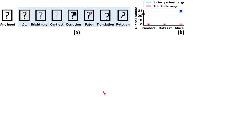
Figure 7. Visualization of the minimal globally robust bounds over various perturbations, for MNIST conv1.

Ablation study

Lastly, we study the importance of VHAGaR’s components via an ablation study. We compare VHAGaR to two variants: MIP-only and MIP + dependencies (i.e., without the hyper-adversarial attack). We run all approaches over the MNIST 3x50 PGD and $conv1$ networks and various perturbation types, for every pair of classes $c^{\prime}$ and $c_{t}$, for 3 hours. We measure the execution time in minutes $t$, the upper bound $\delta^{u}$, and the lower bound $\delta^{l}$. We also measure the minute at which the first non-trivial lower bound is obtained $t^{i}$ and its corresponding class confidence $\delta^{i}$. Note that the first non-trivial lower bound depends on the variant’s MIP (i.e., with/without dependencies, with/without the hyper-adversarial attack’s lower bound). The higher the $\delta^{i}$ the closer the optimization is to the maximal globally non-robust bound, while the shorter the $t^{i}$ the more efficient the variant is. Table 4 shows the results. Our results indicate that VHAGaR is 1.7x faster than the MIP + dependencies variant and 78.6x faster than the MIP-only variant. Given 3 hours, the upper and lower bounds of VHAGaR are identical to the MIP + dependencies variant. The lower bound of the MIP-only variant is smaller by 1.3x and the upper bound is greater by 1.05x. Also, the results show that Algorithm 2 allows VHAGaR to obtain 1.2x (1.5x) higher initial solutions in 6.7x (52.6x) less time compared to the MIP + dependencies variant (MIP-only variant).

Table 4. Ablation study. First two rows are over MNIST 3x50 PGD; the rest are over MNIST $conv1$.

Perturbation	VHAGaR					Our MIP + dependencies					Our MIP
	$t$	$t^{i}$	$\delta^{l}$	$\delta^{u}$	$\delta^{i}$	$t$	$t^{i}$	$\delta^{l}$	$\delta^{u}$	$\delta^{i}$	$t$	$t^{i}$	$\delta^{l}$	$\delta^{u}$	$\delta^{i}$
	$[m]$	$[m]$	$\%$	$\%$	$\%$	$[m]$	$[m]$	$\%$	$\%$	$\%$	$[m]$	$[m]$	$\%$	$\%$	$\%$
Brightness([0,1])	4.8	0.1	48	48	39	8.2	1.2	48	48	30	18.5	1	48	48	27
Brightness([0,0.1])	9.2	0.2	21	21	15	18	1	21	21	12	34.6	1.1	21	21	15
Brightness([0,1])	44	0.7	44	44	36	53	6.5	44	44	31	91	12	44	49	23
Occ.(14,14,3)	0.9	0.15	9	9	7	0.9	0.3	9	9	6	180	40	4	24	3
Pa.([0,1],14,14,[1,3])	0.7	0.05	13	13	6	0.9	0.1	13	13	5	180	0.1	13	34	4
Translation(3,3)	0.1	0.01	93	93	90	0.3	0.1	93	93	67	0.5	0.1	93	93	66

7. Related Work

Global robustness

Several works analyze global robustness properties. Katz et al. (2017); Wang et al. (2022a, b) compute the worst-case change in a network’s outputs but cannot determine whether the classification changes. Ruan et al. (2019); Bastani et al. (2016) estimate global robustness for classifiers from local robustness guarantees. Mangal et al. (2019); Levy et al. (2023) provide probabilistic guarantees. Leino et al. (2021); Zhang et al. (2022a) train $L_{\infty}$ globally robust networks using Lipschitz bounds. Sun et al. (2022) are similar but focus on SDN (and not DNN). Chen et al. (2021) propose booster-fixer training for security classifiers to enforce global robustness. Gopinath et al. (2018) compute robustness guarantees for input regions derived from the dataset, however these do not imply global robustness for any input.

Multiple network encoding

VHAGaR encodes two copies of a network classifier to analyze the output of an input and its perturbed example. Several works employed a similar concept. Katz et al. (2017); Wang et al. (2022a, b) analyze global robustness by reasoning about two copies of a network (not a classifier) and bounding the maximum change in the output caused by an input perturbation. Wang et al. (2022a, b) leverage dependencies defined by delta variables which capture the difference of respective neurons to overapproximate their functionality. In contrast, VHAGaR integrates dependencies stemming from feature perturbations or by solving suitable MIP problems. Other works reason about multiple networks in the context of differential analysis (Mohammadinejad et al., 2021) or local robustness of an ensemble of networks (Yang et al., 2022).

Attack-guided verification

VHAGaR executes a hyper-adversarial attack to obtain suboptimal feasible solutions. Several works integrate adversarial attacks with verification. Anderson et al. (2019) improve a verifier’s precision by leveraging spurious adversarial examples. Balunovic and Vechev (2020) employ attacks to train networks with provable robustness guarantees. Dimitrov et al. (2022) leverage the PGD attack (Madry et al., 2018) to compute robust adversarial regions.

8. Conclusion

We present VHAGaR for computing the minimal globally robust bound of a neural network classifier, under a given perturbation. VHAGaR encodes the problem as a MIP, over two network copies, which is solved in an anytime manner. VHAGaR reduces the MIP’s complexity by (1) identifying dependencies stemming from the perturbation and the network computation and (2) generalizing adversarial attacks to unknown inputs to compute suboptimal lower bounds and optimization hints. Our results show that VHAGaR computes 82.2x tighter bounds and is 130.6x faster than an existing global robustness verifier. Additionally, its lower bounds are 18.8x higher than those computed by sampling approaches. Finally, we exemplify how VHAGaR can provide insights into the robustness attributes of a network classifier to adversarial attacks.

Data-Availability Statement

Our code is available at https://github.com/ananmkabaha/VHAGaR.git.

Appendix A Image Rotation with Bilinear Interpolation

Algorithm 3 shows the standard rotation algorithm that VHAGaR relies on.

Input: An input image $x\in[0,1]^{d_{1}\times d_{2}}$ and a rotation angle $\theta\in[0,2\pi]$.

Output: The rotated image $x_{R}\in[0,1]^{d_{1}\times d_{2}}$.

1 $center=[d_{1}/2+1,d_{2}/2+1]$

2 for $i\in\{1,\dots,d_{1}\}$, $j\in\{1,\dots,d_{2}\}$  do

3       $i_{c}=i-center[1]$

4       $j_{c}=j-center[2]$

5       $i_{r}=(i_{c}\cdot\sin(\frac{\theta\cdot\pi}{180})+j_{c}\cdot\cos(\frac{\theta\cdot\pi}{180}))+center[1]$

6       $j_{r}=(i_{c}\cdot\cos(\frac{\theta\cdot\pi}{180})-j_{c}\sin(\frac{\theta\cdot\pi}{180})+center[2]$

7       if $\lfloor i_{r}\rfloor\geq 1$ and $\lceil i_{r}\rceil\leq d_{1}$ and $\lfloor j_{r}\rfloor\geq 1$ and $\lceil j_{r}\rceil\leq d_{2}$ then

8             $di=i_{r}-\lfloor i_{r}\rfloor$

9             $dj=j_{r}-\lfloor j_{r}\rfloor$

10             $x_{R}[i,j]=(1-di)\cdot(1-dj)\cdot x[\lfloor i_{r}\rfloor,\lfloor j_{r}\rfloor]+di\cdot(1-dj)\cdot x[\lceil i_{r}\rceil,\lfloor j_{r}\rfloor]+(1-di)\cdot dj\cdot x[\lfloor i_{r}\rfloor,\lceil j_{r}\rceil]+di\cdot dj\cdot x[\lceil i_{r}\rceil,\lceil j_{r}\rceil]$

11      

return $x_{R}$

Algorithm 3 Image_Rotation_with_Bilinear_Interpolation($x$, $\theta$)

Appendix B Additional Results

LABEL:tab:add_res provides additional results comparing VHAGaR to the baselines. Figure 8 shows the execution time of VHAGaR’s components: the concrete bound computation, the computation of the dependency constraint, the hyper-adversarial attack, and the time to solve the main MIP (Problem 4). The pie charts show the execution times of the different components as if they run sequentially, however VHAGaR runs the hyper-adversarial attack in parallel to the concrete bound computation and the dependency constraint computation. Additionally, the concrete bound computation and the dependency constraint computation are run once and not separately for each $c_{t}\in C_{t}$. Results show that the dominant factor of VHAGaR’s execution time is solving Problem 4, while the other computations terminate within two minutes combined.

Table 5. Additional results: VHAGaR vs. sampling baselines and Marabou. Sa. abbreviates Sampling, Occ. Occlusion, Pa. Patch, and Trans. Translation. NA is not applicable.

Model	Perturbation	VHAGaR			Marabou			Dataset Sa.		Random Sa.
		$\delta^{l}$	$\delta^{u}$	$t$	$\delta^{l}$	$\delta^{u}$	$t$	$\delta^{DS}$	$t$	$\delta^{RS}\pm h$	$t$
		%	%	$[m]$	%	%	$[m]$	%	$[m]$	%	$[m]$
MNIST	$L_{\infty}$([0,0.5])	99	99	0.1	87	154	180	57	0.2	$7.5\pm 5.4$	0.2
3x50	Brightness([0,1])	48	49	4.8	31	151	131	17	0.4	$4\pm 0.6$	0.4
PGD	Occ.(14,14,5)	60	60	1.6	51	154	139	16	0.2	$2\pm 0.6$	0.2
$\delta^{m}=3.3$	Occ.(14,14,3)	36	36	5.4	33	160	130	7	0.5	$2\pm 0.6$	0.2
$\delta^{d}=73$%	Occ.(1,1,5)	0.6	2	156	2	152	141	0	0.3	$0.03\pm 0.1$	0.2
	Pa.([0,1],14,14,[1,5])	85	85	0.5	78	160	118	32	0.4	$3\pm 0.4$	0.5
	Pa.([0,1],14,14,[1,3])	61	62	2.1	54	157	121	26	0.4	$5\pm 0.4$	0.5
MNIST	Brightness([0,0.25])	54	55	25	42	137	155	23	0.5	$2\pm 16$	0.6
3x50	Brightness([0,0.1])	36	36	33	27	125	167	18	0.6	$1.7\pm 16$	0.6
$\delta^{m}=2.84$	Contrast([1,2])	3	34	172	NA	NA	NA	0.5	0.6	$1.5\pm 14$	0.6
$\delta^{d}=45$%	Contrast([1,1.5])	3	30	180	NA	NA	NA	0.2	0.5	$1\pm 15$	0.5
MNIST	$L_{\infty}$([0,0.5])	98	98	1.2	1	207	180	24	0.3	$2.9\pm 0.3$	0.2
$conv1$	Brightness([0,1])	43	44	44	22	155	180	8	0.8	$2.1\pm 1.1$	0.2
$\delta^{m}=39$	Occ.(14,14,5)	20	20	0.4	0.6	215	180	4	0.6	$0.8\pm 1.1$	0.3
$\delta^{d}=30$%	Occ.(14,14,3)	9	9	0.9	17	151	180	1	0.6	$0.5\pm 1.1$	0.3
	Occ.(1,1,9)	24	25	0.2	6	233	180	1	0.6	$1.3\pm 0.7$	0.2
	Pa.([0,1],1,1,[1,9])	36	37	0.3	2	211	180	11	0.4	$3.1\pm 1.0$	0.5
	Pa.([0,1],1,1,[1,5])	10	11	0.7	33	155	180	4	0.4	$1.1\pm 1.0$	0.5
	Trans.(0,[1,3])	90	90	1.5	21	155	180	15	0.4	$2.0\pm 1.5$	0.4
	Trans.([1,3],0)	90	92	1.8	17	191	180	19	0.5	$2.3\pm 1.3$	0.4
	Rotation($1^{\circ}$)	71	74	1.4	24	187	180	8	1.6	$0.7\pm 0.5$	1.2
	Rotation($5^{\circ}$)	77	80	1.2	31	211	180	9	1.4	$0.9\pm 0.6$	1.3
MNIST	$L_{\infty}$([0,0.1])	49	50	2.4	0	305	180	8	0.3	$1.5\pm 0.03$	0.2
$conv2$	Brightness([0,1])	36	38	55	3	595	180	11	0.6	$0.5\pm 0.03$	0.3
$\delta^{m}=147$	Occ.(14,14,9)	40	40	1.1	0	310	180	10	1.4	$0.4\pm 0.06$	0.3
$\delta^{d}=42$%	Occ.(14,14,3)	8	8	2.5	0	303	180	2	1.4	$0.1\pm 0.06$	0.3
	Occ.(1,1,9)	28	29	1.2	0	324	180	3	1.3	$0.6\pm 0.06$	0.3
	Pa.([0,1],1,1,[1,9])	45	45	0.9	0	301	180	12	0.4	$0.7\pm 0.02$	0.4
	Pa.([0,1],1,1,[1,5])	3	3	1.6	0	304	180	1	0.5	$0.3\pm 0.03$	0.4
	Trans.(0,[1,3])	90	91	0.8	0	303	180	19	0.3	$1.1\pm 0.02$	0.3
	Trans.([1,3],0)	87	87	1	0	304	180	24	0.4	$0.7\pm 0.03$	0.4
	Rotation($1^{\circ}$)	59	61	2.1	0	536	180	10	1.2	$0.5\pm 0.06$	0.9
	Rotation($5^{\circ}$)	61	62	2.1	0	631	180	11	1.2	$0.6\pm 0.08$	1.0
FMNIST	Brightness([0,1])	47	64	180	37	225	180	6	0.3	$0.6\pm 0.1$	0.6
$conv1$	Brightness([0,0.25])	32	56	162	26	195	180	3	0.3	$0.55\pm 0.1$	0.6
$\delta^{m}=66.8$	Occ.(14,14,5)	13	13	4.2	12	151	180	2	0.6	$0.15\pm 0.1$	0.4
$\delta^{d}=46$%	Occ.(14,14,3)	7	7	4.8	6	153	180	0.5	0.6	$0.07\pm 0.1$	0.4
	Occ.(1,1,5)	17	17	2.9	15	151	180	0.2	0.5	$0.3\pm 0.15$	0.4
	Pa.([0,1],1,1,[1,9])	69	70	0.6	63	151	180	8	0.2	$0.6\pm 0.05$	0.5
	Pa.([0,1],1,1,[1,5])	28	28	4.7	25	156	180	4	0.2	$0.7\pm 0.1$	0.5
	Trans.(0,[1,3])	89	89	7.9	87	151	180	14	0.3	$1.0\pm 0.1$	0.2
	Trans.([1,3],0)	91	92	8.6	84	156	180	12	0.5	$0.65\pm 0.2$	0.2
	Rotation($1^{\circ}$)	80	81	5	70	154	180	6	1.8	$0.7\pm 0.2$	1.2
	Rotation($5^{\circ}$)	85	86	4.5	75	153	180	7	1.6	$0.9\pm 0.15$	1.2
CIFAR10	Occ.(14,14,9)	31	48	85	0	317	180	7	0.3	$0.7\pm 0.3$	0.3
$conv1$	Occ.(14,14,5)	16	25	46	0	307	180	3	0.3	$0.6\pm 0.3$	0.3
$\delta^{m}=54.3$	Occ.(14,14,3)	9	16	54	0	301	180	1	0.2	$0.4\pm 0.3$	0.3
$\delta^{d}=43$%	Pa.([0,1],1,1,[1,9])	42	43	13	1	301	180	6	0.5	$1.0\pm 0.1$	0.5
	Pa.([0,1],1,1,[1,5])	25	27	24	0	313	180	2	0.5	$0.6\pm 0.2$	0.5

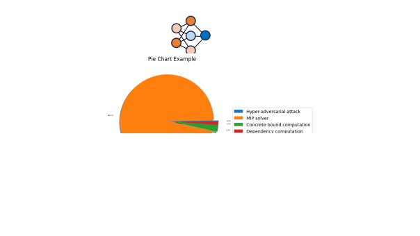
Figure 8. Execution time of VHAGaR’s different components.

References

- (1)
- Alfarra et al. (2020) Motasem Alfarra, Adel Bibi, Hasan Hammoud, Mohamed Gaafar, and Bernard Ghanem. 2020. On the Decision Boundaries of Neural Networks: A Tropical Geometry Perspective. In abs/2002.08838 (2020).
- Anderson et al. (2019) Greg Anderson, Shankara Pailoor, Isil Dillig, and Swarat Chaudhuri. 2019. Optimization and abstraction: a synergistic approach for analyzing neural network robustness. In PLDI (2019).
- Balunovic et al. (2019) Mislav Balunovic, Maximilian Baader, Gagandeep Singh, Timon Gehr, and Martin T. Vechev. 2019. Certifying Geometric Robustness of Neural Networks. In NeurIPS (2019).
- Balunovic and Vechev (2020) Mislav Balunovic and Martin T. Vechev. 2020. Adversarial Training and Provable Defenses: Bridging the Gap. In ICLR (2020).
- Bastani et al. (2016) Osbert Bastani, Yani Ioannou, Leonidas Lampropoulos, Dimitrios Vytiniotis, Aditya V. Nori, and Antonio Criminisi. 2016. Measuring Neural Net Robustness with Constraints. In NeurIPS (2016).
- Bhattad et al. (2020) Anand Bhattad, Min Jin Chong, Kaizhao Liang, Bo Li, and David A. Forsyt. 2020. Unrestricted Adversarial Examples via Semantic Manipulation. In ICLR (2020).
- Carlini and Wagner. (2017) Nicholas Carlini and David A. Wagner. 2017. Towards Evaluating the Robustness of Neural Networks. In SP (2017).
- Chen et al. (2018) Pin-Yu Chen, Yash Sharma, Huan Zhang, Jinfeng Yi, and Cho-Jui Hsieh. 2018. EAD: Elastic-Net Attacks to Deep Neural Networks via Adversarial Examples. In AAAI (2018).
- Chen et al. (2017) Pin-Yu Chen, Huan Zhang, Yash Sharma, Jinfeng Yi, and Cho-Jui Hsieh. 2017. ZOO: Zeroth Order Optimization Based Black-box Attacks to Deep Neural Networks without Training Substitute Models. In AISec Workshop (2017).
- Chen et al. (2021) Yizheng Chen, Shiqi Wang, Yue Qin, Xiaojing Liao, Suman Jana, and David A. Wagner. 2021. Learning Security Classifiers with Verified Global Robustness Properties. In CCS (2021).
- Dimitrov et al. (2022) Dimitar Iliev Dimitrov, Gagandeep Singh, Timon Gehr, and Martin T. Vechev. 2022. Provably Robust Adversarial Examples. In ICLR (2022).
- Ehlers (2017) Rüdiger Ehlers. 2017. Formal verification of piece-wise linear feed-forward neural networks. In ATVA (2017).
- Engstrom et al. (2019) Logan Engstrom, Brandon Tran, Dimitris Tsipras, Ludwig Schmidt, and Aleksander Madry. 2019. Exploring the Landscape of Spatial Robustness. In ICML (2019).
- Engstrom et al. (2017) Logan Engstrom, Dimitris Tsipras, Ludwig Schmidt, and Aleksander Madry. 2017. A Rotation and a Translation Suffice: Fooling CNNs with Simple Transformations. In abs/1712.02779 (2017).
- Goodfellow et al. (2015) Ian J. Goodfellow, Jonathon Shlens, and Christian Szegedy. 2015. Explaining and Harnessing Adversarial Examples. In ICLR (2015).
- Gopinath et al. (2018) Divya Gopinath, Guy Katz, Corina S. Pasareanu, and Clark W. Barrett. 2018. DeepSafe: A Data-Driven Approach for Assessing Robustness of Neural Networks. In ATVA (2018).
- Goswami et al. (2018) Gaurav Goswami, Nalini K. Ratha, Akshay Agarwal, Richa Singh, and Mayank Vatsa. 2018. Unravelling Robustness of Deep Learning based Face Recognition Against Adversarial Attacks. In AAAI (2018).
- He et al. (2016) Kaiming He, Xiangyu Zhang, Shaoqing Ren, and Jian Sun. 2016. Deep Residual Learning for Image Recognition. In IEEE Conference on Computer Vision and Pattern Recognition, CVPR. IEEE Computer Society, 770–778.
- Hoeffding (1963) W. Hoeffding. 1963. Probability inequalities for sums of bounded random variables. J. Amer. Statist. Assoc. 58, 301 (1963), 13–30.
- Huang (2020) Changcun Huang. 2020. ReLU Networks Are Universal Approximators via Piecewise Linear or Constant Functions. In Neural Computation 32, 11 (11 2020), 2249–2278.
- Kabaha and Drachsler-Cohen (2022) Anan Kabaha and Dana Drachsler-Cohen. 2022. Boosting Robustness Verification of Semantic Feature Neighborhoods. In SAS (2022).
- Kabaha and Drachsler-Cohen (2023) Anan Kabaha and Dana Drachsler-Cohen. 2023. Maximal Robust Neural Network Specifications via Oracle-Guided Numerical Optimization. In VMCAI (2023).
- Katz et al. (2017) Guy Katz, Clark W. Barrett, David L. Dill, Kyle Julian, and Mykel J. Kochenderfer. 2017. Reluplex: An Efficient SMT Solver for Verifying Deep Neural Networks. In CAV (2017).
- Katz et al. (2019) Guy Katz, Derek A. Huang, Duligur Ibeling, Kyle Julian, Christopher Lazarus, Rachel Lim, Parth Shah, Shantanu Thakoor, Haoze Wu, Aleksandar Zeljic, David L. Dill, Mykel J. Kochenderfer, and Clark W. Barrett. 2019. The Marabou Framework for Verification and Analysis of Deep Neural Networks. In CAV (2019).
- Krizhevsky (2009) Alex Krizhevsky. 2009. Learning Multiple Layers of Features from Tiny Images. In CoRR, abs/1708.07747 (2009).
- Lecun et al. (1998) Y. Lecun, L. Bottou, Y. Bengio, and P. Haffner. 1998. Gradient-based Learning Applied to Document Recognition. In Proceedings of the IEEE 1998;86(11):2278e324 (1998).
- Leino et al. (2021) Klas Leino, Zifan Wang, and Matt Fredrikson. 2021. Globally-Robust Neural Networks. In ICML (2021).
- Levy et al. (2023) Natan Levy, Raz Yerushalmi, and Guy Katz. 2023. gRoMA: a Tool for Measuring Deep Neural Networks Global Robustness. In arXiv.2301.02288 (2023).
- Liu et al. (2019) Xin Liu, Huanrui Yang, Ziwei Liu, Linghao Song, Yiran Chen, and Hai Li. 2019. DPATCH: An Adversarial Patch Attack on Object Detectors. In AAAI (2019).
- Madry et al. (2018) Aleksander Madry, Aleksandar Makelov, Ludwig Schmidt, Dimitris Tsipras, and Adrian Vladu. 2018. Towards Deep Learning Models Resistant to Adversarial Attacks. In ICLR (2018).
- Mangal et al. (2019) Ravi Mangal, Aditya V. Nori, and Alessandro Orso. 2019. Robustness of neural networks: a probabilistic and practical approach. In ICSE (2019).
- Mohammadinejad et al. (2021) Sara Mohammadinejad, Brandon Paulsen, Jyotirmoy V. Deshmukh, and Chao Wang. 2021. DiffRNN: Differential Verification of Recurrent Neural Networks. In FORMATS (2021).
- Mohapatra et al. (2020) Jeet Mohapatra, Tsui-Wei Weng, Pin-Yu Chen, Sijia Liu, and Luca Daniel. 2020. Towards Verifying Robustness of Neural Networks Against A Family of Semantic Perturbations. In CVPR (2020).
- Qin et al. (2019) Chongli Qin, Krishnamurthy (Dj) Dvijotham, Brendan O’Donoghue, Rudy Bunel, Robert Stanforth, Sven Gowal, Jonathan Uesato, Grzegorz Swirszcz, and Pushmeet Kohli. 2019. Verification of Non-Linear Specifications for Neural Networks. In ICLR (2019).
- Ruan et al. (2019) Wenjie Ruan, Min Wu, Youcheng Sun, Xiaowei Huang, Daniel Kroening, and Marta Kwiatkowska. 2019. Global Robustness Evaluation of Deep Neural Networks with Provable Guarantees for the Hamming Distance. In IJCAI (2019).
- Singh et al. (2019a) Gagandeep Singh, Rupanshu Ganvir, Markus Püschel, and Martin T. Vechev. 2019a. Beyond the Single Neuron Convex Barrier for Neural Network Certification. In NeurIPS (2019).
- Singh et al. (2019b) Gagandeep Singh, Timon Gehr, Markus Püschel, and Martin T. Vechev. 2019b. An abstract domain for certifying neural networks. In POPL (2019).
- Singh et al. (2019c) Gagandeep Singh, Timon Gehr, Markus Püschel, and Martin T. Vechev. 2019c. Boosting Robustness Certification of Neural Networks. In ICLR (2019).
- Sun et al. (2022) Weidi Sun, Yuteng Lu, Xiyue Zhang, and Meng Sun. 2022. DeepGlobal: A framework for global robustness verification of feedforward neural networks. In J. Syst. Archit. (2022).
- Szegedy et al. (2014) Christian Szegedy, Wojciech Zaremba, Ilya Sutskever, Joan Bruna, Dumitru Erhan, Ian J. Goodfellow, and Rob Fergus. 2014. Intriguing Properties of Neural Networks. In ICLR (2014).
- Tjeng et al. (2019) Vincent Tjeng, Kai Y. Xiao, and Russ Tedrake. 2019. Evaluating robustness of neural networks with mixed integer programming. In ICLR (2019).
- Tu et al. (2019) Chun-Chen Tu, Pai-Shun Ting, Pin-Yu Chen, Sijia Liu, Huan Zhang, Jinfeng Yi, Cho-Jui Hsieh, and Shin-Ming Cheng. 2019. AutoZOOM: Autoencoder-Based Zeroth Order Optimization Method for Attacking Black-Box Neural Networks. In AAAI (2019).
- Wang et al. (2018) Shiqi Wang, Kexin Pei, Justin Whitehouse, Junfeng Yang, and Suman Jana. 2018. Efficient Formal Safety Analysis of Neural Networks. In NeurIPS (2018).
- Wang et al. (2021) Shiqi Wang, Huan Zhang, Kaidi Xu, Xue Lin, Suman Jana, Cho-Jui Hsieh, and J Zico Kolter. 2021. Beta-CROWN: Efficient Bound Propagation with Per-neuron Split Constraints for Neural Network Robustness Verification. In NeurIPS (2021).
- Wang et al. (2022a) Zhilu Wang, Chao Huang, and Qi Zhu. 2022a. Efficient Global Robustness Certification of Neural Networks via Interleaving Twin-Network Encoding. In DATE 2022 (2022).
- Wang et al. (2022b) Zhilu Wang, Yixuan Wang, Feisi Fu, Ruochen Jiao, Chao Huang, Wenchao Li, and Qi Zhu. 2022b. A Tool for Neural Network Global Robustness Certification and Training. In https://doi.org/10.48550/arXiv.2208.07289 2022 (2022).
- Wu et al. (2019) Tong Wu, Liang Tong, and Yevgeniy Vorobeychik. 2019. Defending Against Physically Realizable Attacks on Image Classification. In ICLR (2019).
- Yang et al. (2022) Zhuolin Yang, Linyi Li, Xiaojun Xu, Bhavya Kailkhura, Tao Xie, and Bo Li. 2022. On the Certified Robustness for Ensemble Models and Beyond. In ICLR (2022).
- Zhang et al. (2022a) Bohang Zhang, Du Jiang, Di He, and Liwei Wang. 2022a. Rethinking Lipschitz Neural Networks and Certified Robustness: A Boolean Function Perspective. In NeurIPS (2022).
- Zhang et al. (2020) Chaoning Zhang, Philipp Benz, Tooba Imtiaz, and In So Kweon. 2020. Understanding Adversarial Examples From the Mutual Influence of Images and Perturbations. In CVPR (2020).
- Zhang et al. (2022b) Huan Zhang, Shiqi Wang, Kaidi Xu, Yihan Wang, Suman Jana, Cho-Jui Hsieh, and J. Zico Kolter. 2022b. A Branch and Bound Framework for Stronger Adversarial Attacks of ReLU Networks. In ICML (2022).