Universal quantum computation using quantum annealing with the transverse-field Ising Hamiltonian

Abstract

Quantum computation is a promising emerging technology, and by utilizing the principles of quantum mechanics, it is expected to achieve faster computations than classical computers for specific problems. There are two distinct architectures for quantum computation: gate-based quantum computers and quantum annealing. In gate-based quantum computation, we implement a sequence of quantum gates that manipulate qubits. This approach allows us to perform universal quantum computation, yet they pose significant experimental challenges for large-scale integration. On the other hand, with quantum annealing, the solution of the optimization problem can be obtained by preparing the ground state. Conventional quantum annealing devices with transverse-field Ising Hamiltonian, such as those manufactured by D-Wave Inc., achieving around 5000 qubits, are relatively more amenable to large-scale integration but are limited to specific computations. In this paper, we present a practical method for implementing universal quantum computation within the conventional quantum annealing architecture using the transverse-field Ising Hamiltonian. Our innovative approach relies on an adiabatic transformation of the Hamiltonian, changing from transverse fields to a ferromagnetic interaction regime, where the ground states become degenerate. Notably, our proposal is compatible with D-Wave devices, opening up possibilities for realizing large-scale gate-based quantum computers. This research bridges the gap between conventional quantum annealing and gate-based quantum computation, offering a promising path toward the development of scalable quantum computing platforms.

Usage

Secondary publications and information retrieval purposes.

Structure

You may use the description environment to structure your abstract; use the optional argument of the \item command to give the category of each item.

I Introduction

Quantum computers, utilizing the principles of quantum mechanics, are expected to provide faster computation than classical computers. In the field of quantum computation, two distinctive architectures have emerged: gate-based quantum computers and quantum annealing, each offering unique approaches to harnessing quantum phenomena [1, 2, 3].

The gate-based quantum computer consists of sequential unitary quantum gates, enabling universal quantum computation. In particular, we remark that arbitrary unitary quantum gates can be constructed by combining several types of unitary gates, called universal gate sets[4, 5, 6, 7]. Typically, either phase accumulation (such as Ramsey interferometry) or application of an oscillating field (such as Rabi oscillations) is adopted to implement the gate operations for a solid-state quantum computer. It has the potential for a wide array of applications, including quantum chemistry, machine learning, financial engineering, optimization problems, and decrypting ciphers[8, 9, 10, 6, 11, 12]. Most quantum algorithms to achieve quantum speed-up need quantum error collection, exemplified by a surface code[13]. This paradigm, known as fault-tolerant quantum computation(FTQC), requires thousands of physical qubits per logical qubit to effectively suppress the noise effect. Consequently, it is estimated that FTQC will at least require 10 million qubits to perform computations beyond the capabilities of existing classical computers. Nevertheless, the scalability of gate-based quantum computers poses substantial experimental challenges, limiting them to utilizing only around a hundred qubits with current technology.

In contrast to gate-based quantum computation, quantum annealing(QA) offers an alternative method, focused on solving combinatorial optimization problems by preparing the ground state of an Ising Hamiltonian. Quantum annealers with transverse-field Ising Hamiltonians, such as those developed by D-Wave Systems, have made thousands of qubits available for these tasks[14, 15]. QA has many applications besides solving combinatorial optimization problems, such as machine learning[16, 17, 18, 19, 20, 21, 22, 23, 24, 25, 26, 27] and physical simulation[28, 29, 30, 31, 32]. QA can perform adiabatic time evolution for a sufficiently long time, and then find the ground state of the Hamiltonian with high accuracy. Also, the adiabaticity of this process is guaranteed by the adiabatic theorem[33, 34, 35]. Significant efforts have been devoted to achieving adiabaticity in a short time.

Adiabatic quantum computation is an approach to implement universal quantum computation with adiabatic dynamics. [36, 37]. However, adiabatic quantum computation encounters significant challenges. One primary obstacle is the requirement for many ancillary qubits. As the corresponding circuit depth increases, the necessary number of ancillary qubits also increases. Additionally, it necessitates the use of the so-called non-stoquastic Hamiltonian, which is experimentally difficult to realize. The demonstration with the non-stoquastic Hamiltonian was limited to a few qubits.

Various techniques for qubit realization have been proposed, with superconducting qubits emerging as a particularly promising approach. Within this domain, transmons and flux qubits[38, 39, 40, 41] are known as the primary methods for realizing qubits using superconductivity. Flux qubits, which are used in D-Wave devices, are renowned for their scalability without the need for introducing microwaves[15, 14]. However, their application is limited to Quantum annealing(QA) as they cannot perform all universal gate operations. In contrast, transmon qubits despite their integration challenges, are capable of realizing a universal gate set with high fidelity. This capability was notably demonstrated in the experiment conducted by Google Inc. for achieving quantum supremacy. Recently, this scheme using cold atoms in qubit construction has attracted a great deal of attention[42, 43, 44]. This approach is anticipated to have high precision gate operations and long coherence time.

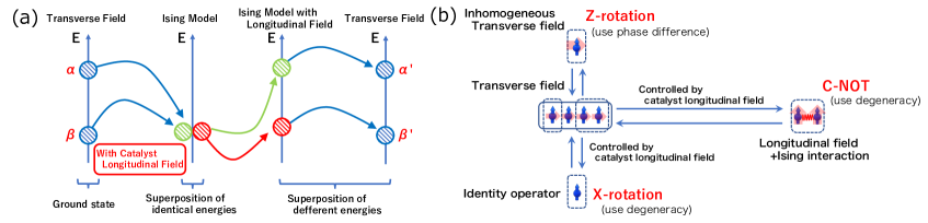
Figure 1: (a)Illustration of our method to implement an $X$ rotation gate. First, we prepare a superposition between the ground and first excited states with the transverse field Hamiltonian. The process initiates with the preparation of an all-plus state, which serves as the ground state of the transverse field. This state is the starting point for implementing quantum annealing with a degenerate Ising model. Second, we decrease the amplitude of the transverse fields while we increase the amplitude of the Ising interaction and longitudinal field. Third, we let the Hamiltonian have degenerate ground states. Fourth, we increase the amplitude of the transverse fields while we decrease the amplitude of the Ising interaction and longitudinal field. Finally, the population of the ground state and first excited state is changed when the Ising interaction and longitudinal field vanishes. (b)Schematic of Gate-Based Quantum Computation Construction. This figure illustrates the comprehensive framework for constructing gate-based quantum computation using our proposed scheme. We regard the center of this figure which is under the transverse magnetic field as the idling state. The X-rotation gate and the controlled-not gate are implemented by the procedures of the section III.3 and the section III.2. On the other hand, the Z-rotation gate is realized in the method described in Section III.4 using the difference of phase. Hence, we can realize the gate-based quantum computation using the transverse Ising model.

In this paper, we present a practice method for implementing universal quantum computation within the conventional quantum annealing architecture using the transverse-field Ising Hamiltonian. Our method relies on an adiabatic transformation of the Hamiltonian, changing from transverse fields to a ferromagnetic interaction regime where the ground states become degenerate. Importantly, the degeneracy provides a way to prepare not only the ground state but also the excited states, which makes it possible to implement the X-gate rotation and controlled-X rotation gate. Unlike the previous approach to realize a solid-state quantum computer, we do not use either the phase accumulation or the application of oscillating fields to implement the X-gate rotation and controlled-X rotation gate. A notable advantage of our method is its independence from microwave pulses, enhancing scalability potential in integrated systems. Moreover, our proposal is compatible with D-Wave devices, opening up prospects for realizing large-scale gate-based quantum computers. This research bridges the gap between quantum annealing and gate-based quantum computation, paving the way for a scalable quantum computing platform.

The rest of this paper is organized as follows. Section II is devoted to a comprehensive review of quantum annealing and universal quantum computation. In Section A, we elucidate the method for adiabatically creating superposition states through degeneracy. In Section III, we introduce gate operation using our scheme. Section IV describes numerical simulations conducted to evaluate the performance of our scheme. In Section V, we perform an experimental demonstration of several gate operations using a D-Wave device. The construction of a gate-based quantum computer using a D-Wave device is Section VI will construct a gate-based quantum computer using a D-Wave device. We conclude with Section VII.

II Review of quantum annealing

Let us review quantum annealing. A solution of the combinatorial optimization problems can be embedded into a ground state of an Ising Hamiltonian $H_{P}$. We can use quantum annealing to find the ground state of an Ising Hamiltonian via adiabatic dynamics. Let us consider a trivial Hamiltonian $H_{D}$, such as transverse fields called the driver Hamiltonian. We define the annealing Hamiltonian as

$$H(t)\equiv\biggl{(}1-\frac{t}{T}\biggr{)}H_{D}+\frac{t}{T}H_{P}.$$ (1)

where $T$ denotes the annealing time. We prepare the ground state of the drive Hamiltonian and let the state evolve by the annealing Hamiltonian in Eq (1) from $t=0$ to $t=T$. A notable aspect of QA is that when an annealing Hamiltonian maintains a certain symmetry, the dynamics is constrained within the same sector by block-diagonalization and QA could fail [2, 45, 46, 47, 48]. Unless such symmetry exists, the quantum adiabatic theorem guarantees that we obtain the ground state of the problem Hamiltonian for a long $T$.

III Realization of gate operation

In this section, we explain how to implement the single-qubit rotation gate and the controlled-not gate by quantum annealing. In our method, when we do not perform any gates, we set the transverse magnetic field Hamiltonian, which we call the idling Hamiltonian. To perform the Z rotation gate, we use the phase accumulation between the ground state and the first excited states. On the other hand, to perform either X-gate rotation or controlled not gate, we adopt a unique approach. Our method consists of two key processes: quantum annealing with a degenerate problem Hamiltonian and reverse annealing. We control the gate operation by adjusting the longitudinal magnetic field during the quantum annealing.

III.1 Change in the amplitude of the superposition of the energy eigenstate of a degenerate Hamiltonian

We describe the method for controlling the amplitude of the superposition of energy eigenstates of the degenerate Hamiltonian. We focus on scenarios where the ground states of the problem Hamiltonian $H_{P}$ are doubly degenerate. The two ground states of the problem Hamiltinian $H_{P}$ are denoted by $\ket{\phi_{1}},\ \ket{\phi_{2}}$. After QA with a sufficiently long $T$, we obtain the following state

$$\ket{\Phi}=\alpha\ket{\phi_{1}}+\sqrt{1-\alpha^{2}}\ket{\phi_{2}}$$ (2)

where $\alpha$ is the amplitude of $\ket{\phi_{1}}$. Importantly, $\alpha$ will be determined by the process of QA.

First, to control the amplitude $\alpha$, we introduce the following ”forward” Hamiltonian

$$H_{F}(t)=\begin{dcases}\Bigl{(}1-\frac{t}{T}\Bigr{)}H_{D}+\frac{t}{T}H_{P}+\frac{t}{T}h_{z}H_{C},&\Bigl{(}t<\frac{T}{2}\Bigr{)}\\ \Bigl{(}1-\frac{t}{T}\Bigr{)}H_{D}+\frac{t}{T}H_{P}+\Bigl{(}1-\frac{t}{T}\Bigr{)}h_{z}H_{C},&\Bigl{(}t>\frac{T}{2}\Bigr{)}\end{dcases}$$ (3)

where $H_{C}$ is the catalytic Hamiltonian and $h_{z}$ is the amplitude parameter of the catalytic term. We should remark that when $h_{z}=0$, this Hamiltonian is identical to the conventional annealing Hamiltonian. Also, the properties $H(t=0)=H_{D}$ and $H(t=T)=H_{P}$ hold independent on amplitude parameter $h_{z}$. We can control the population $\alpha$ in (3) via tuning the amplitude parameter $h_{z}$ in (3). Throughout this paper, we choose the longitudinal magnetic field

$$H_{C}=\sum_{i}^{L}\hat{\sigma}_{i}^{(z)}$$ (4)

as the catalytic Hamiltonian $H_{C}$. We call this procedure which is the control of the amplitude for eigenstates for the forward part. Several superpositions of computational basis are prepared using our scheme. We discuss how to implement specific superpositions in detail in the Appendix A.

Next, we introduce a modified problem Hamiltonian. To resolve the degeneracy of the problem Hamiltonian, we add the longitudinal magnetic field. We call this the modified problem Hamiltonian, which is expressed by $\tilde{H}_{P}$. As we will explain later, the specific form of $\tilde{H}_{P}$ depends on the gate to be implemented.

Finally, we introduce the reverse part to convert the problem Hamiltonian to the drive Hamiltonian. The reverse Hamiltonian is as follows.

$$H_{R}(t)=\frac{t}{T}H_{D}+\biggl{(}1-\frac{t}{T}\biggr{)}\tilde{H}_{P}$$ (5)

We note that we have $H_{R}(t=0)=\tilde{H}_{P}$ and $H_{R}(t=T)=H_{D}$. Thus, the Hamiltonian after the reverse part is a drive Hamiltonian.

In short, our scheme consists of two parts: The forward part and the reverse part. We use the forward part to control the amplitude $\alpha$ using the Hamiltonian in (3). After the forward part, the Hamiltonian is the Ising model and the eigenstates of this Hamiltonian are represented by the computational basis. On the other hand, the reverse part is the operation to return to the drive (idling) Hamiltonian The concept of the forward part and the reverse part is illustrated in Fig.2.

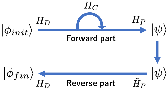
Figure 2: Schematic figure of the Forward and Reverse Parts. In the forward part, our primary objective is to control the amplitude of the degenerated ground states precisely when we finish the forward part. Following the completion of the forward part, the next crucial step involves the addition of a longitudinal magnetic field to the degenerate Ising model. This addition is strategically implemented to resolve the degeneracy that was initially present in the ground states. Finally, we change the Hamiltonian to the transverse magnetic field adiabatically.

III.2 X-rotation gate

To implement the X-rotation gate, the drive Hamiltonian $H_{D}$ is set as the transverse magnetic field as follows

$$H_{D}=-\hat{\sigma}^{(x)}$$ (6)

In addition, we choose

$$H_{P}=-\mbox{1}\mbox{l}$$ (7)

as the problem Hamiltonian. We remark that 1l is represented as the identity operator. We note that the Hamiltonian (7) has degenerated two ground states:$\ket{\uparrow}$ and $\ket{\downarrow}$. Thus, after the forward part, we can control the amplitude of the two ground states. On the other hand, we set the reverse problem Hamiltonian to

$$\tilde{H}_{P}=\hat{\sigma}^{(z)}.$$ (8)

Here, the ground state is $|\downarrow\rangle$ while the first excited state is $|\uparrow\rangle$. After the reverse process, $|\downarrow\rangle$ is changed into $|-\rangle$ while $|\uparrow\rangle$ is changed into $|+\rangle$ as long as the adiabatic condition is satisfied. Therefore, the above process makes the amplitude of each eigenstate $\ket{+}$, $\ket{-}$ controllable using the amplitude parameter $h_{z}$. We discuss this point in the Appendix B.2.1.

We need to adjust a relative phase after we perform the X-rotation gate. For a given initial state of $\alpha|+\rangle+\beta e^{i\theta}|-\rangle$, we obtain $\alpha^{\prime}|+\rangle+\beta^{\prime}e^{i(\theta+\theta^{\prime})}|-\rangle$ after performing the X-rotation gate where $\alpha$, $\beta$, $\alpha^{\prime}$, $\beta^{\prime}$, $\theta$, and $\theta^{\prime}$ are real coefficients. We can control the amplitude of $\alpha^{\prime}$ and $\beta^{\prime}$ by controlling the scheduling of $H_{C}$. On the other hand, we need to apply a Z-rotation gate to change the relative phase from $e^{i(\theta+\theta^{\prime})}$ to $e^{i\theta}$. We can estimate the value of $\theta^{\prime}$ using either numerical simulations or actual experiments. We will explain how to implement the Z-rotation gate later.

III.3 Controlled-not gate

To implement the controlled-not gate operation by using our approach, the drive Hamiltonian is set as the transverse magnetic field as follows.

$$H_{D}=-\hat{\sigma}_{1}^{(x)}-\frac{1}{2}\hat{\sigma}_{2}^{(x)}$$ (9)

The system described in the Hamiltonian (9) does not have any degeneracy. Also, we choose

$$H_{P}=\Bigl{(}\hat{\sigma}_{1}^{(z)}+\mbox{1}\mbox{l}\Bigr{)}\Bigl{(}a\hat{\sigma}_{2}^{(z)}+\mbox{1}\mbox{l}\Bigr{)}$$ (10)

as the problem Hamiltonian, where the parameter a is satisfied with the inequality $0<a<1$. We note that $\ket{\downarrow\downarrow}$ and $\ket{\downarrow\uparrow}$ are degenerated ground states. In addition, $\ket{\uparrow\uparrow}$ and $\ket{\uparrow\downarrow}$ are non-degenerate eigenstates. Thus, the energy spectrum of this problem Hamiltonian is illustrated in Fig 3.

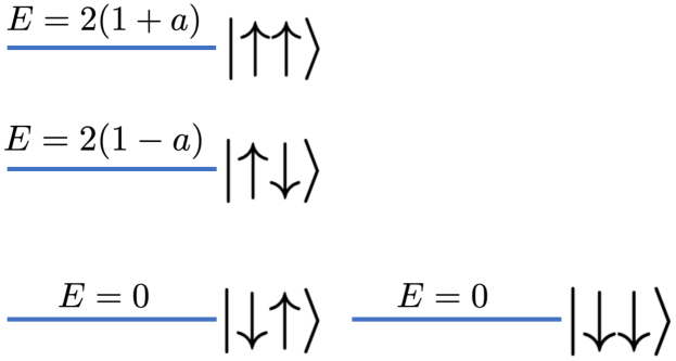
Figure 3: Energy diagram of the problem Hamiltonian for the controlled-not gate. The constant $a$ satisfies the condition $0<a<1$. This figure shows that the $\ket{\downarrow\uparrow}$ and $\ket{\downarrow\downarrow}$ are degenerated ground states and $\ket{\uparrow\uparrow}$ and $\ket{\uparrow\downarrow}$ are non-degenerate excited states.

To implement the reverse part, we choose the reverse problem Hamiltonian as

$$\tilde{H}_{P}=\Bigl{(}b\hat{\sigma}_{1}^{(z)}+\mbox{1}\mbox{l}\Bigr{)}\Bigl{(}a\hat{\sigma}_{2}^{(z)}+\mbox{1}\mbox{l}\Bigr{)}.$$ (11)

We assume that $a<b$ and $0<b<1$ are satisfied. In this case, the order of the energy eigenstates remains the same as that in Fig 4. After the reverse process, $|\downarrow\downarrow\rangle$, $|\downarrow\uparrow\rangle$, $|\uparrow\downarrow\rangle$, and $|\uparrow\uparrow\rangle$ are changed into $|--\rangle$, $|-+\rangle$, $|+-\rangle$, and $|++\rangle$, respectively as long as the adiabatic condition is satisfied. Similar to the case of the X-rotation gate, we need to adjust the relative phase after performing the controlled-not gate. Here, we assume that the interaction between qubits is off when we apply only the transverse magnetic field. Also, we assume that the interaction gradually increases as we decrease the transverse magnetic fields. This assumption is valid for the D-wave cloud system. Due to this assumption, while we perform the controlled-not gate between two qubits, the other qubits are unaffected by the operation.

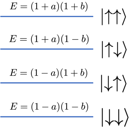
Figure 4: Energy diagram of the problem Hamiltonian $\tilde{H}_{P}$ (11) for the reverse process when we perform a controlled-not gate. For this system, there is no degeneracy.

III.4 Z-axis rotation

We use the longitudinal magnetic field when we implement the Z-axis gate operation. Specifically, by applying the longitudinal magnetic field, an energy difference is given to the two eigenstates, and we can implement the Z-axis rotation by phase difference with the time evolution as follows.

$$e^{i\hat{\sigma}^{(z)}t} \Bigl{(}\alpha\ket{\uparrow}+\beta\ket{\downarrow}\Bigr{)}$$

$$=\alpha e^{it}\ket{\uparrow}+\beta e^{-it}\ket{\downarrow}.$$ (12)

where $\alpha\ket{\uparrow}+\beta\ket{\downarrow}$ is initial state. This method is similar to the Ramsey interferometry.

IV Numerical Simulation

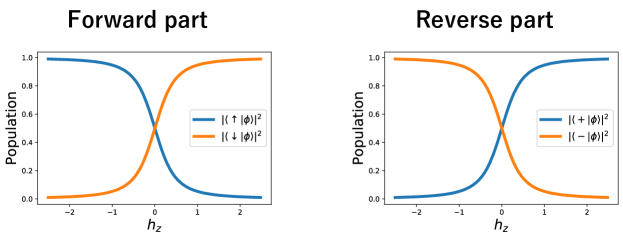
Figure 5: Numerical results of the X-rotation gate with our method. We plot the population of $\ket{\uparrow}$ and $\ket{\downarrow}$ after the forward part of our method. Also, we plot the population of $\ket{-}$ and $\ket{+}$ after the reverse part. After the reverse part, the result shows that we can control the population of $\ket{\uparrow}$ and $\ket{\downarrow}$ by tuning the longitudinal magnetic field $h_{z}$. These results illustrate that we can implement the X-rotation gate with any angle with our method.

In this section, we perform numerical simulations of our method to implement the X rotation and controlled-not gates.

IV.1 X-axis gate

In this subsection, we show the results of the numerical simulations to implement the X-rotation gate of our method. The Hamiltonian $H_{D}$, $H_{P}$, and $\tilde{H}_{P}$ are choosen by (6), (7), and (8), respectively. We adopt the forward Hamiltonian (5) and the reverse Hamiltonian (3) to implement this gate operation. In our simulation, the initial state is set to $\ket{+}$ and the total annealing time $T$ is chosen as $2000$.

We plot the population after the forward part against $h_{z}$ in Fig.5. This plot shows that the populations of $\ket{\uparrow}$ and $\ket{\downarrow}$ are controllable by using the longitudinal magnetic field. Fig.5 (b) shows the population after the reverse part against $h_{z}$. This illustrates that we can choose any populations of $\ket{+}$ and $\ket{-}$ by changing the value of $h_{z}$. Consequently, it is evident that the rotation of the X-axis with any desired rotation angle is feasible within our framework. It is important to note that, for small $T$, the adiabaticity is not guaranteed for both the forward and reverse parts. We discuss how the violation of the adiabaticity affects the dynamics during the implementation of the X-rotation gate in Appendix C. On the other hand, as $T$ approaches $\infty$ in the asymptotic limit, the analytical solution can be derived using perturbation theory. we discuss the result in detail in the Appendix B.

IV.2 Controlled-not gate

In this subsection, we show the results of the numerical simulations of the controlled-not gate with our method. We set the drive Hamiltonian $H_{D}$, the problem Hamiltonian $H_{P}$, and the return problem Hamiltonian $\tilde{H}_{P}$ to be those described in (9), (10), and (11), respectively. Let us assume that the initial state is one of the eigenstates of the driver Hamiltonian. The parameters are chosen as $a=0.3$, $b=0.5$, and $T=20000$. FIG.6 illustrates the population of each eigenstate of the drive Hamiltonian, such as $\ket{++}$, $\ket{+-}$, $\ket{-+}$, and $\ket{--}$, corresponding to each initial state. The first qubit is for control while the second qubit is the target when we perform the controlled-not gate. We can see that if the control qubit is $\ket{+}$, the target qubit undergoes a rotating operation for an arbitrary axis. On the other hand, if the control qubit is $\ket{-}$, the target qubit remains unchanged. Hence, we confirm that the controlled-not operation is successfully implemented with our method. On the other hand, when we decrease the annealing time $T$, the adiabatic condition will be violated, and the controlled-not gate cannot be accurately implemented as shown in the Appendix.C.

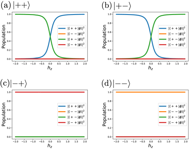
Figure 6: Numerical results of the controlled-not gate with our method. We plot the population of $\ket{++}$, $\ket{+-}$, $\ket{-+}$, and $\ket{--}$ after performing our controlled-not gate. We consider the first (second) qubit as the control (target) qubit. From (a) and (b), if the first qubit is $\ket{+}$, the second qubit is rotated along X axis, and we can tune the rotation angle by changing the strength of the longitudinal magnetic field $h_{z}$. On the other hand, from (c) and (d), if the first qubit is $\ket{-}$, the second qubit is unchanged. These results illustrate that we can implement the controlled-not gate with our method.

V Experimental demonstration

In this section, we show the results to demonstrate our method by using the D-wave device. However, due to a short coherence time, we could not observe the information of the phase in these demonstrations. We observe the population change in the experiments, which is consistent with our theoretical prediction. Also, since we can perform the measurement only when the transverse field is absent with the D-wave device, we perform the experiment only for the forward part of our method. In the D-Wave device, the Hamiltonian is expressed as

$$H(s)= -\frac{A(s)}{2}\biggl{(}\sum_{j}\hat{\sigma}_{j}^{(x)}\biggr{)}$$

$$+\frac{B(s)}{2}\biggl{(}\sum_{j}g(t)h_{j}\hat{\sigma}_{j}^{(z)}+\sum_{i>j}J_{i,j}\hat{\sigma}_{i}^{(z)}\hat{\sigma}_{j}^{(z)}\biggr{)}.$$ (13)

Here, we set $A(s=1)=B(s=0)=0$. The strength of the longitudinal magnetic field $g(t)$ is tunable. Additionally, we can choose the values of the longitudinal magnetic field $\{h_{j}\}_{j}$ and the coupling constant $\{J_{i,j}\}_{i>j}$. Unfortunately, we cannot individually control the longitudinal magnetic field scheduling at each qubit with the current D-wave device. Thus, in this section, we replace uniform longitudinal magnetic field $H_{C}=\sum_{j}\hat{\sigma}_{j}^{{z}}$ in the Section III for the inhomogeneous longitudinal magnetic field $\sum_{j}h_{j}\hat{\sigma}_{j}^{(z)}$. Moreover, we can prepare only the all plus state $\ket{++\cdots+}$ as an initial state in the D-Wave device. It should be noted that we use the D-Wave Advantage system 6.3 for our demonstration.

V.1 Rotation about the X-axis

We experimentally investigate the implementation of the X-rotation gate with our method using the D-wave device. For this purpose, we need to translate the theoretical framework of Subsection III.2 into practical experimentation. To realize the rotation about the X-axis using a single qubit, we set the longitudinal magnetic field as $g(0)=g(T)=0$, $g(T/2)=h_{z}$, and $h_{1}=1$. The initial state is set to be $\ket{\phi}=\ket{+}$. In addition, we set the annealing time as $T=200$, and the measurement number as $N=2000$. Thus, we obtain the plot of the population of $\ket{\uparrow}$ and $\ket{\downarrow}$ against the strength of longitudinal magnetic field $h_{d}$ in the Fig.7.

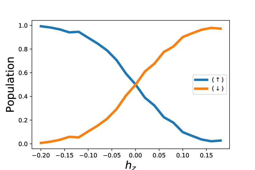
Figure 7: The population of each state against the amplitude parameter of the catalytic term $h_{z}$ when we perform the forward part of our X-rotation gate with the D-wave device. The observed behavior is consistent with our numerical results in Fig.5 and the analytical results in Fig.10.

These experimental results are consistent with our theoretical predictions about the X-rotation gate shown in Fig.5.

V.2 Controlled-not gate using the D-wave device

In this subsection, we experimentally We experimentally investigate the implementation of the X-rotation gate with our method using the D-wave device. The parameters of the problem Hamiltonian are set to $a=0.3$ as defined in the equation (10). Also, the annealing time and the number of measurements are set to be $T=200$ and $N=2000$, respectively. In the equation (13), we set the strength of the longitudinal magnetic fields as $h_{1}=1$, $h_{2}=0.3$, the coupling constant as $J_{12}=0.3$. Also, we set the scheduling of the longitudinal magnetic fields as $g(0)=0$, $g(T/2)=h_{z}+1$, and $g(T)=1$. Due to the constraints of the D-wave device, we can prepare only $\ket{++}$ as the initial state. Furthermore, we cannot apply inhomogeneous transverse magnetic fields with the D-wave device, and so we adopt the homogeneous transverse magnetic field as

$$H_{D}=-\sum_{j=1,2}\hat{\sigma}_{j}^{(x)}.$$ (14)

Notably, the behavior observed in Fig 8 coincides with that of the numerical simulation depicted in Fig.6(a), demonstrating the consistency and effectiveness of our approach.

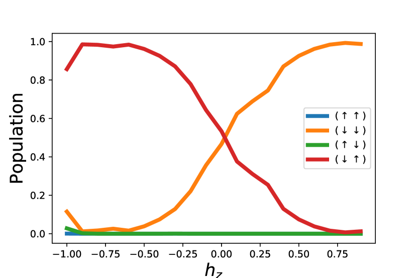
Figure 8: The population of each state against the amplitude parameter of the catalytic term $h_{z}$ when we perform the forward part of the controlled-not gate with the D-wave device. The behavior of this plot corresponds to the analytical solution as shown in Fig.12.

VI Construction of the gate-based quantum computer using D-Wave device

In this section, we construct the gate-based quantum computation using our scheme. Initially, we consider the idling state using the transverse field. To neglect the relative phase, we consider only the case where time is an integer multiple of $2\pi$ divided by the energy gap $k$ as follows.

$$t=\frac{2\pi}{k}n\ \ n\in\mathbb{Z}.$$ (15)

Subsequently, to operate the controlled-not gate and the rotation about the X-axis using previous sections III.2 and III.3, we execute the gate operation through the time evolution between the transverse magnetic field and the Ising model as (7) and (10). When realizing the rotation about the Z-axis the energy difference is controlled by changing the intensity of the transverse magnetic field. The phase difference, as discussed in Section III.4, is utilized to control this energy difference. Finally, we implement repeatedly these gate operations to realize the desired quantum algorithm.

VII Conclusion

In this paper, we propose an innovative approach to implement the controlled-not gate and single-qubit rotation by using a quantum annealer with the transverse-field Ising Hamiltonian. Unlike the previous approach to perform the gate operations by either applying an oscillating field or accumulating a relative phase, we utilize the degenerate ground states to perform the X-rotation gate and controlled-not gate. We demonstrate the effectiveness of our method by numerical simulations and experimental results. Importantly, we do not use microwave pulses to implement gate operations. This feature enhances scalability, as evidenced by the large-scale devices developed by D-Wave Inc. Employing only the transverse-field Ising model, our approach holds substantial promise for developing large-scale gate-based quantum computers.

Appendix A Creation of an arbitrary superposition adiabatically using degeneracy

Here, we explain how to create an arbitrary superposition between degenerated ground states of the problem Hamiltonian. Although we explained a special case that the problem Hamiltonian is the identity in the main text, we will show that the concept introduced in the main text can be generalized to a broader class. Especially, we consider a case where the problem Hamiltonian is the Ising model. The prescription is as follows. First, we adopt the Ising model whose ground states are degenerate and choose this as the problem Hamiltonian. Second, we perform QA where we add a catalytic term of the longitudinal field in the middle of the QA. Finally, we obtain a superposition of the degenerate ground states after QA as long as the adiabatic condition is satisfied. Importantly, if the longitudinal magnetic field is turned on and off during this annealing operation, the amplitude of the superposition between the ground states is controlled.

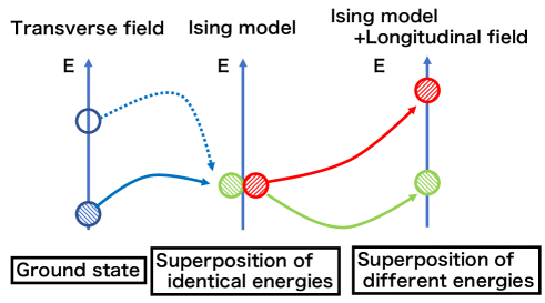
Figure 9: The concept of creation of the superpositioned state. We consider the transverse field as the drive Hamiltonian and, the degenerate Ising model as the problem Hamiltonian. Thus, we obtain the superposition of identical energies when the Hamiltonian is the Ising model. In addition, by adding the longitudinal magnetic field to this Hamiltonian, we obtain the superposition of different energies.

In addition, we introduce several Hamiltonian to have degenerate ground states in the following subsections. Our method can be implementable with the D-wave device.

A.1 Two-state entangled states

We consider the following Ising model as the problem Hamiltonian.

$$H=-\biggl{(}\sum_{i=1}^{N}\alpha_{i}\hat{\sigma}_{i}^{(z)}\biggr{)}^{2},\ \ \alpha_{i}\in\{+1,-1\}.$$ (16)

This Hamiltonian has the following two degenerated ground states.

$$\ket{\Phi}=J_{+}^{(x)}\ket{\downarrow\downarrow\cdots\downarrow},\ J_{-}^{(x)}\ket{\downarrow\downarrow,\cdots\downarrow}$$ (17)

where $J_{+}^{(x)}=\prod_{\alpha_{j}=1}\hat{\sigma}_{j}^{(x)}$, $J_{-}^{(x)}=\prod_{\alpha_{j}=-1}\hat{\sigma}_{j}^{(x)}$. Thus, we can obtain the arbitrary superposition between these two states, including entangled states, via QA as long as adiabatically. For example, we consider the ferromagnetic all-to-all interaction as follows.

$$H=-\biggl{(}\sum_{i=1}^{N}\hat{\sigma}_{i}^{(z)}\biggr{)}^{2}.$$ (18)

where $\alpha_{i}=1$ for all $i$. The ground states of this Hamiltonian are the following.

$$\ket{\uparrow\uparrow\cdots\uparrow},\ket{\downarrow\downarrow\cdots\downarrow}.$$ (19)

Using our proposed method, we can create an arbitrary superposition between these two states.

A.2 Two-state product states

Also, our method is applicable to arbitrary two-state product states. We set the following term as the problem Hamiltonian.

$$H=-\biggl{(}\sum_{i\in A}\alpha_{i}\hat{\sigma}_{i}^{(z)}\biggr{)}^{2}+\biggl{(}\sum_{i\in B}\alpha_{i}\hat{\sigma}_{i}^{(z)}\biggr{)},\ \ \alpha_{i}\in\{+1,-1\}$$ (20)

where $A$, $B$ are denoted by partition of the set $[1,2,\cdots N]$ i.e.

$$A\cap B=\emptyset,A\cup B=[1,2,\cdots,N].$$ (21)

This Hamiltonian has the following two degenerated ground states.

$$\ket{\Phi}=J_{A+}^{(x)}J_{B+}^{(x)}\ket{\downarrow\downarrow\cdots\downarrow},\ J_{A+}^{(x)}J_{B+}^{(x)}J_{A}^{(x)}\ket{\downarrow\downarrow\cdots\downarrow}$$ (22)

where $J_{A}^{(x)}=\prod_{j\in A}\hat{\sigma}_{j}^{(x)}$, $J_{A+}^{(x)}=\prod_{j\in A\land\alpha_{j}=-1}\hat{\sigma}_{j}^{(x)}$, and $J_{B+}^{(x)}=\prod_{j\in B\land\alpha_{j}=-1}\hat{\sigma}_{j}^{(x)}$. Thus, the qubits including the part of $B$ are the same spin states, and, those that include the part of $A$ are different spin states.

For example, we consider the following Hamiltonian as a problem Hamiltonian.

$$H=-\biggl{(}\sum_{i=1}^{N/3}\alpha_{i}\hat{\sigma}_{i}^{(z)}\biggr{)}^{2}+\biggl{(}\sum_{i=N/3+1}^{2N/3}\hat{\sigma}_{i}^{(z)}\biggr{)}+\biggl{(}-\sum_{i=2N/3+1}^{N}\hat{\sigma}_{i}^{(z)}\biggr{)}.$$ (23)

The ground states of this Hamiltonian consist of the superposition of the following two states.

$$\ket{\uparrow\uparrow\cdots\uparrow}_{1:N/3}\ket{\downarrow\downarrow\cdots\downarrow}_{N/3+1:2N/3}\ket{\uparrow\uparrow\cdots\uparrow}_{2N/3+1:1}$$ (24)

$$\ket{\downarrow\downarrow\cdots\downarrow}_{1:N/3}\ket{\uparrow\uparrow\cdots\uparrow}_{N/3+1:2N/3}\ket{\downarrow\downarrow\cdots\downarrow}_{2N/3+1:1}$$ (25)

where $\ket{\uparrow\uparrow\cdots\uparrow}_{a:b}$ is denoted by the state on the $[a,b]$.

Thus, we see that $1\sim N/3$ spins are different and $N/3+1\sim N$ spins are the same, and the ground state is two states that are degenerate; if in superposition, it is a product state.

A.3 The combination of two-state entangled states and product states

We consider combining section A.1 and section A.2 to realize more than three superposition states. We remark that the superposition state obtained by this subsection is a product state. The Hamiltonian which we deal with in this subsection is

$$H=-\sum_{j=1}^{K}\Bigl{(}\sum_{i\in A_{j}}\alpha_{i}\hat{\sigma}_{i}^{(z)}\Bigr{)}^{2}-\biggl{(}\sum_{i\in A_{K+1}}\alpha_{i}\hat{\sigma}_{i}^{(z)}\biggr{)}$$ (26)

where $A_{i}\cap A_{j}=\emptyset$ for $i\neq j$, and $\cup_{j=1}^{K+1}A_{j}=[1,2,\cdots,K+1]$. Here, $\alpha_{i}\in\{+1,-1\}$ is the real coefficient. The degenerate ground states of this Hamiltonian are

$$J_{A_{K+1}+}^{(x)}\prod_{i=1}^{K}\biggl{(}a_{i}+\sqrt{1-a_{i}^{2}}J_{A_{i}}^{(x)}\biggr{)}J_{A_{i}+}^{(x)}\ket{\downarrow\downarrow\downarrow\cdots\downarrow}$$ (27)

where $J_{A_{i}}^{(x)}=\prod_{j\in A_{i}}\hat{\sigma}_{j}^{(x)}$, $J_{A_{i}+}^{(x)}=\prod_{j\in A_{i}\land\alpha_{j}=-1}\hat{\sigma}_{j}^{(x)}$, $J_{A_{K+1}+}^{(x)}=\prod_{j\in A_{K+1}\land\alpha_{j}=-1}\hat{\sigma}_{j}^{(x)}$ and, $a_{i}$ is amplitude of the all down state on the domain $A_{j}$. We can rewrite this state as follows

$$\bigotimes_{j=1}^{K}J_{A_{j}+}^{(x)}\biggl{(} a_{i}\ket{\downarrow\downarrow\cdots\downarrow}_{A_{j}}$$

$$+\sqrt{1-a_{i}^{2}}\ket{\uparrow\uparrow\cdots\uparrow}_{A_{j}}\biggr{)}\otimes J_{A_{K+1}+}^{(x)}\ket{\downarrow\downarrow\cdots\downarrow}_{K+1}$$ (28)

There are $2^{K}$ fold degeneracies for these ground states. Actually, if we take $a_{i}=\pm 1$ for $1,2,\cdots,K$, these states are orthogonal to each other. In this case, we choose $H_{C}$ to apply magnetic fields where the same magnetic fields are applied in the same domain, but different magnetic fields are applied in a different domain.

Although we discussed the case of the Ising model as the problem Hamiltonian, we can generalize this idea to the other model as well. As long as the problem Hamiltonian has the degenerate ground states, a similar discussion can be applied to the other model. The details are left to future work

Appendix B Perturbative analysis of our system

In this appendix, we discuss how the degeneracy of our problem Hamiltonian is resolved by using the perturbative analysis. This elucidates the role of the longitudinal magnetic fields when we implement our method for the gate operations.

B.1 First order perturbation theory formulation for degenerate Hamiltonian

We consider the perturbed Hamiltonian as

$$H=H_{0}+\lambda V$$ (29)

where $H_{0}$ is the unperturbed Hamiltonian, $V$ is the perturbation Hamiltonian, and $\lambda$ is the small perturbation parameter. The perturbative expansion of the eigenenergy and eigenstate is defined by

$$E_{n} =E_{n}^{(0)}+\lambda E_{n}^{(1)}+\lambda^{2}E_{n}^{(2)}\cdots$$ (30)

$$\ket{\phi_{n}} =\ket{\phi_{n}^{(0)}}+\lambda\ket{\phi_{n}^{(1)}}+\lambda^{2}\ket{\phi_{n}^{(2)}}\cdots$$ (31)

where $E_{n}^{(k)}$ is denoted by the $k$-th order perturbation of the $n$-th level eigenenergy and $\ket{\phi_{n}^{(k)}}$ is denoted by $k$-th order perturbation of the $n$-th level eigenstate. We remark that $E_{n}^{(0)}$ ($\ket{\phi_{n}^{0}}$) is eigenenergy(eigenstate) of the perturbed Hamiltonian $H_{0}$.

When the unperturbed Hamiltonian $H_{0}$ has a two-fold degenerate ground state, the $0$-th order eigenstates are given by

$$\ket{\phi_{0}^{(0)}}_{\pm}=c_{\pm,1}\ket{1}+c_{\pm,2}\ket{2}$$ (32)

where $\ket{1}$ and $\ket{2}$ are the ground states of the unperturbed Hamiltonian $H_{0}$ and $c_{\pm,1}$($c_{\pm,2}$) is the amplitude of the $\ket{1}(\ket{0})$. We remark that $c_{+,1}^{*}c_{-,1}+c_{+,2}^{*}c_{-,2}=0$ from orthogonality of the two ground states $\ket{\phi_{0}^{(0)}}_{\pm}$. Also, to satisfy the normalization of the eigenstate, we obtain $|c_{+,1}|^{2}+|c_{+,2}|^{2}=c_{-,1}^{2}+c_{-,2}^{2}=1$. In this case, the perturbation energy formula is given by

$$E_{n,\pm}^{1}=\frac{1}{2}\biggl{\{}(V_{11}+V_{22})\pm\sqrt{(V_{11}-V_{22})^{2}+4|V_{12}|^{2}}\biggr{\}}$$ (33)

and the ratio of superposition is given by

$$\frac{c_{\pm,1}}{c_{\pm,2}}=\frac{V_{12}}{E_{1\pm}-V_{11}}=\frac{E_{1\pm}-V_{22}}{V_{21}}$$ (34)

where $V_{nm}=\bra{n}V\ket{m},\ n,m=1,2$. We note that to obtain the population of each degenerated state, we need only the coefficient of $0$-th order perturbated states (32).

In this case, we regard $H_{P}$ as the unperturbed Hamiltonian $H_{0}$, and $H_{D}+kH_{C}$ as the perturbed Hamiltonian $V$. Also, we consider the eigenstates $\ket{1}$ and $\ket{2}$ in (32) as the two degenerated groundstates written by the computational basis.

B.2 Application of the perturbative analysis to our method

Let us substitute $H_{0}=H_{P}$ and $V=H_{D}+kH_{C}$ where $H_{P}$ is the problem Hamiltonian, $H_{D}$ is the drive Hamiltonian, and $H_{C}$ is the catalytic Hamiltonian in our method. Also, we consider the eigenstates $\ket{1}$ and $\ket{2}$ in (32) as the two degenerated groundstates written by the computational basis.

B.2.1 Perturbative analysis of X-rotation gate

First, we consider our method described in the section III.2. The two degenerated ground states are $\ket{1}$ and $\ket{2}$ as follows.

$$\ket{1} =\ket{\uparrow}$$ (35)

$$\ket{2} =\ket{\downarrow}$$ (36)

We obtain the $V_{nm},\ n,m=1,2$ using the (35), (36) as follows.

$$V_{11} =h_{z}$$ (37)

$$V_{22} =-h_{z}$$ (38)

$$V_{12} =-1$$ (39)

$$V_{21} =-1$$ (40)

In addition, the first-order perturbation energy $E_{0,\pm}^{(1)}$ in Eq. (33) is given by

$$E_{0,\pm}^{(1)}=\pm\sqrt{1+h_{z}^{2}}$$ (41)

The amplitude of the two degenerated ground states is given by

$$\frac{c_{\pm,1}}{c_{\pm,2}}=\frac{1}{h_{z}\mp\sqrt{1+h_{z}^{2}}}.$$ (42)

Using the normalization condition, we obtain the amplitude of $\ket{\uparrow}$ and $\ket{\downarrow}$ of the $0$-th order perturbated ground states as follows.

$$c_{\pm,1}^{2} =\frac{1}{1+(\pm\sqrt{1+h_{z}^{2}}-h_{z})^{2}}.$$ (43)

$$c_{\pm,2}^{2} =\frac{(\pm\sqrt{1+h_{z}^{2}}-h_{z})^{2}}{1+(\pm\sqrt{1+h_{z}^{2}}-h_{z})^{2}}.$$ (44)

We plot the amplitude of the $\ket{\uparrow}$ and $\ket{\downarrow}$ using the equations (43) and (44) as shown in the Fig 10.

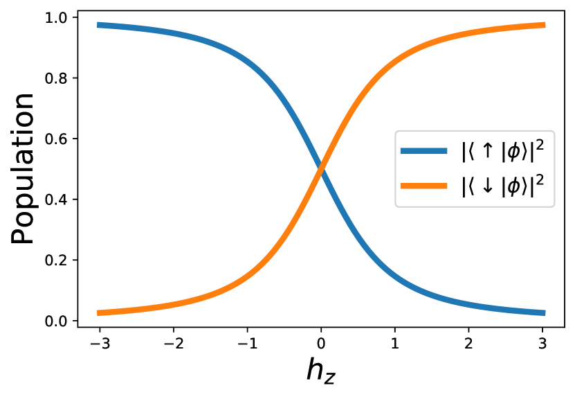
Figure 10: Population of the spin-up state ($\ket{\uparrow}$) and the spin-down state ($|\downarrow\rangle$) after the forward part of the X-rotation gate against $h_{z}$. Here, we adopt the perturbative analysis, and we assume that the initial state is the ground state of the transverse magnetic field$\ket{+}$. We can see that almost all angles of the X-rotation gate by controlling the value of $h_{z}$. Also, we observe that the behavior of this plot qualitatively coincides with the result of numerical simulation in Fig. 5 and experimental simulation using a D-Wave device in Fig. 7.

B.2.2 Perturbative analysis of controlled-not gate operation

Second, we consider the perturbative analysis of the controlled-not gate. From the subsection III.3 in the main text, the degenerated ground states are given by

$$\ket{1} =\ket{\downarrow\downarrow}$$ (45)

$$\ket{2} =\ket{\downarrow\uparrow}.$$ (46)

The drive Hamiltonian is given by the equation (9).

Also, to discuss general circumstances that include the cases in section V and section III as special cases, we consider the inhomogeneous longitudinal magnetic field as follows

$$H_{C}=\hat{\sigma}_{1}+a\hat{\sigma}_{2}.$$ (47)

We remark that in the case where $a=1.0$, the scenario aligns with the formulation presented in section III and the numerical simulation detailed in section IV. On the other hand, when $a=0.3$, the situation corresponds to the experimental results using the D-Wave device discussed in section III. In this case, each transition matrix of the perturbation operator $V_{nm},n,m=1,2$ is given by

$$V_{11} =-(1+a)(1+h_{z})$$ (48)

$$V_{22} =-(a-1)(1+h_{z})$$ (49)

$$V_{12} =-\frac{1}{2}$$ (50)

$$V_{21} =-\frac{1}{2}.$$ (51)

We obtain the first-order perturbation energy $E_{0,\pm}^{(1)}$ as follows.

$$E_{0,\pm}^{(1)}=\frac{1}{2}\biggl{\{}-2(1+h_{z})\pm\sqrt{\Bigl{(}2a(1+h_{z})\Bigr{)}^{2}+1}\biggr{\}}.$$ (52)

Using the (48), (50), (52), and, (34), the ratio $c_{\pm,1}/c_{\pm,2}$ is given by

$$\frac{c_{\pm,1}}{c_{\pm,2}}=\frac{-1}{2a(1+k)\pm\sqrt{(2a(1+k))^{2}+1}}.$$ (53)

Finally, from the normalization of the state $c_{\pm,1}^{2}+c_{\pm,2}^{2}=1$, the population of the $c_{\pm,2}^{2}$ is derived as follows.

$$c_{\pm,1}^{2} =\frac{1}{K^{2}+1},$$ (54)

$$c_{\pm,2}^{2} =\frac{K^{2}}{K^{2}+1}$$ (55)

where

$$K\equiv 2a(1+h_{z})\pm\sqrt{(2a(1+h_{z}))^{2}+1}.$$ (56)

In the inhomogeneous parameter $a=1.0$ we plot the population of the $c_{\pm,1}^{2}$ and $c_{\pm,2}^{2}$ against $h_{z}$ as shown in Fig.11. Also, in the case where $a=0.3$ the population of the $c_{\pm,1}^{2}$ and $c_{\pm,2}^{2}$ against $h_{z}$ for the inhomogeneous parameter $a=1.0$ is ploted as shown in Fig.12.

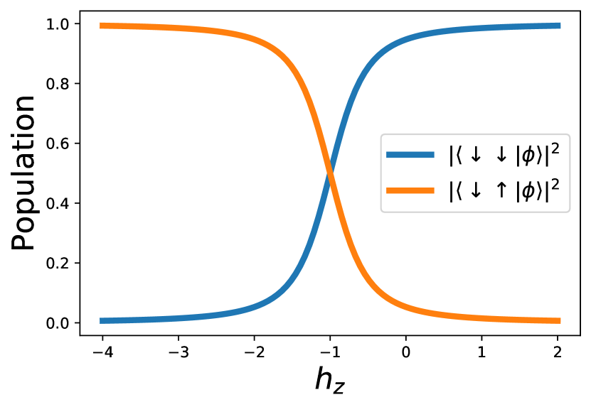
Figure 11: Population of the $\ket{\downarrow\downarrow}$ and $\ket{\downarrow\uparrow}$ after the forward part of the controlled-not gate operation. Here, we adopt the perturbative analysis when parameter $a=1.0$ in the equation (10) and we assume that the initial state is the ground state of the transverse magnetic field$\ket{++}$. It is worth mentioning that this case corresponds to the standard formulation in section.III.3. We observe almost all angles of the controlled-not gate by controlling the value of $h_{z}$.

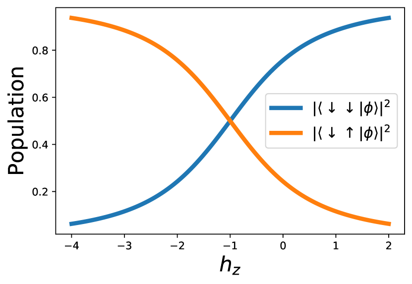
Figure 12: Population of the $\ket{\downarrow\downarrow}$ and $\ket{\downarrow\uparrow}$ after the forward part of the controlled-not gate operation. Here, we use the perturbative analysis when the parameter is $a=0.3$ in the equation (10), and we assume that the initial state is the ground state of the transverse magnetic field$\ket{++}$. It is worth mentioning that this case corresponds to the formulation with the parameter used in the D-wave demonstration in section.V.2. We observe almost all angles of the controlled-not gate by controlling the $h_{z}$.

Appendix C Detail of Result for Numerical simulation

This appendix delves into the comprehensive analysis of the numerical results, elucidating the behaviors observed for both the X-rotation gate and the controlled-not gate operations under varying conditions.

C.1 Rotation about the X-axis

The results for the X-rotation gate, as performed in Section IV.1, are represented in Fig.13. Here, we numerically solve the Schrödinger equation, and we plot the population of the spin-up state and spin-down state against $h_{z}$ after the forward part and reverse part. We confirm that, as we increase $T$, these numerical results converge to the analytical results in Fig.10. Therefore, our approach realizes rotation about the X-axis at any desired angle.

C.2 Controlled-Not gate

We display the results of the numerical simulation for the controlled-not gate in Fig.14 and Fig.15 in detail. The setup is the same as that in the section.V.2. From Fig.14 and Fig.15, we observe that, as we increase $T$, the numerical results approach to the analytical results shown in Fig.11 for the initial state of $\ket{++}$. Moreover, by controlling the value of $h_{z}$, we can control the population of the energy eigenstates after the reverse part when the initial state of the control qubit is $|+\rangle$. Therefore, we can implement the control-not gate with our method.

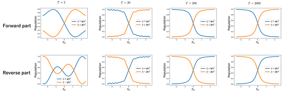
Figure 13: Numerical result of the X-rotation gate after the forward part and the reverse part for several annealing times $T$. These plots show the population after the forward part and the reverse part against the amplitude of the longitudinal magnetic field via forward part $h_{z}$. We choose the upstate $\ket{+}$ as the initial state.

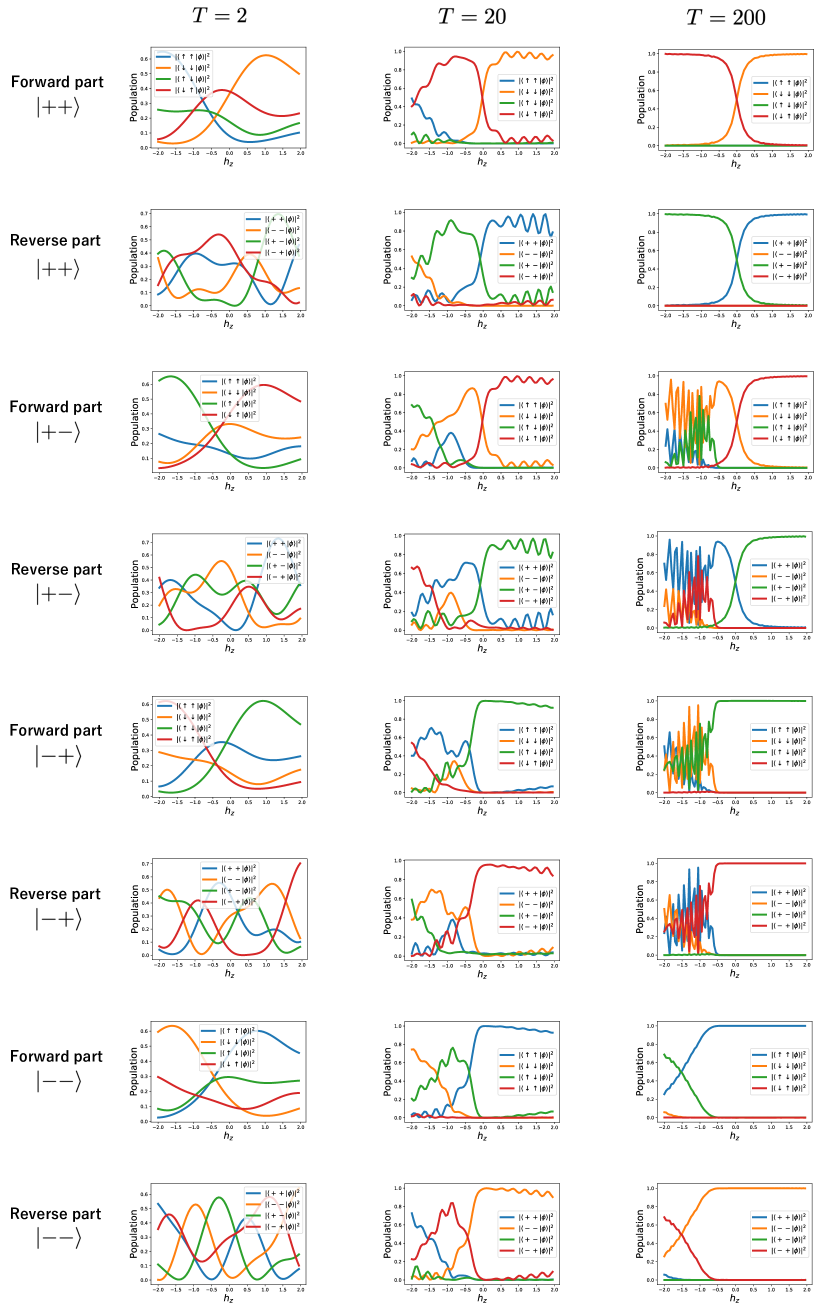
Figure 14: Numerical result of the controlled-not gate after the forward part and the reverse part for annealing time $T=2,20,200$. These plots show the population after the forward part and the reverse part against $h_{z}$ for the several initial states.

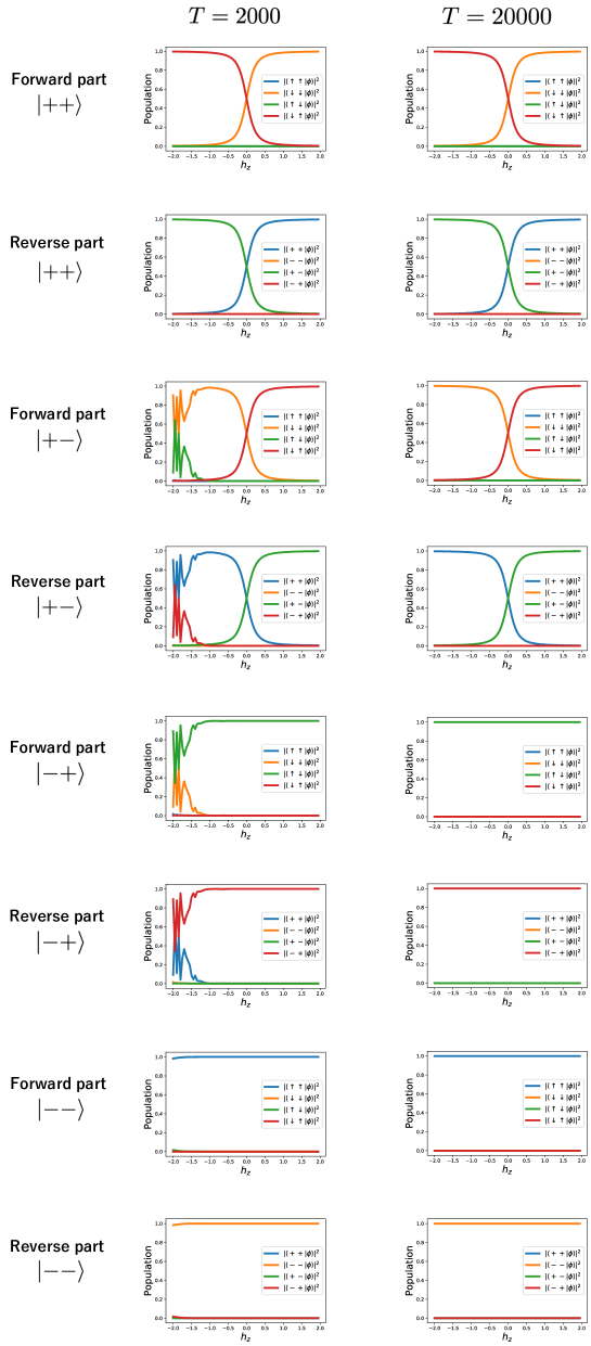
Figure 15: Numerical result of the controlled-not gate after the forward part and the reverse part for annealing time $T=2000,20000$. These plots show the population after the forward part and the reverse part against $h_{z}$ for the several initial states.

References

- Kadowaki and Nishimori [1998] T. Kadowaki and H. Nishimori, Quantum annealing in the transverse ising model, Physical Review E 58, 5355 (1998).
- Farhi et al. [2000] E. Farhi, J. Goldstone, S. Gutmann, and M. Sipser, Quantum computation by adiabatic evolution, arXiv preprint quant-ph/0001106 (2000).
- Farhi et al. [2001] E. Farhi, J. Goldstone, S. Gutmann, J. Lapan, A. Lundgren, and D. Preda, A quantum adiabatic evolution algorithm applied to random instances of an np-complete problem, Science 292, 472 (2001).
- Barenco et al. [1995] A. Barenco, C. H. Bennett, R. Cleve, D. P. DiVincenzo, N. Margolus, P. Shor, T. Sleator, J. A. Smolin, and H. Weinfurter, Elementary gates for quantum computation, Physical review A 52, 3457 (1995).
- Boykin et al. [2000] P. O. Boykin, T. Mor, M. Pulver, V. Roychowdhury, and F. Vatan, A new universal and fault-tolerant quantum basis, Information Processing Letters 75, 101 (2000).
- Kitaev [1995] A. Y. Kitaev, Quantum measurements and the abelian stabilizer problem, arXiv preprint quant-ph/9511026 (1995).
- Shi [2002] Y. Shi, Both toffoli and controlled-not need little help to do universal quantum computation, arXiv preprint quant-ph/0205115 (2002).
- Shor [1994] P. W. Shor, Algorithms for quantum computation: discrete logarithms and factoring, in Proceedings 35th annual symposium on foundations of computer science (Ieee, 1994) pp. 124–134.
- Shor [1999] P. W. Shor, Polynomial-time algorithms for prime factorization and discrete logarithms on a quantum computer, SIAM review 41, 303 (1999).
- Harrow et al. [2009] A. W. Harrow, A. Hassidim, and S. Lloyd, Quantum algorithm for linear systems of equations, Physical review letters 103, 150502 (2009).
- Nielsen and Chuang [2010] M. A. Nielsen and I. L. Chuang, Quantum computation and quantum information (Cambridge university press, 2010).
- Grover [1996] L. K. Grover, A fast quantum mechanical algorithm for database search, in Proceedings of the twenty-eighth annual ACM symposium on Theory of computing (1996) pp. 212–219.
- Kitaev [1997] A. Y. Kitaev, Quantum computations: algorithms and error correction, Russian Mathematical Surveys 52, 1191 (1997).
- Boixo et al. [2014] S. Boixo, T. F. Rønnow, S. V. Isakov, Z. Wang, D. Wecker, D. A. Lidar, J. M. Martinis, and M. Troyer, Evidence for quantum annealing with more than one hundred qubits, Nature physics 10, 218 (2014).
- Johnson et al. [2011] M. W. Johnson, M. H. Amin, S. Gildert, T. Lanting, F. Hamze, N. Dickson, R. Harris, A. J. Berkley, J. Johansson, P. Bunyk, et al., Quantum annealing with manufactured spins, Nature 473, 194 (2011).
- Adachi and Henderson [2015] S. H. Adachi and M. P. Henderson, Application of quantum annealing to training of deep neural networks, arXiv preprint arXiv:1510.06356 (2015).
- Sasdelli and Chin [2021] M. Sasdelli and T.-J. Chin, Quantum annealing formulation for binary neural networks, in 2021 Digital Image Computing: Techniques and Applications (DICTA) (IEEE, 2021) pp. 1–10.
- Date and Potok [2021] P. Date and T. Potok, Adiabatic quantum linear regression, Scientific reports 11, 21905 (2021).
- Wilson et al. [2021] M. Wilson, T. Vandal, T. Hogg, and E. G. Rieffel, Quantum-assisted associative adversarial network: Applying quantum annealing in deep learning, Quantum Machine Intelligence 3, 1 (2021).
- Kumar et al. [2018] V. Kumar, G. Bass, C. Tomlin, and J. Dulny, Quantum annealing for combinatorial clustering, Quantum Information Processing 17, 1 (2018).
- Kurihara et al. [2014] K. Kurihara, S. Tanaka, and S. Miyashita, Quantum annealing for clustering, arXiv preprint arXiv:1408.2035 (2014).
- Willsch et al. [2020] D. Willsch, M. Willsch, H. De Raedt, and K. Michielsen, Support vector machines on the d-wave quantum annealer, Computer physics communications 248, 107006 (2020).
- Heidari et al. [2023] S. Heidari, M. J. Dinneen, and P. Delmas, Quantum annealing for computer vision minimization problems, arXiv preprint arXiv:2312.12848 (2023).
- Woun and Date [2023] D. J. Woun and P. Date, Adiabatic quantum support vector machines, in 2023 IEEE International Conference on Quantum Computing and Engineering (QCE), Vol. 2 (IEEE, 2023) pp. 296–297.
- Neven et al. [2009] H. Neven, V. S. Denchev, G. Rose, and W. G. Macready, Training a large scale classifier with the quantum adiabatic algorithm, arXiv preprint arXiv:0912.0779 (2009).
- Bosch et al. [2023] S. Bosch, B. Kiani, R. Yang, A. Lupascu, and S. Lloyd, Neural networks for programming quantum annealers, arXiv preprint arXiv:2308.06807 (2023).
- Pudenz and Lidar [2013] K. L. Pudenz and D. A. Lidar, Quantum adiabatic machine learning, Quantum information processing 12, 2027 (2013).
- Zhou et al. [2021] S. Zhou, D. Green, E. D. Dahl, and C. Chamon, Experimental realization of classical z 2 spin liquids in a programmable quantum device, Physical Review B 104, L081107 (2021).
- Kairys et al. [2020] P. Kairys, A. D. King, I. Ozfidan, K. Boothby, J. Raymond, A. Banerjee, and T. S. Humble, Simulating the shastry-sutherland ising model using quantum annealing, Prx Quantum 1, 020320 (2020).
- Harris et al. [2018] R. Harris, Y. Sato, A. J. Berkley, M. Reis, F. Altomare, M. Amin, K. Boothby, P. Bunyk, C. Deng, C. Enderud, et al., Phase transitions in a programmable quantum spin glass simulator, Science 361, 162 (2018).
- King et al. [2018] A. D. King, J. Carrasquilla, J. Raymond, I. Ozfidan, E. Andriyash, A. Berkley, M. Reis, T. Lanting, R. Harris, F. Altomare, et al., Observation of topological phenomena in a programmable lattice of 1,800 qubits, Nature 560, 456 (2018).
- King et al. [2023] A. D. King, J. Raymond, T. Lanting, R. Harris, A. Zucca, F. Altomare, A. J. Berkley, K. Boothby, S. Ejtemaee, C. Enderud, et al., Quantum critical dynamics in a 5,000-qubit programmable spin glass, Nature , 1 (2023).
- Kato [1950] T. Kato, On the adiabatic theorem of quantum mechanics, Journal of the Physical Society of Japan 5, 435 (1950).
- Messiah [2014] A. Messiah, Quantum mechanics (Courier Corporation, 2014).
- Jansen et al. [2007] S. Jansen, M.-B. Ruskai, and R. Seiler, Bounds for the adiabatic approximation with applications to quantum computation, Journal of Mathematical Physics 48 (2007).
- Aharonov et al. [2008] D. Aharonov, W. Van Dam, J. Kempe, Z. Landau, S. Lloyd, and O. Regev, Adiabatic quantum computation is equivalent to standard quantum computation, SIAM review 50, 755 (2008).
- Biamonte and Love [2008] J. D. Biamonte and P. J. Love, Realizable hamiltonians for universal adiabatic quantum computers, Physical Review A 78, 012352 (2008).
- Mooij et al. [1999] J. Mooij, T. Orlando, L. Levitov, L. Tian, C. H. Van der Wal, and S. Lloyd, Josephson persistent-current qubit, Science 285, 1036 (1999).
- Orlando et al. [1999] T. Orlando, J. Mooij, L. Tian, C. H. Van Der Wal, L. Levitov, S. Lloyd, and J. Mazo, Superconducting persistent-current qubit, Physical Review B 60, 15398 (1999).
- Clarke and Wilhelm [2008] J. Clarke and F. K. Wilhelm, Superconducting quantum bits, Nature 453, 1031 (2008).
- Makhlin et al. [2001] Y. Makhlin, G. Schön, and A. Shnirman, Quantum-state engineering with josephson-junction devices, Reviews of modern physics 73, 357 (2001).
- Levine et al. [2019] H. Levine, A. Keesling, G. Semeghini, A. Omran, T. T. Wang, S. Ebadi, H. Bernien, M. Greiner, V. Vuletić, H. Pichler, et al., Parallel implementation of high-fidelity multiqubit gates with neutral atoms, Physical review letters 123, 170503 (2019).
- Chew et al. [2022] Y. Chew, T. Tomita, T. P. Mahesh, S. Sugawa, S. de Léséleuc, and K. Ohmori, Ultrafast energy exchange between two single rydberg atoms on a nanosecond timescale, Nature Photonics 16, 724 (2022).
- Bluvstein et al. [2023] D. Bluvstein, S. J. Evered, A. A. Geim, S. H. Li, H. Zhou, T. Manovitz, S. Ebadi, M. Cain, M. Kalinowski, D. Hangleiter, et al., Logical quantum processor based on reconfigurable atom arrays, Nature , 1 (2023).
- Imoto et al. [2022a] T. Imoto, Y. Seki, and Y. Matsuzaki, Obtaining ground states of the xxz model using the quantum annealing with inductively coupled superconducting flux qubits, Journal of the Physical Society of Japan 91, 064004 (2022a).
- Imoto et al. [2022b] T. Imoto, Y. Seki, and Y. Matsuzaki, Quantum annealing with symmetric subspaces, arXiv preprint arXiv:2209.09575 (2022b).
- Hatomura et al. [2022] T. Hatomura, A. Yoshinaga, Y. Matsuzaki, and M. Tatsuta, Quantum metrology based on symmetry-protected adiabatic transformation: imperfection, finite time duration, and dephasing, New Journal of Physics 24, 033005 (2022).
- Matsuzaki et al. [2022] Y. Matsuzaki, T. Imoto, and Y. Susa, Generation of multipartite entanglement between spin-1 particles with bifurcation-based quantum annealing, Scientific Reports 12, 14964 (2022).
- Pudenz et al. [2014] K. L. Pudenz, T. Albash, and D. A. Lidar, Error-corrected quantum annealing with hundreds of qubits, Nature communications 5, 3243 (2014).
- Lidar et al. [1998] D. A. Lidar, I. L. Chuang, and K. B. Whaley, Decoherence-free subspaces for quantum computation, Physical Review Letters 81, 2594 (1998).
- Preskill [2018] J. Preskill, Quantum computing in the nisq era and beyond, Quantum 2, 79 (2018).
- Peruzzo et al. [2014] A. Peruzzo, J. McClean, P. Shadbolt, M.-H. Yung, X.-Q. Zhou, P. J. Love, A. Aspuru-Guzik, and J. L. O’brien, A variational eigenvalue solver on a photonic quantum processor, Nature communications 5, 4213 (2014).
- Seki and Nishimori [2012] Y. Seki and H. Nishimori, Quantum annealing with antiferromagnetic fluctuations, Physical Review E 85, 051112 (2012).
- Seki and Nishimori [2015] Y. Seki and H. Nishimori, Quantum annealing with antiferromagnetic transverse interactions for the hopfield model, Journal of Physics A: Mathematical and Theoretical 48, 335301 (2015).
- Takada et al. [2020] K. Takada, Y. Yamashiro, and H. Nishimori, Mean-field solution of the weak-strong cluster problem for quantum annealing with stoquastic and non-stoquastic catalysts, Journal of the Physical Society of Japan 89, 044001 (2020).
- Susa et al. [2023] Y. Susa, T. Imoto, and Y. Matsuzaki, Nonstoquastic catalyst for bifurcation-based quantum annealing of the ferromagnetic p-spin model, Physical Review A 107, 052401 (2023).
- Berry [2009] M. V. Berry, Transitionless quantum driving, Journal of Physics A: Mathematical and Theoretical 42, 365303 (2009).
- Torrontegui et al. [2013] E. Torrontegui, S. Ibáñez, S. Martínez-Garaot, M. Modugno, A. del Campo, D. Guéry-Odelin, A. Ruschhaupt, X. Chen, and J. G. Muga, Shortcuts to adiabaticity, in Advances in atomic, molecular, and optical physics, Vol. 62 (Elsevier, 2013) pp. 117–169.
- Guéry-Odelin et al. [2019] D. Guéry-Odelin, A. Ruschhaupt, A. Kiely, E. Torrontegui, S. Martínez-Garaot, and J. G. Muga, Shortcuts to adiabaticity: Concepts, methods, and applications, Reviews of Modern Physics 91, 045001 (2019).
- Lovett et al. [2010] N. B. Lovett, S. Cooper, M. Everitt, M. Trevers, and V. Kendon, Universal quantum computation using the discrete-time quantum walk, Physical Review A 81, 042330 (2010).
- Childs [2009] A. M. Childs, Universal computation by quantum walk, Physical review letters 102, 180501 (2009).
- Childs et al. [2003] A. M. Childs, R. Cleve, E. Deotto, E. Farhi, S. Gutmann, and D. A. Spielman, Exponential algorithmic speedup by a quantum walk, in Proceedings of the thirty-fifth annual ACM symposium on Theory of computing (2003) pp. 59–68.
- Childs et al. [2013] A. M. Childs, D. Gosset, and Z. Webb, Universal computation by multiparticle quantum walk, Science 339, 791 (2013).
- Raussendorf and Briegel [2001] R. Raussendorf and H. J. Briegel, A one-way quantum computer, Physical review letters 86, 5188 (2001).
- Hen [2015] I. Hen, Quantum gates with controlled adiabatic evolutions, Physical Review A 91, 022309 (2015).
- Bacon and Flammia [2010] D. Bacon and S. T. Flammia, Adiabatic cluster-state quantum computing, Physical Review A 82, 030303 (2010).
- Ribeiro and Clerk [2019] H. Ribeiro and A. A. Clerk, Accelerated adiabatic quantum gates: optimizing speed versus robustness, Physical Review A 100, 032323 (2019).
- Masuda et al. [2022] S. Masuda, T. Kanao, H. Goto, Y. Matsuzaki, T. Ishikawa, and S. Kawabata, Fast tunable coupling scheme of kerr parametric oscillators based on shortcuts to adiabaticity, Physical Review Applied 18, 034076 (2022).
- Wang et al. [2018] T. Wang, Z. Zhang, L. Xiang, Z. Jia, P. Duan, W. Cai, Z. Gong, Z. Zong, M. Wu, J. Wu, et al., The experimental realization of high-fidelity ‘shortcut-to-adiabaticity’quantum gates in a superconducting xmon qubit, New Journal of Physics 20, 065003 (2018).