Abstract

We consider the classical Holling–Tanner model extended on 1D space by introducing the diffusion term. Making a reasonable simplification, the diffusive Holling–Tanner system is studied by means of symmetry based methods. Lie and $Q$-conditional (nonclassical) symmetries are identified. The symmetries obtained are applied for finding a wide range of exact solutions, their properties are studied and a possible biological interpretation is proposed. 3D plots of the most interesting solutions are drown as well.

1 Introduction

It is well-known that different types of the interaction between species (cells, chemicals, etc.) occur in nature. There are many mathematical models describing those in time and/or space (see, e.g., the well-known books [2, 6, 17, 22, 25, 26, 27, 29]). One of the most common interaction between species is one between preys and predators. The first mathematical model for such a type of interaction was independently developed by Lotka [24] and Volterra [36]. The model is based on a system of ordinary differential equations (ODEs) involving quadratic nonlinearities and is called the Lotka–Volterra prey-predator model. Although this model correctly predicts (at least qualitatively) the time evolution of prey and predator numbers, there are some other models used for the same purposes. One of the most important is the Holling–Tanner prey-predator model [20, 21, 33, 37], which is much more sophisticated and seems to be more adequate than the Lotka–Volterra model (see, e.g., a note on P.79 in [25]).

The Holling–Tanner model reads as

$$\begin{array}[]{l}\frac{dU}{dt}=rU\Big{(}1-\frac{U}{K}\Big{)}-\frac{q\,UV}{U+A},\vskip 6.0pt plus 2.0pt minus 2.0pt\\ \frac{dV}{dt}=sV\Big{(}1-\frac{V}{hU}\Big{)},\end{array}$$ (1)

where unknown functions $U(t)$ and $V(t)$ represent the numbers of preys and predators at time $t$, respectively; $r,\ K,\ q,\ A,\ s$ and $h$ are positive parameters and their detailed description can be found in [20] and [33]. Assuming that a given ecological system produces unbounded amount of food for preys, i.e. $K\to\infty$, we may skip the quadratic term in the first equation of (1). On the other hand, the diffusion of preys and predators in space can be taking into account [1, 4, 8, 32]. As a result, the following system of reaction-diffusion equations in 1D approximation is obtained

$$\begin{array}[]{l}u_{t}=d_{1}u_{xx}+ru-\frac{q\,uv}{u+A},\vskip 6.0pt plus 2.0pt minus 2.0pt\\ v_{t}=d_{2}v_{xx}+sv\Big{(}1-\frac{v}{hu}\Big{)},\end{array}$$ (2)

where unknown functions $u(t,x)$ and $v(t,x)$ represent the concentrations of preys and predators, respectively (the lower subscripts $t$ and $x$ denote differentiation with respect to these variables). Assuming that both diffusivities $d_{1}$ and $d_{2}$ are positive constants (generally speaking, the case $d_{1}d_{2}=0$ can also occur, but we prefer to discuss this special case elsewhere) and $r$ and $h$ are also positive (otherwise the model loses its biological meaning), one can essentially reduce the number of parameters in the nonlinear system (2). In fact, using the following substitution

$$t\rightarrow\frac{t}{r},\ x\rightarrow\sqrt{\frac{d_{1}}{r}}\,x,\ u\rightarrow u,\ v\rightarrow hv$$

and introducing new notation

$$d=\frac{d_{2}}{d_{1}},\ R=\frac{hq}{r},\ S=\frac{s}{r},$$

we arrive at the system

$$\begin{array}[]{l}u_{t}=u_{xx}+u(1-\frac{R\,v}{u+A}),\vskip 6.0pt plus 2.0pt minus 2.0pt\\ v_{t}=dv_{xx}+Sv\left(1-\frac{v}{u}\right),\end{array}$$ (3)

where $A$ is arbitrary nonnegative constant, $R$ and $S$ are arbitrary positive constants, $d>0$ is a nondimensional diffusion coefficient. In what follows the nonlinear system of partial differential equations (PDEs) (3) is called the diffusive Holling–Tanner model (the DHT model) and is the main object of investigation in this work. The DHT model is studied by means of two most effective symmetry based methods – classical Lie and $Q$-conditional (nonclassical) symmetry methods. Both methods are well-known and described in many excellent works, including the most recent books [3, 5, 16]. Notably the monograph [11] is devoted to conditional symmetries of reaction-diffusion systems and the DHT system (3) belongs to this class of systems. There are several recent studies devoted to investigation of systems of reaction-diffusion equations by symmetry based methods, in particular [7, 13, 23, 34, 35].

Although the DHT model was studies extensively by different mathematical techniques (see [1, 4, 8, 32] and the references cited therein), to the best of our knowledge, Lie and conditional symmetries and exact solutions of this model were still unknown. Thus, the main aim of the present study is to eliminate this gap.

In Section 2, all possible Lie symmetries of the DHT prey-predator model are identified. It turns out that system (3), depending on values of parameters, admits essentially different Lie algebras of invariance. In Section 3, a wide range of exact solutions of the nonlinear system in question are constructed by means of Lie symmetries derived in Section 2. In Section 4, highly nontrivial $Q$-conditional (nonclassical) symmetries are found using the notion of the $Q$-conditional symmetry of the first type [10]. In Section 5, further classes of exact solutions are derived by applying the $Q$-conditional symmetries obtained. A possible biological interpretation of some solutions is discussed in Sections 3 and 5 as well. Finally, we discuss the results obtained and present some conclusions in the last section.

2 Lie symmetry classification and reduction to ODEs

Obviously, the DHT system (3) with arbitrary coefficients is invariant under the two-dimensional Lie algebra generated by the following operators :

$$P_{t}=\partial_{t},\quad P_{x}=\partial_{x}.$$ (4)

This algebra is usually called the principal (trivial) algebra [16].

It turns out that there are several cases when the DHT system (3) admits nontrivial extensions of the Lie symmetry (4), depending on the parameters $A,\ R,\ S$ and $d$. All possible extensions have been identified and are presented as follows.

Theorem 1

The DHT system (3) with arbitrary parameters $A,\ R,\ S$ and $d$ is invariant with respect to two-dimensional Lie algebra of invariance (4) . This system admits three-dimensional or higher-dimensional Lie algebras of invariance if and only if its parameters have the forms listed in Table 1.

Table 1: Lie symmetries of the DHT system (3)

	Restrictions	Lie algebra of invariance
1	$A=0$	$P_{t},\ P_{x},\ I=u\partial_{u}+v\partial_{v}$
2	$A=0,\ d\neq 1,\ S=1$	$P_{t},\ P_{x},\ I,\ D=2t\partial_{t}+x\partial_{x}+2(1+t)u\partial_{u}+2tv\partial_{v}$
3	$A=0,\ d=1,\ S\neq 1,\ R\neq S$	$P_{t},\ P_{x},\ I,\ G=2t\partial_{x}-x\,I$
4	$A=0,\ d=1,$	$P_{t},\ P_{x},\ I,\ G,$ ${\cal{Q}}=e^{(S-1)\,t}\Big{(}S\,I+(1-S)u\partial_{v}\Big{)}$
	$R=S\neq 1$
5	$A=0,\ d=1,\ R=S=1$	$P_{t},\ P_{x},\ I,\ G,\ D,\ Y=t\,I-u\partial_{v}$
6	$A=0,\ d=1,\ S=1,R\not=1$	$P_{t},\ P_{x},\ I,\ G,\ D,$
		$\Pi=t^{2}\partial_{t}+tx\partial_{x}+\left(t^{2}+\frac{R+1}{2(R-1)}\,t-\frac{x^{2}}{4}\right)\,I+$
		$\frac{1}{1-R}\,u\partial_{v}-2tv\partial_{v}$

Proof of Theorem 1 is based on the classical Lie method, which is described in detail in several textbooks and monographs (the most recent are [3, 5, 16]). Applying the invariance criteria to the DHT system (3), the system of determining equations was derived. Solving the system for arbitrary given parameters $A,\ R,\ S$ and $d$, one immediately obtains the trivial algebra (4). However, setting additional restrictions on the above parameters (see the 2nd column in Table 1), six extensions of the trivial algebra can be derived (see the 3rd column in Table 1).

It should be stressed that all the results presented in Table 1 can be also identified from the Lie symmetry classification of the general two-component system of reaction-diffusion equations derived in [14, 15] provided we restrict ourselves on the 1D space (the above papers deal with systems in $n$-dimensional space).

In fact, one easily notes that Cases 1, 3 and 4 of the above table represent particular cases of Case 1 of Table 4 [14], Case 1 of Table 1 [14] and Case 4 of Table 1 [15], respectively. Other three cases can be identified by using additionally the transformation

$$u\to e^{t}u,\quad v\to e^{t}v.$$ (5)

In fact, (5) reduces the DHT system (3) with $A=0$ and $S=1$ to the form

$$\begin{array}[]{l}u_{t}=u_{xx}-R\,v,\vskip 6.0pt plus 2.0pt minus 2.0pt\\ v_{t}=dv_{xx}-\frac{v^{2}}{u}.\end{array}$$ (6)

Now one easily notes that the reaction-diffusion system (6) with $d\not=0$ admits the four dimensional Lie algebra with the basic operators given in Case 3 of Table 3 [14] by setting $\alpha_{0}=\alpha_{1}=1$ therein. So, Case 2 of Table 1 is also identified. It can be also calculated that the Lie symmetry $D$ arising above in Table 1 simplifies to the form $D_{1}=2t\partial_{t}+x\partial_{x}+2u\partial_{u}$ via transformation (5).

Finally, system (6) with $d=1$ depending on $R$ admits two further extensions of Lie symmetry that are presented in Cases 1 and 2 of Table 1 [15]. So, Cases 5 and 6 of Table 1 are identified. Notably, using the above transformation the Lie symmetry $\Pi$ is reducible to the form

$$\Pi_{1}=t^{2}\partial_{t}+tx\partial_{x}+\left(\frac{R+1}{2(R-1)}\,t-\frac{x^{2}}{4}\right)I-2tv\partial_{v}+\frac{1}{1-R}u\partial_{v},$$

while the operator $Y$ does not change the form.

All Lie symmetries presented in Table 1 can be applied for search for exact solutions of the DHT system with the relevant restrictions on the parameters $A,\ R,\ S$ and $d$. It is worth to note that the reaction-diffusion system (6) with $d=1$ and its highly nontrivial Lie symmetry was firstly identified in [9] (see also [18]). Some exact solutions were constructed in [9] as well.

Here we examine the DHT system (3) with the parameters corresponding to Cases 1 and 3 of Table 1, i.e.

$$\begin{array}[]{l}u_{t}=u_{xx}+u-R\,v,\vskip 6.0pt plus 2.0pt minus 2.0pt\\ v_{t}=dv_{xx}+Sv\left(1-\frac{v}{u}\right),\ S\not=1.\end{array}$$ (7)

These cases are the most interesting from the applicability point of view. In particular, the linear parts of the reaction terms of (7) are not removable by (5).

In order to reduce system (7) to ODE systems, one needs firstly to construct a set of ansätze corresponding to Lie symmetries. There are two general approaches to implement this step. The first one consists in examination of the most general linear combination of all basic operators of the Lie algebra of invariance, while the second is based on systems of inequivalent (nonconjugated) subalgebras that are called optimal systems (see more details about advantages/disadvantages of these approaches in Section 1.3 of [16]). Because the Lie algebras of invariance of system (7) are of low dimensionality, we use their optimal systems of one-dimensional sub-algebras derived in the seminal work [31]. The optimal systems have the form (see algebras $3A_{1}$ and $A_{4,1}$ in Tables 1 and 2 [31], respectively) :

$$P_{t}+\alpha P_{x}+\beta I,\ P_{x}+\beta I,\ I$$

and

$$P_{x},\ P_{t}+\beta I,\ \alpha P_{t}+G,\ I$$

in Cases 1 and 3, respectively. Here $\alpha$ and $\beta$ are arbitrary constants.

Obviously, the Lie symmetry $I$ is useless for finding exact solution. One can only claim, using the Lie group generated by $I$, that an arbitrary solution $(u_{0},v_{0})$ of (7) multiplied by an arbitrary constant $C$ produces another solution. Application of the Lie symmetry $P_{x}$ allows us to look for space-independent solutions of system (7), in which we are not interested. Moreover, the operator $P_{t}+\beta I$ is simply a particular case of that $P_{t}+\alpha P_{x}+\beta I$.

Thus, the Lie symmetries $P_{t}+\alpha P_{x}+\beta I$, $P_{x}+\beta I$ and $\alpha P_{t}+G$ (in the case $d=1$) produce all inequivalent ansätze for reduction of system (7) to ODE systems. Applying the well-known procedure to the above operators of Lie symmetry, which are described in any textbook on Lie symmetry analysis, the relevant ansätze and reduced systems of ODEs were constructed. The results are presented in Table 2.

Table 2: Ansätze and reduced systems of ODEs corresponding to the DHT system (7)

	Operators	Ansätze	Systems of ODEs
1	$P_{t}+\alpha P_{x}+\beta I$	$u=\varphi(\omega)e^{\beta t},$ $\omega=x-\alpha\,t$	$\varphi^{\prime\prime}+\alpha\varphi^{\prime}+(1-\beta)\varphi-R\,\psi=0$
		$v=\psi(\omega)e^{\beta t}$	$d\psi^{\prime\prime}+\alpha\psi^{\prime}+(S-\beta)\psi-\frac{S\psi^{2}}{\varphi}=0$
2	$P_{x}+\beta I$	$u=\varphi(t)e^{\beta x}$	$\varphi^{\prime}=(1+\beta^{2})\varphi-R\,\psi$
		$v=\psi(t)e^{\beta x}$	$d\psi^{\prime}=(S+d\beta^{2})\psi-\frac{S\psi^{2}}{\varphi}$
3	$\alpha P_{t}+G,\ \alpha\neq 0$	$u=\varphi(y)\exp\left(\frac{2t^{3}}{3\alpha^{2}}-\frac{tx}{\alpha}\right)$	$\alpha^{4}\varphi^{\prime\prime}+(\alpha^{2}-y)\varphi-R\alpha^{2}\,\psi=0$
		$v=\psi(y)\exp\left(\frac{2t^{3}}{3\alpha^{2}}-\frac{tx}{\alpha}\right)$	$\alpha^{4}\psi^{\prime\prime}+(S\alpha^{2}-y)\psi-\frac{S\alpha^{2}\psi^{2}}{\varphi}=0$
		$y=t^{2}-\alpha x$
4	$G$	$u=\varphi(t)\exp\left(-\frac{x^{2}}{4t}\right)$	$\varphi^{\prime}=\left(1-\frac{1}{2t}\right)\varphi-R\,\psi$
		$v=\psi(t)\exp\left(-\frac{x^{2}}{4t}\right)$	$\psi^{\prime}=\left(S-\frac{1}{2t}\right)\psi-\frac{S\psi^{2}}{\varphi}$

3 Lie solutions of the DHT model

Here we examine the ODE systems arising in Table 2 in order to find exact solutions. Because Lie symmetries are used for constructing the ansätze and the reduced systems listed in the table, the relevant exact solutions are often called Lie solutions (another terminology is ‘group-invariant solutions’) of PDEs (systems of PDEs) in question.

Case 1 of Table 2. The ODE system

$$\begin{array}[]{l}\varphi^{\prime\prime}+\alpha\varphi^{\prime}+(1-\beta)\varphi-R\,\psi=0,\\ d\psi^{\prime\prime}+\alpha\psi^{\prime}+(S-\beta)\psi-\frac{S\psi^{2}}{\varphi}=0\end{array}$$ (8)

is reducible to the fourth-order nonlinear ODE

$$\begin{array}[]{l}d\,R\,\varphi^{(4)}+\alpha(1+d)R\,\varphi^{(3)}-S\frac{{\varphi^{\prime\prime}}^{2}}{\varphi}-2\alpha S\frac{\varphi^{\prime}\varphi^{\prime\prime}}{\varphi}-\alpha^{2}S\frac{{\varphi^{\prime}}^{2}}{\varphi}+\vskip 6.0pt plus 2.0pt minus 2.0pt\\ \Big{(}2S(\beta-1)+R\left(\alpha^{2}+d+S-\beta-d\beta\right)\Big{)}\varphi^{\prime\prime}+\alpha\Big{(}2S(\beta-1)+R\left(1+S-2\beta\right)\Big{)}\varphi^{\prime}+\vskip 6.0pt plus 2.0pt minus 2.0pt\\ (1-\beta)\Big{(}S\left(\beta-1\right)+R\left(S-\beta\right)\Big{)}\varphi=0,\end{array}$$ (9)

because the first equation of the system can be rewrited as

$$\psi=\frac{1}{R}\big{(}\varphi^{\prime\prime}+\alpha\varphi^{\prime}+(1-\beta)\varphi\big{)}.$$

To the best of our knowledge, the general solution of the nonlinear ODE (9) cannot be found, so that we look for its particular solutions. Notably the case $\beta=0$ leading to plane wave solution of the DHT system (7) is not special if one wants to solve the above ODEs.

It can be noted that ODE (9) simplifies essentially if one sets $\alpha=0$, i.e. $\omega=x$ :

$$\begin{array}[]{l}d\,R\,\varphi^{(4)}-S\frac{{\varphi^{\prime\prime}}^{2}}{\varphi}+\Big{(}2S(\beta-1)+R\left(d+S-\beta-d\beta\right)\Big{)}\varphi^{\prime\prime}+\\ (1-\beta)\Big{(}S\left(\beta-1\right)+R\left(S-\beta\right)\Big{)}\varphi=0.\end{array}$$

The latter is reducible to the form

$$\varphi\varphi^{(4)}={\varphi^{\prime\prime}}^{2}$$ (10)

provided the restrictions

$$S=dR,\ \beta=\frac{d(R-1)}{1-d}$$

hold. Because the general solution of the nonlinear ODE (10) can not be derived we look for its particular solutions in the form

$$\varphi=x^{\gamma}.$$

The simple calculations lead to $\gamma=1$ and $\gamma=\frac{3}{2}$.

In the case $\gamma=\frac{3}{2}$ the exact solution of the DHT system (7) with $S=dR$ is constructed in the form

$$\begin{array}[]{l}u(t,x)=x^{\frac{3}{2}}\exp\left(\frac{d(R-1)}{1-d}\,t\right),\vskip 6.0pt plus 2.0pt minus 2.0pt\\ v(t,x)=\left(\frac{3}{4R}\,x^{-\frac{1}{2}}+\frac{1-dR}{(1-d)R}\,x^{\frac{3}{2}}\right)\exp\left(\frac{d(R-1)}{1-d}\,t\right).\end{array}$$

Other particular solutions of ODE (10) are presented below (see formula (11)).

Now we return to the ODE system (8) and use the assumption about linear dependenance of the functions $\varphi$ and $\psi$. Having the above assumption, one easily integrates the first equation of system (8) because it is the linear ODE with constant coefficients. Substituting the obtained functions $\varphi$ and $\psi$ into the second equation of system (8), one arrives at an algebraic equation. Two different cases, $d=1$ and $d\not=1$, should be examined. So, making the relevant calculations we obtain the results presented below.

1. If $d=1$ then

$$\begin{array}[]{l}\varphi(\omega)=\left\{\begin{array}[]{l}C_{1}\exp\left(-\frac{2\kappa+\alpha}{2}\,\omega\right)+C_{2}\exp\left(\frac{2\kappa-\alpha}{2}\,\omega\right),\quad\mbox{if}\quad\beta>\frac{(R-1)S}{R-S}-\frac{\alpha^{2}}{4},\vskip 6.0pt plus 2.0pt minus 2.0pt\\ C_{1}\sin(\kappa\,\omega+C_{0})\exp\left(-\frac{\alpha}{2}\,\omega\right),\quad\mbox{if}\quad\beta<\frac{(R-1)S}{R-S}-\frac{\alpha^{2}}{4},\vskip 6.0pt plus 2.0pt minus 2.0pt\\ \big{(}C_{1}+C_{2}\,\omega\big{)}\exp\left(-\frac{\alpha}{2}\,\omega\right),\quad\mbox{if}\quad\beta=\frac{(R-1)S}{R-S}-\frac{\alpha^{2}}{4},\end{array}\right.\vskip 6.0pt plus 2.0pt minus 2.0pt\\ \psi(\omega)=\frac{1-S}{R-S}\,\varphi(\omega),\end{array}$$

where $\kappa=\sqrt{\left|\beta+\frac{\alpha^{2}}{4}-\frac{(R-1)S}{R-S}\right|}$ . Hereafter $C$ with and without subscripts are arbitrary constants.

Substituting the functions $\varphi$ and $\psi$ into the ansatz from Case 1 of Table 2, we obtain three different solutions of the DHT system (7) with $d=1$:

$$\begin{array}[]{l}u(t,x)=\left\{\begin{array}[]{l}C_{1}\exp\left(-\left(\kappa+\frac{\alpha}{2}\right)\,x+\frac{2\beta+\alpha^{2}+2\alpha\,\kappa}{2}\,t\right)+\\ \hskip 56.9055ptC_{2}\exp\left(-\left(\kappa-\frac{\alpha}{2}\right)\,x+\frac{2\beta-\alpha^{2}+2\alpha\,\kappa}{2}\,t\right),\ \mbox{if}\ \beta>\frac{(R-1)S}{R-S}-\frac{\alpha^{2}}{4},\vskip 6.0pt plus 2.0pt minus 2.0pt\\ \sin\big{(}\kappa\,\left(x-\alpha t\right)+C_{0}\big{)}\exp\left(-\frac{\alpha}{2}\,x+\left(\beta+\frac{\alpha^{2}}{2}\right)\,t\right),\ \mbox{if}\ \beta<\frac{(R-1)S}{R-S}-\frac{\alpha^{2}}{4},\vskip 6.0pt plus 2.0pt minus 2.0pt\\ \big{(}C_{1}+C_{2}\,(x-\alpha t)\big{)}\exp\left(-\frac{\alpha}{2}\,x+\left(\frac{\alpha^{2}}{4}+\frac{(R-1)S}{R-S}\right)\,t\right),\ \mbox{if}\ \beta=\frac{(R-1)S}{R-S}-\frac{\alpha^{2}}{4},\end{array}\right.\vskip 6.0pt plus 2.0pt minus 2.0pt\\ v(t,x)=\frac{1-S}{R-S}\,u(t,x),\end{array}$$

where $\kappa=\sqrt{\left|\beta+\frac{\alpha^{2}}{4}-\frac{(R-1)S}{R-S}\right|}$.

2. If $d\not=1$ then one may set $\alpha=0$ (the choice $\alpha\not=0$ leads to the same solutions of the DHT system (7)), so that $\omega=x$. In this case

$$\begin{array}[]{l}\varphi(x)=\left\{\begin{array}[]{l}C_{1}e^{-\kappa\,x}+C_{2}e^{\kappa\,x},\quad\mbox{if}\quad\frac{R-S}{dR-S}\beta+\frac{1-R}{dR-S}S>0,\vskip 6.0pt plus 2.0pt minus 2.0pt\\ C_{1}\sin\left(\kappa\,x+C_{0}\right),\quad\mbox{if}\quad\frac{R-S}{dR-S}\beta+\frac{1-R}{dR-S}S<0,\vskip 6.0pt plus 2.0pt minus 2.0pt\\ C_{1}+C_{2}\,x,\quad\mbox{if}\quad\beta=\frac{(R-1)S}{R-S},\end{array}\right.\vskip 6.0pt plus 2.0pt minus 2.0pt\\ \psi(x)=\frac{d-S+(1-d)\beta}{dR-S}\,\varphi(x),\end{array}$$ (11)

where $\kappa=\sqrt{\left|\frac{R-S}{dR-S}\beta+\frac{1-R}{dR-S}S\right|},\ dR-S\neq 0$ .

Thus, using the obtained above functions $\varphi$ and $\psi$, we again obtain three different solutions of the DHT system (7):

$$\begin{array}[]{l}u(t,x)=\left\{\begin{array}[]{l}C_{1}e^{-\kappa\,x+\beta t}+C_{2}e^{\kappa\,x+\beta t},\quad\mbox{if}\quad\frac{R-S}{dR-S}\beta+\frac{1-R}{dR-S}S>0,\vskip 6.0pt plus 2.0pt minus 2.0pt\\ \sin\left(\kappa\,x+C_{0}\right)e^{\beta\,t},\quad\mbox{if}\quad\frac{R-S}{dR-S}\beta+\frac{1-R}{dR-S}S<0,\vskip 6.0pt plus 2.0pt minus 2.0pt\\ (C_{1}+C_{2}\,x)e^{\beta\,t},\quad\mbox{if}\quad\beta=\frac{(R-1)S}{R-S},\end{array}\right.\vskip 6.0pt plus 2.0pt minus 2.0pt\\ v(t,x)=\frac{d-S+(1-d)\beta}{dR-S}\,u(t,x),\ \kappa=\sqrt{\left|\frac{R-S}{dR-S}\beta+\frac{1-R}{dR-S}S\right|}.\end{array}$$

Case 2 of Table 2. The relevant reduced system consists of first-order ODEs, hence that is reducible to the following second-order ODE

$$\begin{array}[]{l}R\varphi^{\prime\prime}-S\frac{{\varphi^{\prime}}^{2}}{\varphi}+\big{(}2S(1+\beta^{2})-R(1+S+(1+d)\beta^{2})\big{)}\varphi^{\prime}+\vskip 6.0pt plus 2.0pt minus 2.0pt\\ \left(1+\beta^{2}\right)\big{(}R\left(S+d\beta^{2}\right)-S\left(1+\beta^{2}\right)\big{)}\varphi=0,\end{array}$$ (12)

while the function $\psi(t)$ is defined as follows

$$\psi=\frac{1}{R}\big{(}-\varphi^{\prime}+\left(1+\beta^{2}\right)\varphi\big{)}.$$

Applying the substitution

$$\frac{\varphi^{\prime}}{\varphi}=\chi(t)$$ (13)

to the nonlinear ODE (12), we obtain the Riccati equation

$$\begin{array}[]{l}R\chi^{\prime}=(S-R)\chi^{2}-\big{(}2S(1+\beta^{2})-R(1+S+(1+d)\beta^{2})\big{)}\chi-\vskip 6.0pt plus 2.0pt minus 2.0pt\\ \left(1+\beta^{2}\right)\big{(}R\left(S+d\beta^{2}\right)-S\left(1+\beta^{2}\right)\big{)}.\end{array}$$

The general solution of the latter is readily constructed and has three different forms depending on the parameters $R,\ S$ and $d$ :

$$\chi(t)=1+\beta^{2}-\frac{\gamma R}{{(R-S)(1+C_{1}e^{\gamma t})}},\ \gamma\equiv 1-S+(1-d)\beta^{2}\neq 0,\ R-S\neq 0;$$ (14)

$$\chi(t)=1+\beta^{2}+C_{1}e^{-\gamma t},\ \gamma\neq 0,\ R=S;$$

$$\chi(t)=1+\beta^{2}+\frac{R}{{C_{1}+\left(R-1+(d-1)\beta^{2}\right)t}},\ \gamma=0.$$

So, three different exact solutions of the DHT system (7) can be constructed. In particular, using the formulae (14) and (13) and the ansatz from Case 2 of Table 2, we obtain the exact solution

$$\begin{array}[]{l}u(t,x)=\left(C+e^{-\gamma t}\right)^{\frac{R}{R-S}}\exp\big{(}(1+\beta^{2})t+\beta x\big{)},\vskip 6.0pt plus 2.0pt minus 2.0pt\\ v(t,x)=\frac{\gamma}{R-S}\,\left(C+e^{-\gamma t}\right)^{\frac{S}{R-S}}\exp\big{(}(S+d\beta^{2})t+\beta x\big{)},\end{array}$$

where $C$ and $\beta$ are arbitrary constants and $\gamma=1-S+(1-d)\beta^{2}$.

Case 3 of Table 2. The relevant reduced system

$$\begin{array}[]{l}\alpha^{4}\varphi^{\prime\prime}+(\alpha^{2}-y)\varphi-R\alpha^{2}\,\psi=0,\quad\alpha\not=0,\\ \alpha^{4}\psi^{\prime\prime}+(S\alpha^{2}-y)\psi-\frac{S\alpha^{2}\psi^{2}}{\varphi}=0\end{array}$$ (15)

is similar to that arising in Case 1 of Table 2 but involves two additional linear terms. Similarly to the ODE system (8), we do not expect that it is possible to construct the general solution of (15). However, particular solutions can identified by applying additional restrictions. For example, assuming a linear dependence between the functions $\varphi$ and $\psi$, we arrive at the linear second-order ODE for $\varphi$

$$\varphi^{\prime\prime}-\left(\alpha^{-4}y+\alpha^{-2}b\right)\varphi=0,\quad b=\frac{S(1-R)}{(R-S)},$$ (16)

while the function $\psi(y)=\frac{S-1}{S-R}\,\varphi(y)$ (here $S\neq R$). It is well-known that ODE (16) is reducible to the Airy equation $\varphi^{\prime\prime}(z)=z\varphi(z)$ by the substitution $z=\alpha^{-4/3}y+\alpha^{2/3}b$. Thus, the general solution of ODE (16) is

$$\varphi(y)=C_{1}Ai\left(\alpha^{-\frac{4}{3}}y+\frac{\alpha^{\frac{2}{3}}(1-R)S}{R-S}\right)+C_{2}Bi\left(\alpha^{-\frac{4}{3}}y+\frac{\alpha^{\frac{2}{3}}(1-R)S}{R-S}\right),$$

where $Ai$ and $Bi$ are the Airy functions of the first and second kind, respectively. These functions can be expressed via the modified Bessel functions $I_{1/3}$ and $I_{-1/3}$ using the well-known formulae.

Now we substitute the obtained functions $\varphi$ and $\psi$ into the ansatz from Case 3 of Table 2 and obtain three-parameter family of exact solutions

$$\begin{array}[]{l}u(t,x)=\left(C_{1}Ai\left(\alpha^{-\frac{4}{3}}(t^{2}-\alpha x)+\frac{\alpha^{\frac{2}{3}}(1-R)S}{R-S}\right)+\right.\\ \left.\hskip 85.35826ptC_{2}Bi\left(\alpha^{-\frac{4}{3}}(t^{2}-\alpha x)+\frac{\alpha^{\frac{2}{3}}(1-R)S}{R-S}\right)\right)\exp\left(\frac{2t^{3}}{3\alpha^{2}}-\frac{tx}{\alpha}\right),\vskip 6.0pt plus 2.0pt minus 2.0pt\\ v(t,x)=\frac{S-1}{S-R}\,u(t,x)\end{array}$$

of the DHT system (7) with $d=1$.

Finally, we examine Case 4 of Table 2. In this case, the ODE system has a similar structure to that in Case 2. So, the same approach for its solving is applicable. The relevant second-order ODE has the form

$$\begin{array}[]{l}R\varphi^{\prime\prime}-S\frac{{\varphi^{\prime}}^{2}}{\varphi}+\left(2S-R-RS+\frac{R-S}{t}\right)\varphi^{\prime}+\vskip 6.0pt plus 2.0pt minus 2.0pt\\ \left(S(R-1)-\frac{R+S}{4t^{2}}+\frac{2S-R-RS}{2t}\right)\varphi=0\end{array}$$ (17)

and the function

$$\psi=\frac{1}{R}\Big{(}-\varphi^{\prime}+\left(1-\frac{1}{2t}\right)\varphi\Big{)}.$$

Applying the substitution (13) to ODE (17), one again obtains the Riccati equation

$$R\chi^{\prime}=(S-R)\chi^{2}+\left(\frac{S-R}{t}+R+RS-2S\right)\chi+\frac{R+S}{4t^{2}}+\frac{R+RS-2S}{2t}+S\left(1-R\right).$$ (18)

It can be noted that the function $\chi_{p}=1-\frac{1}{2t}$ is a particular solution of ODE (18). So, the general solution of the Riccati equation (18) is readily constructed

$$\chi(t)=1-\frac{1}{2t}+\frac{R\left(S-1\right)}{R-S}\frac{1}{1+Ce^{\left(1-S\right)t}},$$ (19)

provided $R\neq S.$ If $R=S$ then the general solution is

$$\chi(t)=1-\frac{1}{2t}+Ce^{\left(S-1\right)t}.$$

Thus, using the formulae (19) and (13) and the ansatz from Case 4 of Table 2, we obtain the following exact solution of the DHT system (7) with $d=1$ :

$$\begin{array}[]{l}u(t,x)=\frac{\exp\left(t-\frac{x^{2}}{4t}\right)}{\sqrt{t}}\left(C+e^{\left(S-1\right)t}\right)^{\frac{R}{R-S}},\vskip 6.0pt plus 2.0pt minus 2.0pt\\ v(t,x)=\frac{S-1}{S-R}\,\frac{\exp\left(St-\frac{x^{2}}{4t}\right)}{\sqrt{t}}\left(C+e^{\left(S-1\right)t}\right)^{\frac{S}{R-S}}.\end{array}$$ (20)

If an arbitrary constant is specified as $C=1$ then the exact solution (20) takes the form

$$\begin{array}[]{l}u(t,x)=\frac{1}{\sqrt{t}}\cosh\left(\frac{S-1}{2}\,t\right)^{\frac{R}{R-S}}\exp\left(\frac{2S-R-RS}{2(S-R)}\,t-\frac{x^{2}}{4t}\right),\ R\neq S,\ S\neq 1,\vskip 6.0pt plus 2.0pt minus 2.0pt\\ v(t,x)=\frac{S-1}{2(S-R)}\left(1+\tanh\left(\frac{S-1}{2}\,t\right)\right)u(t,x).\end{array}$$ (21)

Since DHT system (7) admits the time translation, the exact solution (21) can be rewritten in the form

$$\begin{array}[]{l}u(t,x)=\frac{1}{\sqrt{t+t_{0}}}\cosh\big{(}\frac{S-1}{2}\,(t+t_{0})\big{)}^{\frac{R}{R-S}}\exp\left(\frac{2S-R-RS}{2(S-R)}\,t-\frac{x^{2}}{4(t+t_{0})}\right),\vskip 6.0pt plus 2.0pt minus 2.0pt\\ v(t,x)=\frac{S-1}{2(S-R)}\Big{[}1+\tanh\left(\frac{S-1}{2}\,(t+t_{0})\right)\Big{]}u(t,x),\ R\neq S,\ S\neq 1,\end{array}$$ (22)

where $t_{0}>0$ is an arbitrary parameter.

It should be noted that both components of solution (22) are bounded and nonnegative in the domain

$$\Omega=\left\{(t,x)\in(0,+\infty)\times(-\infty,+\infty)\right\}$$

provided the coefficient restrictions

$$S>R\geq 1$$

hold. Examples of solution (22) are presented in Figures 1 and 2. If we turn to the biological sense of this exact solution then one notes that the plots in Fig. 1 demonstrate the complete extinction of the prey $u$ and the predators $v$ as time $t\to+\infty$. The plots in Fig. 2 represent unbounded growth of both species $u$ and $v$. It may happen because we assumed that the ecological system produces unbounded amount of food for preys (see Introduction), i.e. the Malthusian law is assumed for the prey growth.

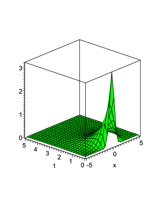
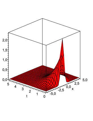
Figure 1: Surfaces representing the $u$ (green) and $v$ (red) components of solution (22) of the DHT system (7) with the parameters $d=1,\ S=3,\ R=1.5,\ t_{0}=0.1.$

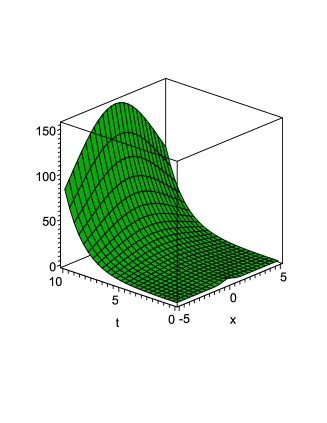
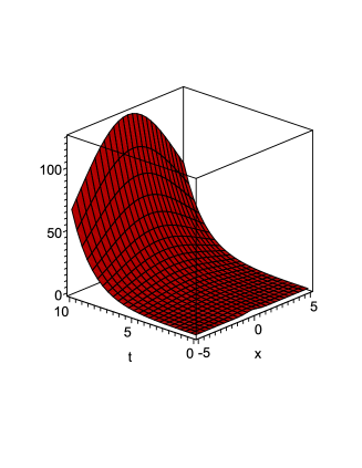
Figure 2: Surfaces representing the $u$ (green) and $v$ (red) components of solution (22) of the DHT system (7) with the parameters $d=1,\ S=3,\ R=0.5,\ t_{0}=0.1.$

In conclusion of this section, we highlight a nontrivial formula for the solution multiplication by using the Lie symmetry of the DHT system (7). In fact, this system with $d=1$ admits four-dimensional Lie algebra (see Case 3 in Table 1), which is nothing else but the Galilei algebra in 1D space $AG(1.1)$ [18]. Thus, applying continuous transformations from the four-parameter Lie group that corresponds to $AG(1.1)$ to a given exact solution $(u_{0}(t,x),v_{0}(t,x))$, one obtains the new solution

$$\begin{array}[]{l}\vskip 6.0pt plus 2.0pt minus 2.0ptu_{new}=Cu_{0}(t+t_{0},x+\varepsilon t+x_{0})\exp\left(\frac{\varepsilon}{2}\left(x+\frac{\varepsilon t}{2}\right)\right),\\ v_{new}=Cv_{0}(t+t_{0},x+\varepsilon t+x_{0})\exp\left(\frac{\varepsilon}{2}\left(x+\frac{\varepsilon t}{2}\right)\right)\end{array}$$ (23)

of system (7) with $d=1$. Here $C,\ t_{0},\ x_{0}$ and $\varepsilon$ are arbitrary parameters, hence (23) represents a four-parameter family of exact solutions. This formula is well-known and valid for any Galilei-invariant system of PDEs (see, e.g., [9, 14]). Although the solution (23) is equivalent to $(u_{0}(t,x),v_{0}(t,x))$ according to the classification of group-invariant solutions of PDEs [30] (see Chapter 3), such type formulae are helpful from the applicability point of view. In particular, the above formula allows us to generate time-dependent solutions from stationary.

4 Conditional symmetries of the DHT model (3)

Let us consider the general form of $Q$-conditional (nonclassical) symmetry operator of system (3)

$$Q=\xi^{0}(t,x,u,v)\partial_{t}+\xi^{1}(t,x,u,v)\partial_{x}+\eta^{1}(t,x,u,v)\partial_{u}+\eta^{2}(t,x,u,v)\partial_{v},\ \left(\xi^{0}\right)^{2}+\left(\xi^{1}\right)^{2}\neq 0,$$ (24)

where $\xi^{i}(t,x,u,v)$ and $\eta^{k}(t,x,u,v)$ are to-be-determined smooth functions. Because the DHT system (3) is a system of evolution equations, the problem of constructing its $Q$-conditional symmetry operators of the form (24) depends on the value of the function $\xi^{0}$ and one needs to consider two essentially different cases :

1. $\xi^{0}\neq 0\Rightarrow\xi^{0}=1.$

2. $\xi^{0}=0,\ \xi^{1}\neq 0.$

Typically, the first case is under study and it is widely thought that the most interesting conditional symmetries are those with $\xi^{0}\neq 0$. The algorithm for finding $Q$-conditional symmetries is well-known and one is based the following criterion (see, e.g., Chapter 5 in [5]).

Definition 1

Operator (24) is called the $Q$-conditional symmetry for the HT system (3) if the following invariance conditions are satisfied:

$$\begin{array}[]{l}\mbox{\raisebox{-6.88889pt}{$\stackrel{{\scriptstyle\displaystyle Q}}{{\scriptstyle 2}}$}}\left(u_{xx}-u_{t}+u\left(1-\frac{R\,v}{u+A}\right)\right)\Big{|}_{{\cal{M}}}=0,\\[8.5359pt] \mbox{\raisebox{-6.88889pt}{$\stackrel{{\scriptstyle\displaystyle Q}}{{\scriptstyle 2}}$}}\left(dv_{xx}-v_{t}+Sv\left(1-\frac{v}{u}\right)\right)\Big{|}_{{\cal{M}}}=0,\end{array}$$

where the manifold

$$\begin{array}[]{l}{\cal{M}}=\Big{\{}S_{1}=0,S_{2}=0,Q(u)=0,Q(v)=0,\vskip 6.0pt plus 2.0pt minus 2.0pt\\ \frac{\partial}{\partial t}\,Q(u)=0,\frac{\partial}{\partial x}\,Q(u)=0,\frac{\partial}{\partial t}\,Q(v)=0,\frac{\partial}{\partial x}\,Q(v)=0\Big{\}},\end{array}$$

while

$$\begin{array}[]{l}S_{1}\equiv\ u_{xx}-u_{t}+u\left(1-\frac{R\,v}{u+A}\right),\\ S_{2}\equiv\ dv_{xx}-v_{t}+Sv\left(1-\frac{v}{u}\right).\end{array}$$

Hereafter we use the notations

$$\begin{array}[]{l}Q(u)=\xi^{0}u_{t}+\xi^{1}u_{x}-\eta^{1},\ Q(v)=\xi^{0}v_{t}+\xi^{1}v_{x}-\eta^{2},\vskip 6.0pt plus 2.0pt minus 2.0pt\\ \mbox{\raisebox{-7.3194pt}{$\stackrel{{\scriptstyle\displaystyle Q}}{{\scriptstyle 2}}$}}=Q+\rho^{1}_{t}\partial_{u_{t}}+\rho^{1}_{x}\partial_{u_{x}}+\rho^{2}_{t}\partial_{v_{t}}+\rho^{2}_{x}\partial_{v_{x}}+\\ \hskip 56.9055pt\sigma^{1}_{tt}\partial_{u_{tt}}+\sigma^{1}_{tx}\partial_{u_{tx}}+\sigma^{1}_{xx}\partial_{u_{xx}}+\sigma^{2}_{tt}\partial_{v_{tt}}+\sigma^{2}_{tx}\partial_{v_{tx}}+\sigma^{2}_{xx}\partial_{v_{xx}},\end{array}$$

where the coefficients $\rho$ and $\sigma$ with relevant subscripts are expressed via the functions $\xi^{i}$ and $\eta^{k}$ by the well-known formulae. As it is shown in [11], the manifold ${\cal{M}}$ can be replaced by

$${\cal{M^{*}}}=\left\{S_{1}=0,S_{2}=0,Q(u)=0,Q(v)=0,\frac{\partial}{\partial t}\,Q(u)=0,Q(v)=0\right\}$$

in the case of evolution systems of PDEs. It turns out that application of the above definition for finding $Q$-conditional symmetries leads to rather trivial results provided $\xi^{0}\neq 0$.

Theorem 2

The DHT system (3) admits only such $Q$-conditional operators of the form (24) with $\xi^{0}\neq 0$, which are equivalent either to the Lie symmetry operators presented in Table 1 or to their linear combinations.

In the case $\xi^{0}=0$, operator (24) takes the form

$$Q=\xi^{1}(t,x,u,v)\partial_{x}+\eta^{1}(t,x,u,v)\partial_{u}+\eta^{2}(t,x,u,v)\partial_{v},\ \xi\neq 0.$$ (25)

It is well-known that the task of constructing the $Q$-conditional symmetries with $\xi^{0}=0$ is much more complicated. In fact, the so-called determining equations (DEs) obtained by applying Definition 1 are so complicated that can be solved only under additional restrictions. It is generally accepted that constructing of a general solution of DEs for a given nonlinear system is equivalent to solving of the system in question (in the case of scalar evolution equations this was shown in [38]). Very recently, it was noted the case $\xi^{0}=0$ can be completely examined using the notion of $Q$-conditional symmetry of the first type [12]. Although this notion was introduced in 2010 [10], its successful applications were realized only in the case $\xi^{0}\neq 0$ (see [11] and references therein). In the case $\xi^{0}=0$, the invariance criteria for $Q$-conditional symmetry of the first type can be formulated as follows.

Definition 2

Operator (25) is called the $Q$-conditional symmetry of the first type for the DHT system (3) if the following invariance conditions are satisfied :

$$\begin{array}[]{l}\mbox{\raisebox{-6.88889pt}{$\stackrel{{\scriptstyle\displaystyle Q}}{{\scriptstyle 2}}$}}\,(S_{1})\Big{|}_{{\cal{M}}_{1}}=0,\\[8.5359pt] \mbox{\raisebox{-6.88889pt}{$\stackrel{{\scriptstyle\displaystyle Q}}{{\scriptstyle 2}}$}}\,(S_{2})\Big{|}_{{\cal{M}}_{1}}=0,\end{array}$$ (26)

where the manifold ${\cal{M}}_{1}$ is either ${\cal{M}}_{1}^{u}=\{S_{1}=0,S_{2}=0,Q(u)=0,\frac{\partial}{\partial t}\,Q(u)=0,\frac{\partial}{\partial x}\,Q(u)=0\}$ or ${\cal{M}}_{1}^{v}=\{S_{1}=0,S_{2}=0,Q(v)=0,\frac{\partial}{\partial t}\,Q(v)=0,\frac{\partial}{\partial x}\,Q(v)=0\}$.

It can be noted that formulae (26) have the same structure at those in Definition 1, however, the manifolds ${\cal{M}}_{1}^{u}$ and ${\cal{M}}_{1}^{v}$ do not coincide with ${\cal{M}}$. It should be stressed that each $Q$-conditional symmetry of the first type is automatically a $Q$-conditional (nonclassical) symmetry but not wise versa [10].

Since system (3) does not possess the symmetric structure we should apply Definition 2 twice, using both manifolds ${\cal{M}}_{1}^{u}$ and ${\cal{M}}_{1}^{v}$. As a result, the following theorem can be formulated.

Theorem 3

The DHT system (3) is invariant under a $Q$-conditional symmetry of the first type (25) if and only if the system and the corresponding symmetry operator possess the forms listed below.

Case I. $d\neq 1$ :

$$\begin{array}[]{l}u_{t}=u_{xx}+u-Sv,\vskip 6.0pt plus 2.0pt minus 2.0pt\\ v_{t}=dv_{xx}+Sv\left(1-\frac{v}{u}\right),\end{array}$$ (27)

$$Q^{u}_{1}=\partial_{x}+f(t)u\partial_{u}+\left(f(t)v-\frac{f^{\prime}(t)}{S}\,u\right)\partial_{v},$$

where the smooth function f(t) is the solution of the nonlinear ODE

$$f^{\prime\prime}+(1-d)f^{2}f^{\prime}+\left(1-S\right)f^{\prime}=0,$$ (28)

which can be presented in an implicit form

$$\int\frac{1}{\frac{d-1}{3}f^{3}+(S-1)f+C_{1}}df=t+C_{2}.$$ (29)

Case II. $d=1$ :

$$\begin{array}[]{l}u_{t}=u_{xx}+u-Sv,\vskip 6.0pt plus 2.0pt minus 2.0pt\\ v_{t}=v_{xx}+Sv\left(1-\frac{v}{u}\right),\end{array}$$ (30)

$$Q^{u}_{2}=2g(t)\partial_{x}+\left(2h(t)-g^{\prime}(t)x\right)u\partial_{u}+\left(\left(2h(t)-g^{\prime}(t)x\right)v-\frac{\left(2h^{\prime}(t)-g^{\prime\prime}(t)x\right)}{S}\,u\right)\partial_{v},$$

where the smooth functions g(t) and h(t) are the solution of the nonlinear ODE system

$$\begin{array}[]{l}hg^{\prime\prime}+g\left(h^{\prime\prime}+\left(1-S\right)h^{\prime}\right)=0,\vskip 6.0pt plus 2.0pt minus 2.0pt\\ gg^{\prime\prime}=Ce^{(S-1)t}.\end{array}$$ (31)

Remark 1

In Teorem 3, the upper index $u$ means that the relevant $Q$-conditional symmetry operator satisfy Definition 2 with the manifold ${\cal{M}}_{1}^{u}$. Application of Definition 2 with the manifold ${\cal{M}}_{1}^{v}$ leads only to Lie symmetries.

Proof of Theorem 3 consists of the same steps as those presented in detail in [12] for the diffusive Lotka–Volterra system. Thus, the relevant analysis and calculations are omitted here.

Remark 2

We were unable to construct the general solution of the nonlinear ODE system (31). However, the nontrivial particular exact solution

$$g(t)=C_{1}e^{\frac{S-1}{2}\,t},\quad h(t)=\left(C_{2}+C_{3}t\right)e^{\frac{S-1}{2}\,t},\ S\neq 1$$ (32)

was identified.

Remark 3

Theorem 3 gives an exhaustive description of $Q$-conditional symmetries of the first type of the DHT system (3). However, one does not present all possible $Q$-conditional (nonclassical) symmetries because $Q$-conditional symmetries of the first type form only a subset of nonclassical symmetries (see [10] for details).

In conclusion of this section, it should be pointed out that the $Q$-conditional symmetries obtained do not coincide with the Lie symmetries presented in Table 1. In fact, the operator $Q^{u}_{1}$ involves a nonconstant function $f(t)$, so that one differs from the Lie symmetries listed in Cases 1 and 2 of Table 1.

The operator $Q^{u}_{2}$ does not coincide with the Lie symmetries listed in Cases 4 and 5 of Table 1 provided $g^{\prime\prime}\neq 0$. If $g(t)$ is a linear function then $h^{\prime\prime}+\left(1-S\right)h^{\prime}=0$. Thus, the operator $Q^{u}_{2}$ takes the forms

$$\alpha_{1}P_{x}+\alpha_{2}\,I+\alpha_{3}\,G+\alpha_{4}\,{\cal{Q}}$$

and

$$\alpha_{1}P_{x}+\alpha_{2}\,I+\alpha_{3}\,G+\alpha_{4}\,Y$$

in the cases $S\neq 1$ and $S=1$, respectively.

5 Non-Lie exact solutions of the DHT model

Here our aim is to construct exact solutions of the DHT systems (27) and (30) using the conditional symmetries obtained in Section 4, examine their properties and suggest a possible interpretation. We note that the case $S=1$ is not examined because the linear terms $u$ and $v$ are removable in this case (see (5)), so that the real-world applicability of the system obtained are questionable.

Let us consider Case I of Theorem 3. To find exact solutions of the DHT system (27) using the operator $Q^{u}_{1}$, we apply the standard procedure. Firstly, the invariant surface conditions

$$Q^{u}_{1}(u)=0,\ Q^{u}_{1}(v)=0,$$

i.e.

$$u_{x}=f(t)u,\quad v_{x}=f(t)v-\frac{f^{\prime}(t)}{S}\,u$$ (33)

should be solved. (33) is the system of the linear first-order PDEs involving the function $f(t)$ in an implicit form (see (29)). Solving this system, one obtains the ansatz

$$\begin{array}[]{l}u(t,x)=\varphi(t)e^{xf(t)},\vskip 6.0pt plus 2.0pt minus 2.0pt\\ v(t,x)=\psi(t)e^{xf(t)}-\frac{xf^{\prime}}{S}\,\varphi(t)e^{xf(t)},\end{array}$$ (34)

where $\varphi$ and $\psi$ are new unknown functions. Substituting ansatz (34) into (27) and taking into account (28), one derives the reduced system of ODEs

$$\begin{array}[]{l}\varphi^{\prime}=\left(1+f^{2}\right)\varphi-S\psi,\vskip 6.0pt plus 2.0pt minus 2.0pt\\ \psi^{\prime}=\left(S+df^{2}\right)\psi-\frac{S}{\varphi}\psi^{2}-\frac{2dff^{\prime}}{S}\varphi.\end{array}$$ (35)

System (35) can be rewritten in the form

$$\begin{array}[]{l}\psi=\frac{\varphi^{\prime}-\left(1+f^{2}\right)\varphi}{S},\vskip 6.0pt plus 2.0pt minus 2.0pt\\ \varphi^{\prime\prime}-\frac{{\varphi^{\prime}}^{2}}{\varphi}+K_{1}(t)\varphi^{\prime}+K_{0}(t)\varphi=0,\end{array}$$ (36)

where

$$K_{1}(t)=1-S+(1-d)f^{2},\ K_{0}(t)=S-1+(d+S-2)f^{2}+(d-1)f^{4}-2(d+1)ff^{\prime}.$$ (37)

By applying substitution (13), the second equation of system (36) reduces to the linear ODE

$$\chi^{\prime}+K_{1}\chi+K_{0}=0.$$ (38)

Thus, solving the equations (38) and (13) and taking into account formulae (36) and (37), one obtains the functions $\varphi$ and $\psi$. Finally, exact solutions of the DHT system (27) in the form (34) can be easily written down. From the applicability point of view, the solutions obtained are not convenient because they involve the function $f(t)$ in an implicit form.

Now we present an example constructing the exact solution on the DHT system (27) in an explicit form. Firstly, one needs to identify the function $f$ in the explicit form. Obviously, it occurs if one sets $C_{1}=0$ in (29). Note that an arbitrary constant $C_{2}$ can be taken $C_{2}=0$ as well without loosing a generality. In this special case

$$f=\pm\sqrt{\frac{S-1}{1+\frac{1-d}{3}\,e^{2\left(S-1\right)t}}}\,e^{\left(S-1\right)t}.$$ (39)

Thus, the coefficients $K_{0}$ and $K_{1}$ in (38) have the forms

$$\begin{array}[]{l}K_{1}=\frac{(1-S)\,\left(3+2(d-1)e^{2\left(S-1\right)t}\right)}{3+(1-d)e^{2\left(S-1\right)t}},\vskip 6.0pt plus 2.0pt minus 2.0pt\\ K_{0}=\frac{1-S}{\left(3+(1-d)e^{2\left(S-1\right)t}\right)^{2}}\,\left(b_{2}e^{4\left(S-1\right)t}+b_{1}e^{2\left(S-1\right)t}-9\right),\end{array}$$ (40)

where

$$b_{1}=3(3S+6dS-7d-2),\quad b_{2}=2(d-1)(2+d-3S).$$

After straightforward calculations, we obtain the following functions $\varphi$ and $\psi$ :

$$\begin{array}[]{l}\varphi(t)=\exp\left(G(t)+t\right)\left(3+(1-d)e^{2\left(S-1\right)t}\right)^{\frac{3(2d-1)}{2(d-1)}},\vskip 6.0pt plus 2.0pt minus 2.0pt\\ \psi(t)=\frac{3(1-S)\,G(t)}{S\left(3+(1-d)\,e^{2\left(S-1\right)t}\right)}\,\varphi(t),\end{array}$$ (41)

where

$$G(t)=\left\{\begin{array}[]{l}\frac{e^{\left(S-1\right)t}}{\sqrt{3+(1-d)e^{2\left(S-1\right)t}}}\left[C+\frac{6d}{\sqrt{1-d}}arcsinh\left(\frac{\sqrt{1-d}}{\sqrt{3}}e^{\left(S-1\right)t}\right)\right],\quad d<1,\\ \frac{e^{\left(S-1\right)t}}{\sqrt{3+(1-d)e^{2\left(S-1\right)t}}}\left[C+\frac{6d}{\sqrt{d-1}}arcsin\left(\frac{\sqrt{d-1}}{\sqrt{3}}e^{\left(S-1\right)t}\right)\right],\quad d>1.\end{array}\right.$$

Formulae (39) and (41) lead to the exact solution

$$\begin{array}[]{l}u(t,x)=\Big{(}3+(1-d)e^{2\left(S-1\right)t}\Big{)}^{\frac{3(2d-1)}{2(d-1)}}\exp\left(G(t)+t\pm\sqrt{\frac{3(S-1)}{3+(1-d)e^{2\left(S-1\right)t}}}\,e^{\left(S-1\right)t}\,x\right),\vskip 6.0pt plus 2.0pt minus 2.0pt\\ v(t,x)=\left[\frac{3(1-S)}{S}\Big{(}3+(1-d)\,e^{2\left(S-1\right)t}\Big{)}^{-1}\,G(t)\mp\sqrt[3]{\frac{3(S-1)}{3+(1-d)e^{2\left(S-1\right)t}}}e^{(S-1)t}\,x\right]\,u(t,x)\end{array}$$

of the DHT system (27).

Case II of Theorem 3. Solving the first-order PDEs

$$Q^{u}_{2}(u)=0,\ Q^{u}_{2}(v)=0,$$

one obtains the ansatz

$$\begin{array}[]{l}u(t,x)=\varphi(t)\exp\left(\frac{h}{g}\,x-\frac{g^{\prime}}{4g}\,x^{2}\right),\vskip 6.0pt plus 2.0pt minus 2.0pt\\ v(t,x)=\left(\psi(t)-\frac{\varphi(t)\,x}{4Sg}\left(4h^{\prime}-g^{\prime\prime}x\right)\right)\exp\left(\frac{h}{g}\,x-\frac{g^{\prime}}{4g}\,x^{2}\right),\end{array}$$ (42)

where $\varphi$ and $\psi$ are functions to be found, while the functions $g$ and $h$ satisfy system (31). Substituting ansatz (42) into the DHT system (30), we arrive at the reduced system of ODEs

$$\begin{array}[]{l}\varphi^{\prime}=\left(1+\frac{h^{2}}{g^{2}}-\frac{g^{\prime}}{2g}\right)\varphi-S\psi,\vskip 6.0pt plus 2.0pt minus 2.0pt\\ \psi^{\prime}=\left(S+\frac{h^{2}}{g^{2}}-\frac{g^{\prime}}{2g}\right)\psi-\frac{S}{\varphi}\psi^{2}+\frac{gg^{\prime\prime}-4hh^{\prime}}{2Sg^{2}}\varphi.\end{array}$$ (43)

Similarly to the ODE system (36), system (43) can be easily solved. Indeed, using the first equation of system (43), we immediately obtain

$$\psi=\frac{1}{S}\left[-\varphi^{\prime}+\left(1+\frac{h^{2}}{g^{2}}-\frac{g^{\prime}}{2g}\right)\varphi\right].$$

Substituting the function $\psi$ and its first-order derivative into the second equation of (43) and applying the substitution (13), we obtain the linear ODE

$$\chi^{\prime}+(1-S)\chi+K(t)=0,$$ (44)

where

$$K(t)=S-1+\frac{1}{2g^{2}}\Big{(}2g^{2}g^{\prime\prime}-g{g^{\prime}}^{2}+(4h^{2}+g^{2}-Sg^{2})g^{\prime}+2h(Sh-h-4h^{\prime})g\Big{)}.$$

Thus, having the correctly-specified functions $g$ and $h$, ODE (44) can be easily solved and the functions $\varphi$ and $\psi$ constructed. To obtain exact solutions of the DHT system (30) in an explicit form, we use the functions $g$ and $h$ from (32). Thus,

$$K(t)=-\frac{S^{2}-10S+9}{8}-\frac{4C_{3}(C_{2}+C_{3}t)}{C_{1}^{2}}.$$

Integrating (44) and (13) and renaming $C_{2}\rightarrow C_{1}\left(C_{2}-2C_{3}\right),\ C_{3}\rightarrow\left(S-1\right)C_{1}C_{3}$, we arrive at the solution

$$\begin{array}[]{l}\varphi(t)=\exp\Big{[}\frac{9-S}{8}\,t-4C_{3}(C_{2}-C_{3})\,t+2C_{3}^{2}\left(1-S\right)\,t^{2}+Ce^{(S-1)t}\Big{]},\vskip 6.0pt plus 2.0pt minus 2.0pt\\ \psi(t)=\frac{1}{S}\Big{[}\frac{1-S}{8}+\big{(}C_{2}+C_{3}(S-1)t\big{)}^{2}+(1-S)Ce^{(S-1)t}\Big{]}\varphi(t)\end{array}$$ (45)

of the ODE system (43).

Finally, substituting (45) into ansatz (42) and taking into account (32), we obtain the three-parameter family of exact solutions of system (30)

$$\begin{array}[]{l}u(t,x)=\exp\Big{[}\left(\frac{9-S}{8}-4C_{3}^{2}\right)\,t+(2C_{3}-C_{2})(4C_{3}t-x)-\frac{1}{8}(S-1)(4C_{3}t-x)^{2}+Ce^{(S-1)t}\Big{]},\\ \vskip 6.0pt plus 2.0pt minus 2.0pt\\ v(t,x)=\frac{1}{16S}\Big{[}\big{(}4C_{2}+(S-1)(4C_{3}t-x)\big{)}^{2}-2(S-1)\big{(}1+8Ce^{(S-1)t}\big{)}\Big{]}u(t,x),\end{array}$$ (46)

where $C,\,C_{2}$ and $C_{3}$ are arbitrary parameters.

Remark 4

Since the DHT system (30) admits the Galilei operator $G$, the exact solution (46) can be presented in the simpler form. Indeed,using formula (23), solution (46) can be simplified to the form

$$\begin{array}[]{l}u(t,x)=\exp\Big{[}\frac{9-S}{8}\,t+C_{2}x-\frac{S-1}{8}x^{2}+Ce^{(S-1)t}\Big{]},\\ \vskip 6.0pt plus 2.0pt minus 2.0pt\\ v(t,x)=\frac{1}{16S}\Big{[}\big{(}4C_{2}-(S-1)x\big{)}^{2}-2(S-1)\big{(}1+8Ce^{(S-1)t}\big{)}\Big{]}u(t,x)\end{array}$$

(here the upper index $*$ is omitted). The relevant Galilei transformation is

$$x^{*}=x-4C_{3}t,\ u^{*}=\exp\left(2C_{3}x-4C_{3}^{2}t\right)u,\ v^{*}=\exp\left(2C_{3}x-4C_{3}^{2}t\right)v.$$

To present some biological interpretation, one may consider a specific solution by setting $C_{2}=C_{3}=0$ in (46). In this case, the exact solution is as follows

$$\begin{array}[]{l}u(t,x)=\exp\left(\frac{9-S}{8}\,t+Ce^{(S-1)t}-\frac{S-1}{8}\,x^{2}\right),\vskip 6.0pt plus 2.0pt minus 2.0pt\\ v(t,x)=\frac{S-1}{16S}\left(-2-16Ce^{(S-1)t}+(S-1)x^{2}\right)u(t,x).\end{array}$$ (47)

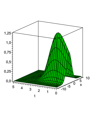
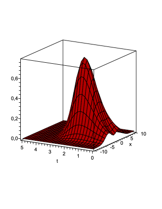
Figure 3: Surfaces representing the $u$ (green) and $v$ (red) components of the exact solution (47) of the DHT system (30). The parameters $S=2,\ C=-0.25$.

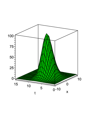
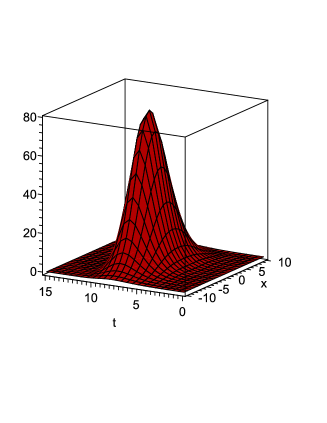
Figure 4: Surfaces representing the $u$ (green) and $v$ (red) components of the exact solution (47) of the DHT system (30). The parameters $S=1.4,\ C=-0.125$.

The components of solution (47) are bounded and positive in the domain

$$\Omega=\left\{(t,x)\in(0,+\infty)\times(-\infty,+\infty)\right\}$$

provided the coefficient restrictions $C\leq-\frac{1}{8},\ S>1$ hold. Moreover, solution (47) satisfies the zero Neumann conditions at infinity

$$u_{x}(t,-\infty)=u_{x}(t,+\infty)=v_{x}(t,-\infty)=v_{x}(t,+\infty)=0$$

in the domain $\Omega$. One also easily checks that the asymptotic behaviour

$$(u,\,v)\rightarrow(0,\,0)\quad\mbox{as}\quad t\rightarrow+\infty$$

takes place, which predicts a total extinction of the both species $u$ and $v$. An example of solution (47) is presented in Fig. 3 (Fig. 4 highlights the same scenario for preys and predators but with the initial profiles approaching zero densities). One can note that the zero-flux conditions are satisfied with a sufficient exactness at any bounded space interval $[a,\ b]$ with $|a|>10,\ |b|>10$. It can be regarded as a habit of the both species to concentrate themselves in a compact area. For example, it may happen if the compact area is a forest with large amount of food for preys. To the best of our knowledge, such type solutions are unknown for the diffusive Lotka–Volterra system modelling the prey-predator interaction.

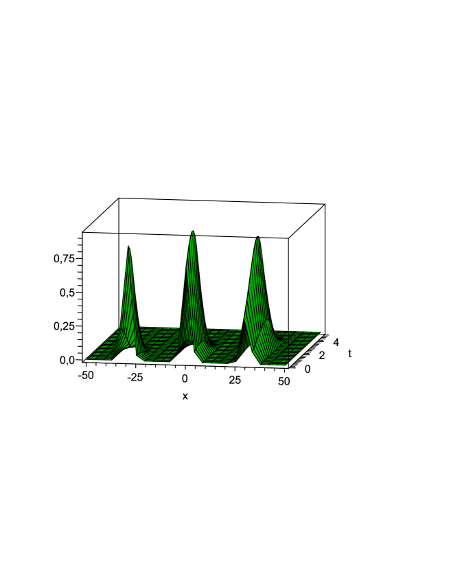
Figure 5: Surface representing the component $U$ of the approximate solution (46) of the DHT systems (30). The parameters $S=2,\ C=-0.35$, $x_{0}=-30,\ x_{1}=0,\ x_{2}=30,\ t_{0}=-1,\ t_{1}=0,\ t_{2}=1.$

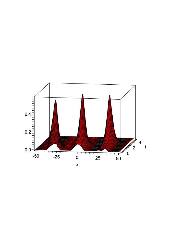
Figure 6: Surface representing the component $V$ of the approximate solution (46) of the DHT systems (30). The parameters $S=2,\ C=-0.35$, $x_{0}=-30,\ x_{1}=0,\ x_{2}=30,\ t_{0}=-1,\ t_{1}=0,\ t_{2}=1.$

Now we present an observation, which is highly unusual for nonlinear PDEs, for which the well-known principle of linear superposition of solutions is not valid. Because the DHT model admits the time and space translations, the exact solution (47) can be rewritten in the form

$$\begin{array}[]{l}u(t,x)=\exp\Big{[}\frac{9-S}{8}\,(t+t_{0})+C\exp\big{(}(S-1)(t+t_{0})\big{)}-\frac{S-1}{8}\,(x+x_{0})^{2}\Big{]},\vskip 6.0pt plus 2.0pt minus 2.0pt\\ v(t,x)=\frac{S-1}{16S}\Big{[}-2-16C\exp\big{(}(S-1)(t+t_{0})\big{)}+(S-1)(x+x_{0})^{2}\Big{]}u(t,x),\end{array}$$ (48)

where $t_{0}$ and $x_{0}$ are arbitrary parameters. Similarly to (47), each exact solution (48) with a fixed pair $(t_{0},x_{0})$ is bounded and positive in the domain $\Omega$ provided the restrictions $C\leq C_{0}=-\frac{1}{8}e^{(1-S)t_{0}},\ S>1$ hold. On the other hand, the solution decays very sharply if $|x+x_{0}|\to\infty$, because both components contain multiplier $\exp\left(-\frac{S-1}{8}\,(x+x_{0})^{2}\right)$. For example, one notes from Fig. 3 that both components $u$ and $v$ of solution (47) practically vanish if $|x|>10$. So, taking solution (48), say with $t_{0}=0$ and $x_{0}=30$, one observes that this solution vanishes with a high exactness beyond the interval $x\in[-40,-20]$. Now we conclude that the expressions

$$u(t,x)+u(t+t_{0},x+x_{0}),\quad v(t,x)+v(t+t_{0},x+x_{0}),$$

where the functions $u$ and $v$ are the exact solutions of the form (47) and (48), produce an approximate solution of the DHT systems (30) provided $|x_{0}|$ is sufficiently large. Moreover, a further generalization of the form

$$\begin{array}[]{l}U(t,x)=u(t+t_{0},x+x_{0})+u(t+t_{1},x+x_{1})+\dots+u(t+t_{m},x+x_{m}),\\ V(t,x)=v(t+t_{0},x+x_{0})+v(t+t_{1},x+x_{1})+\dots+v(t+t_{m},x+x_{m})\end{array}$$ (49)

presents another approximate solution of the DHT systems (30) provided the differences $|x_{i}-x_{j}|,\ (0\leq i<j\leq m)$ are sufficiently large. An example of the approximate solution (49) is presented in Fig. 5–Fig. 6.

6 Conclusions

In this work, the DHT prey-predator model (under the assumption of the Malthusian growth low for preys) is investigated by means of Lie and $Q$-conditional (nonclassical) symmetry methods. Applying the classical Lie method, all Lie symmetries of the model in question were found (see Theorem 1) and it was shown that these symmetries coincide with those, which follow from the earlier works although [14, 15]. The results presented in Theorems 2 and 3 are new and highly nontrivial. In fact, $Q$-conditional symmetries of the DHT system (3) are found for the first time. It is also proved that this system admits only those $Q$-conditional symmetries with $\xi^{0}\not=0$ (see (24)), which are equivalent to the Lie symmetry operators listed in Theorem 1. However, applying the algorithm based on the recently introduced Definition 2, we found new $Q$-conditional symmetries in the ‘no-go case’ ($\xi^{0}=0$ in (24)).

Both Lie and $Q$-conditional symmetries are applied for construction of exact solutions via reduction of the DHT system (3) to ODE systems and solving the latter. The most interesting (from the applicability point of view) Cases 1 and 3 of Table 1 has been examined. As a result, several families of exact solutions are derived. Interestingly, the exact solutions derived via $Q$-conditional symmetries (see formulae (47)–(48)) are non-Lie solutions, i.e. they cannot be found using the Lie ansätze listed in Table 2. We remind the reader that a given $Q$-conditional symmetry, generally speaking, does not lead to non-Lie solutions (see the relevant discussion and examples in Chapter 4 [16]).

Because some solutions (see (22) and (47)) possess remarkable properties, in particular boundedness and nonnegativity, a possible biological interpretation is suggested and the relevant plots are presented.

Finally, we presented a formula for generation of approximate solutions of the DHT system (3). The formula allows us to construct such approximate solutions, which consist of several ‘peaks’ (see Fig. 5 and 6). Interestingly that the approximate solutions (49) have a very similar structure to the numerical solutions derived in [28] (see Fig. 3 therein) for the activator-inhibitor model

$$\begin{array}[]{l}u_{t}=d_{1}u_{xx}-a_{1}u+b_{1}v^{2},\vskip 6.0pt plus 2.0pt minus 2.0pt\\ v_{t}=d_{2}v_{xx}-a_{2}v+b_{2}\frac{v^{2}}{u}\end{array}$$ (50)

(here all parameters are positive constants). System (50) was developed in the seminal work [19] and is motivated by biological experiments on hydra. One easily notes that the above system coincides with the DHT sytem (7) if one replace the quadratic term $b_{1}v^{2}$ by linear and takes the opposite signs in reactive terms.

Acknowledgments. R.Ch. acknowledges that this research was funded by the British Academy’s Researchers at Risk Fellowships Programme. The authors are grateful to Reviewer 1 for fruitful comments that can be used in future studies of the DHT system.

References

[1] Arancibia-Ibarra, C., Bode, M., Flores, J.,
Pettet, G., Van Heijster, P.: Turing patterns in a diffusive
Holling–Tanner predator-prey model with an alternative food source
for the predator. Comm. Nonlinear Sci. Numer. Simulat. 99,
105802 (2021)
[2] Aris, R.:
The Mathematical Theory of Diffusion and
Reaction in Permeable Catalysts: the Theory of
the Steady State. Clarendon Press, Oxford (1975)
[3] Arrigo, D.J.: Symmetry Analysis of Differential Equations: an
Introduction. John Wiley & Sons, Hoboken (2015)
[4] Aziz-Alaoui, M.A., Daher Okiye, M., Moussaoui, A.: Permanence
and extinction of a diffusive predator-prey model with Robin
boundary conditions. Acta Biotheoretica 66, 367–378 (2018)
[5] Bluman, G.W., Cheviakov, A.F., Anco, S.C.: Applications of Symmetry
Methods to Partial Differential Equations. Springer, New York (2010)
[6] Britton, N.F.: Essential Mathematical
Biology. Springer, Berlin (2003)
[7] Broadbridge, P., Cherniha, R.M., Goard,
J.M.: Exact nonclassical symmetry solutions of Lotka–Volterra-type
population systems. Euro. J. Appl. Math. 1–19, (2022)
[8] Chen, S., Shi, J.: Global stability in a diffusive
Holling–Tanner predator-prey model. Appl. Math. Lett. 25,
614–618 (2012)
[9] Cherniha, R.M.: On exact solutions of a nonlinear
diffusion-type system.
In: Symmetry analysis and exact solutions of
equations of mathematical physics, Kyiv, Inst. Math. Ukrainian
Acad. Sci., 49–53 (1988)
[10] Cherniha, R.: Conditional symmetries
for systems of PDEs: new definition and their application for
reaction-diffusion systems. J. Phys. A: Math.
Theor. 43, 405207 (2010)
[11] Cherniha, R., Davydovych, V.:
Nonlinear Reaction-Diffusion Systems — Conditional Symmetry, Exact
Solutions and their Applications in Biology. Lecture Notes in
Mathematics, vol. 2196. Springer, Cham (2017)
[12] Cherniha, R., Davydovych,
V.: New conditional symmetries and exact solutions of the diffusive
two-component Lotka–Volterra system. Mathematics 9, 1984
(2021)
[13] Cherniha, R., Davydovych, V.: A hunter–gatherer-farmer population model: new
conditional symmetries and exact solutions with biological
interpretation. Acta Appl. Math. 182, 4 (2022)
[14] Cherniha, R., King, J.R.:
Lie symmetries of nonlinear multidimensional
reaction-diffusion systems: I. J. Phys A: Math. Gen. 33,
267–282 (2000)
[15] Cherniha, R., King, J.R.:
Lie symmetries of nonlinear multidimensional
reaction-diffusion systems: II. J. Phys A: Math. Gen. 36,
405–425 (2003)
[16] Cherniha, R., Serov, M., Pliukhin, O.:
Nonlinear Reaction-Diffusion-Convection Equations: Lie and
Conditional Symmetry, Exact Solutions and their Applications.
Chapman and Hall/CRC, New York (2018)
[17] Fife, P.: Mathematical Aspects of Reacting and Diffusing Systems.
Springer, New York (1975)
[18] Fushchych, W.I., Cherniha, R.M.: Galilei-invariant systems of nonlinear systems of
evolution equations. J. Phys. A: Math. Gen. 28, 5569–5579
(1995)
[19] Gierer, A., Meinhardt, H.: A theory of biological pattern formation. Kybernetik
12, 30–39 (1972)
[20] Hanski, I., Hansson, L., Henttonen, H.: Specialist
predators, generalist predators, and the microtine rodent cycle. J.
Anim. Ecol. 60, 353–367 (1991)
[21] Hanski, I., Turchin, P., Korpimäki, E., Henttonen,
H.: Population oscillations of boreal rodents: regulation by
mustelid predators leads to chaos. Nature 364, 232–235
(1993)
[22] Kuang, Y., Nagy, J.D., Eikenberry, S.E.: Introduction to Mathematical Oncology.
CRC Press, Boca Raton (2016)
[23] Lina, J.i.:
The method of linear determining equations to evolution
system and application for reaction-diffusion system with power diffusivities.
Symmetry 8, 157 (2016)
[24] Lotka, A.J.:
Undamped oscillations derived from the law of mass action. J. Am.
Chem. Soc. 42, 1595–1599 (1920)
[25] Murray, J.D.: Mathematical Biology. Springer, Berlin
(1989)
[26] Murray, J.D.:
Mathematical Biology I. Springer, Berlin (2002)
[27] Murray, J.D.:
Mathematical Biology II. VSpringer, Berlin (2003)
[28] Ni, W.M.: Diffusion, cross-diffusion,
and their spike-layer steady states. Not. AMS 45, 9–18
(1998)
[29] Okubo, A., Levin, S.A.: Diffusion and Ecological Problems.
Modern Perspectives, 2nd edn. Springer, Berlin (2001)
[30] Olver, P.:
Applications of Lie Groups to Differential Equations. 2nd edn.
Springer, Berlin (1993)
[31] Patera, J., Winternitz, P.: Subalgebras of real three- and
four-dimensional Lie algebras. J. Math. Phys. 18,
1449–1455 (1977)
[32] Qi, Y., Zhu, Y.: The study of global stability of
a diffusive Holling–Tanner predator-prey model. Appl. Math. Lett. 57,
132–138 (2016)
[33] Tanner, J.T. The stability and the intrinsic growth rates
of prey and predator populations. Ecology 56, 855–867
(1975)
[34] Torrisi, M., Tracina, R.: Lie
symmetries and solutions of reaction-diffusion systems arising in
biomathematics. Symmetry 13, 1530 (2021)
[35] Torrisi, M., Tracina, R.:
Symmetries and solutions for a class of ddvective reaction-diffusion
systems with a special reaction term. Mathematics 11, 160
(2023)
[36] Volterra, V.: Variazioni e fluttuazioni del numero
d‘individui in specie animali conviventi. Mem. Acad. Lincei.
2, 31–113 (1926)
[37] Wollkind, D.J., Collings, J.B., Logan, J.A.:
Metastability in a temperature-dependent model system for
predator-prey mite outbreak interactions on fruit trees. Bull. Math.
Biol. 50, 379–409 (1988)
[38] Zhdanov, R.Z., Lahno, V.I.: Conditional symmetry of a porous
medium equation. Phys. D 122, 178–86 (1998)