We studied numerically the dynamics of colliding rigid bodies in a Newtonian fluid. The finite element method is used to solve the fluid-body interaction and the fluid motion is described in the Arbitrary-Lagrangian-Eulerian framework. To model the interactions between bodies, we consider a repulsive collision-avoidance model, defined by R. Glowinski in [1]. The main emphasis in this work is the generalization of this collision model to multiple rigid bodies of arbitrary shape. Our model first uses a narrow-band fast marching method to detect the set of colliding bodies. Then, collision forces and torques are computed for these bodies via a general expression, which does not depend on their shape. Numerical experiments examining the performance of the narrow-band fast marching method and the parallel execution of the collision algorithm are discussed. We validate our model with literature results and show various applications of colliding bodies in two and three dimensions. In these applications, the bodies either move due to gravity, a flow, or can actuate themselves. Finally, we present a tool to create arbitrary shaped bodies in complex already discretized fluid domains, enabling conforming body-fluid interface and allowing to perform simulations of fluid-body interactions with collision treatment in these realistic environments. All simulations are conducted with the Feel++ open source library.

Keywords: Fluid-structure interaction, rigid body motion, collision simulation, Feel++,
MSC 2010 65M60, 74F10, 76M10, 70E99

Introduction

Fluid flows laden with particles are common in industrial and biological processes, such as fluidization, the cell transport in arteries, or the simulated motion of articulated micro-swimmers in the human body. Due to the particle volume and the confined environments, these processes are characterized by inter-particle interactions. The modeling of these interactions, based on collision detection algorithms, and the computation of lubrication and collision forces, is challenging for arbitrary shaped particles and add further complexity to the coupled fluid-solid interaction problem.

In recent years, various approaches simulating solid-solid or solid-wall interactions have been developed and proposed in the literature. These approaches are based on collision and lubrication forces, added to the system when solving the fluid-solid interactions [2]. When the distance between solid surfaces is small, approximately the mesh size of the computational grid, the fluid placed between the solids is squeezed out and the hydrodynamics are not resolved. The resulting underestimation of the hydrodynamic forces is compensated by a short-range repulsive correction given analytically and called lubrication force. In [3], this lubrication force is defined by a constant expression and in [4] its magnitude is inversely proportional to the distance between the solid surfaces. In some approaches, the lubrication model allows avoiding the direct contact between the solid surfaces [1]. Such contact avoidance schemes are frequently used in literature to simulate the interactions between spherical bodies. In this paper, we will present the generalization of these schemes for complex shaped and articulated bodies. The contact avoidance models often require the adjustment of stiffness parameters, for which the optimal values are not known. Over- or underestimation of these values can falsify the results. To overcome this issue, the authors in [5] solve a minimization problem to determine the minimal force magnitude ensuring a fixed separation distance between the solids at each time step and in [6] the authors introduce the gluey particle method.

A collision force is applied, when the lubrication correction does not avoid the direct contact between the solids. Common collision forces are based on the soft-sphere or hard-sphere approach. When two solids are in direct contact or overlapping, the soft-sphere approach defines the collision force according to the geometrical characteristics of this contact [7]. The approach requires a small time step to resolve the collision process. In contrast, the hard-sphere approach [3] assumes that the collision force is impulsive. During the collision process, the velocities of the interacting solids change instantaneously at the time of contact. The magnitude of the new velocities depends on the pre-collision velocities and some physical parameters.

For large fluid systems, efficient collision detection algorithms are mandatory. These algorithms identify the pairs of solids that are actually interacting, before computing the collision forces only for the respective pairs, which reduces the computational costs. Most collision detection algorithms contain two phases, the broad-phase and the narrow-phase. First, the broad-phase uses spatial partitioning or sorting methods to determine the smallest possible set of neighbouring pairs that are likely to interact. In spatial partitioning, the fluid system is divided into regions and all solids assigned to the same region are considered as neighbours. The data structures employed for spatial partitioning and neighbour detection are lists [8], trees [9], adapted for large number of solids, or hash tables [10], efficient for solids with a wide range of sizes. The spatial sorting methods, as the Sort and Sweep algorithm [11], sort the solids in space to determine overlapping. Then, the narrow-phase detects whether these pairs are actually in contact by computing the distance between the solid surfaces. The distance computation being evident for spherical solids, it is a challenging and often expensive task for complex shaped or articulated bodies. In the literature, multiple analytical methods for specific geometries or general algorithms for arbitrary solid shapes are proposed [2]. Our model uses the fast marching method [12] to track the distance between any pair of arbitrary shaped bodies. Focusing on fluid systems containing up to one hundred solids, the implementation of a broad-phase algorithm is not necessary. However, to avoid the high computational costs associated to the fast marching method, we adapt a narrow-band approach, executable in parallel.

The paper is organized as follows. Section 1 details the coupled problem describing the fluid-solid interaction. The collision model including the collision detection algorithm based on the narrow-band fast marching method and the computation of the contact avoidance lubrication force is presented in section 2. The performance verification and the validation of the model are done in sections 3 and 4. Section 5 shows some applications of the collision model, including simulations of single complex shaped and articulated solids as well as spherical multi-bodies interactions. A summary and conclusions are given in section 6.

1 Rigid body moving in a fluid

This section briefly describes the coupled fluid-rigid body interaction problem. A detailed description is given in [13].

The fluid model

The fluid model considered throughout the paper is incompressible and Newtonian, and the motion of the fluid domain is modelled using the Arbitrary-Lagrangian-Eulerian (ALE) formalism [14]. Let $\mathcal{F}_{t}\subseteq\mathbb{R}^{d},d\in\{2,3\},$ denote the domain occupied by the fluid at time $t$, where $t\in[0,T]$ and $T$ the final time of the simulation. Let $\mathcal{A}_{t}:\mathcal{F}_{0}\to\mathcal{F}_{t}$ be the ALE map mapping the reference fluid domain $\mathcal{F}_{0}$ to the current domain $\mathcal{F}_{t}$, defined as $\mathcal{A}_{t}(X)=\mathcal{A}(t,X)=X+x(t,X)$ with $x(t,X)$ the displacement of the domain. Let $u:\mathcal{F}_{t}\times[0,T]\to\mathbb{R}^{d}$ and $p:\mathcal{F}_{t}\times[0,T]\to\mathbb{R}$ the fluid velocity and the hydrostatic pressure. Let $\rho_{f}$ and $\mu$ be the fluid density and dynamic viscosity, constant for the considered fluid model. Finally, let $\sigma\in\mathcal{M}_{d}(\mathbb{R})$ be the fluid stress tensor and $g\in\mathbb{R}^{d}$ the gravity acceleration. The ALE formulation of the Navier-Stokes equations partially decouples the geometric evolution of the fluid domain from that of the fluid continuum. Due to the change of frame, the ALE time derivative substitutes the Eulerian one $\partial_{t}u$ as $\partial_{t}u=\partial_{t}u|_{\mathcal{A}}-(\partial_{t}x\cdot\nabla)u=\partial_{t}u|_{x}-(u_{\mathcal{A}}\cdot\nabla)u$ in the momentum equation. The first term of the ALE derivative corresponds to the time variation of the fluid velocity as seen in the arbitrary frame, while the second contains the relative velocity between the fluid continuum and the new reference frame. The Navier-Stokes equations in the ALE frame are:

$$\rho_{f}\partial_{t}u|_{\mathcal{A}}+\rho_{f}\Big{(}(u-u_{\mathcal{A}})\cdot\nabla\Big{)}u =-\nabla\cdot\sigma+\rho_{f}g,\qquad \mathcal{F}_{t}$$ in , (1)

$$\nabla\cdot u =0,\qquad \text{in $\mathcal{F}_{t}$}.$$

The rigid body equations

A rigid body moving in a fluid is described by the motion of its center of mass, given by the Newton equation, and the rotation matrix between its local frame and the laboratory frame, defined by the Euler equation. In this paper, the motion of a body is caused by fluid stresses and gravity, contact and lubrication forces that act as external forces $F_{e}$ and torques $T_{e}$. Let $\mathcal{S}\subset\mathbb{R}^{d}$ be the domain occupied by the body, $\rho_{\mathcal{S}}\in\mathbb{R}_{>0}$ its density and $m=\int_{\mathcal{S}}\rho_{\mathcal{S}}$ its mass. Let $U:[0,T]\to\mathbb{R}^{d}$ and $\omega:[0,T]\to\mathbb{R}^{d^{*}}$, where $d^{*}=1$ if $d=2$ or $d^{*}=3$ if $d=3$, be the linear and angular velocity of the rigid body as seen from the laboratory frame. Let $x^{CM}=m^{-1}\int_{\mathcal{S}}\rho_{\mathcal{S}}x$ be its center of mass, $x^{CM}\in\mathbb{R}^{d}$, and $I=\int_{\mathcal{S}}\rho_{\mathcal{S}}(x-x^{CM})\otimes(x-x^{CM})$ its inertia tensor, $I\in S^{d^{*}}_{++}$ positive definite and symmetric. We chose to describe the rotation matrix $R(\theta):\Theta\to SO(d)$ using Euler angles $\theta\in\Theta$, where $\Theta=[-\pi,\pi]$ if $d=2$, or $\Theta=[-\pi,\pi]\times[0,\pi]\times[0,\pi/2]$ if $d=3$. The Newton and Euler equations, describing the dynamics of a three-dimensional rigid body, are:

$$m\frac{d}{dt}U =F_{e}-\int_{\partial\mathcal{S}}-pn+\mu(\nabla u+\nabla u^{T})n,$$ (2)

$$\frac{d}{dt}(RIR^{T}\omega) =T_{e}-\int_{\partial\mathcal{S}}[-pn+\mu(\nabla u+\nabla u^{T})n]\times(x-x^{CM}),$$

where $n$ is the unit outward normal to $\partial\mathcal{S}$ and one has:

$$\frac{d}{dt}\theta_{i} =\omega_{i},\quad\text{for $i\in\{x,y,z\}$},$$

$$R =R_{z}(\theta_{z})R_{y}(\theta_{y})R_{x}(\theta_{x}),$$

where $R(\theta_{i})$ denotes the rotation matrix around axis $i\in\{x,y,z\}$ of angle $\theta_{i}$. If $d=2$, $R(\theta)$ has the form:

$$R(\theta) =\begin{bmatrix}\cos(\theta)&\sin(\theta)\\ -\sin(\theta)&\cos(\theta)\end{bmatrix},$$

while in three dimensions:

$$R_{z}(\theta_{z})=\begin{bmatrix}\cos(\theta_{z})&-\sin(\theta_{z})&0\\ \sin(\theta_{z})&\cos(\theta_{z})&0\\ 0&0&1\end{bmatrix},R_{y}(\theta_{y})=\begin{bmatrix}\cos(\theta_{y})&0&\sin(\theta_{y})\\ 0&1&0\\ -\sin(\theta_{y})&0&\cos(\theta_{y})\end{bmatrix},\\$$

$$R_{x}(\theta_{x})=\begin{bmatrix}1&0&0\\ 0&\cos(\theta_{x})&-\sin(\theta_{x})\\ 0&\sin(\theta_{x})&\cos(\theta_{x})\end{bmatrix}.$$

Fluid-solid interaction

The interaction between the rigid body and the fluid is ensured by the balance of stresses by the Newton and Euler equations (2) and a coupling condition at the interface, imposing the continuity of the velocities:

$$u=U+\omega\times(x-x^{CM})\quad\text{on $\partial\mathcal{F}_{t}\cap\partial\mathcal{S}$}.$$ (3)

Finally, the definition of the $\mathcal{A}_{t}(X)$ requires the computation of the displacement $x(t,X)$ in the reference domain. In order to find $x(t,X)$, we solve:

$$\nabla\cdot([1+\tau(X)]\nabla_{X}x(t,X)) =0\quad \text{in $\mathcal{F}_{0}$},$$ (4)

$$x(t,X) =g(t,X)\quad \text{in $\partial\mathcal{F}_{0}$},$$

where $g(t,X)=\int_{0}^{t}U+\omega\times(X-X^{CM})$ is the rigid displacement of $\mathcal{S}$ and $\tau(X)$ is a space-dependent coefficient, related to the volume of the simplexes in the triangulation.

Numerical solution

The problem is discretized over a triangulation of the fluid domain. The discrete fluid velocity $u_{h}$ and pressure $p_{h}$ belong to the inf-sup stable Taylor-Hood space, where $P_{2}$ continuous finite elements are chosen for the velocity and $P_{1}$ continuous finite elements for the pressure. The discrete ALE map $\mathcal{A}_{h}^{t}$ is also discretized using $P_{1}$ continuous finite elements. The coupling condition of the fluid-solid interaction is encoded in the finite element test spaces, as proposed in [15], which leads to the construction of an operator $P$ that couples the velocities at the interface, at the discrete level. In our computations, the interface is conforming and the solution of equation (4) handles small mesh deformations, with $\tau(X)$ a piecewise constant coefficient, defined on each element $e$ of the mesh as $\tau\big{|}_{e}=(1-V_{min}/V_{max})/(V_{e}/V_{max})$, where $V_{max}$, $V_{min}$ and $V_{e}$ are the volumes of the largest, smallest and current element of the domain discretization [16]. In case of larger domain deformations, we perform remeshing and preserve the discretization of the interface at the same time.

2 Collision model

In this section, we will detail our collision model characterized by two phases: a collision detection algorithm and a lubrication model. We do not add a scheme defining direct contact between body surfaces, since our lubrication model avoids this kind of interaction. We will first describe the three types of rigid bodies for which we have developed our collision model. Then, we will detail the collision detection algorithm before defining the lubrication force.

2.1 Rigid body types

We adjust the collision model for three different types of rigid bodies. First, we consider spherical bodies in two and three dimensions. As collision models for spherical bodies are common in literature, we use this case for validation. Then, we adapt this first model for bodies of complex shape. In this paper, ellipses are used for the two-dimensional simulations and ellipsoids for simulations in three dimensions. At last, we consider articulated bodies, and in particular the three-sphere swimmer [17]. This type of swimmer is composed of three spheres of the same size that are connected by rods. The swimmer extends and retracts these rods to move. First the left sphere is retracted, then the right sphere. Finally, the left sphere is extended before extending the right sphere. This sequence of four movements result in a straight motion.

2.2 Collision detection

The first part of our model is a collision detection algorithm. Collision detection is an important task since it allows identifying the pairs of bodies that are actually interacting. Two bodies are interacting when the distance between their surfaces is smaller than the width of the collision zone, denoted $\rho$. In absence of detection phase, collision forces are computed for each pair of bodies present in the domain, independently of whether there will be an interaction. Most collision detection algorithms include two phases. First, the broad-phase identifies pairs of bodies in close neighborhood. Then, the distance between the identified pairs is computed explicitly during the narrow-phase. According to this distance, one concludes if collision forces are applied. Our collision detection algorithm consists only of the narrow-phase. Thus, the distance between each pair of bodies is computed. Depending on the body shape, this is done in two different ways. We will first describe it for spherical and then for complex shaped or articulated bodies. Both methods require some parameters defined in a pre-processing step, which will also be described.

Algorithm 1 Pre-process phase

Input: Computational domain: mesh M

Output: Set of bodies identifiers: bodyIds, set of centers of mass: massCenters, set of bodies markers: bodyMarkers, set of radii: radii, set of centers of mass of imaginary bodies: ImagmassCenters, and the fluid marker: fluidMarker

for $\mathcal{S}$ in M.bodies do

    bodyIds.append($\mathcal{S}$.id())

    massCenters.append($\mathcal{S}$.massCenter())

    bodyMarkers.append($\mathcal{S}$.boundary().name())

    if type = spherical then

        radii.append($\mathcal{S}$.radius())

        ImagmassCenters.append($\mathcal{S}$.ImagmassCenters())

    end if

end for

$\mbox{fluidMarker}\leftarrow\mathcal{F}_{t}$.boundary().name()

Spherical bodies

The distance $d_{ij}$ between the surfaces of two spherical bodies $\mathcal{S}_{i}$ and $\mathcal{S}_{j}$, $i\neq j$, is determined by first computing the distance between their mass centers $x^{CM}_{i}$ and $x^{CM}_{j}$ and then subtracting their radii $r_{i}$ and $r_{j}$:

$$d_{ij}=||x^{CM}_{j}-x^{CM}_{i}||_{2}-r_{i}-r_{j}.$$

When this distance is smaller than a given parameter $\rho$, representing the width of the collision zone (detailed in subsection 2.3), then the identifiers $i$, $j$ and the distance $d_{ij}$ are stored in a collision map. Stored data is used during the phase where lubrication forces are computed.
The same formula can be used to get the distance $d_{i}$ between the surface of one body $\mathcal{S}_{i}$ and the boundary of the fluid domain $\partial\mathcal{F}_{t}$:

$$d_{i}=||x^{CM}_{i^{\prime}}-x^{CM}_{i}||_{2}-2r_{i}.$$

where $x^{CM}_{i^{\prime}}$ is the center of mass of the nearest imaginary body placed on the outside of the fluid boundary [18]. This imaginary body has same radius as the real body. Again, if $d_{i}$ is smaller than the width $\rho$, then the data $i$ and $d_{i}$ are stored. The parameters used in these two equations, i.e. body identifiers, mass centers and radii, are defined in a pre-processing step given by algorithm 1.

Algorithm 2 Collision detection algorithm for spherical bodies

Input: Output of pre-process phase

Output: Collision map

for $i$ in bodyIds do

    for $j$ in bodyIds, $j>i$ do

        $d_{ij}\leftarrow||\mbox{massCenters}_{i}-\mbox{massCenters}_{j}||_{2}-\mbox{radii}_{i}-\mbox{radii}_{j}$

        if $d_{ij}\leq\rho$ then

           Store $i$, $j$ and $d_{ij}$ in collision map

        end if

    end for

    for ImagCoord in $\mbox{ImagmassCenters}_{i}$ do

        $d_{i}\leftarrow||\mbox{massCenters}_{i}-\mbox{ImagCoord}||_{2}-2\mbox{radii}_{i}$

        if $d_{i}\leq\rho$ then

           $j\leftarrow-1$

           Store $i$, $j$, ImagCoord and $d_{i}$ in collision map

        end if

    end for

end for

Complex shaped or articulated bodies

When considering complex shaped or articulated bodies, then no explicit expression is provided to compute the distance between the surfaces. To deal with this issue, we use the fast marching method, based on a level set algorithm introduced by J.A Sethian [12]. By applying it to a body $\mathcal{S}_{i}$, it returns the distance field $D_{i}$ from that body to the rest of the domain. Thus, the distance field $D_{i}$ is equal to zero at the body’s boundary and has a positive value elsewhere. Given the distance fields $D_{i}$ and $D_{j}$, then the minimum distance between the surfaces $\partial\mathcal{S}_{i}$ and $\partial\mathcal{S}_{j}$ of the corresponding bodies is found by:

$$d_{ij}=||\arg\min_{x\in\partial\mathcal{S}_{j}}D_{i}(x)-\arg\min_{x\in\partial\mathcal{S}_{i}}D_{j}(x)||_{2}.$$

The minima $X_{i}=\arg\min_{x\in\partial\mathcal{S}_{i}}D_{j}(x)$ and $X_{j}=\arg\min_{x\in\partial\mathcal{S}_{j}}D_{i}(x)$ represent the contact points of the bodies $\mathcal{S}_{i}$ and $\mathcal{S}_{j}$, i.e. the coordinates of the surface points where the bodies will interact. To get the minimal distance between a body surface and the domain boundary, we use:

$$d_{i}=||\arg\min_{x\in\partial\mathcal{F}_{t}}D_{i}(x)-\arg\min_{x\in\partial\mathcal{S}_{i}}D_{\mathcal{F}_{t}}(x)||_{2}\mbox{,}$$

where $D_{\mathcal{F}_{t}}$ the distance field obtained by applying the fast marching method to the domain boundary $\partial\mathcal{F}_{t}\backslash(\cup_{i}\partial\mathcal{S}_{i})$. The parameters that will be stored if $d_{ij}\leq\rho$ or $d_{i}\leq\rho$, are the identifiers, the minimal distance and the contact points.

Algorithm 3 Collision detection algorithm for complex shaped bodies

Input: Output of pre-process phase

Output: Collision map

for $i$ in bodyIds do

    $D_{i}\leftarrow\mbox{narrow-band}(\mbox{bodyMarkers}_{i},d_{max}=1.5\rho)$

end for

$D_{\mathcal{F}_{t}}\leftarrow\mbox{narrow-band}(\mbox{fluidMarker},d_{max}=1.5\rho)$

for $i$ in bodyIds do

    for $j$ in bodyIds, $j>i$ do

        $d_{ij}\leftarrow||X_{j}-X_{i}||_{2}$

        if $d_{ij}\leq\rho$ then

           Store $i$, $j$, $d_{ij}$, $X_{i}$ and $X_{j}$ in collision map

        end if

    end for

    $d_{i}\leftarrow||X_{\mathcal{F}_{t}}-X_{i}||_{2}$

    if $d_{i}\leq\rho$ then

        $j\leftarrow-1$

        Store $i$, $j$, $d_{i}$, $X_{i}$ and $X_{\mathcal{F}_{t}}$ in collision map

    end if

end for

When the fluid domain is large, the fast marching algorithm gets computationally expensive, especially in three dimensions. To accelerate the method, we develop the narrow-band approach, which computes the distance field only in a near neighborhood of the body boundary. This neighborhood is set to a predefined threshold $d_{max}$. As collision forces are only applied on a collision zone of width $\rho$, the threshold $d_{max}$ can be defined as function of $\rho$. Once the threshold distance $d_{max}$ is reached, the narrow-band approach assigns a default value $\delta$ to the distance field, corresponding to the maximum value reached:

$$D_{i}^{NB}=\left\{\begin{array}[]{rcl}0\;,&\mbox{on }&\partial\mathcal{S}_{i},\\ D_{i}\;,&\mbox{for }&D_{i}\leq d_{max},\\ \delta\;,&\mbox{elsewhere}&.\end{array}\right.\;$$

The narrow-band algorithm can be executed in parallel. A performance study of this approach is performed in section 3. In our implementation, the narrow-band fast marching function takes as parameter the boundary marker of the concerned body. Therefore, all boundary markers are stored during the pre-processing phase, presented in Algorithm 1.

When considering articulated bodies, the same formulas as for the complex shaped case are applied to each component of the body. Thus, when considering a pair of three-sphere swimmers, the distances between each sphere of one swimmer and all those of the second are computed. All steps of the collision detection algorithm for both methods are given by Algorithm 2 for spherical and by Algorithm 3 for complex shaped bodies. The computation of the imaginary bodies centers is only possible when the dimensions of the fluid domain, which must be rectangular, are known. For this reason, we have developed a more generic algorithm for spherical bodies, where the distance between a body and the fluid boundary is determined using the narrow-band approach. The initial algorithm can still be used for simulations of spherical bodies in rectangular domains, because its execution costs are lower.

2.3 Collision force

The second part of our collision model consists in the computation of collision forces. The lubrication model is based on a short-range repulsive force, a scheme introduced by R. Glowinski [1]. The force is activated when the distance between two body surfaces is less than the parameter $\rho$. This parameter represents the width of the collision zone, i.e. the zone where collision forces must be applied to prevent the bodies from overlapping and to avoid direct contact. The definition of the force is quite simple: it is parallel to the vector that connects the contact points of the bodies and its intensity increases as the distance decreases. We will first give the definition of this force for the simple case of spherical bodies. Then, we detail the required modifications, in particular the addition of its torque, for complex shaped and articulated bodies.

Spherical bodies

For the repulsive force definition in the case of spherical bodies, we rely on articles [19, 20, 18]. The force to model the interaction between two bodies $\mathcal{S}_{i}$ and $\mathcal{S}_{j}$ is given by:

$$\overrightarrow{F_{ij}}=\frac{1}{\epsilon}\overrightarrow{x^{CM}_{j}x^{CM}_{i}}(\rho-d_{ij})^{2}\mathds{1}_{d_{ij}\leq\rho}.$$

In the same way, the interaction between a body $\mathcal{S}_{i}$ and the domain boundary $\partial\mathcal{F}_{t}$ is defined by:

$$\overrightarrow{F_{i\mathcal{F}_{t}}}=\frac{1}{\epsilon_{\mathcal{F}}}\overrightarrow{x^{CM}_{i^{\prime}}x^{CM}_{i}}(\rho-d_{i})^{2}\mathds{1}_{d_{i}\leq\rho}.$$

Both equations contain a quadratic activation term. The vector connecting the mass centers gives the direction of the force, and the stiffness parameters $\epsilon$ and $\epsilon_{\mathcal{F}}$ describe its intensity for body-body and body-domain interactions. Finding the optimal values for these two parameters is not trivial, since their values depend on fluid and body properties. We refer to the indications given by article [18]: when the width of the collision zone is fixed to $\rho=0.5h\sim 2.5h$, where $h$ is the mesh size, and the ratio between the body and fluid density is equal to $1$, then one can suppose $\epsilon\approx h^{2}$ and $\epsilon_{\mathcal{F}}\approx\frac{\epsilon}{2}$. As already mentioned, these forces are only computed for pairs stored during collision detection phase, i.e. for pairs whose distance is less than $\rho$, in which cases the indicator functions $\mathds{1}_{d_{ij}\leq\rho}\equiv 1$ and $\mathds{1}_{d_{i}\leq\rho}\equiv 1$. The total repulsion force applied on one body $\mathcal{S}_{i}$ is defined by:

$$\overrightarrow{F_{i}}=\sum_{(i,j)|d_{ij}\leq\rho}\overrightarrow{F_{ij}}+\sum_{i|d_{i}\leq\rho}\overrightarrow{F_{i\mathcal{F}_{t}}},$$

for all pairs $\mathcal{S}_{i}$ - $\mathcal{S}_{j}$ and $\mathcal{S}_{i}$ - $\partial\mathcal{F}_{t}$ present in the collision map after detection algorithm. The total repulsion force $\overrightarrow{F_{i}}$ is added to the external forces $\overrightarrow{F_{e}}$ of the Newton equation in (2), describing the linear velocity of the body $\mathcal{S}_{i}$.

Algorithm 4 Collision force algorithm for spherical bodies

Input: Output of pre-process phase and collision map

Output: Set of collision forces: F, and set of collision torques: T

for pair in collision map do

    if pair.$j=-1$  then

        $F_{i\mathcal{F}_{t}}\leftarrow\frac{1}{\epsilon_{\mathcal{F}}}(\mbox{massCenters}_{\mbox{pair}.i}-\mbox{pair.ImagCoord})(\rho-\mbox{pair.}d_{i})^{2}$

        $F_{\mbox{pair}.i}$.add($F_{i\mathcal{F}_{t}}$)

    else

        $F_{ij}\leftarrow\frac{1}{\epsilon}(\mbox{massCenters}_{\mbox{pair}.i}-\mbox{massCenters}_{\mbox{pair.}j})(\rho-\mbox{pair.}d_{ij})^{2}$

        $F_{\mbox{pair}.i}$.add($F_{ij}$), $F_{\mbox{pair}.j}$.add($-F_{ij}$)

    end if

end for

Complex shaped or articulated bodies

For the case of non-spherical bodies, the direction of the vector connecting the mass centers $x^{CM}_{i}$ and $x^{CM}_{j}$ no longer corresponds to that of the vector connecting the contact points $X_{i}$ and $X_{j}$. Thus, the equations are slightly modified:

$$\vec{F_{ij}}=\frac{1}{\epsilon}\overrightarrow{X_{j}X_{i}}(\rho-d_{ij})^{2}\mathds{1}_{d_{ij}\leq\rho},\qquad\vec{F_{i\mathcal{F}_{t}}}=\frac{1}{\epsilon_{\mathcal{F}}}\overrightarrow{X_{\mathcal{F}_{t}}X_{i}}(\rho-d_{i})^{2}\mathds{1}_{d_{i}\leq\rho}.$$

The values of the parameters $\epsilon$ and $\epsilon_{\mathcal{F}}$ have to be chosen smaller than those of the previous system. These modified expressions imply that the collision forces will lead to body rotations. The torque to model these rotations is added to the external torques $T_{e}$ of the Euler equation in (2), and is defined by:

$$\overrightarrow{T_{i}}=-\overrightarrow{x^{CM}_{i}X_{i}}\times\overrightarrow{F_{i}}.$$

This torque is computed for each body present in the collision map. The same approach is used for articulated bodies. The forces and torques are added for each element of the collision map. The algorithms given by Algorithm 4 and 5 illustrate the implementation of the lubrication model for spherical and complex shaped bodies.

Algorithm 5 Collision force algorithm for complex shaped bodies

Input: Output of pre-process phase and collision map

Output: Set of collision forces F, and set of collision torques T

for pair in collision map do

    if pair.$j=-1$  then

        $F_{i\mathcal{F}_{t}}\leftarrow\frac{1}{\epsilon_{\mathcal{F}}}(\mbox{pair}.X_{i}-\mbox{pair.}X_{\mathcal{F}_{t}})(\rho-\mbox{pair.}d_{i})^{2}$

        $F_{\mbox{pair}.i}$.add($F_{i\mathcal{F}_{t}}$)

        $T_{\mbox{pair}.i}$.add($-(\mbox{pair}.X_{i}-\mbox{massCenters}_{\mbox{pair}.i}).cross(F_{i\mathcal{F}_{t}})$)

    else

        $F_{ij}\leftarrow\frac{1}{\epsilon}(\mbox{pair}.X_{i}-\mbox{pair.}X_{j})(\rho-\mbox{pair.}d_{ij})^{2}$

        $F_{\mbox{pair}.i}$.add($F_{ij}$), $F_{\mbox{pair}.j}$.add($-F_{ij}$)

        $T_{\mbox{pair}.i}$.add($-(\mbox{pair}.X_{i}-\mbox{massCenters}_{\mbox{pair}.i}).cross(F_{ij})$)

        $T_{\mbox{pair}.j}$.add($-(\mbox{pair}.X_{j}-\mbox{massCenters}_{\mbox{pair}.j}).cross(-F_{ij})$)

    end if

end for

3 Numerical experiments

3.1 Performance of narrow-band approach

The following test illustrates the performance of the narrow-band approach of the fast marching method, in two and three dimensions. The geometry consists in two spheres of same center but different radii. The radius of the inner and outer sphere is respectively set to $r_{i}=0.1$ and $r_{o}=2.0$. First, we use the fast marching method to determine the distance field from the inner sphere boundary to the outer sphere boundary. This is equivalent to perform the narrow-band approach on the inner sphere by setting the threshold distance $d_{max}$ to $d_{max}=r_{o}-r_{i}=1.9$. Then, we continue to apply the narrow-band approach on the inner sphere but considering smaller thresholds. For the two-dimensional test the thresholds are set to $d_{max}=\{0.0625,0.125,0.25,0.5,1.0\}$, and we fix the mesh size to $h=0.01$. The mesh contains $E_{2D}=294918$ elements. In three dimensions, the mesh has $E_{3D}=1385385$ elements, using a size equal to $h=0.05$. The set of thresholds is $d_{max}=\{0.125,0.25,0.5,1.0\}$.

The table 1 shows the execution time of the narrow-band approach for the different thresholds as well as the speed-up in two and three dimensions. We add the number of band elements $E_{b}$, i.e. the number of mesh elements in the zone where the distance field is actually computed, and the element ratio $\frac{E_{nD}}{E_{b}}$, where $n$ the dimension. It can be observed that the execution time decreases significantly when considering smaller thresholds. This test illustrates the importance of the narrow-band approach for our collision model.

Threshold $d_{max}$	Band elements $E_{b}$	Element ratio $\frac{E_{2D}}{E_{b}}$	Execution time in $2$D	Speedup
$1.9$	$294918$	$1.00$	$1.959$ s	/
$1.0$	$89898$	$3.28$	$0.722$ s	$2.71$
$0.5$	$27082$	$10.89$	$0.411$ s	$4.76$
$0.25$	$9430$	$31.27$	$0.316$ s	$6.20$
$0.125$	$4104$	$71.86$	$0.276$ s	$7.09$
$0.0625$	$2262$	$130.38$	$0.261$ s	$7.50$
Threshold $d_{max}$	Band elements $E_{b}$	Element ratio $\frac{E_{3D}}{E_{b}}$	Execution time in $3$D	Speedup
$1.9$	$1385385$	$1.00$	$22.851$ s	/
$1.0$	$254365$	$5.45$	$5.869$ s	$3.89$
$0.5$	$43784$	$31.64$	$2.368$ s	$9.65$
$0.25$	$10238$	$135.32$	$1.815$ s	$12.59$
$0.125$	$4537$	$305.35$	$1.759$ s	$12.99$

Table 1: Results of performance test for the narrow-band approach in two and three dimensions. The table shows the execution time and speedup for different threshold values $d_{max}$.

3.2 Performance of the parallel collision algorithm

The aim of this second numerical experiment is to observe the performance of the parallel implementation of the collision algorithm using the narrow-band fast marching method as well as to analyze the execution time proportion attributed to the collision model during the fluid-solid interaction resolution. The choice of the preconditioners, a direct LU solver in two dimensions and a block preconditioner in $3$D, are detailed in [13]. We consider different numbers of spherical bodies distributed in a rectangular domain filled with a steady fluid. No gravity is applied and the magnitude of the collision forces is chosen close to zero, such that the bodies do not move during the simulation. Each domain configuration is simulated for ten time iterations in sequential and in parallel, using different numbers of processors. For each case various information are displayed: the number of bodies, the number of mesh nodes, the number of body-body and body-wall interactions during each iteration as well as the speed-up of the collision algorithm (pre-process phase, collision detection algorithm, and computation of collision force) after the ten iterations. This speed-up $\frac{T_{np1}}{T_{npN}}$ is given by the ratio between the sequential execution time and the parallel execution time, when running the simulation on $N$ processors. The results are given in tables 2 and 3.

Bodies	Mesh nodes	Body-body	Body-wall	$\frac{T_{np1}}{T_{np4}}$	$\frac{T_{np1}}{T_{np16}}$	$\frac{T_{np1}}{T_{np24}}$
$1$	$16462$	$0$	$1$	$3.14$	$8.22$	$11.04$
$25$	$17780$	$0$	$16$	$1.88$	$2.06$	$2.12$
$49$	$18284$	$28$	$24$	$1.90$	$2.08$	$2.15$
$81$	$18813$	$72$	$32$	$1.92$	$2.09$	$2.13$
$100$	$19139$	$100$	$36$	$1.81$	$2.01$	$2.10$

Table 2: Results of the parallelization performance of the collision algorithm in two dimensions. The table shows the speed-up of the execution time when running the simulations in parallel.

Bodies	Mesh nodes	Body-body	Body-wall	$\frac{T_{np1}}{T_{np4}}$	$\frac{T_{np1}}{T_{np16}}$	$\frac{T_{np1}}{T_{np24}}$
$1$	$17073$	$0$	$1$	$2.23$	$6.49$	$7.99$
$27$	$18213$	$0$	$26$	$1.94$	$3.99$	$5.03$
$64$	$18789$	$0$	$56$	$1.98$	$3.98$	$5.22$
$125$	$20301$	$70$	$98$	$1.99$	$3.59$	$5.13$

Table 3: Parallelization performance in three dimensions. The sequential execution time is compared to the execution time of the simulation when running it in parallel using different numbers of processors.

One can observe that the parallel execution reduces the execution times; the speed-up increases with an increasing number of processors. For multiple interactions, the speed-up remains almost constant independently of the number of bodies. The execution time spent in collision detection represents the majority of the total execution time of the algorithm. For the simulations conducted in this section, the execution time of the detection phase represents $99\%$ of the total collision time. The difference in speed-ups between the two and three-dimensional case could be explained by the larger execution time taken by the distance computation, since the number of node-node connections in $3$D is, on average, larger than in $2$D. Furthermore, the execution time of the two-dimensional collision model represents up to $20\%$ of the total time for the fluid-solid interaction resolution, when considering multiple interactions and using a direct solver. In three dimensions, using a block preconditioner, the proportion associated to the collision algorithm does not exceed $5\%$.

4 Validation

To validate our model we consider the motion of a circular solid in an incompressible Newtonian fluid in two and three dimensions.

For the validation in $2$D, we consider a rigid body of radius $r=0.125$cm and density $\rho_{\mathcal{S}}=1.25\frac{\mbox{g}}{\mbox{cm}^{3}}$ is initially located at $(1$cm$,4$cm$)$ in a channel of width $2$cm and height $6$cm. Under the effect of gravity $g=981\frac{\mbox{cm}}{\mbox{s}^{2}}$ the particle is falling towards the bottom of a channel filled with a fluid of density $\rho_{f}=1\frac{\mbox{g}}{\mbox{cm}^{3}}$ and viscosity $\mu=0.1\frac{\mbox{g}}{\mbox{cm s}}$. Both fluid and particle are at rest at time $t=0.0$s. The mesh size and time step used in this simulation are respectively fixed at $h=0.01$cm and $\Delta t=0.001$s. The width of the collision zone is set to $\rho=0.015$cm. One can use a stiffness parameter for particle-fluid domain interaction $\epsilon_{\mathcal{F}}<\frac{h^{2}}{2}$, for the results shown in the figures we used $\epsilon_{\mathcal{F}}=5*10^{-6}$. In figure 1, we plot the time evolution of four quantities and compare them to literature results Wan and Turek [18], Wang, Guo and Mi [19]. These quantities are the vertical coordinate of the center of mass $y^{cm}$, the vertical translational velocity $v_{y}$, the Reynolds number $Re$ and the translational kinetic energy $E_{t}$ defined by:

$$Re=\frac{2r\rho_{\mathcal{S}}\sqrt{v_{x}^{2}+v_{y}^{2}}}{\mu}\quad\mbox{and}\quad E_{t}=0.5\pi r^{2}\rho_{\mathcal{S}}(v_{x}^{2}+v_{y}^{2}),$$

where $v_{x}$ the horizontal translational velocity. One can observe that all results are in good agreement. The small differences before and after collision can be explained by different definitions of collision parameters and numerical methods.

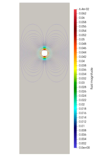
(a) $t=0.0s$

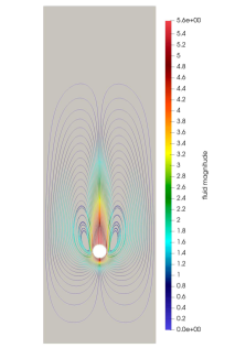
(b) $t=0.5s$

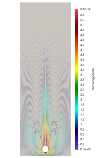
(c) $t=0.75s$

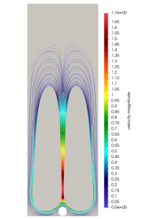
(d) $t=1.0s$

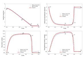
Figure 1: Evolution of the vertical position of mass center, vertical translational velocity, Reynolds number and translational kinetic energy. The red line are the present results, the green dotted and blue dotted lines correspond to results respectively taken from [19] and [18]. The streamlines and body position at four different time instants are represented.

We perform the same simulation for the $3$D validation. Initially, a sphere of radius $r=0.75$cm and density $\rho_{s}=1.12\frac{\mbox{g}}{\mbox{cm}^{3}}$ is located at $(0\mbox{cm},12.75\mbox{cm},0\mbox{cm})$ in a computational box of dimensions $[-4\mbox{cm},4\mbox{cm}]\times[0\mbox{cm},15\mbox{cm}]\times[-4\mbox{cm},4\mbox{cm}]$. The box is filled with a fluid of density $\rho_{f}=0.962\frac{\mbox{g}}{\mbox{cm}^{3}}$ and viscosity $\mu=1.13\frac{\mbox{g}}{\mbox{cm s}}$. The mesh size and the time step are set to $h=0.1$cm and $\Delta t=0.01$s. Regarding the lubrication force parameters, we fixed the width of the collision zone to $\rho=0.2625$cm and the stiffness parameter to $\epsilon_{\mathcal{F}}=5*10^{-6}$. The comparison of the present results to literature results [21] is given in figure 2. We obtain the same results for the vertical coordinate of the center of mass and the vertical translational velocity.

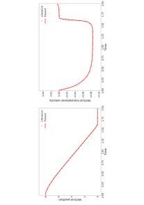
Figure 2: Comparison of the vertical position of the center of mass and vertical translational velocity observed in present results, red line, to literature results [21], dotted line.

5 Applications

5.1 Isolated object

In this subsection we simulate the interaction between a complex shaped body falling under the effect of gravity and the boundary of the computational domain filled with an incompressible Newtonian fluid in two and three dimensions.

For the first case, we consider a two-dimensional ellipse located in a channel of width $L=\frac{16}{130}$cm and infinite length. The channel contains a fluid of density $\rho_{f}=1.195\frac{\mbox{g}}{\mbox{cm}^{3}}$ and viscosity $\mu=0.305\frac{\mbox{g}}{\mbox{cm s}}$. The ellipse’s long and short axis are respectively set to $a=0.1$cm and $b=0.05$cm. Its density is equal to $\rho_{\mathcal{S}}=1.35\frac{\mbox{g}}{\mbox{cm}^{3}}$. Due to its initial orientation, set to $\theta=\frac{\pi}{3}$ with respect to the horizontal axis, the ellipse will collide with the right and left walls. To model these collisions the length of the lubrication zone is fixed at $\rho=0.05$cm and a stiffness parameter of $\epsilon_{\mathcal{F}}=10^{-5}$ is used. The simulation is performed using a mesh size $h=0.001$cm and a time step $\Delta t=0.001$s. Figure 3(a) shows the trajectory of the ellipse comparing it to literature [22]. This trajectory allows to observe that the ellipse first performs oscillations between the right and left wall before reaching a horizontal position, at the instant given by the black point. Then, it performs rotations close to a single wall. In present results, these rotations are taking place near the left wall, but in the reference article, they happen near the right wall. Given that the ellipse is in a horizontal position at the beginning of these rotations, any small difference in the collision model or the numerical resolution techniques can explain this difference. To show that the present results remain close to literature, we consider in figure 3(b) the symmetric trajectory for the rotations of [22]. This test case allows us to validate our implementation for the case of arbitrarily shaped bodies.

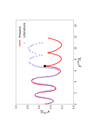
(a) Trajectory

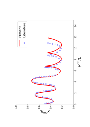
(b) Trajectory with symmetric results

Figure 3: The left graph plots the trajectory of the ellipse center of mass. The red line corresponds to the present results and the blue dotted line represents the literature results [22]. The right graph shows the same trajectory but compares it to rotations happening on the other wall.

The second case represents the simulation of a three-dimensional ellipsoid of density $\rho_{\mathcal{S}}=1.25\frac{\mbox{g}}{\mbox{cm}^{3}}$ and axis of length $a=0.4$cm and $b=c=0.2$cm falling in a rectangular computational domain filled with a fluid of density $\rho_{f}=1\frac{\mbox{g}}{\mbox{cm}^{3}}$ and viscosity $\mu=0.01\frac{\mbox{g}}{\mbox{cm s}}$. The dimensions of the domain are set to $[0\mbox{cm},1\mbox{cm}]\times[0\mbox{cm},8\mbox{cm}]\times[0\mbox{cm},0.4\mbox{cm}]$ and at $t=0$s the ellipsoid is located at $(0.5\mbox{cm},6\mbox{cm},0.2\mbox{cm})$ with its long axis oriented in vertical direction. The mesh size and time step of this simulation are $h=0.0125$cm and $\Delta t=0.001$s. The interactions between the ellipsoid and the boundary of the computational domain are modelled by defining a collision zone of width $\rho=0.04$cm and a stiffness parameter $\epsilon_{\mathcal{F}}=3*10^{-6}$. The evolution of the horizontal position of the sphere is shown in figure 4, and is compared to literature results [23]. The trajectories before and after the first interaction between the ellipsoid and the boundary of the computational domain, at time $t\approx 0.45$s, are in good agreement.

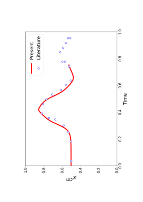
Figure 4: Evolution of the horizontal position of the center of the ellipsoid. The dotted line shows the literature results [23] and the red line represents the present results.

5.2 Multiple objects

Two disks falling in an incompressible fluid

Collisions between two spherical bodies placed on a same vertical line and falling under the effect of gravity, in a channel filled with incompressible Newtonian fluid, are known as the drafting, kissing and tumbling phenomenon. We consider two disks of radius $r=0.1$cm and density $\rho_{\mathcal{S}}=1.01\frac{\mbox{g}}{\mbox{cm}^{3}}$ placed in a fluid domain of dimensions $[0\mbox{cm},2\mbox{cm}]\times[0\mbox{cm},8\mbox{cm}]$. To have a slight asymmetry, necessary to speed up the insurgence of the phenomenon, the coordinates of the upper disk $\mathcal{S}1$ center are fixed at $(0.999\mbox{cm},7.2\mbox{cm})$ and those of the lower disk $\mathcal{S}2$ center at $(1.0\mbox{cm},6.8\mbox{cm})$. The fluid density and viscosity are respectively given by $\rho_{f}=1.0\frac{\mbox{g}}{\mbox{cm}^{3}}$ and $\mu=0.01\frac{\mbox{g}}{\mbox{cm s}}$. The simulation is performed on the time interval $[0\mbox{s},5\mbox{s}]$ with a time step equal to $\Delta t=0.001$s and a mesh size set to $h=0.01$. To model the drafting, kissing and tumbling phenomenon as in [24], one fixes the width of the collision zone at $\rho=0.0225$cm and uses stiffness parameters for the disk-disk and disk-fluid domain collisions given by $\epsilon=7*10^{-5}$ and $\epsilon_{\mathcal{F}}=5*10^{-5}$. Figure 5 shows the results of the simulation. When both disks are next to each other, the motion of the lower disk reduces the fluid pressure behind it and therefore the resistance of the fluid for the upper disk. As a result, the upper body falls faster until it collides with the lower one. The collision forces cause the separation of the disks which then move in opposite directions. Figure 5 also compares the vertical and horizontal position of the two disks over time to literature [24]. It can be observed that the results of the collision phase have same behavior. In the present simulation, the bodies fall faster to the bottom, therefore the separation phase takes place sooner than in literature results. This explains the differences on the graphes.

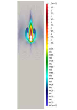
(a) $t=1.5s$

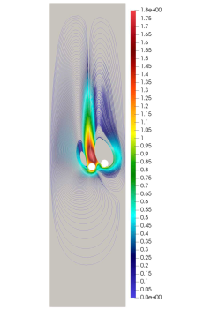
(b) $t=2.5s$

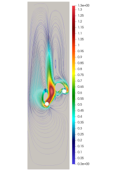
(c) $t=3.0s$

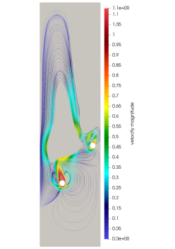
(d) $t=4.0s$

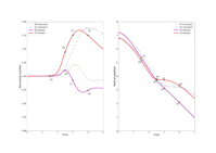
Figure 5: The upper figures show the position of the two disks as well as the streamlines at four different time instants. The lower graphs compare the evolution of the disks horizontal and vertical position to literature [24]. The solid lines correspond to present results and the dotted one to literature results.

$100$ disks falling in an incompressible fluid

We simulate the interactions between $100$ circular particles in two dimensions. The particles of radius $r=0.03125$cm and density $\rho_{\mathcal{S}}=1.1\frac{\mbox{g}}{\mbox{cm}^{3}}$ are placed in a vertical channel of height $2$cm and width $1$cm which is filled with a fluid of density $\rho_{f}=1.0\frac{\mbox{g}}{\mbox{cm}^{3}}$ and viscosity $\mu=0.01\frac{\mbox{g}}{\mbox{cm s}}$. At the beginning of the simulation, the fluid and the particles are at rest. Then the particles move towards the bottom of the domain under the effect of gravity. The initial configuration is given by the first figure of 6. We run the simulation on a time interval $[0\mbox{s},5.5\mbox{s}]$ and use a time step fixed at $\Delta t=0.002$s. The mesh size is given by $h=0.01$cm. The collision force is defined on range $\rho=0.025$cm. According to simulations of multiple objects interactions in the literature [25], the force intensity must be important to prevent the objects from overlapping. For this reason, we use stiffness parameters fixed at $\epsilon=5*10^{-6}$ and $\epsilon_{\mathcal{F}}=10^{-7}$. Figure 6 shows the position of the $100$ particles at four time instants. Due to the collision forces, the particles near the domain walls fall slower towards the bottom than the central particles. During the simulation the particles settle one onto the other on the bottom of the channel. At final time, almost all particles are in a stationary position and packed in a hexagonal lattice. Article [26] illustrates the same simulation but with different values of the parameters.

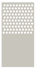
(a) $t=0.0s$

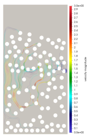
(b) $t=1.5s$

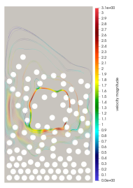
(c) $t=2.0s$

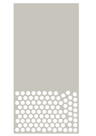
(d) $t=3.5s$

Figure 6: Streamlines and position at four different time instants of 100 disks falling under the effect of gravity in an incompressible Newtonian fluid.

Two objects in a flow

For this application we consider the motion of two circular particles in a symmetric stenotic artery in two dimensions. In contrast with the previous test cases, the particles do not fall under the effect of gravity, but the motion of the particles is due to a pressure difference between the inlet and the outlet. This simulation is presented in [27] and [28].

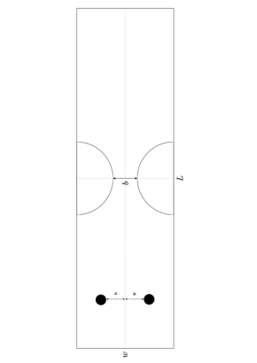
Figure 7: Geometry of symmetric stenotic artery

The geometry, given in figure 7, is a channel of length $L=32d$ and width $w=8d$. The centerlines are represented by dotted lines. The diameter $d$ of the particles is set to $d=8.5*10^{-4}$cm. To create the stenosis, the authors of [27] and [28] add two symmetrical protuberances shaped like semicircles. The radius of these protuberances depends on the width of the stenosis throat, which is fixed at $b=1.75d$. The fluid viscosity is set to $\mu=0.01\frac{\mbox{cm}^{2}}{\mbox{s}}$ and both fluid and particle densities are equal to $\rho_{f}=\rho_{\mathcal{S}}=1\frac{\mbox{g}}{\mbox{cm}^{3}}$. At time $t=0$, the fluid and the particles are at rest. Then the particles move towards the protuberances due to the pressure difference $\Delta p=541\mbox{Pa}$ between the inlet and outlet of the channel. The two particles are initially located at $8d$ to the left of the vertical centerline and asymmetrically with respect to the horizontal centerline: $h=2d+\frac{d}{4000}$ and $h^{\prime}=2d$. This slight asymmetry allows them to cross the stenosis throat. The mesh size and time step of the simulation are respectively set to $h=6.07*10^{-5}$cm and $\Delta t=10^{-5}$s. The time interval is $[0.0\mbox{s},0.01\mbox{s}]$. Collision forces are applied when the particles are close to the protuberances. The width of the collision zone is fixed at $\rho=0.0003$cm and the stiffness parameters of the particle-particle and particle-domain interactions are given by $\epsilon=10^{-11}$ and $\epsilon_{\mathcal{F}}=7.5*10^{-12}$. Figure 8 shows the trajectory of the two particles: they have a similar motion (snapshots $1$-$9$) until they get close to the stenosis throat (snapshot $10$). Since the width of the stenosis throat is too small to allow both particles to pass simultaneously, the upper particle stops and changes direction due to collision forces. Snapshot $11$ shows that it moves back to allow the lower particle passing the throat. Finally, the upper particle follows the lower particle through the artery (snapshots $11$-$17$). The same particle behavior is present in the cited articles. The particle trajectory after passing the stenosis throat depends on the initial configuration and the definition of collision parameters.

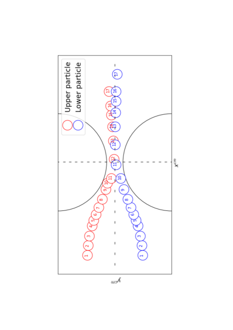
Figure 8: Position of two particles at different time instants.

Three-sphere swimmer in a Stokes flow

For the last test case, we consider the tilted three-sphere swimmer placed close to the boundary of a horizontal channel in a Stokes regime. The radius of the swimmer spheres is set to $r=1$cm and the length of its rods to $l=10$cm. The height and width of the computational domain are fixed at $h=150$cm and $w=40$cm. The mass center of the central sphere is initially located at $(15\mbox{cm},10\mbox{cm})$, and the density of the swimmer is given by $\rho_{\mathcal{S}}=0.1\frac{\mbox{g}}{\mbox{cm}^{3}}$. The fluid has a density equal to $\rho_{f}=1\frac{\mbox{g}}{\mbox{cm}^{3}}$ and a viscosity of $\mu=1\frac{\mbox{cm}^{2}}{\mbox{s}}$. The mesh size is set to $h=0.3$cm and the time step to $\Delta t=0.1$s. Due to the orientation of the swimmer at $t=0$s and due to its swimming strategy, leading to a straight motion, the swimmer gets closer to the boundary of the channel. Once its right sphere arrives in the collision zone of width $\rho=0.03$cm, lubrication forces, defined by a stiffness parameter set to $\epsilon_{\mathcal{F}}=5*10^{-8}$, are applied onto the swimmer, who starts to change direction. The swimmer rotates until its left sphere enters the collision zone, where the repulsive force applied on this sphere forces the swimmer to move upwards, away from the boundary. This behavior of the three-sphere swimmer close to the boundary is shown in figure 9.

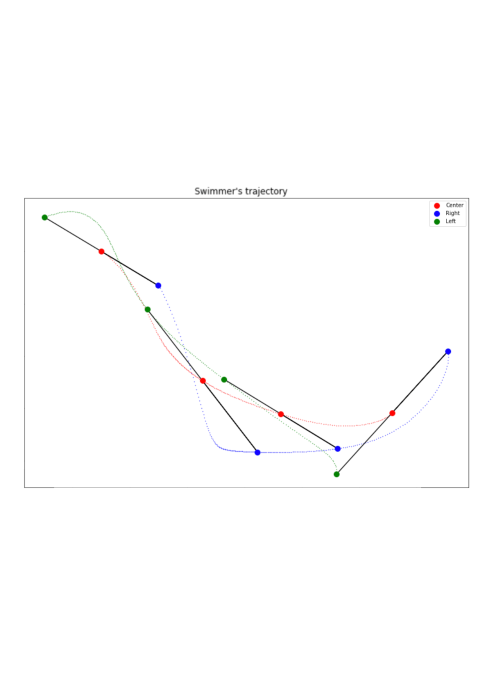
Figure 9: Behavior of the three-sphere swimmer close to the boundary of the computational domain.

Reproducibility

The validation benchmarks and all applications illustrated in this paper are available in a public GitHub repository [29]. All the results can be reproduced.

6 Conclusions

In this paper, we presented a repulsive collision-avoidance model for arbitrary-shaped bodies, where the definitions of force direction and magnitude are based on the computation of the distance function using the narrow-band fast marching method. The model is validated against literature results, with which we find good agreement. Various applications of two and three-dimensional cases are illustrated. In the appendix, we present a tool for the insertion of solid bodies into meshed domains, which allows simulations where the conforming treatment of the fluid-solid interface is required. Determining the optimal values for the collision parameters is still an open problem which could be tackled by anticipating the moments of collision and controlling the displacement of the bodies. The extension of this work to elastic bodies and collisions with multiple contact points will be the subject of an upcoming paper.

Appendix A Insertion of arbitrary solids into discretized fluid domains

In biological processes, such as particle transport in blood vessels, solid bodies move in geometrically complex domains. The reconstruction of such environments for numerical simulations is often image-based rather than relying on a CAD description, which complicates the mesh-fitted definition of solid bodies inside these environments. Hence, we have developed a tool allowing the insertion of arbitrary bodies in meshed domains with the identification of their geometric and material properties. The tool relies on the MMG library [30] feature that allows remeshing from a level-set function: given the initial triangulated environment and a level-set description of the solid body, it outputs a new triangulation that includes the solid, and where the interface between the two is conforming. In addition to this, we are able to insert multiple objects simultaneously, with prescribed position and orientation, and ensure that physical markers associated to the fluid and the solids are correctly transferred onto the new mesh.

The capabilities of the tool are illustrated in figures 10 and 11. Figure 10 shows a two-dimensional environment of complex geometry where a collection of objects have been successfully inserted without changes to their shapes. In particular all corners of the rectangular body have been recovered. Figure 11 illustrates a simpler three-dimensional domain where multiple bodies have been again successfully inserted. All three resulting meshes can be used for the simulation of fluid-solid interaction with collision treatment, as described in the first part of the paper.

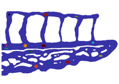
Figure 10: Creation of two-dimensional bodies inside a complex discretized environment.

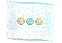
(a) Three-sphere swimmer

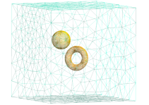
(b) Complex shaped bodies

Figure 11: Two cases showing the insertion of bodies in three dimensions.

References

- [1] R. Glowinski, Finite element methods for incompressible viscous flow, Vol. 9 of Handbook of Numerical Analysis, Elsevier, 2003.
-
[2]
A. Wachs, M. Uhlmann, J. Derksen, D. P. Huet,
Modeling
of short-range interactions between both spherical and non-spherical rigid
particles, in: Modeling Approaches and Computational Methods for
Particle-Laden Turbulent Flows, Elsevier, 2023, pp. 217–264.
doi:10.1016/B978-0-32-390133-8.00019-0.
URL https://linkinghub.elsevier.com/retrieve/pii/B9780323901338000190 -
[3]
R. Jain, S. Tschisgale, J. Fröhlich, A
collision model for DNS with ellipsoidal particles in viscous fluid,
International Journal of Multiphase Flow 120 (2019) 103087.
doi:10.1016/j.ijmultiphaseflow.2019.103087.
URL http://arxiv.org/abs/2201.04456 -
[4]
P. Singh, T. Hesla, D. Joseph,
Distributed
Lagrange multiplier method for particulate flows with collisions,
International Journal of Multiphase Flow 29 (3) (2003) 495–509.
doi:10.1016/S0301-9322(02)00164-7.
URL https://linkinghub.elsevier.com/retrieve/pii/S0301932202001647 -
[5]
A. Broms, A.-K. Tornberg, A Barrier
Method for Contact Avoiding Particles in Stokes Flow, preprint
(Jan. 2023).
URL http://arxiv.org/abs/2301.01666 -
[6]
A. Lefebvre, Numerical
simulation of gluey particles, ESAIM: Mathematical Modelling and Numerical
Analysis 43 (1) (2009) 53–80.
doi:10.1051/m2an/2008042.
URL http://www.esaim-m2an.org/10.1051/m2an/2008042 -
[7]
M. N. Ardekani, P. Costa, W.-P. Breugem, L. Brandt,
Numerical Study of the
Sedimentation of Spheroidal Particles, International Journal of
Multiphase Flow 87 (2016) 16–34.
doi:10.1016/j.ijmultiphaseflow.2016.08.005.
URL http://arxiv.org/abs/1602.05769 - [8] B. Muth, M.-K. Müller, M. Müller, P. Eberhard, S. Luding, Collision detection and administration methods for many particles with different sizes, in: 4th International Conference on Discrete Element Methods, DEM 4, Minerals Engineering Int., 2007, pp. 1–18.
-
[9]
B. Vemuri, L. Chen, L. Vu-Quoc, X. Zhang, O. Walton,
Efficient
and Accurate Collision Detection for Granular Flow Simulation,
Graphical Models and Image Processing 60 (6) (1998) 403–422.
doi:10.1006/gmip.1998.0479.
URL https://linkinghub.elsevier.com/retrieve/pii/S1077316998904798 - [10] M. Pouchol, A. Ahmad, B. Crespin, O. Terraz, A hierarchical hashing scheme for nearest neighbor search and broad-phase collision detection, Journal of Graphics, GPU, and Game Tools 14 (2) (2009) 45–59.
- [11] C. Ericson, Real-time collision detection, Crc Press, 2004.
-
[12]
J. A. Sethian, A fast
marching level set method for monotonically advancing fronts., Proceedings
of the National Academy of Sciences 93 (4) (1996) 1591–1595.
doi:10.1073/pnas.93.4.1591.
URL https://pnas.org/doi/full/10.1073/pnas.93.4.1591 - [13] L. Berti, V. Chabannes, L. Giraldi, C. Prud’homme, Fluid-rigid body interaction using the finite element method and ALE formulation: framework, implementation and benchmarkingPreprint.
- [14] L. Formaggia, A. Quarteroni (Eds.), Cardiovascular mathematics: modeling and simulation of the circulatory system, no. 1 in MS & A : modeling, simulation & applications, Springer, Milano, 2009.
-
[15]
B. Maury,
Direct
Simulations of 2D Fluid-Particle Flows in Biperiodic Domains,
Journal of Computational Physics 156 (2) (1999) 325–351.
doi:10.1006/jcph.1999.6365.
URL https://linkinghub.elsevier.com/retrieve/pii/S0021999199963659 -
[16]
H. Kanchi, A. Masud,
A 3D adaptive
mesh moving scheme, International Journal for Numerical Methods in Fluids
54 (6-8) (2007) 923–944.
doi:10.1002/fld.1512.
URL https://onlinelibrary.wiley.com/doi/10.1002/fld.1512 -
[17]
A. Najafi, R. Golestanian, A
Simplest Swimmer at Low Reynolds Number: Three Linked
Spheres, Physical Review E 69 (6) (2004) 062901.
doi:10.1103/PhysRevE.69.062901.
URL http://arxiv.org/abs/cond-mat/0402070 -
[18]
D. Wan, S. Turek,
Direct numerical
simulation of particulate flow via multigrid FEM techniques and the
fictitious boundary method, International Journal for Numerical Methods in
Fluids 51 (5) (2006) 531–566.
doi:10.1002/fld.1129.
URL https://onlinelibrary.wiley.com/doi/10.1002/fld.1129 -
[19]
L. Wang, Z. Guo, J. Mi,
Drafting,
kissing and tumbling process of two particles with different sizes,
Computers & Fluids 96 (2014) 20–34.
doi:10.1016/j.compfluid.2014.03.005.
URL https://linkinghub.elsevier.com/retrieve/pii/S0045793014001042 -
[20]
K. Usman, K. Walayat, R. Mahmood, N. Kousar,
Analysis of solid
particles falling down and interacting in a channel with sedimentation using
fictitious boundary method, AIP Advances 8 (6) (2018) 065201.
doi:10.1063/1.5035163.
URL http://aip.scitation.org/doi/10.1063/1.5035163 -
[21]
E. Zamora, L. Battaglia, M. Storti, M. Cruchaga, R. Ortega,
Numerical and
experimental study of the motion of a sphere in a communicating vessel system
subject to sloshing, Physics of Fluids 31 (8) (2019) 087106.
doi:10.1063/1.5098999.
URL http://aip.scitation.org/doi/10.1063/1.5098999 -
[22]
Z. Xia, K. W. Connington, S. Rapaka, P. Yue, J. J. Feng, S. Chen,
Flow
patterns in the sedimentation of an elliptical particle, Journal of Fluid
Mechanics 625 (2009) 249–272.
doi:10.1017/S0022112008005521.
URL https://www.cambridge.org/core/product/identifier/S0022112008005521/type/journal_article - [23] T.-W. Pan, R. Glowinski, G. P. Galdi, Direct simulation of the motion of a settling ellipsoid in Newtonian fluid, Journal of Computational and Applied Mathematics 149 (1) (2002) 71–82.
-
[24]
Z.-G. Feng, E. E. Michaelides,
The
immersed boundary-lattice Boltzmann method for solving fluid–particles
interaction problems, Journal of Computational Physics 195 (2) (2004)
602–628.
doi:10.1016/j.jcp.2003.10.013.
URL https://linkinghub.elsevier.com/retrieve/pii/S0021999103005758 -
[25]
T.-W. Pan, D. D. Joseph, R. Bai, R. Glowinski, V. Sarin,
Fluidization
of 1204 spheres: simulation and experiment, Journal of Fluid Mechanics 451
(2002) 169–191.
doi:10.1017/S0022112001006474.
URL https://www.cambridge.org/core/product/identifier/S0022112001006474/type/journal_article - [26] L. H. Juárez, R. Glowinski, T. Pan, Numerical simulation of fluid flow with moving and free boundaries, SeMA Journal: Boletín de la Sociedad Española de Matemática Aplicada (30) (2004) 49–102.
-
[27]
J. W. a. C. Shu,
Particulate
Flow Simulation Via a Boundary Condition-enforced Immersed
Boundary-lattice Boltzmann Scheme, Communications in Computational
Physics 7 (4) (2010) 793–812.
doi:10.4208/cicp.2009.09.054.
URL http://global-sci.org/intro/article_detail/cicp/7655.html -
[28]
H. Li, H. Fang, Z. Lin, S. Xu, S. Chen,
Lattice
Boltzmann simulation on particle suspensions in a two-dimensional symmetric
stenotic artery, Physical Review E 69 (3) (2004) 031919.
doi:10.1103/PhysRevE.69.031919.
URL https://link.aps.org/doi/10.1103/PhysRevE.69.031919 - [29] C. Prud’homme, V. Chabannes, T. Metivet, R. Hild, Trophime, S. Abdoulaye, T. Saigre, P. Ricka, L. Berti, C. Van Landeghem, feelpp/feelpp. doi:10.5281/ZENODO.5718297.
-
[30]
G. Balarac, F. Basile, P. Bénard, F. Bordeu, J.-B. Chapelier, L. Cirrottola,
G. Caumon, C. Dapogny, P. Frey, A. Froehly, G. Ghigliotti, R. Laraufie,
G. Lartigue, C. Legentil, R. Mercier, V. Moureau, C. Nardoni, S. Pertant,
M. Zakari,
Tetrahedral
remeshing in the context of large-scale numerical simulation and high
performance computing, MathematicS In Action 11 (1) (2022) 129–164.
doi:10.5802/msia.22.
URL https://msia.centre-mersenne.org/articles/10.5802/msia.22/