Leveraging Representations from Intermediate Encoder-blocks for Synthetic Image Detection

Abstract

The recently developed and publicly available synthetic image generation methods and services make it possible to create extremely realistic imagery on demand, raising great risks for the integrity and safety of online information. State-of-the-art Synthetic Image Detection (SID) research has led to strong evidence on the advantages of feature extraction from foundation models. However, such extracted features mostly encapsulate high-level visual semantics instead of fine-grained details, which are more important for the SID task. On the contrary, shallow layers encode low-level visual information. In this work, we leverage the image representations extracted by intermediate Transformer blocks of CLIP’s image-encoder via a lightweight network that maps them to a learnable forgery-aware vector space capable of generalizing exceptionally well. We also employ a trainable module to incorporate the importance of each Transformer block to the final prediction. Our method is compared against the state-of-the-art by evaluating it on 20 test datasets and exhibits an average +10.6% absolute performance improvement. Notably, the best performing models require just a single epoch for training ($\sim$8 minutes). Code available at GitHub.

Keywords synthetic image detection  $\cdot$ AI-generated image detection  $\cdot$ pre-trained intermediate features

1 Introduction

The recent advancements in the field of synthetic content generation is disrupting digital media communications, and pose new societal and economic risks [1]. Generative Adversarial Networks (GAN) [2], the variety of successor generative models [3] and the latest breed of Diffusion models [4] are capable of producing highly realistic images that humans are mostly incapable of distinguishing from real ones [5], and lead to grave risks ranging from fake pornography to hoaxes, identity theft, and financial fraud [6]. Therefore, it becomes extremely challenging to develop reliable synthetic content detection methods that can keep up with the latest generative models.

The scientific community has recently put a lot of effort on the development of automatic solutions to counter this problem [7, 6]. More precisely, the discrimination of GAN-generated from real images using deep learning models has gained a lot of interest, although it has been found that such approaches struggle to generalize to other types of generative models [8]. Synthetic Image Detection (SID) is typically performed based either on image-level [9, 10] or frequency-level features [11, 12, 13]. Also, there are methods [14, 15] that analyse the traces left by generative models to provide useful insights on how to address the SID task.

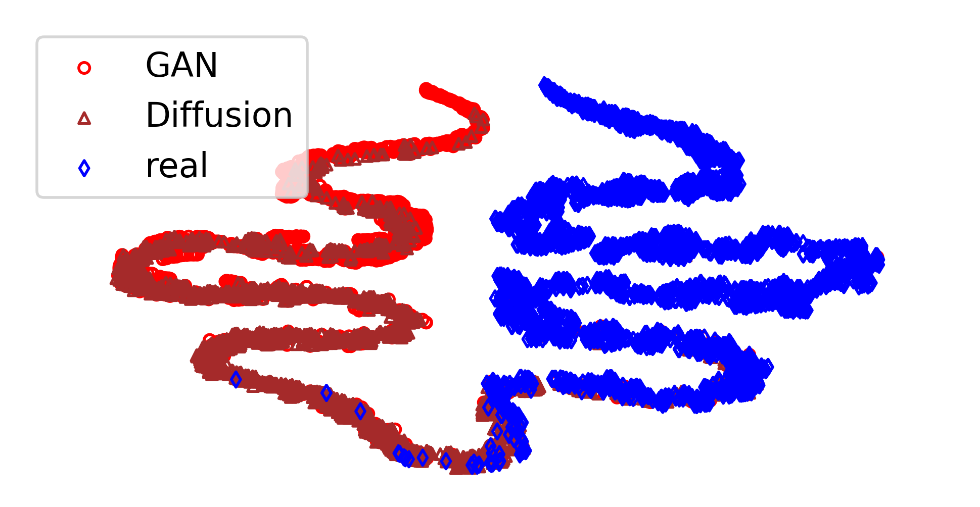
(a) RINE (Ours)

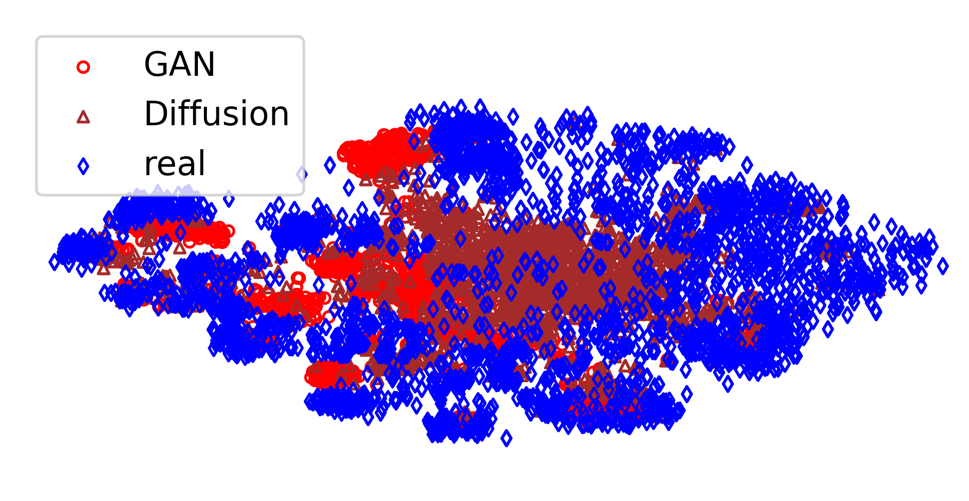
(b) UFD [16]

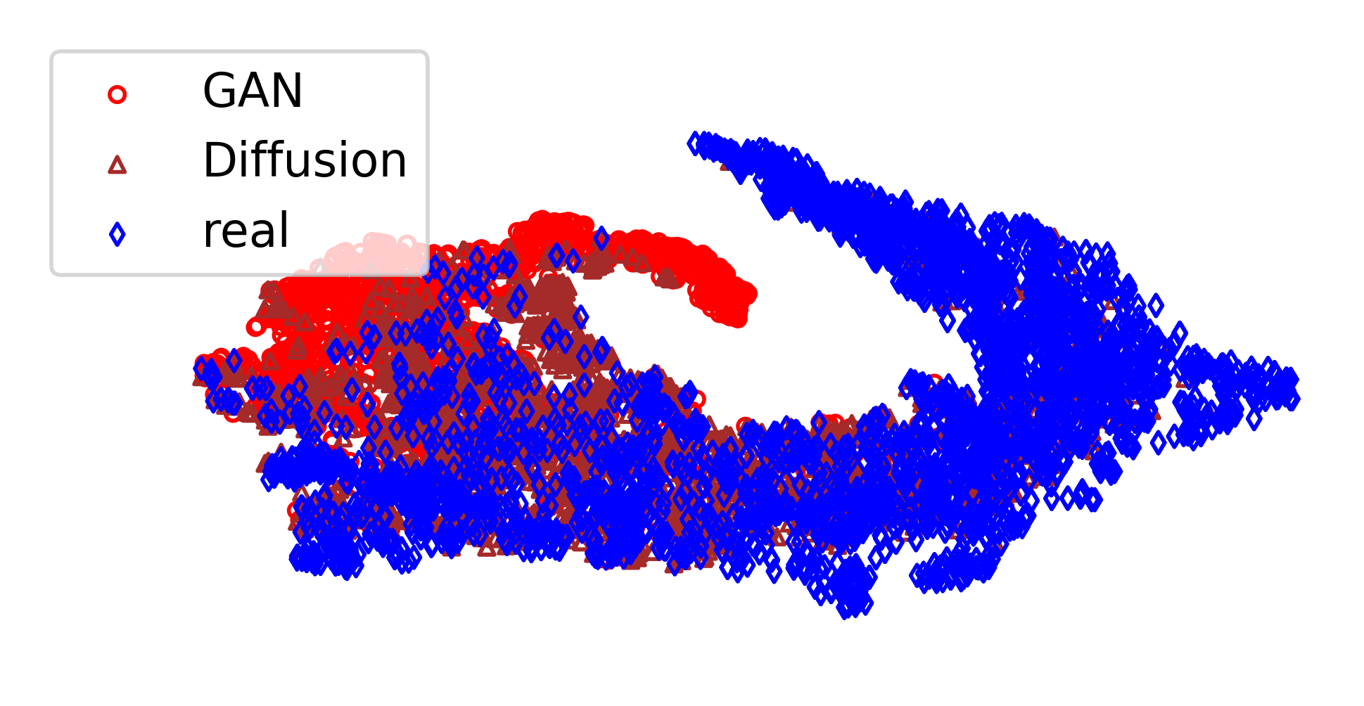
(c) Wang et al. [9]

Figure 1: Feature space visualization for unseen data with t-SNE.

Recently, the utilization of features extracted by foundation models, such as CLIP [17], has been found to yield surprisingly high performance in the SID task, with minimal training requirements [16]. However, this level of performance is associated with features extracted from the last model layer, which are known to capture high-level semantics. Instead, low-level image features deriving from intermediate layers, which are known to be highly relevant for synthetic image detection [18, 15], have not been explored to date, despite their potential to further boost performance.

To address the SID task more effectively, we propose the RINE model by leveraging Representations from Intermediate Encoder-blocks of CLIP. Specifically, we collect the image representations provided by intermediate Transformer blocks that carry low-level visual information and project them with learnable linear mappings to a forgery-aware vector space. Additionally, a Trainable Importance Estimator (TIE) module is used to incorporate the impact of each intermediate Transformer block in the final prediction. We train our models only on images generated by ProGAN (our experiments consider 1, 2, and 4 object classes for training) and evaluate it on 20 test datasets including images generated from GAN, Diffusion as well as other (deepfake, low-level vision, perceptual loss, DALL-E) generative models, surpassing by an average +10.6% the state-of-the-art performance. Figure 1 provides a comparison between the feature space of RINE and that of state-of-the-art methods, for GAN, Diffussion and real images, showcasing the discriminating ability of the proposed representation. Also, it is noteworthy that (i) we reach this level of performance with only 6.3M learnable parameters, (ii) trained only for 1 epoch, which requires $\sim$8 minutes, and (iii) we surpass the state-of-the-art by +9.4%, when training only on a single ProGAN object class, while the second-to-best model uses 20.

The paper is structured as follows. Section 2 reviews the related literature. Section 3 describes the proposed method. Section 4 presents the experimental setup. Section 5 illustrates the results. Section 6 outlines the conclusions.

2 Related work

Synthetic Image Detection (SID) has recently emerged as a special but increasingly interesting field of DeepFake or synthetic media detection (term often used as an umbrella term for all kinds of synthetic or manipulated content) [6, 7]. Early studies investigated fingerprints left by GAN generators, similarly to the fingerprints left by cameras [19], letting them not only to distinguish between real and synthetic images but also to attribute synthetic images to specific GAN generators [20, 21]. Other studies focused on GAN-based image-to-image translation detection [22] and face manipulation detection [23], but still the considered evaluation sets contained images generated from the same generators as the ones used for training, neglecting to assess generalizability. Such approaches have been shown to struggle with detecting images coming from unseen generators [8].

Subsequent works focused on alleviating this issue through patch-based predictions [10], auto-encoder based architectures [8] and co-occurrence matrices computed on the RGB image channels [24]. Next, Wang et al. [9] proposed a simple yet effective approach, based on appropriate pre- and post-processing as well as data augmentation, which is capable of generalizing well to many GAN generators by simply training on ProGAN images [25]. Additionally, traces of GAN generators in the frequency domain were exploited for effectively addressing the SID task [26, 11], while the use of frequency-level perturbation maps was proposed in [27] to force the detector to ignore domain-specific frequency-level artifacts. Image gradients estimated by a pre-trained CNN model have been shown to produce artifacts that can generalize well to unseen GAN generated images [28]. Removing the down-sampling operation from the first ResNet’s layer, that potentially eliminates synthetic traces, together with intense augmentation has shown promising results [15]. Another approach to improve generalization has been to select training images based on their perceptual quality; this was shown to be effective especially in cross-domain generalization settings [29].

Pre-trained features extracted by a foundation model were demonstrated to be surprisingly effective for the SID task, generalizing equally well on GAN and Diffusion model generated data [16]. Motivated by this success, we hypothesize that further performance gains are possible by leveraging representations from intermediate layers, which carry low-level visual information, in addition to representations from the final layer that primarily carry high-level semantic information. Our approach is different from deep layer aggregation that was explored in several computer vision tasks [30], as well as for deepfake detection [31], as we process the frozen layers’ outputs of a large-scale foundation model, while deep layer aggregation is a training technique that concatenates layer outputs to produce predictions during the training of a CNN model.

Finally, the performance drop of synthetic image detectors in real-world conditions typically performed when uploading content to social media (e.g., cropping and compression) has been analysed in [22, 15]. Our method is also effective in such conditions as demonstrated by the experimental results in Section 5.6.

3 Methodology

Figure 2 illustrates the main elements of the RINE architecture. We build upon the intermediate layer outputs of CLIP’s image encoder in order to train a lightweight SID model.

Figure 2: The RINE architecture. A batch of $b$ images is processed by CLIP’s image encoder. The concatenation of the $n$ $d$-dimensional CLS tokens (one from each intermediate stage, i.e., Transformer block) is first projected and then multiplied with the trainable importance scores of the intermediate stages, estimated by the Trainable Importance Estimator (TIE) module. Summation across the second dimension results in one feature vector per image. Finally, after the second projection and the consequent classification head modules, two loss functions are computed. The binary cross-entropy $\mathfrak{L}_{CE}$ directly optimizes the real vs. fake objective, while the contrastive loss $\mathfrak{L}_{Cont.}$ assists the training by forming a dense feature vector cluster per class.

3.1 Representations from Intermediate Encoder-blocks

Let us consider a batch of $b$ input images $\mathbf{X}\in\mathbb{R}^{b\times 3\times w\times h}$, with $w$ width and $h$ height. The images are first reshaped into a sequence of $p$ flattened image patches $\mathbf{X}_{p}\in\mathbb{R}^{b\times p\times(P^{2}\cdot 3)}$, where $P$ denotes patch side length and $p=w\cdot h/P^{2}$. Then, a $d$-dimensional linear mapping is considered on top of $\mathbf{X}_{p}$, the learnable $d$-dimensional CLS token is concatenated to the projected sequence, and positional embeddings are added to all $p+1$ tokens in order to construct the image encoder’s input, $\mathbf{Z}_{0}\in\mathbb{R}^{b\times(p+1)\times d}$. CLIP’s image encoder [17], being a standard Vision Transformer (ViT) [32], consists of $n$ successive Transformer encoder blocks [33], each processing the output of the previous block as shown in Equation 1:

$$\begin{split}\tilde{\mathbf{Z}_{l}}&=\text{MSA}(\text{LN}(\mathbf{Z}_{l-1}))+\mathbf{Z}_{l-1}\\ \mathbf{Z}_{l}&=\text{MLP}(\text{LN}(\tilde{\mathbf{Z}_{l}}))+\tilde{\mathbf{Z}_{l}}\end{split}$$ (1)

where $l$=1,…,n denotes the Transformer block’s index, $\mathbf{Z}_{l}\in\mathbb{R}^{b\times(p+1)\times d}$ denotes the $l$th Transformer block’s output, MSA denotes Multi-head Softmax Attention [33], LN denotes Layer Normalization [34], and MLP denotes a Multi-Layer Perceptron with two GELU [35] activated linear layers of $4\cdot d$ and $d$ number of units, respectively.

Finally, we define the tensor $\mathbf{K}$ containing the Representations from Intermediate Encoder-blocks (RINE), as the concatenation of the $n$ CLS tokens stemming from each of the $n$ Transformer blocks:

$$\mathbf{K}=\oplus\big{\{}\mathbf{Z}_{l}^{\text{[0]}}\big{\}}_{l=1}^{n}\in\mathbb{R}^{b\times n\times d}$$ (2)

where $\oplus$ denotes concatenation, and $\mathbf{Z}_{l}^{\text{[0]}}\in\mathbb{R}^{b\times 1\times d}$ denotes the CLS token from the output of Transformer block $l$. We keep CLIP, which produces these features, frozen during training and we use $\mathbf{K}$ to construct discriminative features for the SID task.

3.2 Trainable modules

The extracted representations $\mathbf{K}$ are processed by a projection network ($\mathfrak{Q}_{1}$ in Figure 2):

$$\mathbf{K}_{m}=\text{ReLU}(\mathbf{K}_{m-1}\mathbf{W}_{m}+\mathbf{b}_{m})\in\mathbb{R}^{b\times n\times d^{\prime}}$$ (3)

where $m$=1,…,q denotes the index of the network’s layer (with $\mathbf{K}_{0}=\mathbf{K}$), $\mathbf{W}_{m}\in\mathbb{R}^{d^{\prime}\times d^{\prime}}$ (except $\mathbf{W}_{1}\in\mathbb{R}^{d\times d^{\prime}}$) and $\mathbf{b}_{m}\in\mathbb{R}^{d^{\prime}}$ define the linear mapping, and ReLU denotes the Rectified Linear Unit [36] activation function. After each layer, dropout [37] with rate 0.5 is applied.

Additionally, each of the $d^{\prime}$ learned features can be more relevant for the SID task at various processing stages, thus we employ a Trainable Importance Estimator (TIE) module to adjust their impact to the final decision. More precisely, we consider a randomly-initialized learnable variable $\mathbf{A}=\{\alpha_{lk}\}\in\mathbb{R}^{n\times d^{\prime}}$ the elements of which will estimate the importance of feature $k$ at processing stage (i.e., Transformer block) $l$. This is then used to construct one feature vector per image, as a weighted average of features across processing stages:

$$\tilde{\mathbf{K}}=\sum_{l}^{n}\mathcal{S}(\mathbf{A})\otimes\mathbf{K}_{q}$$ (4)

where $\mathcal{S}$ denotes the Softmax activation function acting across the first dimension of $\mathbf{A}$, $\otimes$ denotes broadcasted Hadamard product, and summation is conducted across the dimension of Transformer blocks.

Finally, a second projection network ($\mathfrak{Q}_{2}$ in Figure 2) with the same architecture as the first one (cf. Equation 3) takes as input $\tilde{\mathbf{K}}$ and outputs $\tilde{\mathbf{K}}_{q}$, which is consequently processed by the classification head that predicts the final output (real/fake). The classification head consists of two $d^{\prime}\times d^{\prime}$ ReLU-activated dense layers and one $d^{\prime}\times 1$ dense layer which produces the logits.

3.3 Objective function

We consider the combination of two objective functions to optimize the parameters of the proposed model. The first is the binary cross-entropy loss [38], here denoted as $\mathfrak{L}_{CE}$, which measures the classification error and directly optimizes the main SID objective. The second is a contrastive loss function, specifically the Supervised Contrastive Learning loss (SupContrast) [39], which we here denote as $\mathfrak{L}_{Cont.}$, and is considered in order to assist the training process by bringing closer the feature vectors inside $\tilde{\mathbf{K}}_{q}$ that share targets and move apart the rest. We combine the two objective functions by a tunable factor $\xi$, as shown in Equation 5:

$$\mathfrak{L}=\mathfrak{L}_{CE}+\xi\cdot\mathfrak{L}_{Cont.}$$ (5)

4 Experimental setup

4.1 Datasets

Following the training protocol of related work [16, 9, 28], we use for training ProGAN [25] generated images and the corresponding real images of the provided dataset. Similarly with previous works [28, 27], we consider three settings with ProGAN-generated training data from 1 (horse), 2 (chair, horse) and 4 (car, cat, chair, horse) object classes. For testing, this is the first study to consider 20 datasets, with generated and real images, combining the evaluation datasets used in [16, 9, 28]. Specifically, the evaluation sets are from ProGAN [25], StyleGAN [40], StyleGAN2 [41], BigGAN [42], CycleGAN [43], StarGAN [44], GauGAN [45], DeepFake [23], SITD [46], SAN [47], CRN [48], IMLE [49], Guided [50], LDM [51] (3 variants), Glide [52] (3 variants), and DALL-E [53].

4.2 Implementation details

The training of RINE is conducted with batch size 128 and learning rate 1e-3 for only 1 epoch using the Adam optimizer. To assess the existence of potential benefit from further training we also conduct a set of experiments with 3, 5, 10, and 15 epochs (cf. Section 5.4). For each of the 3 training settings (1-class, 2-class, 4-class), we consider a hyperparameter grid to obtain the best performance, namely $\xi\in\{0.1,0.2,0.4,0.8\}$, $q\in\{1,2,4\}$, and $d^{\prime}\in~{}\{128,256,512,1024\}$. Additionally, we consider two CLIP variants, namely ViT-B/32 and L/14, for the extraction of representations. The models’ hyperparameters that result in the best performance (presented in Section 5) are illustrated in Table 1, along with the corresponding number of trainable parameters, and required training duration. For the training images, following the best practice in related work, we apply Gaussian blurring and $\mathtt{JPEG}$ compression with probability 0.5, then random cropping to 224$\times$224, and finally random horizontal flip with probability 0.5. The validation and test images are only center-cropped at 224$\times$224. Resizing is omitted both during training and testing as it is known to eliminate synthetic traces [15]. All experiments are conducted using one NVIDIA GeForce RTX 3090 Ti GPU.

# classes	backbone	$\xi$	$q$	$d$	$d^{\prime}$	# params.	training time
1	ViT-L/14	0.1	4	1024	1024	10.52M	$\sim$2 min.
2	ViT-L/14	0.2	4	1024	128	0.28M	$\sim$4 min.
4	ViT-L/14	0.2	2	1024	1024	6.32M	$\sim$8 min.

Table 1: Hyperparameter configuration of the best 1-, 2-, and 4-class models. The number of learnable parameters per model (in millions), and the training time (in minutes) is also reported.

4.3 State-of-the-art methods

The state-of-the-art SID methods we consider in our comparison include the following:

1. Wang [9]: A standard ResNet-50 [54] architecture pre-trained on ImageNet is fine-tuned on SID with appropriate selection of pre- and post-processing, as well as data augmentations.

2. Patch-Forensics [10]: A truncated (at block 2) Xception [55] pre-trained on ImageNet is fine-tuned on SID for each image patch, finally aggregating the individual patch-level predictions.

3. FrePGAN [27]: Frequency-level perturbation maps are generated by an adversarially trained network making fake images hard to distinguish from real ones, then a standard ResNet-50 [54] is trained on the SID task.

4. LGrad [28]: Image gradients, computed using a pre-trained deep network, are processed by a standard ResNet-50 [54] pre-trained on ImageNet, which is fine-tuned on the SID task.

5. DMID [15]: A ResNet-50 [54] without the down-sampling in the first layer and intense augmentation trained on the SID task.

6. Universal Fake Detector (UFD) [16]: Simple linear probing on top of (last layer) features extracted from CLIP’s ViT-L/14 [17] image encoder.

For all methods except FrePGAN, we compute performance metrics on the evaluation datasets presented in Section 4.1, using the publicly available checkpoints provided by their official repositories. For FrePGAN, that does not provide publicly available code and models, we present the scores that are reported in their paper [27].

4.4 Evaluation protocol

We evaluate the proposed architecture with accuracy (ACC) and average precision (AP) metrics on each test dataset, following previous works for comparability purposes. For the calculation of accuracy no calibration is conducted, we consider 0.5 as threshold to all methods. Best models are identified by the maximum sum ACC+AP. We also report the average (AVG) metric values across the test datasets to obtain summary evaluations.

5 Results

5.1 Comparative analysis

In Tables 2 and 3, we present the performance scores (ACC & AP respectively) of our method versus the competing ones. Our 1-class model outperforms all state-of-the-art methods irrespective of training class number. On average, we surpass the state-of-the-art by +9.4% ACC & +4.3% AP with the 1-class model, by +6.8% ACC & +4.4% AP with the 2-class model, and by +10.6% ACC & +4.5% AP with the 4-class model. In terms of ACC, we obtain the best score in 14 out of 20 test datasets, and simultaneously the first and second best performance in 10 of them. In terms of AP, we obtain the best score in 15 out of 20 test datasets, and simultaneously the first and second best performance in 14 of them. The biggest performance increase achieved by our method is on the SAN dataset [47] (+16.9% ACC).

		Generative Adversarial Networks								Low level vision			Perceptual loss			Latent Diffusion				Glide
		Pro-	Style-	Style-	Big-	Cycle-	Star-	Gau-	Deep-							200	200	100		100	50	100		AVG
method	# cl.	GAN	GAN	GAN2	GAN	GAN	GAN	GAN	fake	SITD	SAN		CRN	IMLE	Guided	steps	CFG	steps		27	27	10	DALL-E
Wang [9] (prob. 0.5)	20	100.0	66.8	64.4	59.0	80.7	80.9	79.2	51.3	55.8	50.0		85.6	92.3	52.1	51.1	51.4	51.3		53.3	55.6	54.2	52.5	64.4
Wang [9] (prob. 0.1)	20	100.0	84.3	82.8	70.2	85.2	91.7	78.9	53.0	63.1	50.0		90.4	90.3	60.4	53.8	55.2	55.1		60.3	62.7	61.0	56.0	70.2
Patch-Forensics [10]	$\dagger$	66.2	58.8	52.7	52.1	50.2	96.9	50.1	58.0	54.4	50.0		52.9	52.3	50.5	51.9	53.8	52.0		51.8	52.1	51.4	57.2	55.8
FrePGAN [27]	1	95.5	80.6	77.4	63.5	59.4	99.6	53.0	70.4	-*	-		-	-	-	-	-	-		-	-	-	-	-
FrePGAN [27]	2	99.0	80.8	72.2	66.0	69.1	98.5	53.1	62.2	-	-		-	-	-	-	-	-		-	-	-	-	-
FrePGAN [27]	4	99.0	80.7	84.1	69.2	71.1	99.9	60.3	70.9	-	-		-	-	-	-	-	-		-	-	-	-	-
LGrad [28]	1	99.4	96.1	94.0	79.6	84.6	99.5	71.1	63.4	50.0	44.5		52.0	52.0	67.4	90.5	93.2	90.6		80.2	85.2	83.5	89.5	78.3
LGrad [28]	2	99.8	94.5	92.1	82.5	85.5	99.8	73.7	61.5	46.9	45.7		52.0	52.1	72.1	91.1	93.0	91.2		87.1	90.5	89.4	88.7	79.4
LGrad [28]	4	99.9	94.8	96.1	83.0	85.1	99.6	72.5	56.4	47.8	41.1		50.6	50.7	74.2	94.2	95.9	95.0		87.2	90.8	89.8	88.4	79.7
DMID [15]	20	100.0	99.4	92.9	96.9	92.0	99.5	94.8	54.1	90.6**	55.5		100.0	100.0	53.9	58.0	61.1	57.5		56.9	59.6	58.8	71.7	77.6
UFD [16]	20	99.8	79.9	70.9	95.1	98.3	95.7	99.5	71.7	71.4	51.4		57.5	70.0	70.2	94.4	74.0	95.0		78.5	79.0	77.9	87.3	80.9
	1	99.8	88.7	86.9	99.1	99.4	98.8	99.7	82.7	84.7	72.4		93.4	96.9	77.9	96.9	83.5	97.0		83.8	87.4	85.4	91.9	90.3
RINE (Ours)	2	99.8	84.9	76.7	98.3	99.4	99.6	99.9	66.7	91.9	67.8		83.5	96.8	69.6	96.8	80.0	97.3		83.6	86.0	84.1	92.3	87.7
	4	100.0	88.9	94.5	99.6	99.3	99.5	99.8	80.6	90.6	68.3		89.2	90.6	76.1	98.3	88.2	98.6		88.9	92.6	90.7	95.0	91.5

* Hyphens denote scores that are neither reported in the corresponding paper nor the code and models are available in order to compute them.
** We applied cropping at 2000x1000 on SITD [46] for DMID [15] due to GPU memory limitations.
$\dagger$ Patch-Forensics has been trained on ProGAN data but not the on same dataset as the rest models. For more details please refer to [10].

Table 2: Accuracy (ACC) scores of baselines and our model across 20 test datasets. The second column (# cl.) presents the number of used training classes. Best performance is denoted with bold and second to best with underline. Our method yields +10.6% average accuracy compared to the state-of-the-art.

		Generative Adversarial Networks								Low level vision			Perceptual loss			Latent Diffusion				Glide
		Pro-	Style-	Style-	Big-	Cycle-	Star-	Gau-	Deep-							200	200	100		100	50	100		AVG
method	# cl.	GAN	GAN	GAN2	GAN	GAN	GAN	GAN	fake	SITD	SAN		CRN	IMLE	Guided	steps	CFG	steps		27	27	10	DALL-E
Wang [9] (prob. 0.5)	20	100.0	98.0	97.8	88.2	96.8	95.4	98.1	64.8	82.2	56.0		99.4	99.7	69.9	65.9	66.7	66.0		72.0	76.5	73.2	66.3	81.7
Wang [9] (prob. 0.1)	20	100.0	99.5	99.0	84.5	93.5	98.2	89.5	87.0	68.1	53.0		99.5	99.5	73.2	71.2	73.0	72.5		80.5	84.6	82.1	71.3	84.0
Patch-Forensics [10]	$\dagger$	94.6	79.3	77.6	83.3	74.7	99.5	83.2	71.3	91.6	39.7		99.9	98.9	58.7	68.9	73.7	68.7		50.6	52.8	48.4	66.9	74.1
FrePGAN [27]	1	99.4	90.6	93.0	60.5	59.9	100.0	49.1	81.5	-*	-		-	-	-	-	-	-		-	-	-	-	-
FrePGAN [27]	2	99.9	92.0	94.0	61.8	70.3	100.0	51.0	80.6	-	-		-	-	-	-	-	-		-	-	-	-	-
FrePGAN [27]	4	99.9	89.6	98.6	71.1	74.4	100.0	71.7	91.9	-	-		-	-	-	-	-	-		-	-	-	-	-
LGrad [28]	1	99.9	99.6	99.5	88.9	94.4	100.0	82.0	79.7	44.1	45.7		82.3	82.5	71.1	97.3	98.0	97.2		90.1	93.6	92.0	96.9	86.7
LGrad [28]	2	100.0	99.6	99.6	92.6	94.7	99.9	83.2	71.6	42.4	45.3		66.1	80.9	75.6	97.2	98.1	97.2		94.6	96.5	95.8	96.5	86.4
LGrad [28]	4	100.0	99.8	99.9	90.8	94.0	100.0	79.5	72.4	39.4	42.2		63.9	69.7	79.5	99.1	99.1	99.2		93.3	95.2	95.0	97.3	85.5
DMID [15]	20	100.0	100.0	100.0	99.8	98.6	100.0	99.8	94.7	99.8**	87.7		100.0	100.0	73.0	86.8	89.4	87.3		86.5	89.9	89.0	96.1	93.9
UFD [16]	20	100.0	97.3	97.5	99.3	99.8	99.4	100.0	84.4	89.9	62.6		94.5	98.3	89.5	99.3	92.5	99.3		95.3	95.6	95.0	97.5	94.3
	1	100.0	99.1	99.7	99.9	100.0	100.0	100.0	97.4	95.8	91.9		98.5	99.9	95.7	99.8	98.0	99.9		98.9	99.3	99.1	99.3	98.6
RINE (Ours)	2	100.0	99.5	99.6	99.9	100.0	100.0	100.0	96.4	97.5	93.1		98.2	99.8	95.7	99.9	98.0	99.9		98.9	99.0	98.8	99.6	98.7
	4	100.0	99.4	100.0	99.9	100.0	100.0	100.0	97.9	97.2	94.9		97.3	99.7	96.4	99.8	98.3	99.9		98.8	99.3	98.9	99.3	98.8

* Hyphens denote scores that are neither reported in the corresponding paper nor the code and models are available in order to compute them.
** We applied cropping at 2000x1000 on SITD [46] for DMID [15] due to GPU memory limitations.
$\dagger$ Patch-Forensics has been trained on ProGAN data but not the on same dataset as the rest models. For more details please refer to [10].

Table 3: Average precision (AP) scores of baselines and our model across 20 test datasets. The second column (# cl.) presents the number of used training classes. Best performance is denoted with bold and second to best with underline. Our method yields +4.5% mean average precision (mAP) compared to the state-of-the-art.

5.2 Ablations

In Table 4, we present an ablation study, where we remove three of RINE’s main components, namely the intermediate representations, the TIE, and the contrastive loss, one-by-one. To be more precise, “w/o intermediate” means that we use only the last layer’s features (equivalent to the SotA method [16]). We measure the RINE’s performance on 20 test datasets, after removing each of the three components, and present the average ACC and AP for the 1-, 2-, and 4-class models, as well as the average across the three models. In addition, we present the respective results in terms of generalization, namely for the non-GAN generators only. The results demonstrate the positive impact of all proposed components, as the full architecture achieves the best performance. Also, ablating intermediate representations yields the biggest performance loss reducing the metrics to the previous state-of-the-art levels (i.e., [16]), as expected.

	1-class			2-class			4-class			AVG
	ACC	AP		ACC	AP		ACC	AP		ACC	AP
all generators
w/o contr. loss	87.3	98.3		87.9	98.5		90.0	98.8		88.4	98.5
w/o TIE	85.0	97.8		86.4	98.5		90.5	98.8		87.3	98.3
w/o intermediate	78.9	93.1		81.1	94.7		82.5	94.8		80.8	94.2
full	90.3	98.6		87.7	98.7		91.5	98.8		89.8	98.7
non-GAN generators
w/o contr. loss	83.4	97.4		84.6	97.7		86.3	98.2		84.7	97.8
w/o TIE	80.0	96.6		82.0	97.8		87.0	98.2		83.0	97.5
w/o intermediate	73.4	90.0		76.3	92.4		77.0	92.4		75.5	91.6
full	87.2	98.0		84.3	98.1		88.3	98.3		86.6	98.1

Table 4: Ablation analysis compares the full architecture with it after removing the contrastive loss, the TIE module, and the intermediate representations.

5.3 Hyperparameter analysis

Figure 3(a)-(c) illustrates ACC & AP boxplots for ViT-B/32 vs. ViT-L/14 in the 1-, 2-, and 4-class settings. Each boxplot is built from 48 scores (ACC/AP) obtained from the experiments of all combinations of $\xi$, $q$, and $d^{\prime}$. It is clear that CLIP ViT-L/14 outperforms ViT-B/32, thus from now on we report results of ViT-L/14 only. Figure 3(d)-(f) illustrates the impact of the contrastive loss factor $\xi$, showing little variability across the different values, in all training settings.

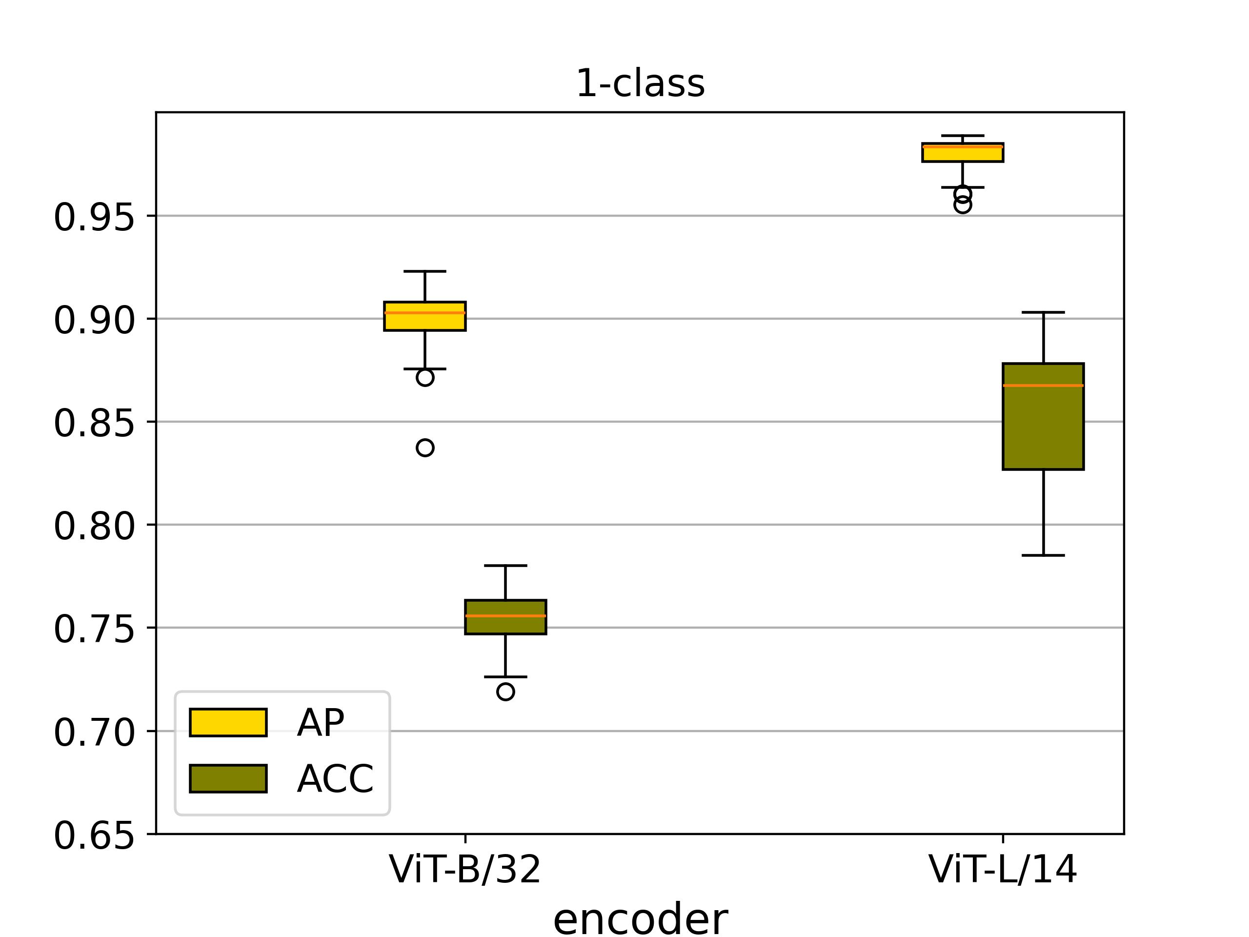
(a)

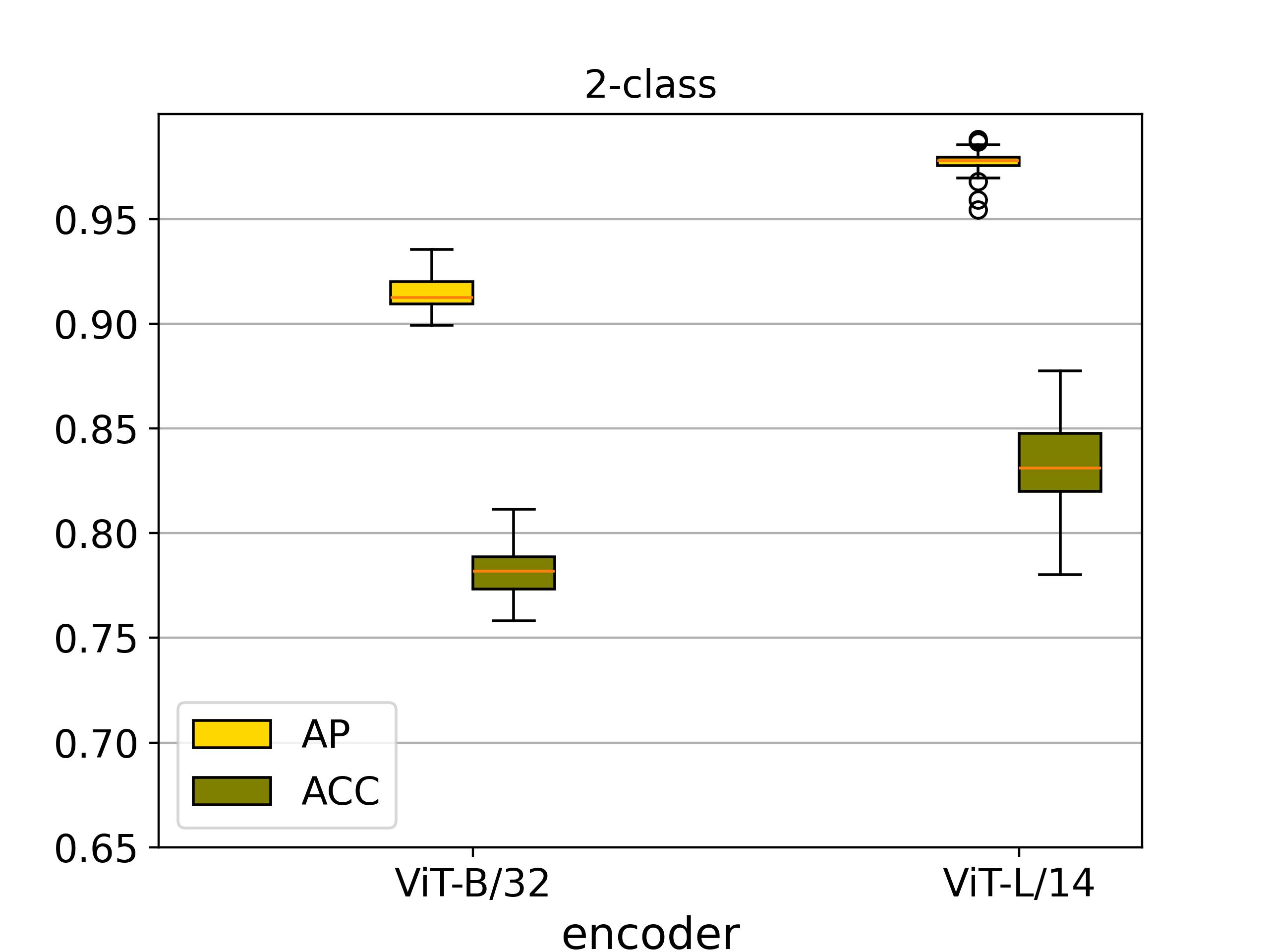
(b)

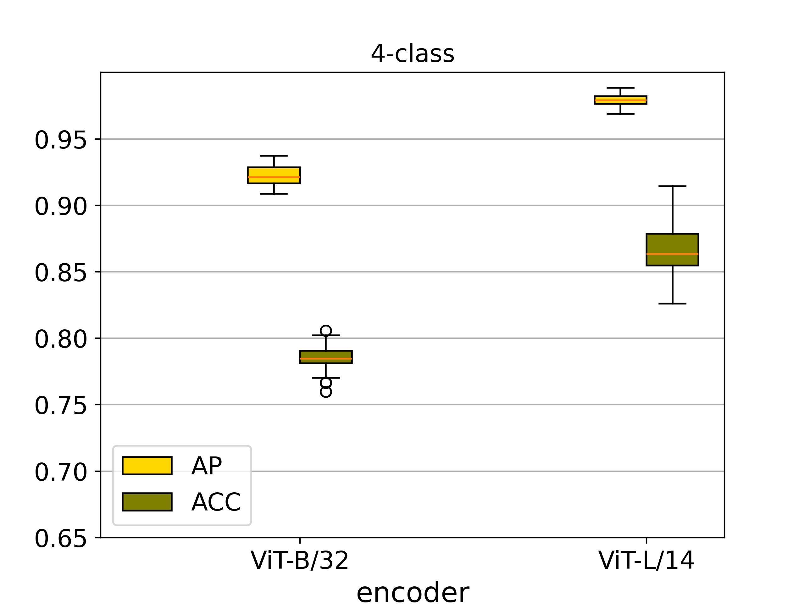
(c)

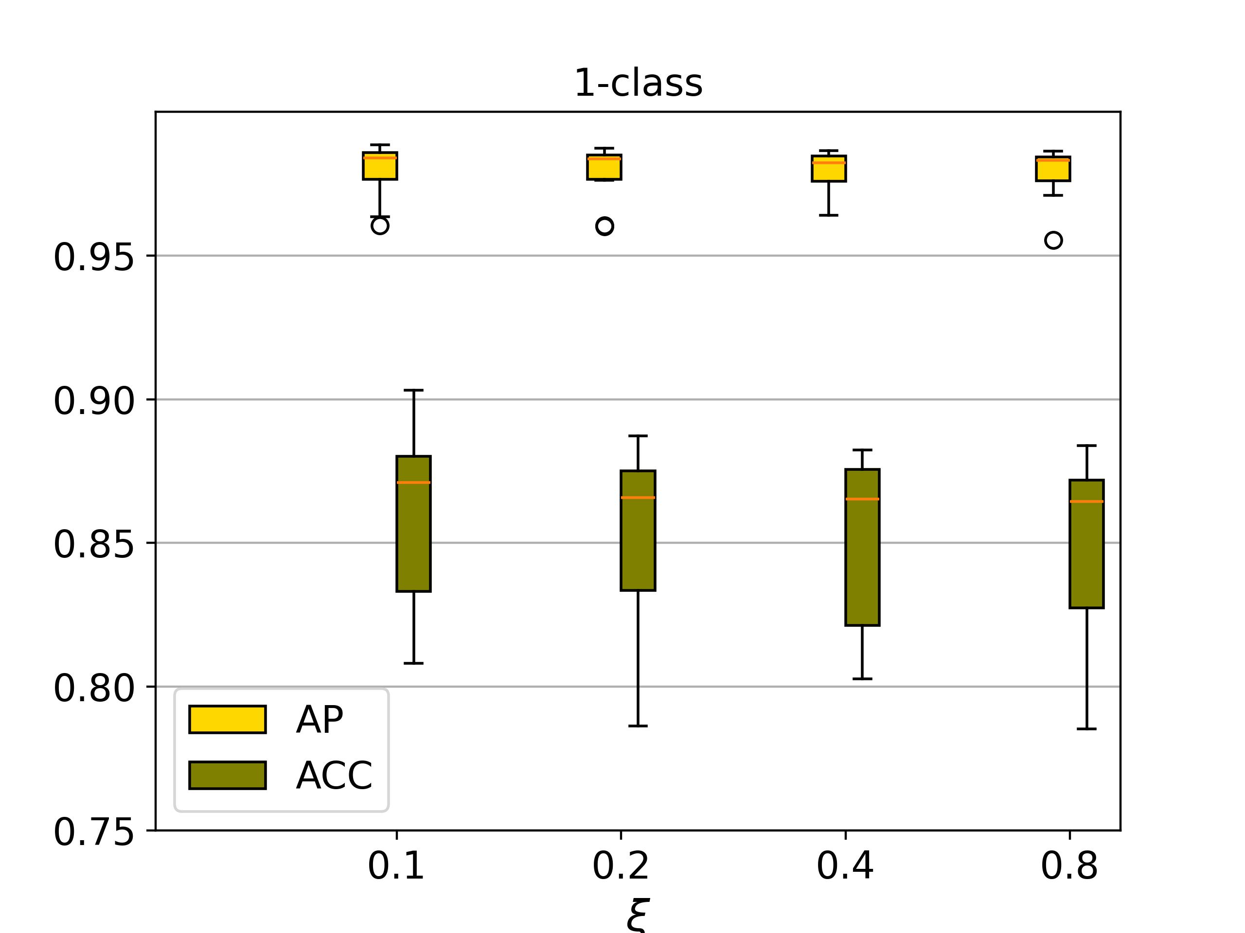
(d)

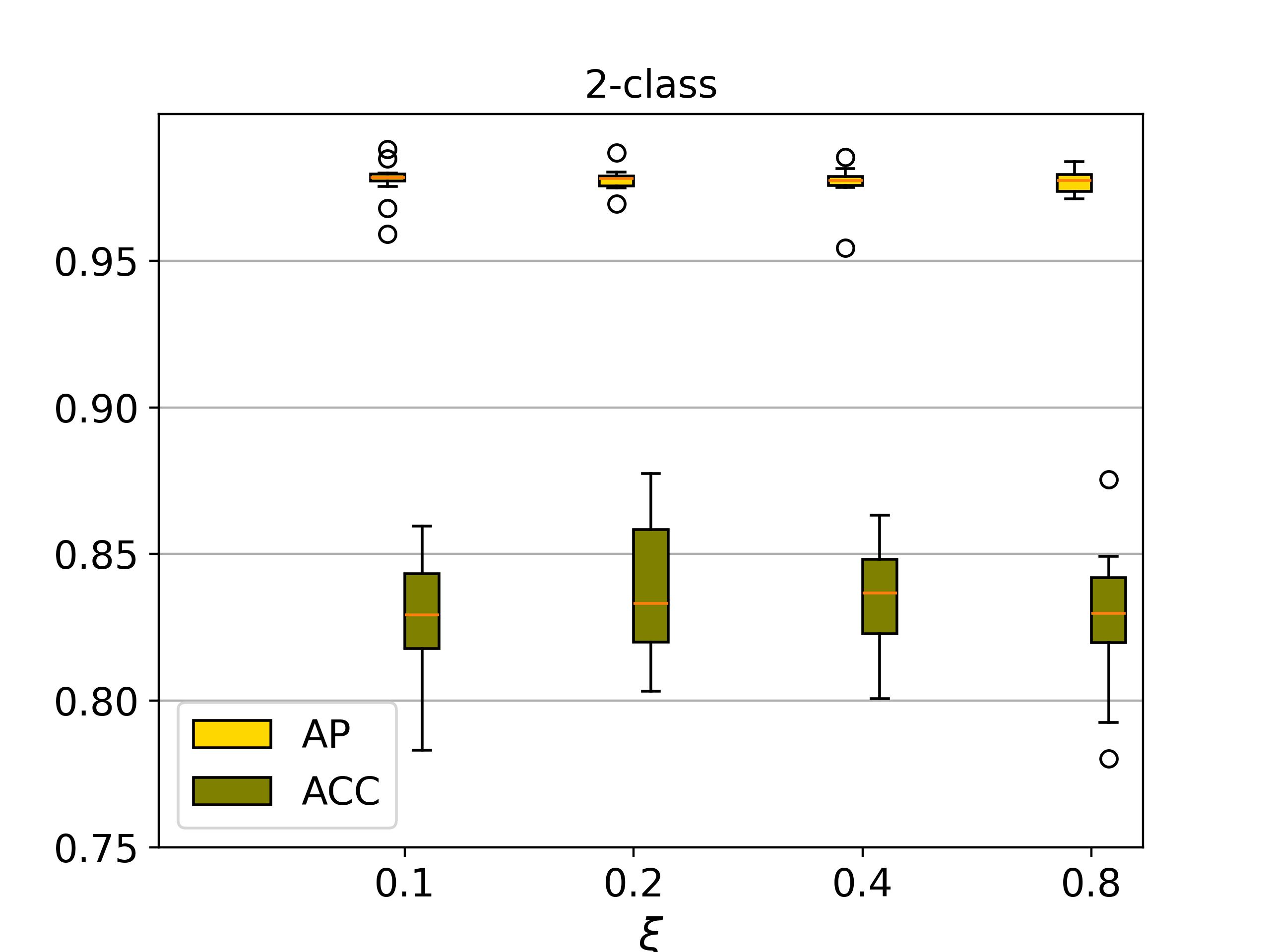
(e)

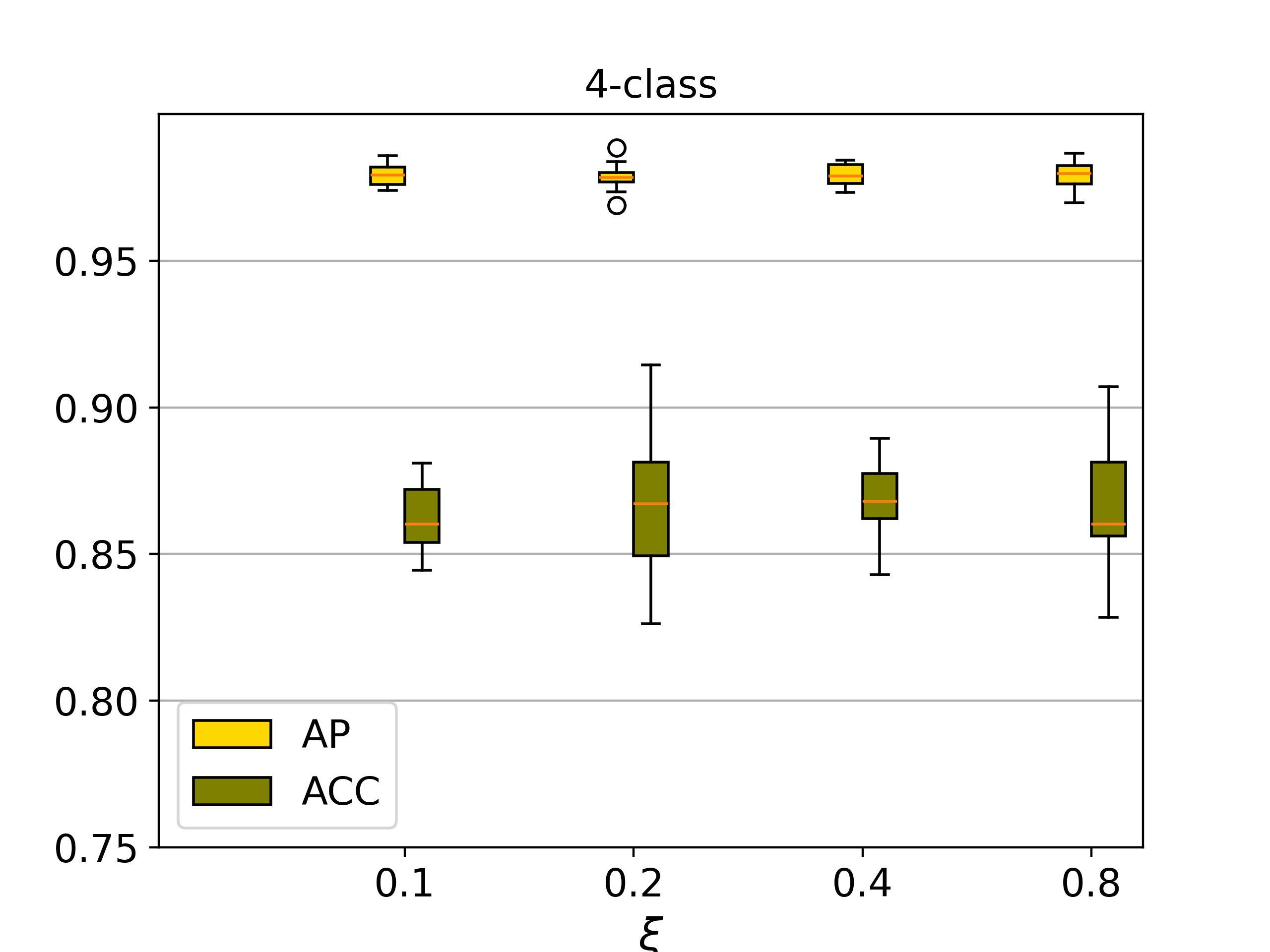
(f)

Figure 3: Boxplots of ACC and AP expressing the impact of image encoder ViT-B/32 vs. ViT-L/14 for the (a) 1-class, (b) 2-class, and (c) 4-class settings, and impact of the contrastive loss factor $\xi$ for the (d) 1-class, (e) 2-class, and (f) 4-class settings.

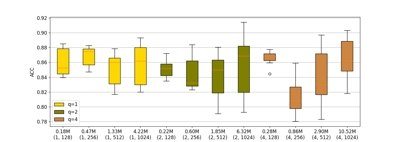
Figure 4: Boxplots of ACC for all different architectures of the trainable part of the model. X-axis shows the number of trainable parameters as well as the tuple ($q$, $d^{\prime}$).

Figure 4 presents ACC boxplots for each ($q$, $d^{\prime}$) combination of the trainable part of the model. For $q$=1, little variability is observed for different $d^{\prime}$ choices, while for $q$=2 and $q$=4, there is a slight performance increase with $d^{\prime}$ on average. The hyperparameter choices we have made for the proposed models are based on the maximum ACC & AP and not their average or distribution.

5.4 The effect of training duration

As stated in Section 4.2, the proposed models are trained for only one epoch. Here, we experimentally assess the potential benefit from further training. We identify the 3 best-performing configurations in the 1-epoch case for each of the 1-, 2-, and 4-class settings. Then, we train the corresponding models for 15 epochs and evaluate them in the 3rd, 5th, 10th, and 15th epoch (reducing learning rate by a factor of 10 at 6th and 11th epoch). Figure 5 presents their average and maximum performance, across the 20 test datasets, at different training stages. Neither the average nor the maximum performance improve if we continue training; instead, in the 1- and 4-class training settings performance drops.

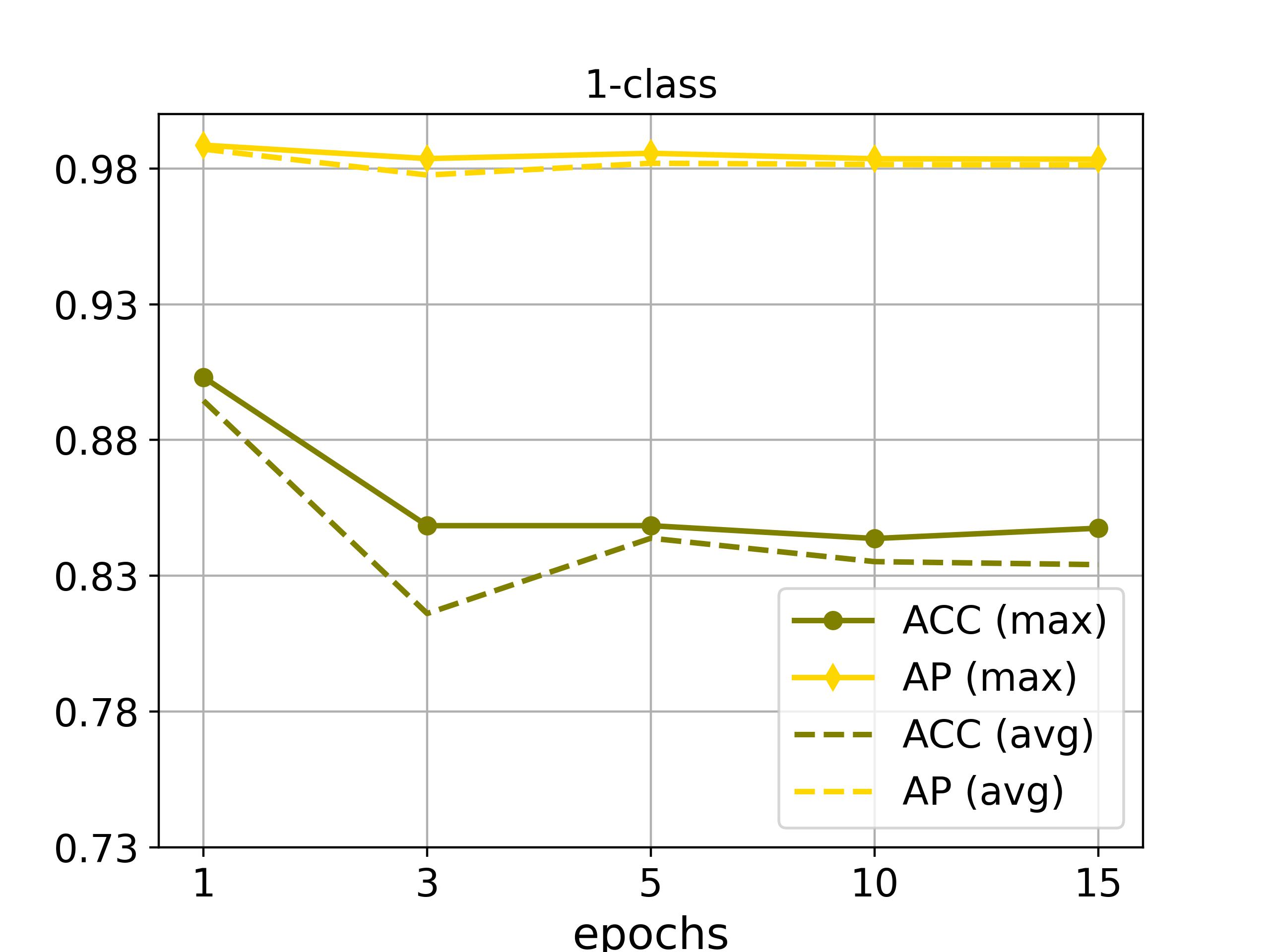
(a)

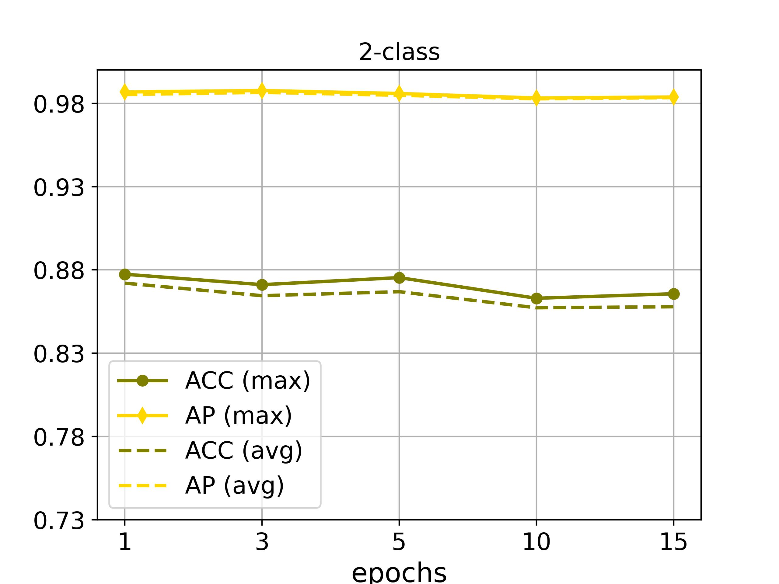
(b)

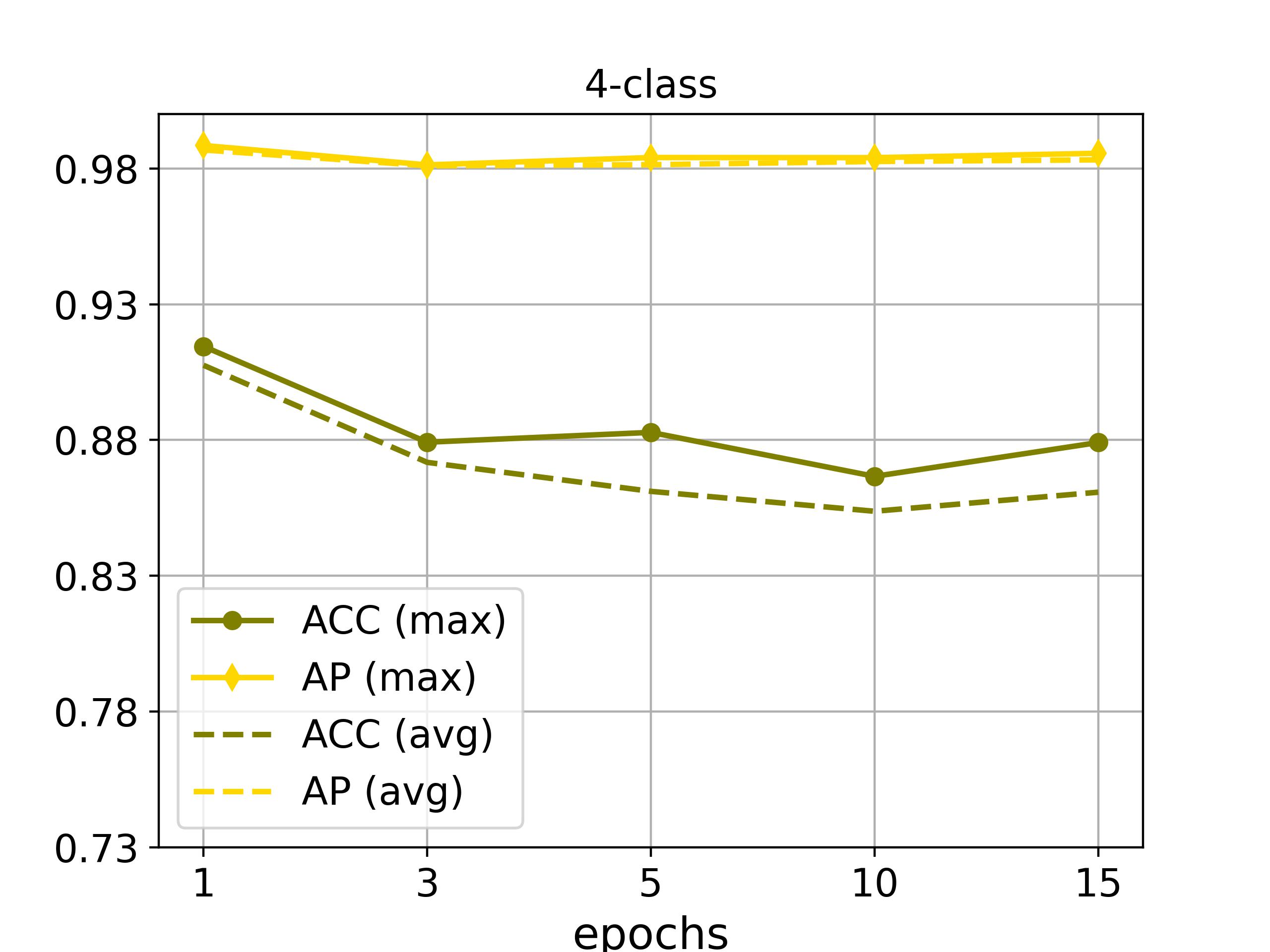
(c)

Figure 5: Maximum and average performance (ACC & AP) across the 20 evaluation datasets, of the 3 best-performing configurations at 3, 5, 10, and 15 epochs, for the (a) 1-class, (b) 2-class, and (c) 4-class training settings.

5.5 The effect of training set size

Here, we present a set of experiments in order to assess the effect of the training set size to our models’ performance. Specifically, we re-train (again for only one epoch) the best models (1-class, 2-class, 4-class) using 20%, 50%, 80%, and 100% of the training data. For the 1-class, these percentages correspond to 7K, 18K, 28K, and 36K images, for the 2-class to 14K, 36K, 57K, and 72K images, and for the 4-class to 28K, 72K, 115K, and 144K images. In Figure 6, we present the obtained performance (ACC & AP) on the 20 test datasets. We observe that the results are very close to each other, especially in terms of AP, showcasing the effectiveness of the proposed method even in limited training data settings.

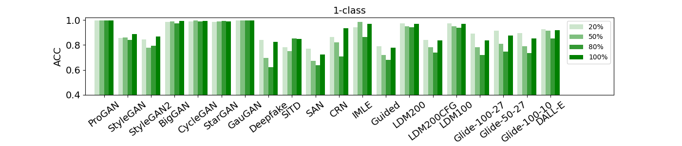
(a)

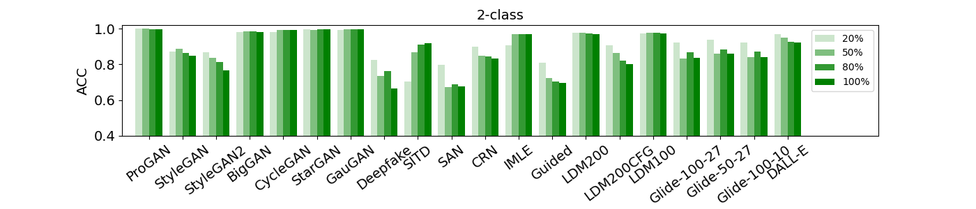
(b)

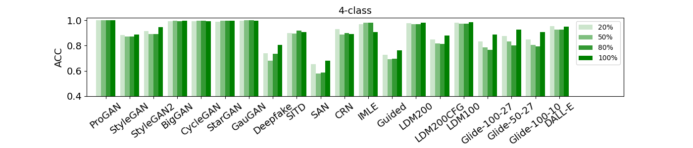
(c)

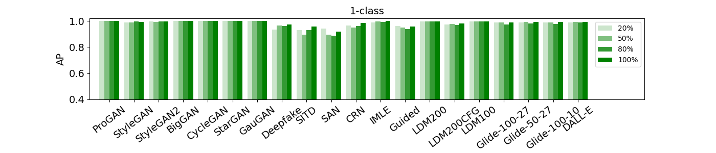
(d)

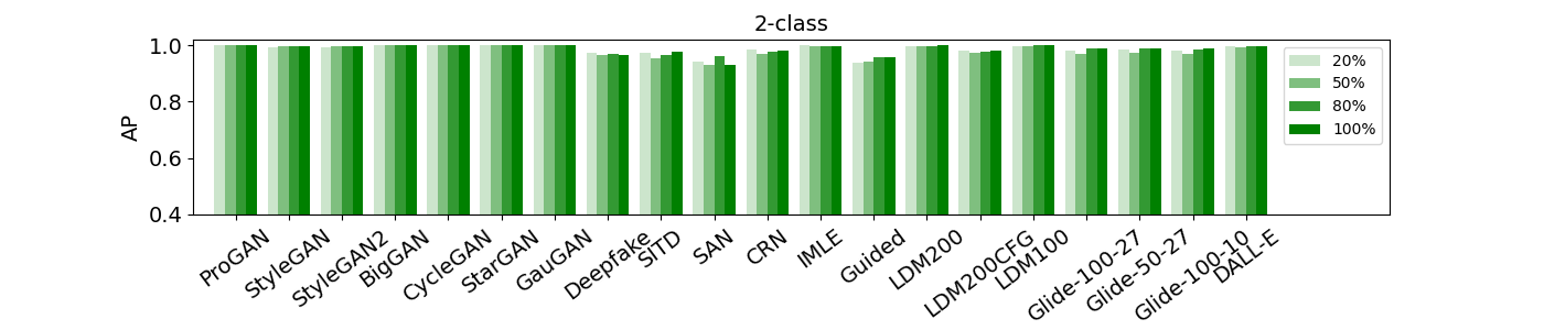
(e)

(f)

Figure 6: ACC on the 20 evaluation datasets when the proposed model is trained with 20%, 50%, 80%, and 100% of the training data, for the (a) 1-class, (b) 2-class, and (c) 4-class settings. In (d)-(f) the same for AP.

5.6 Robustness to common image perturbations

Following common practice [21, 9, 28, 16], in order to assess our method’s robustness to perturbations typically applied in social media, we assess our method’s performance after applying blurring, cropping, compression, noise addition, and their combination to each evaluation sample with 0.5 probability. The results in Table 5 indicate high robustness against cropping and compression, with minimal performance losses, and a good level of robustness against blurring and noise addition. Their combination seems to considerably reduce the models’ performance but at similar levels to that of current state-of-the-art without applying perturbations (cf. Table 2).

	Generative Adversarial Networks								Low level vision			Perceptual loss			Latent Diffusion				Glide
	Pro-	Style-	Style-	Big-	Cycle-	Star-	Gau-	Deep-							200	200	100		100	50	100		AVG
perturb.	GAN	GAN	GAN2	GAN	GAN	GAN	GAN	fake	SITD	SAN		CRN	IMLE	Guided	steps	CFG	steps		27	27	10	DALL-E
ACC
1-class
blur	96.3	78.3	76.2	91.3	90.3	94.1	93.9	72.3	88.9	61.4		83.8	86.5	77.1	93.3	78.5	93.2		77.5	79.0	77.0	88.9	83.9
crop	99.8	85.7	81.0	98.9	99.5	98.9	99.8	79.8	89.2	63.9		91.8	94.1	74.9	96.5	81.3	96.5		82.2	86.3	84.7	91.9	88.8
compress	99.1	81.2	77.3	96.9	99.0	98.4	99.7	78.7	89.2	62.8		88.6	96.1	72.1	94.4	76.3	94.2		79.3	81.0	81.6	89.0	86.7
noise	97.5	77.0	73.8	91.8	95.7	94.0	98.2	80.1	88.6	63.5		80.1	89.8	78.1	93.7	75.4	94.2		83.1	85.2	83.2	88.4	85.6
combined	88.8	72.3	71.7	80.7	87.7	90.1	89.3	75.3	88.3	62.8		76.3	80.0	80.2	87.4	72.2	88.4		78.4	81.1	79.2	82.6	80.6
no	99.8	88.7	86.9	99.1	99.4	98.8	99.7	82.7	84.7	72.4		93.4	96.9	77.9	96.9	83.5	97.0		83.8	87.4	85.4	91.9	90.3
2-class
blur	97.2	75.4	68.1	90.3	94.3	95.4	97.0	60.7	88.9	59.6		80.9	91.3	72.0	92.7	74.0	91.8		77.2	78.2	76.8	87.4	82.5
crop	99.8	81.3	72.5	98.0	99.4	99.6	99.8	64.5	89.7	61.4		85.3	96.9	67.2	97.0	79.2	97.2		83.1	85.3	83.4	92.5	86.7
compress	99.4	78.0	70.1	94.6	99.4	98.5	99.7	64.0	88.9	61.6		82.2	96.7	66.2	94.5	74.4	94.0		79.2	81.4	80.3	88.7	84.6
noise	97.7	74.2	67.5	89.5	96.2	93.5	98.8	69.0	88.6	62.6		73.3	88.4	71.7	92.8	71.0	91.6		79.5	80.3	79.5	87.1	82.6
combined	90.6	69.6	65.4	81.4	88.2	91.9	92.5	66.7	89.2	61.6		75.5	88.3	74.7	87.6	68.2	86.3		76.1	78.5	76.0	81.3	79.5
no	99.8	84.9	76.7	98.3	99.4	99.6	99.9	66.7	91.9	67.8		83.5	96.8	69.6	96.8	80.0	97.3		83.6	86.0	84.1	92.3	87.7
4-class
blur	97.7	86.9	90.4	93.9	91.5	98.5	95.1	72.3	91.7	57.8		81.0	81.6	77.6	92.8	81.2	92.3		83.2	87.2	85.2	92.2	86.5
crop	100.0	88.5	93.4	99.5	99.4	99.5	99.8	79.2	92.2	62.1		87.7	88.3	74.9	98.0	88.3	98.4		88.6	92.4	90.1	95.0	90.8
compress	99.9	87.5	89.2	98.1	99.2	99.6	99.7	72.8	91.4	61.9		88.0	93.0	70.6	95.2	79.8	95.9		85.8	88.4	87.2	91.2	88.7
noise	97.7	80.0	78.4	91.3	93.9	94.8	98.0	78.2	91.9	59.6		71.9	79.8	74.5	92.5	74.8	92.7		83.6	86.0	84.2	88.1	84.6
combined	91.9	75.8	78.9	82.6	88.7	91.2	92.9	72.5	92.5	58.7		77.5	85.0	79.1	89.1	73.4	89.2		82.8	85.2	83.5	82.5	82.7
no	100.0	88.9	94.5	99.6	99.3	99.5	99.8	80.6	90.6	68.3		89.2	90.6	76.1	98.3	88.2	98.6		88.9	92.6	90.7	95.0	91.5
AP
1-class
blur	99.7	94.6	93.6	97.6	98.6	99.5	99.8	93.2	96.1	76.1		94.1	98.9	91.0	98.6	91.2	98.6		93.1	94.0	92.9	96.8	94.9
crop	100.0	98.8	99.5	99.9	100.0	99.9	100.0	96.9	96.5	83.5		98.2	99.9	95.3	99.8	98.0	99.8		99.1	99.4	99.4	99.3	98.2
compress	100.0	98.5	99.0	99.7	99.9	99.9	100.0	96.1	96.0	82.3		95.9	99.6	94.0	99.7	96.2	99.7		98.6	98.8	98.8	99.1	97.6
noise	99.8	92.5	93.0	98.2	99.2	98.7	99.9	89.1	95.8	82.9		90.6	96.9	95.0	99.0	92.6	99.1		96.8	97.3	96.5	97.7	95.5
combined	97.8	84.9	84.3	92.1	97.0	97.6	98.2	84.0	95.9	77.8		87.2	94.6	92.2	95.7	84.0	96.0		88.7	89.9	87.7	92.1	90.9
no	100.0	99.1	99.7	99.9	100.0	100.0	100.0	97.4	95.8	91.9		98.5	99.9	95.7	99.8	98.0	99.9		98.9	99.3	99.1	99.3	98.6
2-class
blur	99.8	94.7	92.2	97.7	99.6	99.8	99.9	90.6	96.2	77.3		90.7	98.2	91.2	98.8	91.3	98.5		93.8	93.9	93.4	97.4	94.7
crop	100.0	99.4	99.4	99.9	100.0	100.0	100.0	95.8	96.8	86.4		97.4	99.7	94.7	99.9	98.1	99.9		98.8	99.0	98.9	99.6	98.2
compress	100.0	99.1	98.8	99.7	100.0	100.0	100.0	94.9	96.3	85.2		96.5	99.7	94.1	99.7	96.0	99.7		98.3	98.5	98.4	99.2	97.7
noise	99.8	93.1	91.7	98.2	99.5	99.3	99.9	84.6	96.4	84.3		91.7	98.0	93.7	99.2	91.7	99.2		97.2	96.9	96.7	98.3	95.5
combined	97.8	84.8	81.0	92.8	98.0	98.2	98.5	78.3	96.6	77.2		87.3	96.2	90.4	96.5	84.1	95.8		90.4	91.4	90.7	93.4	91.0
no	100.0	99.5	99.6	99.9	100.0	100.0	100.0	96.4	97.5	93.1		98.2	99.8	95.7	99.9	98.0	99.9		98.9	99.0	98.8	99.6	98.7
4-class
blur	99.9	97.1	98.4	98.7	99.6	99.9	99.8	93.5	97.3	74.2		95.1	99.5	90.5	98.4	93.1	98.1		94.4	96.0	94.9	97.7	95.8
crop	100.0	99.5	100.0	99.9	100.0	100.0	100.0	97.8	96.6	86.9		97.5	99.7	95.6	99.8	98.3	99.9		99.0	99.4	99.0	99.5	98.4
compress	100.0	99.4	99.9	99.9	100.0	100.0	100.0	96.1	97.2	86.0		95.4	99.5	94.3	99.6	96.0	99.6		98.6	98.9	98.6	98.8	97.9
noise	99.9	96.5	97.6	98.7	98.9	99.1	99.9	88.0	97.4	86.5		82.7	91.5	94.5	99.0	93.0	98.8		97.8	98.1	97.8	98.0	95.7
combined	98.2	89.4	91.7	93.3	97.9	98.2	98.4	82.1	97.3	77.9		88.1	94.6	93.3	96.6	87.6	96.3		92.4	94.9	93.7	93.5	92.8
no	100.0	99.4	100.0	99.9	100.0	100.0	100.0	97.9	97.2	94.9		97.3	99.7	96.4	99.8	98.3	99.9		98.8	99.3	98.9	99.3	98.8

Table 5: Performance (ACC & AP) after applying common image perturbations.

5.7 Importance of intermediate stages

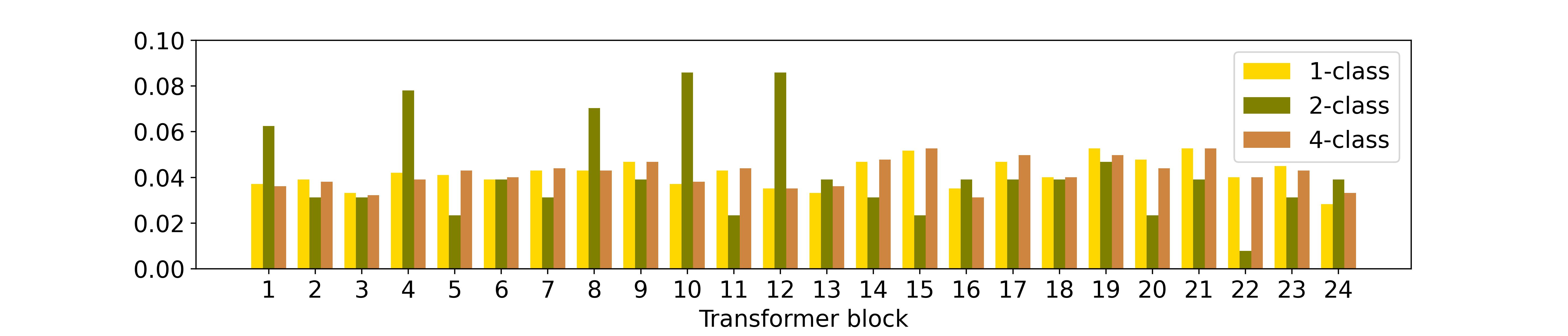
Figure 7: Frequency ($f_{l}$) of each Transformer block obtaining the maximum importance over feature elements.

In Section 5.2, it was demonstrated that the intermediate representations comprise the most important component of the proposed method as their incorporation produces the biggest performance increase. Here, we estimate the importance of each intermediate stage (i.e., Transformer block) by analysing the importance scores $\mathbf{A}=\{\alpha_{lk}\}$ estimated by the TIE module (cf. Equation 4) as follows:

$$l^{*}_{k}=\underset{l}{\mathrm{argmax}}(\alpha_{lk})\text{, for $k$=1,\ldots,$d^{\prime}$}$$

$$f_{l}=\frac{\mid\{k\mid l^{*}_{k}=l\}\mid}{d^{\prime}}\text{, for $l$=1,\ldots,n}$$

Figure 7 illustrates the frequency $f_{l}$ of Transformer block $l$ obtaining maximum importance, for $l$=1,…,$n$. For the 1-class and 4-class models $n$=24 and $d^{\prime}$=1024, while for the 2-class model $n$=24 and $d^{\prime}$=128. We observe that there are many Transformer blocks obtaining higher maximum importance frequency than the last one in all training settings, supporting the proposed method’s motivation.

5.8 The effect of training data origin on detecting Diffusion images

We additionally assess our method’s performance on Diffusion data produced by commercial tools, and more precisely on the Synthbuster dataset [56]. Due to the images’ size we consider the ten-crop validation technique and average the predictions. Table 6 illustrates RINE’s performance on Synthbuster when trained on ProGAN data from [9], and on Latent Diffusion Model (LDM) data from [15]. As expected training on Diffusion data provides big performance gains.

training set	DALL-E 2	DALL-E 3	SD1.3	SD1.4	SD2	SD XL	Glide	Firefly	Midjourney
ProGAN (from [9])	64.6/86.7	21.1/30.7	66.3/91.3	65.8/91.4	49.0/66.8	53.3/73.4	42.6/55.7	70.8/99.3	34.2/39.5
LDM (from [15])	89.8/96.2	47.2/32.5	96.4/100.0	96.4/100.0	93.5/98.5	96.3/99.8	90.0/96.3	85.3/93.4	92.4/97.4

Table 6: Performance (ACC/AP) of our method on Synthbuster.

6 Conclusions

In this work, inspired by the recent advances on the use of large-scale pre-trained visual features, we propose RINE that leverages representations from intermediate encoder-blocks of CLIP, as more effective to the SID task. Our comprehensive experimental study demonstrates the superiority of our approach compared to the state of the art. As an added benefit, the proposed approach requires only one epoch, translating to $\sim$8 minutes of training time, and limited training data to achieve maximum performance, while it is robust to common image transformations.

References

- [1] Stamatis Karnouskos. Artificial intelligence in digital media: The era of deepfakes. IEEE Transactions on Technology and Society, 1(3):138–147, 2020.
- [2] Ian Goodfellow, Jean Pouget-Abadie, Mehdi Mirza, Bing Xu, David Warde-Farley, Sherjil Ozair, Aaron Courville, and Yoshua Bengio. Generative adversarial nets. Advances in neural information processing systems, 27, 2014.
- [3] Guillermo Iglesias, Edgar Talavera, and Alberto Díaz-Álvarez. A survey on gans for computer vision: Recent research, analysis and taxonomy. Computer Science Review, 48:100553, 2023.
- [4] Florinel-Alin Croitoru, Vlad Hondru, Radu Tudor Ionescu, and Mubarak Shah. Diffusion models in vision: A survey. IEEE Transactions on Pattern Analysis and Machine Intelligence, 2023.
- [5] Zeyu Lu, Di Huang, Lei Bai, Jingjing Qu, Chengyue Wu, Xihui Liu, and Wanli Ouyang. Seeing is not always believing: Benchmarking human and model perception of ai-generated images. In Thirty-seventh Conference on Neural Information Processing Systems Datasets and Benchmarks Track, 2023.
- [6] Ruben Tolosana, Ruben Vera-Rodriguez, Julian Fierrez, Aythami Morales, and Javier Ortega-Garcia. Deepfakes and beyond: A survey of face manipulation and fake detection. Information Fusion, 64:131–148, 2020.
- [7] Yisroel Mirsky and Wenke Lee. The creation and detection of deepfakes: A survey. ACM Computing Surveys (CSUR), 54(1):1–41, 2021.
- [8] Davide Cozzolino, Justus Thies, Andreas Rössler, Christian Riess, Matthias Nießner, and Luisa Verdoliva. Forensictransfer: Weakly-supervised domain adaptation for forgery detection. arXiv preprint arXiv:1812.02510, 2018.
- [9] Sheng-Yu Wang, Oliver Wang, Richard Zhang, Andrew Owens, and Alexei A Efros. Cnn-generated images are surprisingly easy to spot… for now. In Proceedings of the IEEE/CVF conference on computer vision and pattern recognition, pages 8695–8704, 2020.
- [10] Lucy Chai, David Bau, Ser-Nam Lim, and Phillip Isola. What makes fake images detectable? understanding properties that generalize. In Computer Vision–ECCV 2020: 16th European Conference, Glasgow, UK, August 23–28, 2020, Proceedings, Part XXVI 16, pages 103–120. Springer, 2020.
- [11] Joel Frank, Thorsten Eisenhofer, Lea Schönherr, Asja Fischer, Dorothea Kolossa, and Thorsten Holz. Leveraging frequency analysis for deep fake image recognition. In International conference on machine learning, pages 3247–3258. PMLR, 2020.
- [12] Yuyang Qian, Guojun Yin, Lu Sheng, Zixuan Chen, and Jing Shao. Thinking in frequency: Face forgery detection by mining frequency-aware clues. In European conference on computer vision, pages 86–103. Springer, 2020.
- [13] Yonghyun Jeong, Doyeon Kim, Seungjai Min, Seongho Joe, Youngjune Gwon, and Jongwon Choi. Bihpf: Bilateral high-pass filters for robust deepfake detection. In Proceedings of the IEEE/CVF Winter Conference on Applications of Computer Vision, pages 48–57, 2022.
- [14] Riccardo Corvi, Davide Cozzolino, Giovanni Poggi, Koki Nagano, and Luisa Verdoliva. Intriguing properties of synthetic images: from generative adversarial networks to diffusion models. In Proceedings of the IEEE/CVF Conference on Computer Vision and Pattern Recognition, pages 973–982, 2023.
- [15] Riccardo Corvi, Davide Cozzolino, Giada Zingarini, Giovanni Poggi, Koki Nagano, and Luisa Verdoliva. On the detection of synthetic images generated by diffusion models. In ICASSP 2023-2023 IEEE International Conference on Acoustics, Speech and Signal Processing (ICASSP), pages 1–5. IEEE, 2023.
- [16] Utkarsh Ojha, Yuheng Li, and Yong Jae Lee. Towards universal fake image detectors that generalize across generative models. In Proceedings of the IEEE/CVF Conference on Computer Vision and Pattern Recognition, pages 24480–24489, 2023.
- [17] Alec Radford, Jong Wook Kim, Chris Hallacy, Aditya Ramesh, Gabriel Goh, Sandhini Agarwal, Girish Sastry, Amanda Askell, Pamela Mishkin, Jack Clark, et al. Learning transferable visual models from natural language supervision. In International conference on machine learning, pages 8748–8763. PMLR, 2021.
- [18] Belhassen Bayar and Matthew C Stamm. Constrained convolutional neural networks: A new approach towards general purpose image manipulation detection. IEEE Transactions on Information Forensics and Security, 13(11):2691–2706, 2018.
- [19] Jan Lukas, Jessica Fridrich, and Miroslav Goljan. Digital camera identification from sensor pattern noise. IEEE Transactions on Information Forensics and Security, 1(2):205–214, 2006.
- [20] Francesco Marra, Diego Gragnaniello, Luisa Verdoliva, and Giovanni Poggi. Do gans leave artificial fingerprints? In 2019 IEEE conference on multimedia information processing and retrieval (MIPR), pages 506–511. IEEE, 2019.
- [21] Ning Yu, Larry S Davis, and Mario Fritz. Attributing fake images to gans: Learning and analyzing gan fingerprints. In Proceedings of the IEEE/CVF international conference on computer vision, pages 7556–7566, 2019.
- [22] Francesco Marra, Diego Gragnaniello, Davide Cozzolino, and Luisa Verdoliva. Detection of gan-generated fake images over social networks. In 2018 IEEE conference on multimedia information processing and retrieval (MIPR), pages 384–389. IEEE, 2018.
- [23] Andreas Rossler, Davide Cozzolino, Luisa Verdoliva, Christian Riess, Justus Thies, and Matthias Nießner. Faceforensics++: Learning to detect manipulated facial images. In Proceedings of the IEEE/CVF international conference on computer vision, pages 1–11, 2019.
- [24] Lakshmanan Nataraj, Tajuddin Manhar Mohammed, Shivkumar Chandrasekaran, Arjuna Flenner, Jawadul H Bappy, Amit K Roy-Chowdhury, and BS Manjunath. Detecting gan generated fake images using co-occurrence matrices. arXiv preprint arXiv:1903.06836, 2019.
- [25] Tero Karras, Timo Aila, Samuli Laine, and Jaakko Lehtinen. Progressive growing of gans for improved quality, stability, and variation. In International Conference on Learning Representations, 2018.
- [26] Xu Zhang, Svebor Karaman, and Shih-Fu Chang. Detecting and simulating artifacts in gan fake images. In 2019 IEEE international workshop on information forensics and security (WIFS), pages 1–6. IEEE, 2019.
- [27] Yonghyun Jeong, Doyeon Kim, Youngmin Ro, and Jongwon Choi. Frepgan: robust deepfake detection using frequency-level perturbations. In Proceedings of the AAAI Conference on Artificial Intelligence, volume 36, pages 1060–1068, 2022.
- [28] Chuangchuang Tan, Yao Zhao, Shikui Wei, Guanghua Gu, and Yunchao Wei. Learning on gradients: Generalized artifacts representation for gan-generated images detection. In Proceedings of the IEEE/CVF Conference on Computer Vision and Pattern Recognition, pages 12105–12114, 2023.
- [29] Pantelis Dogoulis, Giorgos Kordopatis-Zilos, Ioannis Kompatsiaris, and Symeon Papadopoulos. Improving synthetically generated image detection in cross-concept settings. In Proceedings of the 2nd ACM International Workshop on Multimedia AI against Disinformation, pages 28–35, 2023.
- [30] Fisher Yu, Dequan Wang, Evan Shelhamer, and Trevor Darrell. Deep layer aggregation. In Proceedings of the IEEE conference on computer vision and pattern recognition, pages 2403–2412, 2018.
- [31] Amir Jevnisek and Shai Avidan. Aggregating layers for deepfake detection. In 2022 26th International Conference on Pattern Recognition (ICPR), pages 2027–2033. IEEE, 2022.
- [32] Alexey Dosovitskiy, Lucas Beyer, Alexander Kolesnikov, Dirk Weissenborn, Xiaohua Zhai, Thomas Unterthiner, Mostafa Dehghani, Matthias Minderer, Georg Heigold, Sylvain Gelly, et al. An image is worth 16x16 words: Transformers for image recognition at scale. arXiv preprint arXiv:2010.11929, 2020.
- [33] Ashish Vaswani, Noam Shazeer, Niki Parmar, Jakob Uszkoreit, Llion Jones, Aidan N Gomez, Łukasz Kaiser, and Illia Polosukhin. Attention is all you need. Advances in neural information processing systems, 30, 2017.
- [34] Jimmy Lei Ba, Jamie Ryan Kiros, and Geoffrey E Hinton. Layer normalization. arXiv preprint arXiv:1607.06450, 2016.
- [35] Dan Hendrycks and Kevin Gimpel. Gaussian error linear units (gelus). arXiv preprint arXiv:1606.08415, 2016.
- [36] Abien Fred Agarap. Deep learning using rectified linear units (relu). arXiv preprint arXiv:1803.08375, 2018.
- [37] Nitish Srivastava, Geoffrey Hinton, Alex Krizhevsky, Ilya Sutskever, and Ruslan Salakhutdinov. Dropout: a simple way to prevent neural networks from overfitting. The journal of machine learning research, 15(1):1929–1958, 2014.
- [38] Irving John Good. Rational decisions. Journal of the Royal Statistical Society: Series B (Methodological), 14(1):107–114, 1952.
- [39] Prannay Khosla, Piotr Teterwak, Chen Wang, Aaron Sarna, Yonglong Tian, Phillip Isola, Aaron Maschinot, Ce Liu, and Dilip Krishnan. Supervised contrastive learning. Advances in neural information processing systems, 33:18661–18673, 2020.
- [40] Tero Karras, Samuli Laine, and Timo Aila. A style-based generator architecture for generative adversarial networks. In Proceedings of the IEEE/CVF conference on computer vision and pattern recognition, pages 4401–4410, 2019.
- [41] Tero Karras, Samuli Laine, Miika Aittala, Janne Hellsten, Jaakko Lehtinen, and Timo Aila. Analyzing and improving the image quality of stylegan. In Proceedings of the IEEE/CVF conference on computer vision and pattern recognition, pages 8110–8119, 2020.
- [42] Andrew Brock, Jeff Donahue, and Karen Simonyan. Large scale gan training for high fidelity natural image synthesis. arXiv preprint arXiv:1809.11096, 2018.
- [43] Jun-Yan Zhu, Taesung Park, Phillip Isola, and Alexei A Efros. Unpaired image-to-image translation using cycle-consistent adversarial networks. In Proceedings of the IEEE international conference on computer vision, pages 2223–2232, 2017.
- [44] Yunjey Choi, Minje Choi, Munyoung Kim, Jung-Woo Ha, Sunghun Kim, and Jaegul Choo. Stargan: Unified generative adversarial networks for multi-domain image-to-image translation. In Proceedings of the IEEE conference on computer vision and pattern recognition, pages 8789–8797, 2018.
- [45] Taesung Park, Ming-Yu Liu, Ting-Chun Wang, and Jun-Yan Zhu. Semantic image synthesis with spatially-adaptive normalization. In Proceedings of the IEEE/CVF conference on computer vision and pattern recognition, pages 2337–2346, 2019.
- [46] Chen Chen, Qifeng Chen, Jia Xu, and Vladlen Koltun. Learning to see in the dark. In Proceedings of the IEEE conference on computer vision and pattern recognition, pages 3291–3300, 2018.
- [47] Tao Dai, Jianrui Cai, Yongbing Zhang, Shu-Tao Xia, and Lei Zhang. Second-order attention network for single image super-resolution. In Proceedings of the IEEE/CVF conference on computer vision and pattern recognition, pages 11065–11074, 2019.
- [48] Qifeng Chen and Vladlen Koltun. Photographic image synthesis with cascaded refinement networks. In Proceedings of the IEEE international conference on computer vision, pages 1511–1520, 2017.
- [49] Ke Li, Tianhao Zhang, and Jitendra Malik. Diverse image synthesis from semantic layouts via conditional imle. 2019 ieee. In CVF International Conference on Computer Vision (ICCV), pages 4219–4228, 2019.
- [50] Prafulla Dhariwal and Alexander Nichol. Diffusion models beat gans on image synthesis. Advances in neural information processing systems, 34:8780–8794, 2021.
- [51] Robin Rombach, Andreas Blattmann, Dominik Lorenz, Patrick Esser, and Björn Ommer. High-resolution image synthesis with latent diffusion models. In Proceedings of the IEEE/CVF conference on computer vision and pattern recognition, pages 10684–10695, 2022.
- [52] Alex Nichol, Prafulla Dhariwal, Aditya Ramesh, Pranav Shyam, Pamela Mishkin, Bob McGrew, Ilya Sutskever, and Mark Chen. Glide: Towards photorealistic image generation and editing with text-guided diffusion models. arXiv preprint arXiv:2112.10741, 2021.
- [53] Aditya Ramesh, Mikhail Pavlov, Gabriel Goh, Scott Gray, Chelsea Voss, Alec Radford, Mark Chen, and Ilya Sutskever. Zero-shot text-to-image generation. In International Conference on Machine Learning, pages 8821–8831. PMLR, 2021.
- [54] Kaiming He, Xiangyu Zhang, Shaoqing Ren, and Jian Sun. Deep residual learning for image recognition. In Proceedings of the IEEE conference on computer vision and pattern recognition, pages 770–778, 2016.
- [55] François Chollet. Xception: Deep learning with depthwise separable convolutions. In Proceedings of the IEEE conference on computer vision and pattern recognition, pages 1251–1258, 2017.
- [56] Quentin Bammey. Synthbuster: Towards detection of diffusion model generated images. IEEE Open Journal of Signal Processing, 2023.