Cosmic Inflation, Dark Energy and Gravitational Waves

Abstract

We briefly discuss cosmic inflation, which is the dominant paradigm for the generation of the large scale structure in the Universe and also for arranging for the initial conditions of the hot Big Bang. We then present quintessential inflation, which also accounts of the observed dark energy. We discuss how quintessential inflation can be successfully modelled in modified gravity in the Palatini formalism. Finally, we focus on the generation of primordial gravitational waves by inflation and how their spectrum can be enhanced when the early Universe goes through periods of stiff equation of state. This results in gravitational waves with a characteristic spectrum, which may well be observed in the near future, providing insights for the background theory.

1 Cosmic Inflation

The history of the Universe requires special initial conditions, which are arranged by cosmic inflation [1, 2]. In a nutshell, cosmic inflation can be defined as a period of accelerated expansion in the Early Universe [3, 4]. Inflation produces a Universe which is large, uniform and spatially flat according to observations. Typically, inflation is realised via the inflationary paradigm, which states that the Universe inflates when dominated by the potential energy density of a scalar field, called the inflaton field.

The Klein-Gordon equation of motion of a homogeneous scalar field $\phi$ is

$$\ddot{\phi}+3H\dot{\phi}+V^{\prime}(\phi)=0\,,$$ (1)

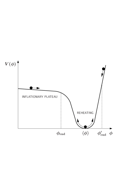
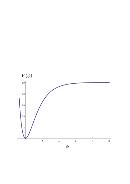
where $H$ is the rate of the Universe expansion (Hubble parameter), the dot denotes derivative with respect to the cosmic time $t$ and the prime denotes derivative with respect to the field: ${}^{\prime}\equiv\partial/\partial\phi$. The above is of the same form as the equation of motion of a ball sliding down a potential under friction determined by $H$ (see Fig. 1). Potential domination, therefore, suggests that the kinetic energy density is subdominant to the potential energy density $V$, and the field slowly rolls (slowly varies in field space) down a potential plateau, called the inflationary plateau. Inflation ends at a characteristic value $\phi_{\rm end}$ when the potential becomes steep and curved. After the end of inflation, the inflaton field oscillates around its vacuum expectation value (VEV). These coherent oscillations amount to inflaton particles, which decay into the primordial plasma, through a process called reheating.

Figure 1: Sketch of the typical inflationary potential. Due to the form of the equation of motion (1), we can envisage the system as a ball rolling down a flat region of the potential, called the inflationary plateau. At some critical value of the inflaton field $\phi_{\rm end}$, the potential becomes steep and curved such that inflation is terminated. Afterwards, the field oscillates around its vacuum expectation value $\langle\phi\rangle$. The figure also depicts the possibility that the inflaton field slow-rolls down a steep potential under excessive friction (and inflation ends when this friction is not enough for inflation at $\phi^{\prime}_{\rm end}$) but this possibility is not favoured by the observations.

Inflation however, should not make the Universe perfectly uniform, because in order for galaxies to form, initial perturbations in the density of the Universe are needed. Indeed, inflation makes the Universe largely uniform but also introduces minor deviations from uniformity which give rise to the Primordial Density Perturbations (PDPs), which in turn become the seeds for the formation of structures such as galaxies [4]. Inflation does this through the particle productions process which roughly operates as follows:

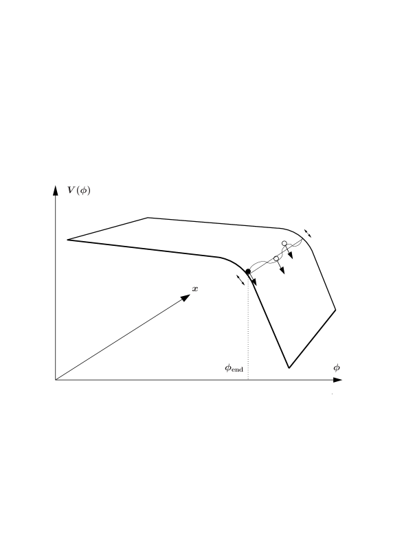
Accelerated expansion of space is superluminal. This superluminal expansion during inflation amplifies the quantum fluctuations of the inflaton field, which become classical perturbations of the field through quantum decoherence. Consequently, inflation continues a little bit more in some locations than in others. Thus, at the end of inflation space expands in a different way in neighbouring locations, which introduces the PDPs (see Fig. 2).

Figure 2: Sketch of the edge of the inflationary plateau, where inflation is terminated at the critical value $\phi_{\rm end}$. The spatial direction $x$ is also depicted (assumed one-dimensional for illustrative purposes). Perturbations of the inflaton field $\phi$ imply that, while it is rolling down its potential, it reaches the critical value $\phi_{\rm end}$ at different times at different locations (values of $x$). This means that inflation continues a little bit more in some locations than in others, which leads to the generation of the primordial density perturbations.

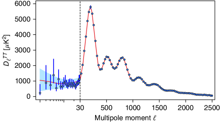
The PDP reflects itself onto the Cosmic Microwave Background radiation (CMB) through the Sachs-Wolfe effect [5]. Indeed, precise CMB observations have revealed the existence of the PDP at the level of $\sim 10^{-5}$, with the characteristics suggested by inflation (acoustic peaks). The agreement with the observations (see Fig. 3) is spectacular [6].

Figure 3: CMB temperature perturbation spectrum. The graph is a plot of ${\cal D}_{\ell}=\ell(\ell+1)C_{\ell}/2\pi$, where $C_{\ell}$ is the CMB temperature anisotropy, as a function of the multipole moment $\ell$ of spherical harmonics. For $\ell<30$ the scaling of the horizontal axis changes. The shaded area depicts the region under the influence of cosmic variance, which suggests that deviations from the theoretical curve (depicted by the solid line) within the shaded area are due to poor statistics and do not have a physical meaning. The effect of cosmic variance diminishes (virtually disappears) for large $\ell$. For $\ell\geq 30$ we have the clear depiction of seven acoustic peaks. The line between the binned data points is not the line which connects the dots; it is the theoretical line predicted by inflation. The agreement with the data is impressive. Figure taken from Ref. [6].

The PDPs are predominately adiabatic, Gaussian and scale invariant [4]. Adiabaticity suggests that they are the product of a single degree of freedom, such as the inflaton field. Gaussianity reflects the randomness of the original quantum fluctuations. Approximate scale invariance suggests that inflation is of quasi-de Sitter type, when the density $\rho$ is roughly constant during inflation. The barotropic (equation of state) parameter of a homogeneous scalar field is

$$w\equiv\frac{p}{\rho}=\frac{\frac{1}{2}\dot{\phi}^{2}-V(\phi)}{\frac{1}{2}\dot{\phi}^{2}+V(\phi)}\,,$$ (2)

where $p$ is the pressure. According to the inflationary paradigm, the kinetic energy density $\rho_{\rm kin}$ is subdominant to the potential during inflation, which means $\rho_{\rm kin}\equiv\frac{1}{2}\dot{\phi}^{2}\ll V$. As a result, during quasi-de Sitter inflation we have $w\approx-1$.

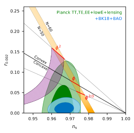
There is a lot of emphasis put on the PDP generated by inflation, because the perturbations generated can discriminate between different inflation models. In particular, two observables are of prime interest: the scalar spectral index $n_{s}$ and the tensor-to-scalar ratio $r$. For the scalar perturbations, the spectrum can be written as ${\cal P}_{\zeta}(k)\propto k^{n_{s}(k)-1}$, where $k$ is the momentum scale. A perfectly scale invariant spectrum would correspond to $n_{s}=1$, in which case all $k$-dependence of ${\cal P}_{\zeta}$ would disappear. Indeed, observations suggest that, for negligible tensor perturbations, the spectral index is very close to unity $n_{s}=0.965\pm 0.004$ [6]. Crucially, the spectral index is not exactly equal to unity because the end of inflation is near and the inflationary plateau is not exactly flat. Therefore, a slightly red spectrum is expected, exactly as observed. The tensor-to-scalar ratio is $r\equiv{\cal P}_{\zeta}/{\cal P}_{t}$, where ${\cal P}_{t}$ is the spectrum of the tensor perturbations (primordial gravitational waves). Observations suggests that there is a stringent upper limit $r<0.036$ [7], which can be even tighter under certain conditions. Precision observations of $n_{s}$ and $r$ have already resulted in the exclusion of many, otherwise well motivated inflation models (see Fig. 4).

Figure 4: Observations of BICEP/Keck Collaboration plot the tensor to scalar ratio $r$ with respect to the scalar spectral index $n_{s}$. The allowed parameter space is shown in blue (contours depict the 95% c.l. [light] and 67% c.l. [dark]). Observations exclude families of otherwise motivated inflation models. For example, the clearly excluded purple band and orange band correspond to natural and chaotic monomial inflation models respectively. The figure was taken from Ref. [7].

1.1 $R^{2}$ inflation

The seminal paper of Alexei A. Starobinsky, which appeared in 1980, even before the name ‘cosmic inflation’ was coined, introduced the very first and the most successful to date inflation model [2]. It is a modified gravity theory with a simple Lagrangian density

$${\cal L}=\frac{1}{2}m_{P}^{2}R+\alpha R^{2}\,,$$ (3)

where $m_{P}$ is the reduced Planck mass and $R$ is the scalar curvature (Ricci scalar). The first term in the above corresponds to the standard Einstein-Hilbert action. However, the second term, whose importance is parametrised by the non-perturbative coefficient $\alpha$, corresponds to modified gravity. This quadratic gravity term introduces an additional degree of freedom. The latter can be flushed out if we switch from the modified gravity frame (called the Jordan frame) to the frame of Einstein gravity (called the Einstein frame) through a conformal transformation of the spacetime metric, of the form $g_{\mu\nu}\rightarrow\Omega^{2}g_{\mu\nu}$, where the conformal factor for this theory is $\Omega^{2}=1+\frac{4\alpha}{m_{P}^{2}}R$. In the Einstein frame the Lagrangian density becomes

$${\cal L}=\frac{1}{2}m_{P}^{2}R+\frac{1}{2}(\partial\phi)^{2}-V(\phi)\,,$$ (4)

where $R$ is now calculated using the new metric and, apart from the Einstein-Hilbert term, $\cal L$ features a minimally coupled (to gravity), canonically normalised scalar field $\phi$, where $(\partial\phi)^{2}\equiv-\partial_{\mu}\phi\,\partial^{\mu}\phi$. This scalar field corresponds to the new degree of freedom introduced by the original quadratic gravity term, and it is called the scalaron field with $\Omega^{2}=\exp\left(\sqrt{\frac{2}{3}}\,\phi/m_{P}\right)$.

For this theory, in the Einstein frame, the scalar potential is

$$V(\phi)=\frac{m_{P}^{4}}{16\alpha}\left(1-e^{-\sqrt{\frac{2}{3}}\,\phi/m_{P}}\right)^{2}\,.$$ (5)

The form of the above potential is shown in Fig. 5. The model predicts

$$n_{s}=1-\frac{2}{N}\quad{\rm and}\quad r=\frac{12}{N^{2}}\,,$$ (6)

where $N$ is the number of e-folds (exponential expansions) of remaining inflation when the cosmological scales exit the horizon during inflation (they are pushed out by the superluminal expansion). Typically, $N=50-60$ depending on the details of reheating (prompt reheating results in $N=60$). The above suggest that the Starobinsky inflation predictions are in the sweet spot of the observations. For the amplitude of the PDP to match the CMB observations we require $\alpha=5.5225\times 10^{8}$.

Figure 5: Form of the Starobinsky potential, which applies to both the cases of $R^{2}$-inflation and Higgs inflation. The plot clearly depicts the inflationary plateau at large values of the inflaton field. At small values, the potential becomes steep and curved and the inflaton oscillates around its VEV, which is zero in this case. Fiducial units are used.

1.2 Higgs inflation

Another seminal inflation model was put forward by Fedor L.Bezrukov and Mikhail Shaposhnikov in 2008 [8]. The model considers the electroweak Higgs field $h$ (first observed in CERN in 2012) as the inflaton. It is another modified gravity theory with Lagrangian density

$${\cal L}=\frac{1}{2}m_{P}^{2}R+\frac{1}{2}\xi Rh^{2}+\frac{1}{2}(\partial h)^{2}-U(h)\,,$$ (7)

where $\xi$ parametrises the strength of the non-minimal coupling to gravity of the Higgs field, which is naturally introduced by quantum corrections in curved spacetime. The potential is $U(h)=\frac{1}{4}\lambda_{h}(h^{2}-v^{2})^{2}$, where $v=246\,$GeV is the Higgs VEV and $\lambda_{h}$ is its self-coupling, which at low energies is $\lambda_{h}=0.129$.

We switch to Einstein gravity using the conformal transformation $\Omega^{2}=1+\frac{\xi h^{2}}{m_{P}^{2}}$. In the Einstein frame the Lagrangian density is given by Eq. (4) with potential

$$V(\phi)=\frac{\lambda_{h}m_{P}^{4}}{4\xi^{2}}\left(1-e^{-\sqrt{\frac{2}{3}}\,\phi/m_{P}}\right)^{2}\,.$$ (8)

The above is of exactly the same form as the potential in Eq. (5) if we identify $\xi^{2}=4\alpha\lambda_{h}$. Thus, the inflationary predictions are equally successful. In fact, because the branching rations of the Higgs decays into the standard model particles are known, reheating is unambiguously defined and $N\simeq 57$. As a result, Eq. (6) suggests $n_{s}=0.965$ and $r=0.0037$, which are in excellent agreement with observations. To have the correct amplitude of the PDP we require $\xi\simeq 47000/\sqrt{\lambda_{h}}$.

2 Dark Energy

Observations suggest that the late Universe is also undergoing accelerated expansion. This is attributed to an exotic substance called dark energy, which makes up almost 70% of the Universe content at present [9]. Dark energy could correspond to a positive cosmological constant $\Lambda$ but this requires phenomenal fine-tuning (of order $10^{-120}$) which has been called ‘‘the worse fine-tuning in physics’’ (Lawrence Krauss). As a result, other proposals have been put forward. A prominent such suggestion is quintessence [10], which amounts to the fifth element after baryonic (normal) matter, dark matter, photons (mainly CMB) and neutrinos. Quintessence is a scalar field like the inflaton, typically slow-rolling down a runaway potential; a feature called the quintessential tail. Thus, the dark energy observations suggest that the Universe is undergoing a late inflation period, driven by quintessence. This late inflation is also quasi-de Sitter, with barotropic parameter $-1\leq w\leq-0.95$ [6].

Being a dynamical degree of freedom, quintessence introduces an additional requirement (compared with just $\Lambda$), that of its initial conditions. Indeed, in thawing quintessence the field is initially frozen only to unfreeze near the present time to become dominant. But the initial (frozen) value of the field must be such that the potential energy density of the field today is comparable ($\sim$ 70%) to the density of the Universe at present. This is called the coincidence requirement [9].

3 Quintessential Inflation

A promising way to overcome the coincidence requirement is the idea of quintessential inflation, proposed first by P. James E. Peebles and Alexander Vilenkin in 1999 [11]. In a nutshell, quintessential inflation is the identification of quintessence with the inflaton field.

Quintessential inflation is a natural idea, as quintessence and the inflaton are both scalar fields. It is also economic because one employs only a single degree of freedom. Furthermore, it allows to treat the physics of inflation in the early Universe and dark energy in the late Universe in a common theoretical framework, valid over a vast range of energies. Quintessential inflation has to satisfy the observations both cosmic inflation and of dark energy, which is very difficult but not impossible. Finally, the initial conditions of quintessence (the coincidence requirement) are fixed by the inflationary attractor.

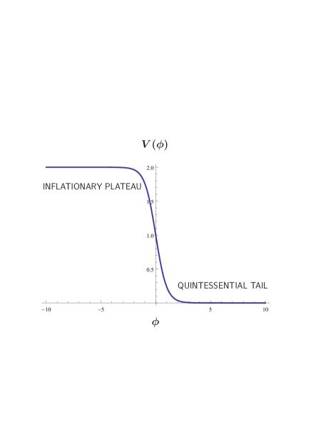
The potential of quintessential inflation models typically features two flat regions, the inflationary plateau and the quintessential tail [3] (see Fig. 6). In contrast to the traditional inflationary paradigm, the inflaton field does not decay after the end of inflation, because it has to survive until the present time and become quintessence. Consequently, reheating has to occur without the decay of the inflaton field. Fortunately, there are many motivated mechanisms that achieve this.

Figure 6: The typical potential of quintessential inflation. It depicts a runaway direction with VEV displaced at infinity. There are two flat regions, the inflationary plateau and the quintessential tail, chosen (without loss of generality) to be at small and large values of the scalar field.

3.1 Quintessential inflation in Palatini gravity

A promising framework for the construction of quintessential inflation models is modified gravity on the Palatini formalism [12]. The Palatini formalism considers both the spacetime metric and the connection to be independent degrees of freedom, in contrast to the metric formalism, where the connection is the Levi-Civita. With the Einstein-Hilbert action, both formalisms result in general relativity. However, modified gravity actions result in different theories when assuming the metric or the Palatini formalism. Here we will argue that the Palatini formalism gives rise naturally to a potential suitable for quintessential inflation.

We consider the Lagrangian density in the Jordan frame

$${\cal L}=\frac{1}{2}m_{P}^{2}R+\alpha R^{2}+\frac{1}{2}(\partial\varphi)^{2}-V(\varphi)\,,$$ (9)

where we considered a quadratic gravity term, as in Starobinsky inflation discussed in Sec. 3, and we have explicitly introduced a canonically normalised scalar field $\varphi$. We did this because, in the Palatini formalism, the quadratic gravity term $R^{2}$ does not introduce an additional degree of freedom (there is no scalaron).

Using a suitable conformal transformation, we switch to the Einstein frame, where the Lagrangian density is

$${\cal L}=\frac{1}{2}m_{P}^{2}R+\frac{\frac{1}{2}(\partial\varphi)^{2}}{1+16\alpha\frac{V(\varphi)}{m_{P}^{4}}}-\frac{V(\varphi)}{1+16\alpha\frac{V(\varphi)}{m_{P}^{4}}}\,.$$ (10)

We see that in the Einstein frame the scalar field has a non-canonical kinetic term. Notice however, that, when $V$ is very large, the unity in the denominator is negligible and the potential density approaches the constant value: $m_{P}^{4}/16\alpha$, This corresponds to the inflationary plateau, as the potential energy density does not depend of the value of the inflaton field, i.e. it is the same for a range of $\varphi$ values.

In the opposite limit, when $V$ is very small then the denominator becomes unity and the field becomes canonically normalised. Thus, we only need a suitable runaway potential to arrange for the quintessential tail, while the Palatini setup generates the inflationary plateau by ‘‘flattening’’ the potential at high energies.

We apply this finding in the following setup. Now the Lagrangian density in the Jordan frame is [13]

$${\cal L}=\frac{1}{2}m_{P}^{2}R+\alpha R^{2}+\frac{1}{2}\xi R\varphi^{2}+\frac{1}{2}(\partial\varphi)^{2}-V(\varphi)\,,$$ (11)

where we also consider a non-minimal coupling of $\varphi$ to gravity, which is expected naturally by quantum corrections in curved spacetime, as we mention in Sec. 1.2.

After performing a conformal transformation we bring the theory in the Einstein frame. We also redefine a canonically normalised inflaton field $\phi$ by using the relation

$$\left(\frac{{\rm d}\phi}{{\rm d}\varphi}\right)^{2}=\frac{1+\xi\varphi^{2}/m_{P}^{2}}{(1+\xi\varphi^{2}/m_{P}^{2})^{2}+\frac{16\alpha}{m_{P}^{4}}V(\varphi)}\,.$$ (12)

Then, the Lagrangian density becomes

$${\cal L}=\frac{1}{2}m_{P}^{2}R+\frac{1}{2}(\partial\phi)^{2}-U(\phi)\,,$$ (13)

where the potential is

$$U(\phi)=\frac{V(\varphi(\phi))}{[1+\xi\varphi^{2}(\phi)/m_{P}^{2}]^{2}+\frac{16\alpha}{m_{P}^{4}}V(\varphi(\phi))}\,.$$ (14)

We see that, again, if $V$ is very large, we approach the inflationary plateau with $U\simeq m_{P}^{4}/16\alpha$. We only need a runaway potential. We choose a simple exponential potential [13], which is amply motivated by fundamental theory:

$$V(\varphi)=V_{0}\,e^{-\kappa\varphi/m_{P}}\,,$$ (15)

where $\kappa$ is the strength of the exponential. As we approach the quintessential limit the potential of the quintessential tail approaches the form [13]

$$U(\phi)\simeq V_{0}\frac{\exp\left[-\frac{\kappa}{\sqrt{\xi}}\sinh\left(\sqrt{\xi}\frac{\phi}{m_{P}}\right)\right]}{\cosh^{4}\left(\sqrt{\xi}\frac{\phi}{m_{P}}\right)}\,,$$ (16)

where we used the fact that, at late times, the quadratic gravity term is negligible, which means that Eq. (12) can be solved exactly to give $\sqrt{\xi}\varphi=m_{P}\sinh\left(\sqrt{\xi}\phi/m_{P}\right)$. In the limit $\sqrt{\xi}\varphi\ll m_{P}$, we recover the classic exponential quintessential tail $U(\phi)\simeq V_{0}\,e^{-\kappa\phi/m_{P}}$.

4 Kination

The Universe history in quintessential inflation typically includes a period, just after inflation, where the Universe is dominated by the kinetic energy density of the rolling scalar field $\rho_{\rm kin}=\frac{1}{2}\dot{\phi}^{2}$. This period is called kination [14] and usually follows the end of inflation until reheating, when the radiation era of the hot Big Bang begins.

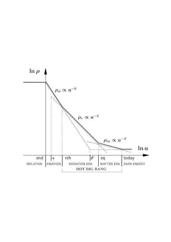
Indeed, as the inflaton rolls off the inflationary plateau, it plunges down the potential cliff (see Fig. 6) and becomes kinetically dominated, i.e. $V\ll\rho_{\rm kin}$. Because the inflaton continues to dominate the Universe, according to Eq. (2), the barotropic barotropic parameter of the Universe is $w\approx 1$. The Klein-Gordon in Eq. (1) becomes oblivious of the potential: $\ddot{\phi}+3H\dot{\phi}\simeq 0$, whose solution suggests that $\rho=\rho_{\rm kin}\propto a^{-6}$, where $a(t)$ is the scale factor of the Universe. During kination the field rolls down to the quintessential tail of its potential.

Because the energy density of radiation is diluted less efficiently with the Universe expansion, $\rho_{r}\propto a^{-4}$, if some mechanism generates some (initially subdominant) radiation at the end of inflation (or afterwards), this radiation eventually catches up with the kinetic energy density of the rolling scalar field and the Universe becomes radiation dominated. This is the moment of reheating $\rho_{\rm kin}^{\rm reh}=\rho_{r}^{\rm reh}$, the onset of the hot Big Bang.

After the radiation era begins, it can be shown that the field’s roll is impeded and soon the field freezes in some value $\phi_{F}$ (see Fig. 7). Because the roll of the scalar field is oblivious of the potential during kination and afterwards until it freezes, it can be studied in a model independent way. In particular, the total excursion of the scalar field in field space from the end of inflation and until it freezes is [15]

$$\Delta\phi_{F}=\sqrt{\frac{2}{3}}\left(2-\frac{3}{2}\ln\Omega_{r}^{\rm end}\right)\,m_{P}\;,$$ (17)

where $\Omega_{r}^{\rm end}=(\rho_{r}/\rho)_{\rm end}$ is the density parameter of radiation at the end of inflation, sometimes called reheating efficiency. Thus, we see that the smaller the reheating efficiency $\Omega_{r}^{\rm end}$ is the largest the roll of the scalar field after inflation and until it freezes and the longer the corresponding kination period is. The significance of this is discussed next.

Figure 7: Schematic log-log plot of the density of the Universe and its individual components with respect to the scale factor according to quintessential inflation. The thin solid line depicts the density of the scalar field, which is roughly constant during inflation (i.e. until inflation ends, denoted by ‘end’) and after freezing (denoted by ‘$F$’) but scales as $\rho_{\phi}\propto a^{-6}$ in between, regardless of whether it is dominant or not. The dashed line depicts the density of radiation (formed at the moment denoted by ‘$\star$’, but it is identified with ‘end’ in most cases), which scales as $\rho_{r}\propto a^{-4}$. Radiation dominates at reheating (denoted by ‘reh’), which marks the onset of the hot Big Bang. The dot-dashed line depicts the density of matter, which scales as $\rho_{m}\propto a^{-3}$ and takes over from radiation at the time of equality (denoted by ‘eq’). Today is the end of the hot Big Bang, when the density of the scalar field takes over again accounting for dark energy. The thick solid line depicts the total density.

5 Stiff Period and Gravitational Waves

In the inflationary paradigm, inflation generates an almost scale invariant superhorizon spectrum of tensor perturbations (gravitational waves) [16]. This is so only for the scales which re-enter the horizon during the radiation era of the hot Big Bang, because the density ratio $\rho_{\rm GW}/\rho$ is constant, as the energy density of the gravitational waves (GWs) scales as radiation $\rho_{\rm GW}\propto a^{-4}$ and $\rho=\rho_{r}\propto a^{-4}$ during the radiation era. However, as we have seen, during kination $\rho=\rho_{\rm kin}\propto a^{-6}$, which means that the ratio $\rho_{\rm GW}/\rho$ is not constant any more. In general, this would be true for any scales which re-enter the horizon during a period with stiff equation of state, such that $\frac{1}{3}<w\leq 1$, as $\rho\propto a^{-3(1+w)}$.

The density parameter of GWs per logarithmic frequency interval is $\Omega_{\rm GW}(f)\equiv\frac{{\rm d}\Omega_{\rm GW}}{{\rm d}\ln f}$. Then, it can be shown that the GW spectrum is of the form [17]

$$\Omega_{\rm GW}(f)\propto f^{2(\frac{3w-1}{3w+1})},$$ (18)

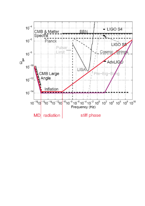
where $w$ is the barotropic parameter at the time when the scales in question re-enter the horizon. For the scales, which do so during the radiation era where $w=\frac{1}{3}$ we obtain $\Omega_{\rm GW}(f)=\,$constant, which results in a scale invariant spectrum (independent of $f$). If there is a period of kination with $w=1$, then the above suggests $\Omega_{\rm GW}\propto f$ and we have a peak in the spectrum, at the time when kination begins (usually, the end of inflation; see Fig. 7). The longer kination is the larger the peak in the GW spectrum. This peak cannot be arbitrarily large however, because too much GWs can disturb the process of Big Bang Nucleosynthesis (BBN), as we explain below.

5.1 Kination and GWs

Figure 8: Plot of the GW spectrum per logarithmic frequency interval $\Omega_{\rm GW}$ with respect to frequency, up to the largest possible frequency which corresponds to the inflation energy scale ($f_{\rm end}\sim 10^{10}\,$Hz) assumed at the scale of grand unification $\rho_{\rm end}^{1/4}\sim 10^{15-16}\,$GeV, as is typically the case. The solid purple line depicts the spectrum of primordial gravitational waves in the case of kination following right after inflation, with barotropic parameter $w=1$ and reheating temperature $T_{\rm reh}\sim 10^{2}\,$MeV. The peak in the GW spectrum almost saturates the BBN bound $\Omega_{\rm GW}<10^{-6}$, depicted by the horizontal solid black line. In the figure, the expected observational capability of Advanced LIGO [22] and LISA [21] are shown. It is evident that this scenario produces unobservable (by LISA and Advanced LIGO) primordial GW. Observational bounds have been taken from Ref. [18].

The GW energy density has to be at most 1% the the time of BBN, i.e. $\Omega_{\rm GW}^{\rm BBN}<10^{-2}$ [19]. Now, as we have said, the energy density of GWs and that of radiation stay at a constant ratio. This means that there is an upper bound on the GW energy density today, which can be computed as

$$\Omega_{\rm GW}^{0} = \frac{\rho_{\rm GW}^{0}}{\rho^{0}}\;=\;\left.\frac{\rho_{\rm GW}}{\rho_{r}}\right|_{0}\left.\frac{\rho_{r}}{\rho}\right|_{0}$$ (19)

$$= \left.\frac{\rho_{\rm GW}}{\rho_{r}}\right|_{\rm BBN}\Omega_{r}^{0}=\Omega_{\rm GW}^{\rm BBN}\,\Omega_{r}^{0}<10^{-6},$$

where we used that $\Omega_{r}^{0}=(\rho_{r}/\rho)_{0}\simeq 10^{-4}$ and that $\rho_{\rm GW}/\rho_{r}=\,$constant.

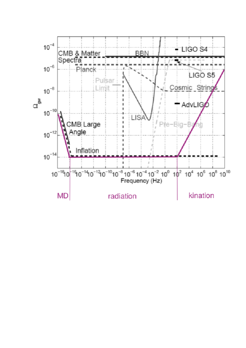
This bound means that kination cannot be arbitrary extended to late times (by considering a small reheating efficiency) because the peak in the GW spectrum would become too large and violate the bound in Eq. (19). Consequently, kination can occur only at very early times, which translates to high frequencies. A peak in the GW spectrum cannot be extended to lower frequencies and come in contact with future observations, e.g. of the LISA space interferometer. This can be understood better in Fig. 8.

5.2 GWs from a stiff period with $w\simeq\frac{1}{2}$

One way to avoid violating the bound in Eq. (19) and still extend the GW peak down to observable frequencies is to consider that, the stiff period after inflation is not as stiff as kination proper with $w=1$. Indeed, in Ref. [20] it was shown that contact with the LISA observations [21] can be achieved if $0.46\lesssim w\lesssim 0.56$ with low reheating temperature in the range 1 MeV$\,<T_{\rm reh}\lesssim\,$150 MeV. A realisation of this possibility was recently discussed in Ref. [23].

Figure 9: Qualitative form of the scalar potential in Eq. (22) in terms of the canonical scalar fields $\sigma$ (primordial inflaton) and $\phi$ (waterfall). The axes are in fiducial units. The system origitally finds itself gradually rolling down $V(\sigma)$ inside the steep valey at $\phi=0$ when $\sigma$ is large. When the inflaton is reduced below the critical value $\sigma_{c}$, a phase transition sends the waterfall field away from the origin. The minima along the canonical waterfall direction are displaced at infinity. As a result, after the phase transition, there is an initial period of fast-roll hilltop inflation along the waterfall direction, followed by a stiff period. Figure taken by Ref. [23].

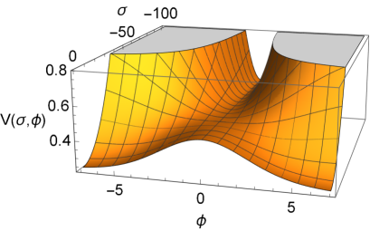
Consider two flat directions meeting at an enhanced symmetry point (ESP). The scalar potential can be written as

$$V(\varphi,\sigma)=\frac{1}{2}g^{2}\sigma^{2}\varphi^{2}+\frac{1}{4}\lambda(\varphi^{2}-M^{2})^{2}+V(\sigma)\,,$$ (20)

where the strength of the interaction is parametrised by the perturbative coupling constant $g<1$ (we assume that the ESP is at the origin), $\lambda$ is the self-coupling of the $\varphi$-field, whose VEV is $M$ and $V(\sigma)$ is the potential along the $\sigma$-direction. As we discuss below, $M\sim m_{P}$, so $\varphi$ is a flat direction lifted by Planck-suppressed operators. The above potential in Eq. (20) is the standard perturbative potential in hybrid inflation [24], where $\sigma$ plays the role of the primordial inflaton field. As in standard hybrid inflation, during primordial inflation the interaction term sends the waterfall field $\varphi$ to zero, while $V(\sigma)$ provides a gentle slope which allows the inflaton to slow-roll towards the origin. Primordial inflation is terminated by a phase transition, when $\sigma=\sigma_{c}\equiv\sqrt{\lambda}\,M/g$ and the waterfall field is released from the origin towards its VEV.

Figure 10: Plot of the GW spectrum per logarithmic frequency interval $\Omega_{\rm GW}$ with respect to frequency, up to the largest possible frequency which corresponds to the inflation energy scale ($f_{\rm end}\sim 10^{10}\,$Hz) assumed at the scale of grand unification $\rho_{\rm end}^{1/4}\sim 10^{15-16}\,$GeV, as is typically the case. The solid purple line depicts the spectrum of primordial GWs in the case of kination following right after inflation, with barotropic parameter $w=1$, while the solid red line depicts the spectrum of primordial GWs in the stiff barotropic parameter $w=\frac{1}{2}$ scenario, with reheating temperature $T_{\rm reh}\sim 10^{2}\,$MeV. The peak in the GW spectrum almost saturates the BBN bound $\Omega_{\rm GW}<10^{-6}$, depicted by the horizontal solid black line. In the figure, the expected observational capability of Advanced LIGO and LISA are shown. It is evident that this scenario produces marginally observable (by LISA and Advanced LIGO) primordial GWs. Observational bounds have been taken from Ref. [18].

This is when things become different, because we assume there is a kinetic pole at the VEV of the waterfall field. Such a pole can be due to some non-trivial Kähler geometry as with $\alpha$-attractors [25]. The Lagrangian density is

$${\cal L}=\frac{1}{2}(\partial\sigma)^{2}+\frac{\frac{1}{2}(\partial\varphi)^{2}}{(1-\varphi^{2}/M^{2})^{2}}-V(\varphi,\sigma)\,.$$ (21)

To assist our intuition we redefine the waterfall field so that it also is characterised by a canonical kinetic term. The redefinition is $\varphi=M\tanh(\phi/M)$, and $\phi$ is now canonically normalised. The scalar potential now becomes

$$V(\phi,\sigma)=\frac{1}{2}g^{2}M^{2}\sigma^{2}\tanh^{2}(\phi/M)+\frac{\frac{1}{4}\lambda M^{4}}{\cosh^{4}(\phi/M)}+V(\sigma)\,.$$ (22)

The form of the above potential is shown in Fig. 9.

After the phase transition which ends primordial inflation, $\sigma$ quickly goes to zero and the system rolls along the runaway waterfall direction, since the VEV of $\phi$ is at infinity. Now, exactly because $M$ is Planckian, we have a further boot of fast-roll inflation [26] as the waterfall field leaves the origin, which is now a potential hill

$$V(\phi\ll M)\simeq\frac{\frac{1}{4}\lambda M^{4}}{[1+\frac{1}{2}(\phi/M)^{2}]^{4}}\simeq\frac{1}{4}\lambda M^{4}\left[1-2\left(\frac{\phi}{M}\right)^{2}\right].$$ (23)

Based on the value of $M$, this gives about 13.5 e-folds of hilltop fast-roll inflation, following the primordial inflation. Inflation ends when $\phi_{\rm end}\simeq M/\sqrt{2}$. Afterwards, the canonical waterfall rolls along the potential tail with

$$V(\phi\gg M)\simeq\frac{\frac{1}{4}\lambda M^{4}}{[\frac{1}{2}\exp(\phi/M)]^{4}}\simeq 4\lambda Me^{-4\phi/M}.$$ (24)

Since the potential tail is of exponential form, the field soon follows the power-law inflation attractor [27] which is characterised by the barotropic parameter $w=-1+\frac{16}{3}\left(\frac{m_{P}}{M}\right)^{2}.$ Requiring $w\approx\frac{1}{2}$ suggests that $M/m_{P}\approx\frac{4\sqrt{2}}{3}=1.88$. This is why we considered that $M\sim m_{P}$ in the first place.

As can be seen in Fig. 10, the peak in the GW spectrum is much more mild and it can come to contact with the future LISA observations.

5.3 Hyperkination and GWs

Another possibility to boost the primordial GWs generated during inflation at observable frequencies is by considering the model of Sec. 3.1, which is characterised by the Lagrangian density in Eq. (11). Switching to Einstein frame through a suitable conformal transformation, the Lagrangian density becomes

$${\cal L}=\frac{1}{2}m_{P}^{2}R+\frac{1}{2}(\partial\phi)^{2}+\alpha\frac{h^{2}+16\alpha V}{h^{2}m_{P}^{4}}(\partial\phi)^{4}-\frac{Vm_{P}^{4}}{h^{2}+16\alpha V}\,,$$ (25)

where $h^{2}\equiv m_{P}^{2}+\xi\varphi^{2}$, with $\varphi$ being the non-canonical field, which appears in Eq. (11). Then, the Klein-Gordon equation of motion of the field is

$$\left[1+12\alpha\left(1+\frac{16\alpha V}{h^{2}}\right)\right]\ddot{\phi}\;+$$

$$\left[1+4\alpha\left(1+\frac{16\alpha V}{h^{2}}\right)\frac{\dot{\phi}^{2}}{m_{P}^{4}}\right]3H\dot{\phi}\;+$$

$$48\alpha^{2}\frac{\dot{\phi}^{4}}{m_{P}^{4}}\frac{\rm d}{\rm d\phi}\left(\frac{V}{h^{2}}\right)+\frac{\rm d}{\rm d\phi}\frac{Vm_{P}^{4}}{h^{2}+16\alpha V} = 0\,.$$ (26)

From the energy-momentum tensor, it is straightforward to obtain the energy density and the pressure of the scalar field, which respectively read

$$\rho_{\phi} = \frac{1}{2}\left[1+6\alpha\left(1+\frac{16\alpha V}{h^{2}}\right)\frac{\dot{\phi}^{2}}{m_{P}^{4}}\right]\dot{\phi}^{2}+\frac{Vm_{P}^{4}}{h^{2}+16\alpha V}\,,$$

$$p_{\phi} = \frac{1}{2}\left[1+2\alpha\left(1+\frac{16\alpha V}{h^{2}}\right)\frac{\dot{\phi}^{2}}{m_{P}^{4}}\right]\dot{\phi}^{2}-\frac{Vm_{P}^{4}}{h^{2}+16\alpha V}\,.$$

Figure 11: Plot of the GW spectrum per logarithmic frequency interval $\Omega_{\rm GW}$ with respect to frequency, up to the largest possible frequency which corresponds to the inflation energy scale ($f_{\rm end}\sim 10^{10}\,$Hz) assumed at the scale of grand unification $\rho_{\rm end}^{1/4}\sim 10^{15-16}\,$GeV, as is typically the case. The solid purple line depicts the spectrum of primordial GWs in the case of kination following right after inflation, with barotropic parameter $w=1$, while the solid red line depicts the spectrum of primordial GWs in the stiff barotropic parameter $w=\frac{1}{2}$ scenario and the solid green line depicts the spectrum of primordial GWs in the case when inflation is followed first by a period of hyperkination and then by a period of regular kination, with reheating temperature $T_{\rm reh}\sim 10^{2}\,$MeV. This time, the spectrum of the GWs is nowhere near the BBN bound $\Omega_{\rm GW}<10^{-6}$, depicted by the horizontal solid black line. In the figure, the expected observational capability of Advanced LIGO and LISA are shown. It is evident that this scenario produces a distinct, characteristic spectrum of observable (by LISA and Advanced LIGO) primordial GWs. Observational bounds have been taken from Ref. [18].

The above complicated expressions are much simplified if, after the end of inflation, the scalar field becomes kinetically dominated. In this case, we can set $V\rightarrow 0$ so that Eqs. (26) and (LABEL:rhop0) are respectively reduced to

$$\left(1+12\alpha\frac{\dot{\phi}^{2}}{m_{P}^{4}}\right)\ddot{\phi}+\left(1+4\alpha\frac{\dot{\phi}^{2}}{m_{P}^{4}}\right)3H\dot{\phi}\simeq 0$$ (28)

and

$$\rho_{\phi} \simeq \frac{1}{2}\left(1+6\alpha\frac{\dot{\phi}^{2}}{m_{P}^{4}}\right)\dot{\phi}^{2},$$

$$p_{\phi} \simeq \frac{1}{2}\left(1+2\alpha\frac{\dot{\phi}^{2}}{m_{P}^{4}}\right)\dot{\phi}^{2}.$$

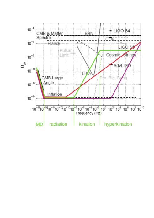
Now, if the standard quadratic kinetic term is dominant in Eq. (25), then this is equivalent to setting $\alpha\rightarrow 0$. In this case, Eq. (LABEL:rhop) suggests that $w_{\phi}=p_{\phi}/\rho_{\phi}=1$ and we have regular kination, which results in $\Omega_{\rm GW}(f)\propto f$ as we have discussed. If however, the quartic kinetic term is dominant in Eq. (25), then this is equivalent to considering only the terms proportional to $\alpha$. In this case, Eq. (LABEL:rhop) suggests that $w_{\phi}=p_{\phi}/\rho_{\phi}=\frac{1}{3}$, similarly to radiation, for which $\Omega_{\rm GW}(f)=\,$constant. We call this period hyperkination [28].

Because, after inflation, the quartic kinetic term dominates before the quadratic one takes over (and not the other way around), after inflation we have a period of hyperkination followed by a period of regular kination until reheating. This results in a GW spectrum, which features a truncated peak such that boosting the primordial GWs can occur at lower observable frequencies without violating the BBN bound in Eq. (19). The situation is depicted in Fig. 11. The distinct GW spectrum, if observed, could provide information on the theoretical background, such as the energy scale of inflation and the value of the $\alpha$ parameter, which characterises the contribution of the quadratic gravity, as shown in Eq. (11).

6 Conclusions

Cosmic Inflation determines the initial conditions of the Universe history and leads to a large and uniform Universe. Inflation also generates the primordial density perturbations which seed galaxy formation and are reflected on the CMB primordial anisotropy. Agreement between the CMB observations and the predictions of inflation is spectacular. In addition, the Universe today engages into a late inflationary period, which may be due to quintessence, a form of dark energy.

Quintessential inflation employs a common theoretical framework for the early and late Universe and leads to a surge in primordial gravitational waves. Typically, quintessential inflation is modelled considering a flat direction with a runaway scalar potential, which has minimum at infinity and features two flat regions: the inflationary plateau and the quintessential tail. Palatini gravity is a natural framework for model-building quintessential inflation because it ‘‘flattens’’ a runaway potential to generate the inflationary plateau.

Quintessential inflation is typically followed by a stiff period called kination, which generated a peak of primordial gravitational waves (GWs). However, the kination GW peak corresponds to unobservable frequencies. One way to overcome this is by considering that the peak is milder, which can be achieved in the stiff period after inflation is not as stiff as kination proper. A model realisation of this possibility considers two flat directions intersecting at an enhanced symmetry point in field space, giving rise to the hybrid mechanism, with Planckian waterfall field VEV, which is also a kinetic pole of the waterfall field, following the $\alpha$-attractors proposal.

Another interesting possibility to obtain a boost of primordial GWs down at observable frequencies in by considering higher order kinetic terms (as in k-essence [29]). This is possible to realise in Palatini modified gravity. Indeed, considering $R+R^{2}$ gravity and a non-minimally coupled scalar field gives rise to additional quartic kinetic terms. When these dominate, this leads to hyperkination which is followed by regular kination when the field becomes canonical. the resulting characteristic truncated GW peak can be extended to observable frequencies without disturbing BBN.

Forthcoming observations of Advanced LIGO, LISA, DesiGO or BBO may well detect the primordial GWs generated by inflation. A distinct GW spectrum will provide insights to the background theory. Finally, it should be pointed out that the detection of primordial GWs will not only confirm another prediction of cosmic inflation but also offer tantalising evidence for the quantum nature of gravity itself.

References

- [1] A. H. Guth, Phys. Rev. D 23 (1981), 347-356.
- [2] A. A. Starobinsky, Phys. Lett. B 91 (1980), 99-102.
- [3] K. Dimopoulos, Introduction to Cosmic Inflation and Dark Energy, CRC Press, 2022, ISBN 978-0-367-61104-0
- [4] D. H. Lyth and A. R. Liddle, The primordial density perturbation: Cosmology, inflation and the origin of structure, CUP, 2009, ISBN 978-0521828499
- [5] R. K. Sachs and A. M. Wolfe, Astrophys. J. 147 (1967), 73-90.
- [6] P. A. R. Ade et al. [Planck], Astron. Astrophys. 594 (2016), A20.
- [7] P. A. R. Ade et al. [BICEP and Keck], Phys. Rev. Lett. 127 (2021) no.15, 151301.
- [8] F. Bezrukov, A. Magnin, M. Shaposhnikov and S. Sibiryakov, JHEP 01 (2011), 016.
- [9] A. G. Riess et al. [Supernova Search Team], Astron. J. 116 (1998), 1009-1038; S. Perlmutter et al. [Supernova Cosmology Project], Astrophys. J. 517 (1999), 565-586.
- [10] R. R. Caldwell, R. Dave and P. J. Steinhardt, Phys. Rev. Lett. 80 (1998), 1582-1585; S. M. Carroll, Phys. Rev. Lett. 81 (1998), 3067-3070.
- [11] P. J. E. Peebles and A. Vilenkin, Phys. Rev. D 59 (1999), 063505.
- [12] K. Dimopoulos and S. Sánchez López, Phys. Rev. D 103 (2021) no.4, 043533.
- [13] K. Dimopoulos, A. Karam, S. Sánchez López and E. Tomberg, Galaxies 10 (2022) no.2, 57; JCAP 10 (2022), 076.
- [14] M. Joyce and T. Prokopec, Phys. Rev. D 57 (1998), 6022-6049.
- [15] K. Dimopoulos and C. Owen, JCAP 06 (2017), 027.
- [16] M. S. Turner, Phys. Rev. D 55 (1997), R435-R439.
- [17] Y. Gouttenoire, G. Servant and P. Simakachorn, [arXiv:2111.01150 [hep-ph]].
- [18] E. Thrane and J. D. Romano, Phys. Rev. D 88 (2013) no.12, 124032.
- [19] R. H. Cyburt, B. D. Fields, K. A. Olive and E. Skillman, Astropart. Phys. 23 (2005), 313-323.
- [20] D. G. Figueroa and E. H. Tanin, JCAP 08 (2019), 011.
- [21] P. Amaro-Seoane et al. [LISA], [arXiv:1702.00786 [astro-ph.IM]].
- [22] J. Aasi et al. [LIGO Scientific], Class. Quant. Grav. 32 (2015), 074001.
- [23] K. Dimopoulos, JCAP 10 (2022), 027.
- [24] A. D. Linde, Phys. Rev. D 49 (1994), 748-754.
- [25] R. Kallosh, A. Linde and D. Roest, JHEP 11 (2013), 198.
- [26] A. D. Linde, JHEP 11 (2001), 052.
- [27] F. Lucchin and S. Matarrese, Phys. Rev. D 32 (1985), 1316.
- [28] S. Sánchez López, K. Dimopoulos, A. Karam and E. Tomberg, Eur. Phys. J. C 83 (2023) no.12, 1152.
- [29] C. Armendariz-Picon, V. F. Mukhanov and P. J. Steinhardt, Phys. Rev. Lett. 85 (2000), 4438-4441; Phys. Rev. D 63 (2001), 103510.