Santaló Geometry of Convex Polytopes

Abstract

The Santaló point of a convex polytope is the interior point which leads to a polar dual of minimal volume. This minimization problem is relevant in interior point methods for convex optimization, where the logarithm of the dual volume is known as the universal barrier function. When translating the facet hyperplanes, the Santaló point traces out a semi-algebraic set. We describe and compute this geometry using algebraic and numerical techniques. We exploit connections with statistics, optimization and physics.

1 Introduction

This article studies the (semi-)algebraic geometry of minimizing volumes of dual polytopes. Motivations include optimization, statistics and particle physics. To make this more precise, we start with some terminology. A polytope $P\subset\mathbb{R}^{m}$ is the convex hull of finitely many points. If $P$ has dimension $m$, then each point $y$ in its interior defines a dual polytope

$$(P-y)^{\circ}\,=\,\{z\in(\mathbb{R}^{m})^{\vee}\,:\,\langle y^{\prime}-y,z\rangle\leq 1,\,\,\text{for all}\,\,y^{\prime}\in P\}.$$

The function $y\mapsto{\rm vol}_{m}\,(P-y)^{\circ}$ is strictly convex on the interior of $P$. In fact, this is true when $P$ is replaced by any convex body, see the proof of Proposition 1(i) in [27]. It follows that there is a unique minimizer $y^{*}\in{\rm int}(P)$. That point is called the Santaló point of $P$:

$$y^{*}\,=\,\underset{y\in{\rm int}(P)}{\operatorname{argmin}}\,\,{\rm vol}_{m}\,(P-y)^{\circ}\,=\,\underset{y\in{\rm int}(P)}{\operatorname{argmin}}\,\,\int_{(P-y)^{\circ}}{\rm d}z_{1}\cdots{\rm d}z_{m}.$$ (1)

A special property of polytopes, compared to general convex bodies, is that our volume function is rational. It follows from Theorems 3.1 and 3.2 in [13] that

$${\rm vol}_{m}\,(P-y)^{\circ}\,=\,\gamma\cdot\frac{\alpha_{P}(y)}{\ell_{1}(y)\cdot\cdots\cdot\ell_{k}(y)},$$ (2)

where $\gamma$ is a nonzero real constant, $\ell_{i}(y)=0$ is an affine-linear equation defining the $i$-th facet hyperplane of $P$, and $\alpha_{P}(y)$ is the adjoint polynomial. We will recall a formula for $\alpha_{P}$ in Section 2. Having established the identity (2), computing the Santaló point of $P$ comes down to minimizing a convex rational function or, equivalently, its logarithm.

Example 1.1 ($m=2,k=5$).

We consider the pentagon $P$ in $\mathbb{R}^{2}$ given by the inequalities

$$y_{1}+\frac{1}{5}\geq 0,\quad y_{2}+\frac{1}{5}\geq 0,\quad 2y_{1}+2y_{2}+\frac{1}{5}\geq 0,\quad-2y_{1}-y_{2}+\frac{1}{5}\geq 0,\quad-y_{1}-2y_{2}+\frac{1}{5}\geq 0.$$

It is shown, together with the poles and zeros of ${\rm vol}_{2}(P-y)^{\circ}$, in Figure 1 (left). We have

$${\rm vol}_{2}(P-y)^{\circ}\,=\,\frac{1}{125}\dfrac{-50y_{1}^{2}-25y_{1}y_{2}+15y_{1}-50y_{2}^{2}+15y_{2}+11}{(y_{1}+\frac{1}{5})(y_{2}+\frac{1}{5})(2y_{1}+2y_{2}+\frac{1}{5})(-2y_{1}-y_{2}+\frac{1}{5})(-y_{1}-2y_{2}+\frac{1}{5})}.$$ (3)

The Santaló point minimizes this function on ${\rm int}(P)$: ${y^{*}=(-0{.}00311069,-0{.}00311069)}$.

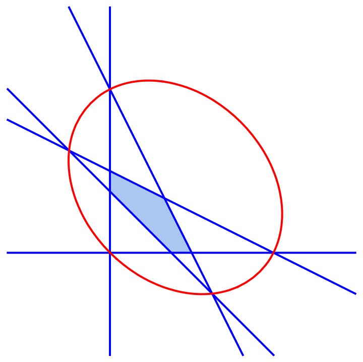
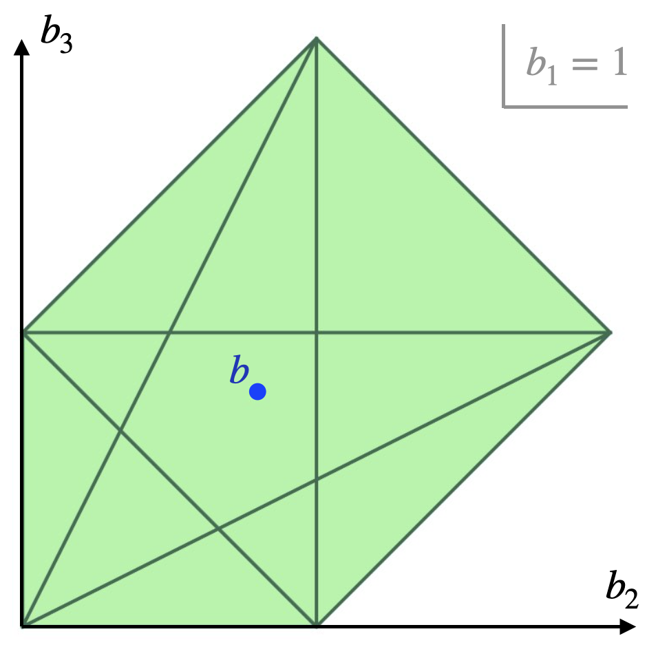
Figure 1: Left: the pentagon $P$ from Example 1.1, together with its adjoint curve (red) and facet hyperplanes (blue). Right: a two-dimensional slice of the chamber complex ${\cal C}_{A}$.

The first motivation for computing Santaló points comes from convex optimization [29]. In that context, $P$ is the feasible region of a linear program, whose optimal solution is typically a vertex of $P$. Interior point methods approximate that vertex by first optimizing a strictly convex (barrier) function. The resulting interior optimizer is then tracked to the optimal vertex by varying a regularization parameter. For more details, see [16, 29], where (2) is called the universal barrier. For a summary, see the introduction of [34].

We are interested in how the Santaló point varies when the facet hyperplanes of $P$ are translated. More precisely, we fix a nonnegative $(d\times n)$-matrix $A\in\mathbb{R}^{d\times n}_{\geq 0}$ of rank $d$, none of whose columns is the zero vector, and consider the fibers of the projection $A:\mathbb{R}^{n}_{\geq 0}\rightarrow\mathbb{R}^{d}$:

$$P_{b}\,=\,\{x\in\mathbb{R}^{n}_{\geq 0}\,:\,Ax=b\},\quad b\in{\rm pos}(A).$$

Here ${\rm pos}(A)$ is the image of $A:\mathbb{R}^{n}_{>0}\rightarrow\mathbb{R}^{d}$. If $b$ lies in ${\rm pos}(A)$, then $P_{b}$ is a polytope of dimension $m=n-d$. A point $x$ in its relative interior defines a full-dimensional polytope $P_{b}-x$ in the $(n-d)$-dimensional vector space $\ker A\simeq\mathbb{R}^{n-d}$. We define

$$V\,:\,\mathbb{R}^{n}_{>0}\,\longrightarrow\,\mathbb{R}_{\geq 0},\quad x\,\longmapsto\,{\rm vol}_{n-d}\,(P_{Ax}-x)^{\circ}.$$ (4)

This is defined up to a scaling factor, which depends on the choice of basis for $\ker A$. We prove that this global volume function is piecewise rational, meaning that it is a rational function when restricted to certain $n$-dimensional subcones of $\mathbb{R}^{n}_{>0}$ (Proposition 2.7). These subcones correspond to the cells of the chamber complex $\mathcal{C}_{A}$ associated to $A$, see for instance [5]. Moreover, on each of these subcones, $V$ is homogeneous of degree $d-n$ (Proposition 2.7).

Each fiber $P_{b}$ has a unique Santaló point. This defines a natural section of $A:\mathbb{R}^{n}_{>0}\rightarrow\mathbb{R}^{d}$:

$$x^{*}(b)\,=\,\underset{x\in{\rm int}(P_{b})}{\operatorname{argmin}}\,\,V(x)\,.$$ (5)

The map $x^{*}:{\rm pos}(A)\rightarrow\mathbb{R}^{n}_{>0}$ is piecewise algebraic. Its image is called the Santaló patchwork. We show that the Santaló patchwork is a union of $d$-dimensional basic semi-algebraic sets, one for each $d$-dimensional cell in the chamber complex ${\cal C}_{A}$ (Corollary 3.4). We give inequalities for each of its pieces (called Santaló patches), and bound the degree of their Zariski closures.

Example 1.2 ($d=3,n=5$).

The pentagon in Example 1.1 is the fiber $P_{b}-x$ for the data

$$A\,=\,\begin{pmatrix}1&1&1&1&1\\ 2&1&0&1&0\\ 1&2&0&0&1\end{pmatrix},\quad\quad b\,=\,\frac{1}{5}\begin{pmatrix}5\\ 4\\ 4\end{pmatrix},\quad x=\frac{1}{5}\begin{pmatrix}1&1&1&1&1\end{pmatrix}^{T}.$$ (6)

The coordinates $y_{1}$ and $y_{2}$ in Example 1.1 are with respect to the following basis of $\ker A$:

$$B\,=\,\frac{1}{18}\begin{pmatrix}5&-4&2&-6&3\\ -4&5&2&3&-6\end{pmatrix}^{T}.$$

The columns of $A$ are the vertices of a pentagon in $\mathbb{R}^{3}$. They define the polyhedral complex shown in Figure 1 (right). The Chamber complex ${\cal C}_{A}$ is the polyhedral fan over that complex. There are 11 $3$-dimensional cells. Our $b$ lies in the central pentagonal cell. For any $x\in\mathbb{R}^{5}_{\geq 0}$ such that $Ax$ lies in this cell, we have the following formula for the volume function $V(x)$:

$$V(x)\,=\,\frac{3x_{1}x_{2}x_{3}+2x_{1}x_{3}x_{5}+2x_{1}x_{4}x_{5}+2x_{2}x_{3}x_{4}+2x_{2}x_{4}x_{5}}{x_{1}x_{2}x_{3}x_{4}x_{5}}.$$ (7)

To match this with (3), use $Ax=b$ and $B^{T}x=y$ to switch from $x$- to $(b,y)$-coordinates and substitute $b=(1,4/5,4/5)$. A different rational function is needed when $b$ belongs to a different cell, because the combinatorial type of $P_{b}$ changes. For instance, one checks that for $b=(1,6/5,4/5)$, $P_{b}$ is a quadrilateral. Each cell in ${\cal C}_{A}$ gives a patch of the Santaló patchwork, which is a 3-dimensional semi-algebraic set in $\mathbb{R}^{5}_{\geq 0}$. Intersecting this with the 4-dimensional simplex $\{\sum_{i=1}^{5}x_{i}=1\}$ and projecting to $\mathbb{R}^{3}$, we obtain Figure 2.

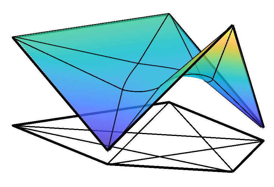
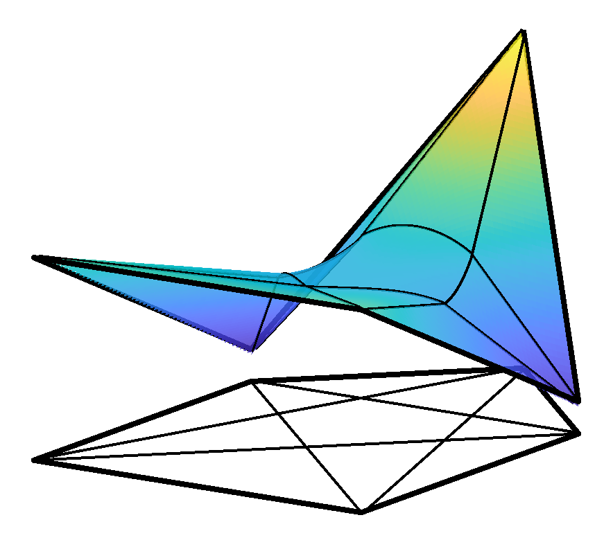
Figure 2: Visualization of the Santaló patchwork for $A$ from (6).

Understanding the degrees of Santaló patches relies on insights from algebraic statistics [11]. Minimizing the logarithm of the dual volume has the interpretation of maximum likelihood estimation for a particular discrete statistical model, called Wachspress model [24, Section 2]. Every righthand side vector $b\in{\rm pos}(A)$ defines a Wachspress model. The maximum likelihood degree (ML degree) [8] of this model is constant for generic $b$ in the interior of a cell in the chamber complex. We conjecture that, under mild genericity assumptions, it gives a lower bound for the degree of the corresponding Santaló patch, see Conjecture 4.10 and Proposition 5.7. Example 5.14 gives evidence for the claim that this lower bound is close to the actual degree of the Santaló patch. We show how to compute the ML degree numerically, and Conjecture 5.12 gives a formula for polygons. A sketch of proof is also included.

Our outline is as follows. Section 2 studies the volume function (4). Sections 3 and 4 describe the Santaló patchwork and its Zariski closure. Section 5 makes the link to Wachspress models. Finally, In Section 6 we discuss homotopy based methods for computing Santaló points. First, we use monodromy to compute the Santaló point of some fiber $P_{b_{0}}$. Next, we compute the Santaló point of a new fiber $P_{b_{1}}$ from that of $P_{b_{0}}$, such that $b_{0}$ and $b_{1}$ belong to the same chamber of ${\cal C}_{A}$. We use numerical homotopy continuation [33] to track $x^{*}(b_{0})$ to $x^{*}(b_{1})$ along a smooth path on the Santaló patchwork. Our algorithms are implemented in a Julia package Santalo.jl, which is available at https://mathrepo.mis.mpg.de/Santalo.

Our work fits nicely into a broader story of semi-algebraic sets in convex optimization, algebraic statistics and particle physics. Different strictly convex objective functions used in interior point methods give rise to other interesting geometric objects, see [10, 34]. For the log-barrier function $V(x)=-\sum_{i=1}^{n}\log x_{i}$, the role of the Santaló patchwork is played by the positive reciprocal linear space associated to the row span of the matrix $A$. The Santaló point is replaced by the analytic center. Entropic regularization uses $V(x)=\sum_{i=1}^{n}x_{i}\log x_{i}-x_{i}$ and leads naturally to consider the positive toric $d$-fold associated to $A$, with the Birch point being its unique intersection with $P_{b}$. From a statistical point of view, these scenarios correspond to maximum likelihood estimation for linear models and exponential families respectively. Next to optimization and statistics, the dual volume function (2) shows up in particle physics as the canonical function of $P$, viewed as a positive geometry [3]. This enters in the proof of Propostion 2.7. For some specific polytopes, $V(x)$ is a scattering amplitude [2]. Recently, dual volumes have been used in the study of toric singularities [28].

All of these connections motivate our effort to study the Santaló geometry of polytopes. Our work provides new theoretical insights into Santaló points, and practical tools for computing them. It leads to several new possible research directions, as summarized in Section 6.

2 Dual volumes of polytopes

To avoid confusion, below we write $Q\subset\mathbb{R}^{m}$ for a full-dimensional polytope (where, usually, $m=n-d$), and $P_{b}\subset\mathbb{R}^{n}$ for the $(n-d)$-dimensional fibers of $A:\mathbb{R}^{n}_{\geq 0}\rightarrow{\rm pos}(A)$.

This section describes the dual volume function (2) of a full-dimensional polytope $Q\subset\mathbb{R}^{m}$. We start with the numerator of this rational function, called the adjoint polynomial $\alpha_{Q}(y)$. We say that $Q$ is simple if each vertex is adjacent to exactly $m$ facets.

Suppose $Q$ is simple and has minimal facet representation

$$Q=\{y^{\prime}\in\mathbb{R}^{m}\,:\,\langle w_{i},y^{\prime}\rangle+c_{i}\geq 0,\,i=1,\ldots,k\}.$$ (8)

Here $w_{i}\in\mathbb{R}^{m}$ and $c_{i}\in\mathbb{R}$. The adjoint polynomial of $Q$, introduced by Warren [36], is

$$\alpha_{Q}(y)\,=\,\mathrm{vol}_{m}(Q-y)^{\circ}\cdot\prod\limits_{i=1}^{k}(\langle w_{i},y\rangle+c_{i}).$$ (9)

For completeness, we include a proof of a convenient formula for $\alpha_{Q}(y)$. We collect the vectors $w_{i}$ in an $m\times k$ matrix $W$ and write $W_{I}$ for the submatrix of columns indexed by $I\subset\{1,\ldots,k\}$. Let ${\cal V}(Q)$ be the set of vertices of $Q$. For each $v\in\mathcal{V}(Q)$, we let $I(v)=\{i\,:\,\langle w_{i},v\rangle+c_{i}=0\}\subset\{1,\ldots,k\}$ be the $m$-element index set of the facets containing $v$.

Proposition 2.1.

For a simple full-dimensional polytope $Q\subset\mathbb{R}^{m}$ with minimal facet representation (8) the adjoint polynomial $\alpha_{Q}(y)$ is given by

$$\alpha_{Q}(y)\,=\,\sum\limits_{v\in\mathcal{V}(Q)}|\det W_{I(v)}|\cdot\prod\limits_{i\not\in I(v)}\left(\langle w_{i},y\rangle+c_{i}\right).$$ (10)

Proof 2.2.

For $y\in\mathrm{int}(Q)$ the translated polytope $Q-y$ has the following facet representation:

$$Q-y\,=\,\{y^{\prime}\in\mathbb{R}^{m}\,:\,\langle w_{i},y^{\prime}\rangle+(\langle w_{i},y\rangle+c_{i})\geq 0,\,i=1,\ldots,k\}.$$

The dual polytope is then simplicial and can be described as

$$(Q-y)^{\circ}\,=\,\mathrm{conv}\left(\left\{\dfrac{w_{i}}{\langle w_{i},y\rangle+c_{i}},\,i=1,\ldots,k\right\}\right).$$

We compute its volume as the sum of volumes over pieces of its triangulation:

$$\mathrm{vol}_{m}(Q-y)^{\circ}=\sum\limits_{v\in\mathcal{V}(Q)}\mathrm{vol}_{m}\left(\mathrm{conv}\left(\{0\}\cup\bigcup\limits_{i\in I(v)}\left\{\dfrac{w_{i}}{\langle w_{i},y\rangle+c_{i}}\right\}\right)\right)=\\ \sum\limits_{v\in\mathcal{V}(Q)}\left|\det W_{I(v)}\right|\prod_{i\in I(v)}\left(\langle w_{i},y\rangle+c_{i}\right)^{-1}.$$

Since by definition $\alpha_{Q}(y)=\mathrm{vol}_{m}(Q-y)^{\circ}\cdot\prod\limits_{i=1}^{k}(\langle w_{i},y\rangle+c_{i})$, we get the formula in (10).

To avoid confusion, we point out that what we call the adjoint of $Q$ is the adjoint of the dual polytope $Q^{\circ}$ in some of the literature [23, 36]. The variety inside $\mathbb{R}^{m}$ defined by $\alpha_{Q}$ is the adjoint hypersurface associated to $Q$, see [23]. When the facet hyperplanes of $Q$ form a simple arrangement (that is, the intersection of any $i$ hyperplanes has codimension $i$), the adjoint hypersurface is the unique hypersurface of minimal degree interpolating the residual arrangement of $Q$. This arrangement is the union of all affine spaces that are contained in the intersections of facet hyperplanes but do not contain a face of $Q$ [23, Theorem 6]. In Figure 1 (left), the residual arrangement consists of 5 points defining a unique adjoint conic.

We now switch to the setting of the introduction, where $m=n-d$ and the polytope $Q$ arises as a fiber $P_{b}$ of the linear projection $A:\mathbb{R}^{n}_{\geq 0}\rightarrow\mathbb{R}^{d}$ for some $A\in\mathbb{R}^{d\times n}_{\geq 0}$. If $x$ is an interior point of $P_{b}$, then the translate $P_{b}-x$ is a full-dimensional polytope inside $\ker A\cong\mathbb{R}^{n-d}$. We are interested in minimizing its dual volume $\mathrm{vol}_{n-d}(P_{b}-x)^{\circ}$ with respect to $x$. In order to treat this problem algebraically, we will first project $P_{b}$ to $\ker A$. To do so, fix an $(n\times(n-d))$-matrix $B$ whose columns span $\ker A$. The projection of $P_{b}$ is denoted by $Q_{b}=B^{T}\cdot P_{b}$ and the coordinates $y$ on $\ker A$ are induced from $y=B^{T}x$.

By construction, the matrix obtained by concatenating $A$ and $B^{T}$ vertically is an $n\times n$ matrix of full rank. It therefore defines an invertible coordinate change

$$\begin{pmatrix}b\\ y\end{pmatrix}\,=\,\begin{pmatrix}A\\ B^{T}\end{pmatrix}x.$$ (11)

This means that in order to compute the Santaló point $x^{*}(b)$ of $P_{b}$, it is sufficient to compute the Santaló point $y^{*}(b)$ of $Q_{b}$ and then apply the inverse coordinate change:

$$x^{*}(b)=\begin{pmatrix}A\\ B^{T}\end{pmatrix}^{-1}\begin{pmatrix}b\\ y^{*}(b)\end{pmatrix}.$$ (12)

We will now study the dual volume function ${\rm vol}_{n-d}\,(Q_{b}-y)^{\circ}$ for the polytope $Q_{b}$. Our aim is to show that this is a piecewise rational function of $y$ and $b$. A key role will be played by the chamber complex $\mathcal{C}_{A}$ of $\mathrm{cone}(A)=\overline{\mathrm{pos}(A)}$, the conical hull of the columns of $A$.

Let $a_{i}$ denote the $i$-th column of $A$. For a nonempty subset $\sigma\subset[n]=\{1,\ldots,n\}$ we define $A_{\sigma}=\{a_{i}:i\in\sigma\}$ to be the submatrix with columns indexed by $\sigma$.

Definition 2.3.

For $b\in\mathrm{cone}(A)$, define the chamber $C_{b}:=\bigcap_{{\rm cone}(A_{\sigma})\ni b}\mathrm{cone}(A_{\sigma})$. The chamber complex of $A$ is the collection of all such chambers:

$$\mathcal{C}_{A}:=\{C_{b}:b\in\mathrm{cone}(A)\}.$$

In the rest of this article, full-dimensional chambers are called cells of $\mathcal{C}_{A}$.

For more details on the chamber complex and its properties, see [5] and [9, Chapter 5].

Proposition 2.4.

For each $b$ in the interior of a cell $C\in\mathcal{C}_{A}$, the $(n-d)$-dimensional polytopes $P_{b}$ and $Q_{b}$ are simple, and so are their facet hyperplane arrangements. As $b$ varies over ${\rm int}(C)$, the combinatorial types of $P_{b}$ and $Q_{b}$ are equal and constant.

Proof 2.5.

Since $b$ is in $\mathrm{pos}(A)$, the interior of $\mathrm{cone}(A)$, $P_{b}$ has dimension $n-d$. Since every vertex $v$ of $P_{b}$ is a solution of $Av=b$ with $v_{i}=0$ for $n-d$ entries of $v$ [4, Theorem 2.4], it is on exactly $n-d$ facet hyperplanes, and the polytope $P_{b}$ is simple. For essentially the same reason, the facet hyperplane arrangement of $P_{b}$ is simple for any $b\in{\rm int}(C)$.

The affine span of $P_{b}$ is parallel to $\ker A$. The matrix $B$ whose columns span $\ker A$ defines a projection to $\ker A$, and the projected polytope $Q_{b}=B^{T}\cdot P_{b}$ has the same dimension and combinatorial type as $P_{b}$. The fact that the combinatorial type of $P_{b}$ stays the same as $b$ varies over a given chamber $C\in\mathcal{C}_{A}$ appears as Theorem 18 in [1].

Example 2.6.

The columns of the matrix $A$ from Example 1.2 define the vertices of a pentagon shown in Figure 1 (right). The positive hull $\mathrm{pos}(A)$ is a cone over this pentagon, and the chamber complex $\mathcal{C}_{A}$ is the fan over the polyhedral complex obtained by taking the common refinement of all triangulations of this pentagon. The chamber complex has $11$ cells: one cone over a pentagon and $10$ cones over triangles. When $b$ is in the central cell, the polytope $P_{b}$ is itself a pentagon. When $b$ is in one of the five cells that share a facet with the central one, $P_{b}$ is a quadrilateral. Finally, when $b$ is one of the five remaining cells, $P_{b}$ is a triangle. The following code snippet computes the chamber complex in Macaulay2 [15].

⬇

A = matrix{{1,1,1,1,1},{2,1,0,1,0},{1,2,0,0,1}}

B = {{5,-4},{-4,5},{2,2},{-6,3},{3,-6}}

F = gfanSecondaryFan B

all_fulldim_cones = cones(n,F)

all_rays = rays(F)

matrices = apply(all_fulldim_cones, s -> A*submatrix(all_rays,s))

cells_CA = apply(matrices,i->posHull(i))

The list cells_CA contains all cells of ${\cal C}_{A}$. Our computation follows [1, Remark 21].

Proposition 2.7.

Let $C\in\mathcal{C}_{A}$ be a cell. Let $n_{C}$ be the number of facets of $P_{b}$ for $b\in{\rm int}(C)$ and let $Q_{b}=B^{T}\cdot P_{b}$, for some kernel matrix $B\in\mathbb{R}^{n\times(n-d)}$ of $A$. The function $f(b,y)=\mathrm{vol}_{n-d}(Q_{b}-y)^{\circ}$ is a homogeneous rational function on

$$\{(b,y)\,:\,b\in C\cap{\rm pos}(A),\,y\in{\rm int}(Q_{b})\},$$

of degree $d-n$. Its numerator has degree $d-n+n_{C}$ and the denominator has degree $n_{C}$.

Proof 2.8.

We prove the statement for $b\in{\rm int}(C)$. The result extends to $b\in C\cap{\rm pos}(A)$ by continuity. The dual volume function can be expressed as follows:

$$f(b,y)\,=\,{\rm vol}_{n-d}\,(Q_{b}-y)^{\circ}\,=\,\gamma(b)\cdot\frac{\alpha(b,y)}{\ell_{1}(b,y)\cdot\cdots\cdot\ell_{n_{C}}(b,y)}.$$

Here $\gamma$ is a nonzero function of $b$, $\ell_{i}(b,y)=0$ is a linear equation defining the $i$-th facet hyperplane of $Q_{b}$, and $\alpha(b,y)$ is the adjoint polynomial of $Q_{b}$, see (2). The proposition will follow from analyzing these functions. By construction, the $\ell_{i}(b,y)$ can be chosen as $n_{C}$ of the (homogeneous) linear entries of the following vector:

$$\begin{pmatrix}A\\ B^{T}\end{pmatrix}^{-1}\begin{pmatrix}b\\ y\end{pmatrix}.$$ (13)

We denote these by $\ell_{i}(b,y)=c_{i}(b)+\langle w_{i},y\rangle$, where $w_{i}\in\mathbb{R}^{n-d}$ and $c_{i}(b)$ are homogeneous linear forms in $b$. By Proposition 2.4, $Q_{b}$ is a simple polytope. Hence, we can apply (10) to compute the adjoint polynomial $\alpha(b,y)$:

$$\alpha(b,y)=\sum\limits_{v\in{\cal V}(Q_{b})}\left(|\det W_{I(v)}|\cdot\prod\limits_{i\not\in I(v)}\left(c_{i}(b)+\langle w_{i},y\rangle\right)\right).$$

Since $Q_{b}$ is simple, each vertex is adjacent to exactly $n-d$ facets. This means that, up to the prefactor, $\alpha(b,y)$ is a nonzero sum of homogeneous polynomials of degree $n_{C}-(n-d)$. We have now determined the function ${\rm vol}_{n-d}\,(Q_{b}-y)^{\circ}$ up to an overall scaling by $\gamma(b)$. The proposition is proved once we show that $\gamma(b)\in\mathbb{R}\setminus\{0\}$ is a constant. For this, we rely on the theory of positive geometries [3, 25]. Since the dual volume is the canonical function of $Q_{b}$ as a positive geometry [25, Theorem 3], the residues of this function at the vertices of $Q_{b}$ must be equal to $\pm 1$ for any $b\in C$. Taking the iterated residue at $u\in{\cal V}(Q_{b})$ results in

$$\operatorname{res}\limits_{u}{\rm vol}_{n-d}\,(Q_{b}-y)^{\circ}\,=\,\gamma(b)\,\kappa_{u}\,\dfrac{\alpha(b,u)}{\prod\limits_{i\not\in I(u)}(c_{i}(b)+\langle w_{i},u\rangle)}\,=\,\pm 1,$$

where $\kappa_{u}=(\det W_{I(u)})^{-1}\in\mathbb{R}\setminus\{0\}$. Using the fact that $\alpha(b,u)$ equals

$$\alpha(b,u)\,=\,|\det W_{I(u)}|\cdot\prod\limits_{i\not\in I(u)}\left(c_{i}(b)+\langle w_{i},u\rangle\right),$$

we see that $\gamma(b)=\pm(\det W_{I(u)}/|\det W_{I(u)}|)=\pm 1$ is indeed a nonzero constant.

In $x$-coordinates, the proof of Proposition 2.7 leads to nice expressions like (7) for the dual volume $V(x)$ from (4). For any $b\in{\rm int}(C)$, let ${\cal F}_{C}\subset[n]$ be the indices of the entries of (13) which correspond to facets of $Q_{b}$ and, for each vertex of $Q_{b}$, let $I(v)\subset{\cal F}_{C}$ be the set of indices of facets containing $v$. These sets are independent of the choice of $b\in{\rm int}(C)$. The set of all index sets $I(v)$ records the vertices of $Q_{b}$ for $b\in\mathrm{int}(C)$. We denote it by ${\cal V}_{C}$. For an index set $I\subset[n]$, we write $x_{I}=\prod_{i\in I}x_{i}$ for the corresponding product of $x$-variables. Since $A\cdot W=0$, we have $\det W_{I(v)}=\pm\gamma\det A_{[n]\setminus I(v)}$ for some $\gamma\in\mathbb{R}$, which shows the following.

Corollary 2.9.

Let $C\in{\cal C}_{A}$ be a cell. The restriction of the dual volume function $V(x)={\rm vol}_{n-d}(B^{T}\cdot P_{Ax}-B^{T}\cdot x)$ to the cone $\{x\in\mathbb{R}^{n}_{>0}\,:\,Ax\in C\}$ is given by

$$V_{C}(x)\,=\,\gamma\cdot\frac{\sum_{I(v)\in{\cal V}_{C}}|\det A_{[n]\setminus I(v)}|\cdot x_{{\cal F}_{C}\setminus I(v)}}{x_{{\cal F}_{C}}}$$

for some positive constant $\gamma$ which depends on the choice of $B$.

We conclude this section by using Proposition 2.7 to derive the degree bound for the algebraic boundary of an important class of objects in convex geometry, the so called Santaló regions. These are defined in [27] for an arbitrary convex body $K$ and any $a\in\mathbb{R}_{>0}$:

$$K_{a}:=\{x\in\mathrm{int}(K):\mathrm{vol}(K-x)^{\circ}-\mathrm{vol}(K-x^{*})^{\circ}\leq a\},$$

where $x^{*}$ is the Santaló point of $K$. When $K$ is a polytope, the dual volume function is rational, and $K_{a}$ is a semi-algebraic set. When $K$ is simple, Proposition 2.7 says that the algebraic boundary of each Santaló region has degree $\leq n_{C}$, the number of facets of $K$.

3 The Santaló patchwork

As shown in the previous Section, the dual volume function $f(b,y)=\mathrm{vol}_{n-d}(Q_{b}-y)^{\circ}$ is a piecewise rational function in $b$ and $y$, with one piece $f_{C}(b,y)$ per chamber $C\in\mathcal{C}_{A}$. As noted in the Introduction, for a fixed $b$ this function in strictly convex with respect to $y$ on the interior of $Q_{b}$, and therefore attains a unique minimum at $y^{*}(b)$, which is the Santaló point of $Q_{b}=B^{T}\cdot P_{b}$. The Santaló point $x^{*}(b)$ of $P_{b}$ is then recovered via the linear change of coordinates given in (12). In this section we introduce the Santaló patchwork, a semi-algebraic set keeping track of the Santaló points $x^{*}(b)$ for all $b\in\mathrm{pos}(A)$.

Definition 3.1.

The Santaló patchwork ${\rm SP}(A)$ of $A\in\mathbb{R}_{\geq 0}^{d\times n}$ is the image of the map $\phi:\mathrm{pos}(A)\to\mathbb{R}^{n}_{>0}$, which sends $b$ to the Santaló point $x^{*}(b)=\arg\min_{x\in P_{b}}{\rm vol}_{n-d}(Q_{b}-B^{T}x)^{\circ}$.

Proposition 3.2.

The map $\phi$ from Definition 3.1 is a homeomorphism onto $\mathrm{SP}(A)$.

Proof 3.3.

It is convenient to work in $(b,y)$ coordinates first. Let $\Sigma(B)$ be the open cone

$$\Sigma(B)\,=\,\left\{(b,y)\in\mathbb{R}^{n}\,:\,\begin{pmatrix}A\\ B^{T}\end{pmatrix}^{-1}\begin{pmatrix}b\\ y\end{pmatrix}>0\right\}.$$

It is clear that $\Sigma(B)\simeq\mathbb{R}^{n}_{>0}$ via the linear coordinate change $\left(\begin{smallmatrix}A\\ B^{T}\end{smallmatrix}\right)$. The map $\phi$ factors as $\phi=\left(\begin{smallmatrix}A\\ B^{T}\end{smallmatrix}\right)^{-1}\circ\psi$, where $\psi(b)=(b,y^{*}(b))\in\Sigma(b)$. It suffices to show that $\psi$ is a homeomorphism onto its image. First, we note that the restriction of $\psi$ to the interior of any cell $C\in\mathcal{C}_{A}$ is given by algebraic functions and is therefore continuous. Indeed, for a fixed $b\in\mathrm{int}(C)$, $y^{*}(b)$ minimizes the rational function $f_{C}(b,y)=\mathrm{vol}_{n-d}(Q_{b}-y)^{\circ}$. Let $b_{0}$ be a point in the Euclidean boundary $\partial C\cap{\rm pos}(A)$. By continuity of the dual volume, $f_{C}(b_{0},y)$ is the dual volume of $Q_{b_{0}}-y$ for any $y\in\mathrm{int}(Q_{b_{0}})$. The Santaló point $y^{*}(b_{0})$ is the unique minimizer of this function on $\mathrm{int}(Q_{b_{0}})$. Since the dual volume is strictly convex on $\mathrm{int}(Q_{b_{0}})$ [27, Proof of Proposition 1(i)], $y^{*}(b_{0})$ is a non-degenerate solution to the system of algebraic equations

$$\frac{\partial_{y_{i}}f_{C}(b_{0},y)}{f_{C}(b_{0},y)}=0,\quad\text{for }\,i=1,\ldots,n-d.$$ (14)

By the Implicit Function Theorem, there exist a neighborhood $\Omega(b_{0},C)\subset{\rm pos}(A)$ of $b_{0}$ and a unique algebraic function $y^{*}_{C}(b)$ such that $y_{C}^{*}(b_{0})=y^{*}(b_{0})$ and

$$\frac{\partial_{y_{i}}f_{C}(b,y^{*}_{C}(b))}{f_{C}(b,y^{*}_{C}(b))}=0,\quad\text{for }\,i=1,\ldots,n-d\,\text{ and }b\in\Omega(b_{0},C).$$ (15)

Moreover, being a solution of (15), $y_{C}^{*}(b)$ minimizes the dual volume $\mathrm{vol}_{n-d}(Q_{b}-y)$ for $b\in\Omega(b_{0},C)\cap C$, that is, $y^{*}_{C}(b)=y^{*}(b)$ for $b\in\Omega(b_{0},C)\cap C$. Note that by construction, for two cells $C,C^{\prime}\in\mathcal{C}_{A}$ and for $b_{0}\in C\cap C^{\prime}\cap{\rm pos}(A)$, we have $y^{*}_{C}(b_{0})=y^{*}_{C^{\prime}}(b_{0})=y^{*}(b_{0})$. Since $\mathrm{pos}(A)$ is covered by $C\cap\mathrm{pos}(A)$ for cells $C\in\mathcal{C}_{A}$, we get that $y^{*}(b)$ is continuous on $\mathrm{pos}(A)$. We conclude that $\psi$ is injective and continuous, so it is a homeomorphism between $\mathrm{pos}(A)$ and its image, the graph of $y^{*}(b)$. See Figure 2 for an illustration of such a graph.

We now find a description of ${\rm SP}(A)$ as a finite union of basic semi-algebraic sets, i.e., sets defined by algebraic equations and inequalities. This will imply that ${\rm SP}(A)$ is a semi-algebraic set. For $b\in{\rm int}(C)$, the Santaló point $x^{*}(b)$ is the unique positive point among the critical points of the following (equality) constrained optimization problem:

$${\rm minimize}\,\,\log\,V_{C}(x),\quad\text{subject to}\,\,Ax=b.$$ (16)

Here $V_{C}(x)$ is the rational function in Corollary 2.9. We simplify the notation by setting

$$\gamma=1,\quad\alpha_{C}(x)\,=\,\sum_{I(v)\in{\cal V}_{C}}|\det A_{[n]\setminus I(v)}|\cdot x_{{\cal F}_{C}\setminus I(v)},\quad\text{and}\quad V_{C}(x)\,=\,\frac{\alpha_{C}(x)}{x_{{\cal F}_{C}}}.$$ (17)

Recall that $x_{{\cal F}_{C}}=\prod_{i\in{\cal F}_{C}}x_{i}$ is the product of all variables $x_{i}$ which contribute a facet in the cell $C$. Note that $x_{i}$ contributes a facet if and only if every $b\in\mathrm{int}(C)$ is in the interior of the convex hull of all but the $i$-th column of $A$. Furthermore, $\alpha_{C}(x)$ depends only on $x_{i},i\in{\cal F}_{C}$. The partial derivatives of $\log V_{C}$ with respect to the variables $x$ are given by

$$\partial_{x_{i}}(\log V_{C})\,=\,\begin{cases}\frac{\partial_{x_{i}}\alpha_{C}}{\alpha_{C}}-\frac{1}{x_{i}}&i\in{\cal F}_{C},\\ 0&i\in[n]\setminus{\cal F}_{C}.\end{cases}$$

Here we write $\partial_{x_{i}}$ for $\frac{\partial}{\partial x_{i}}$. Applying the method of Lagrange multipliers to (16) we obtain the following set of rational function equations in the variables $x,\lambda=(\lambda_{1},\ldots,\lambda_{d})$:

$$(\partial_{x_{1}}(\log V_{C}),\ldots,\partial_{x_{n}}(\log V_{C}))^{T}\,=\,A^{T}\cdot\lambda\quad\text{and}\quad Ax\,=\,b.$$

To eliminate the multipliers $\lambda$, we apply $B^{T}$ to the left- and righthand side of the first set of equations. Writing $B_{C}$ for the submatrix of $B$ whose rows are indexed by ${\cal F}_{C}$, we obtain

$$B_{C}^{T}\cdot\left(\frac{\partial_{x_{i}}\alpha_{C}}{\alpha_{C}}-\frac{1}{x_{i}}\right)_{i\in{\cal F}_{C}}\,=\,0\quad\text{and}\quad Ax\,=\,b.$$

These equations make sense for minimizing the dual volume of $P_{b}$ only when $Ax=b\in C\cap{\rm pos}(A)$, and the minimizer is the unique solution in that cone. We define the Santaló patch of the cell $C\in{\cal C}_{A}$ to be the following basic semi-algebraic set:

$$S_{C}\,=\,\left\{x\in\mathbb{R}^{n}_{>0}\,:\,Ax\in C\cap{\rm pos}(A)\,\,\text{ and }\,\,B_{C}^{T}\cdot\left(\frac{\partial_{x_{i}}\alpha_{C}}{\alpha_{C}}-\frac{1}{x_{i}}\right)_{i\in{\cal F}_{C}}\,=\,0\right\}.$$ (18)

Notice that the rational equations in this definition make sense, since $\alpha_{C}$ and the coordinate functions $x_{i}$ are positive on $\mathbb{R}^{n}_{>0}$. We now state a consequence of the proof of Proposition 3.2.

Corollary 3.4.

For a cell $C\in\mathcal{C}_{A}$, $\phi|_{C\cap{\rm pos}(A)}:C\cap{\rm pos}(A)\to S_{C}$ is a homeomorphism. In particular, the Santaló patchwork $\mathrm{SP}(A)$ is the union of the Santaló patches:

$$\mathrm{SP}(A)\,=\bigcup_{C\in\mathcal{C}_{A}}S_{C},$$

where the union is taken over the cells of $\mathcal{C}_{A}$.

Example 3.5 ($d=2,n=3$).

Consider the matrix $A=\left(\begin{smallmatrix}2&1&0\\ 0&1&2\end{smallmatrix}\right)$. The open cone ${\rm pos}(A)$ is $\mathbb{R}^{2}_{>0}$ and the polytope $P_{b}$, for $b\in{\rm pos}(A)$, is a line segment. The complex ${\cal C}_{A}$ has two cells:

$$C_{1}\,=\,\{(b_{1},b_{2})\in\mathbb{R}^{2}_{\geq 0}\,:\,b_{1}\leq b_{2}\},\quad C_{2}\,=\,\{(b_{1},b_{2})\in\mathbb{R}^{2}_{\geq 0}\,:\,b_{1}\geq b_{2}\}.$$

For $C_{1}$, we have ${\cal F}_{C_{1}}=\{1,2\}$ and ${\cal V}_{C_{1}}=\{\{1\},\{2\}\}$. The dual volume function is

$$V_{C_{1}}(x_{1},x_{2},x_{3})\,=\,\frac{\left|\begin{smallmatrix}1&0\\ 1&2\end{smallmatrix}\right|\cdot x_{2}+\left|\begin{smallmatrix}2&0\\ 0&2\end{smallmatrix}\right|\cdot x_{1}}{x_{1}x_{2}}\,=\,\frac{2x_{2}+4x_{1}}{x_{1}x_{2}}.$$

Notice that $V_{C_{1}}$ does not depend on $x_{3}$, because $x_{3}=0$ does not contribute a facet to the line segment $P_{b}$, $b\in{\rm int}(C_{1})$. Setting $B=\begin{pmatrix}1&-2&1\end{pmatrix}^{T}$ gives $B_{C_{1}}^{T}=\begin{pmatrix}1&-2\end{pmatrix}$. We find the following inequality description of the Santaló patch $S_{C_{1}}$:

$$S_{C_{1}}\, =\,\left\{x\in\mathbb{R}^{3}_{>0}\,:\,2x_{1}+x_{2}\leq x_{2}+2x_{3},\,\left(\frac{4}{2x_{2}+4x_{1}}-\frac{1}{x_{1}}\right)-2\,\left(\frac{2}{2x_{2}+4x_{1}}-\frac{1}{x_{2}}\right)=0\right\}$$

$$=\,\left\{x\in\mathbb{R}^{3}_{>0}\,:\,x_{1}\leq x_{3},\,2x_{1}-x_{2}=0\right\}.$$

With an analogous computation we find the following data for the cell $C_{2}$:

$$V_{C_{2}}(x_{1},x_{2},x_{3})\,=\,\frac{4x_{3}+2x_{2}}{x_{2}x_{3}},\quad S_{C_{2}}\,=\left\{x\in\mathbb{R}^{3}_{>0}\,:\,x_{1}\geq x_{3},\,2x_{3}-x_{2}=0\right\}.$$

We conclude that the Santaló patchwork ${\rm SP}(A)$ is the union of two $2$-dimensional cones in $\mathbb{R}^{3}$. The projection $A:{\rm SP}(A)\rightarrow{\rm pos}(A)$ is a homeomorphism, see Figure 3.

Figure 3: The Santaló patchwork (left) and chamber complex (right) from Example 3.5.

Example 3.6 ($d=2,n=4$).

The chamber complex ${\cal C}_{A}$ for $A=\left(\begin{smallmatrix}1&1&1&1\\ 0&1&2&3\end{smallmatrix}\right)$ has three cells:

$$C_{1}\,=\,\{b_{2}\geq 0,\,b_{1}\geq b_{2}\},\quad C_{2}\,=\,\{b_{1}\leq b_{2},\,2b_{1}\geq b_{2}\},\quad C_{3}\,=\,\{2b_{1}\leq b_{2},\,3b_{1}\geq b_{2}\}.$$

For $b\in{\rm int}(C_{1})$ and $b\in{\rm int}(C_{3})$, $P_{b}$ is a triangle, and for $b\in{\rm int}(C_{2})$, it is a quadrilateral:

$$\begin{matrix}{\cal F}_{C_{1}}\,=\,\{2,3,4\},\quad&{\cal V}_{C_{1}}\,=\,\{\{2,3\},\{2,4\},\{3,4\}\},\\ {\cal F}_{C_{2}}\,=\,\{1,2,3,4\},\quad&{\cal V}_{C_{2}}\,=\,\{\{1,3\},\{1,4\},\{2,3\},\{2,4\}\},\\ {\cal F}_{C_{3}}\,=\,\{1,2,3\},\quad&{\cal V}_{C_{3}}\,=\,\{\{1,2\},\{1,3\},\{2,3\}\}.\\ \end{matrix}$$

With these data, it is straightforward to write down the dual volume functions:

$$V_{C_{1}}\,=\,\frac{3x_{4}+2x_{3}+x_{2}}{x_{2}x_{3}x_{4}},\quad V_{C_{2}}\,=\,\frac{2x_{2}x_{4}+x_{2}x_{3}+3x_{1}x_{4}+2x_{1}x_{3}}{x_{1}x_{2}x_{3}x_{4}},\quad V_{C_{3}}\,=\,\frac{x_{3}+2x_{2}+3x_{1}}{x_{1}x_{2}x_{3}}.$$

The Santaló patches are 2-dimensional semi-algebraic subsets of $\mathbb{R}^{4}$. They are given by

$$S_{C_{1}}\, =\,\{x>0,\,Ax\in C_{1},\,2x_{3}-x_{2}\,=\,3x_{4}-2x_{3}\,=\,0\},$$

$$S_{C_{2}}\, =\,\{x>0,\,Ax\in C_{2},\,x_{1}x_{2}-6x_{1}x_{4}+2x_{2}x_{3}+x_{3}x_{4}=x_{1}x_{2}-4x_{1}x_{3}+4x_{2}x_{4}-x_{3}x_{4}=0\},$$

$$S_{C_{3}}\, =\,\{x>0,\,Ax\in C_{3},\,-x_{3}+2x_{2}\,=\,-2x_{2}+3x_{1}\,=\,0\}.$$

To visualize the Santaló patchwork, we restrict $A:\mathbb{R}^{4}_{>0}\rightarrow{\rm pos}(A)$ to the probability simplex $\Delta_{3}=\{x>0,x_{1}+x_{2}+x_{3}+x_{4}=1\}$. The image of this restriction is the interior of the line segment obtained by taking the convex hull of the columns of $A$. The intersection ${\rm SP}(A)\cap\Delta_{3}$ is a piece-wise algebraic curve, homeomorphic to this line segment, see Figure 4. Note the similarity between Figure 4 and [34, Figure 2], where dual volume is replaced by entropy.

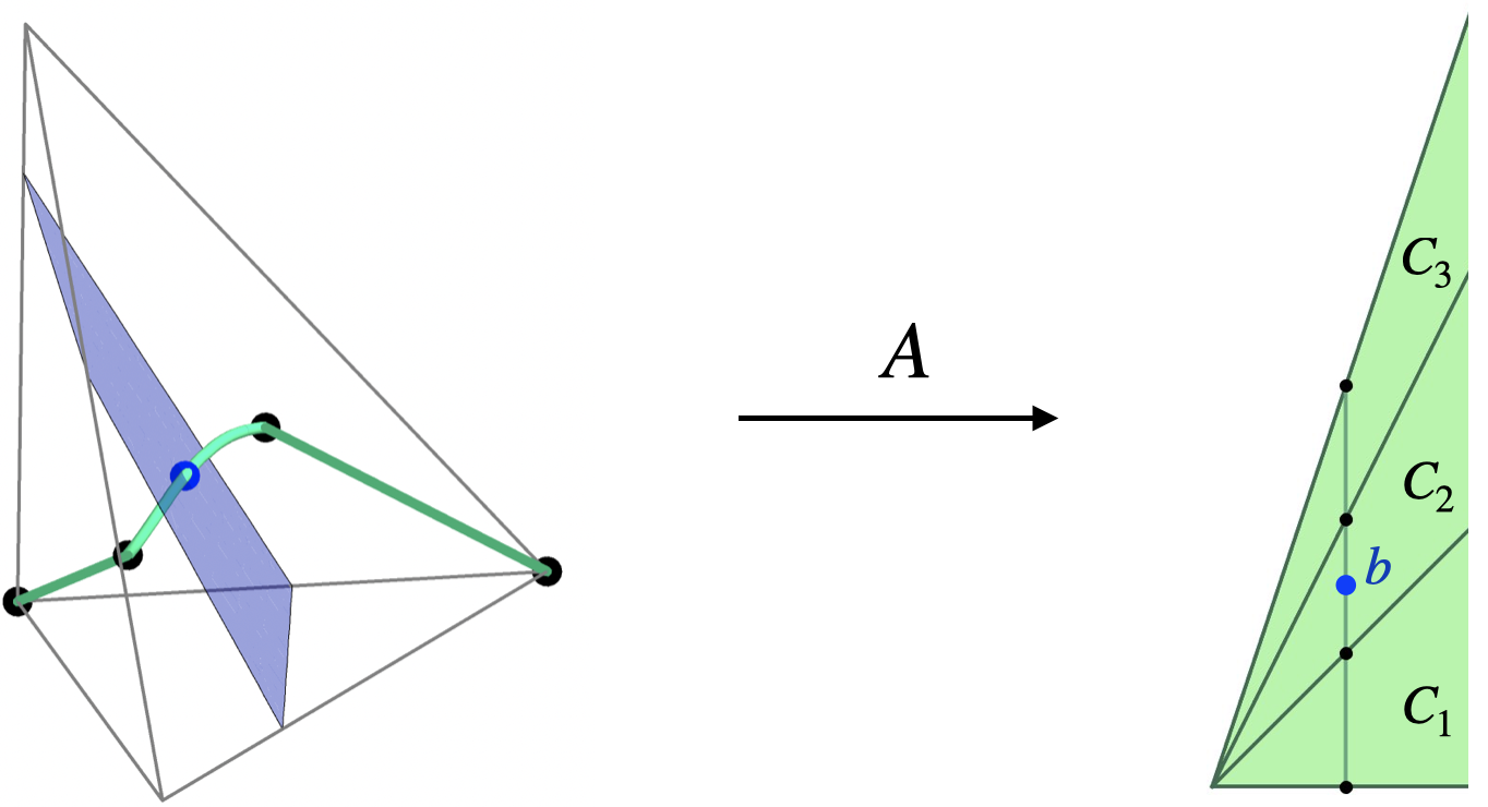
Figure 4: The Santaló patchwork (left) and chamber complex (right) from Example 3.6.

Example 3.7.

The Santaló patchwork for the matrix $A$ in our running example (Example 1.2) consists of 11 patches, one for each cell in the chamber complex shown in Example 1.1. These 11 patches are separated by the black curves on the surfaces in Figure 2.

The following statement is a tautology. It emphasizes the role of ${\rm SP}(A)$ in solving (5).

Proposition 3.8.

The Santaló point of $P_{b}$ is given by $x^{*}(b)=\phi(b)={\rm SP}(A)\cap P_{b}$.

Example 3.9.

For $A$ as in Example 3.5, the polytope $P_{b}$ for $b=(1,2)$ is the blue line segment in Figure 3 (left). Its blue intersection point with ${\rm SP}(A)$ is the center of that line segment, which is its Santaló point $x^{*}(b)$. For $A$ as in Example 3.6, the polytope $P_{b}$ for $b=(1,3/2)$ is the blue quadrilateral in Figure 4. Again, ${\rm SP}(A)\cap P_{b}$ is the Santaló point.

4 Patch varieties

Section 3 describes the set of all solutions to the optimization problem (5) as a semi-algebraic set called the Santaló patchwork. For algebraic computations, it is often convenient to work with algebraic sets instead. This section studies algebraic varieties containing the Santaló patches $S_{C}$ defined in (18). A natural thing to do is take the Zariski closure. We define

$$X_{C}\,=\,\overline{S_{C}}\,\subset\,\mathbb{C}^{n}.$$

We call $X_{C}$ the patch variety of the cell $C$. A simple way to find equations vanishing on $X_{C}$ is by dropping the inequalities in (18). Let ${\cal X}_{C}\subset\mathbb{C}^{n}$ be the Zariski closure of the set

$${\cal X}_{C}^{\circ}\,=\,\left\{x\in\mathbb{C}^{n}\,:\,\alpha_{C}(x)\prod_{i\in{\cal F}_{C}}x_{i}\neq 0\quad\text{and}\quad B_{C}^{T}\cdot\left(\frac{\partial_{x_{i}}\alpha_{C}}{\alpha_{C}}-\frac{1}{x_{i}}\right)_{i\in{\cal F}_{C}}\,=\,0\right\}.$$

Theorem 4.1.

The patch variety $X_{C}$ is a $d$-dimensional irreducible component of ${\cal X}_{C}$.

Proof 4.2.

We switch to $(b,y)$-coordinates using the transformation from (11). We view

$$B_{C}^{T}\cdot\left(\frac{\partial_{x_{i}}\alpha_{C}}{\alpha_{C}}-\frac{1}{x_{i}}\right)_{i\in{\cal F}_{C}}\,=\,0$$ (19)

as equations in $y$, parametrized by $b$. For $b_{0}\in C\cap{\rm pos}(A)$, by strict convexity of $V_{C}(x)$, the Santaló point $x^{*}(b_{0})\sim(b_{0},y^{*}(b_{0}))$ corresponds to an isolated solution. By [33, Theorem A.14.1], it follows that $x^{*}(b_{0})$ lies on a $d$-dimensional irreducible component ${\cal Z}^{\circ}$ of ${\cal X}_{C}^{\circ}$, and hence on an irreducible component ${\cal Z}=\overline{{\cal Z}^{\circ}}$ of ${\cal X}_{C}$. This is true for every $b_{0}\in C\cap{\rm pos}(A)$, so that $S_{C}$ is contained in ${\cal Z}$. Hence, $X_{C}\subset{\cal Z}$ and it has dimension at most $d$. By Corollary 3.4, $S_{C}$ is $d$-dimensional, so $X_{C}$ has dimension at least $d$. We conclude that $X_{C}={\cal Z}\subset{\cal X}_{C}$.

Notice that, by construction, the Santaló patch $S_{C}$ is stable under simultaneous scaling of the coordinates: $x^{*}(t\cdot b)=t\cdot x^{*}(b)$ for any $t\in\mathbb{R}_{>0}$. It follows that the ideal of $X_{C}$ can be generated by homogeneous equations. Furthermore, since the equations defining ${\cal X}^{\circ}_{C}$ are homogeneous (of degree $-1$), $I({\cal X}_{C})$ is a homogeneous ideal as well.

If $A\in\mathbb{Q}^{d\times n}_{\geq 0}$ has rational entries, the vanishing ideal $I({\cal X}_{C})$ of ${\cal X}_{C}$ can be computed using computer algebra software such as Macaulay2 [15] or Oscar.jl [30] as follows. Consider the ideal of the ring $\mathbb{Q}[(x_{i})_{i\in{\cal F}_{C}},(\sigma_{i})_{i\in{\cal F}_{C}},z]$ generated by the $n-d+n_{C}+1$ equations

$$B_{C}^{T}\cdot\left(z\,\partial_{x_{i}}\alpha_{C}-\sigma_{i}\right)_{i\in{\cal F}_{C}},\quad x_{i}\sigma_{i}-1,i\in{\cal F}_{C},\quad\text{and}\quad\,\alpha_{C}(x)\,z-1.$$

From this ideal, eliminate the variables $\sigma_{i},i\in{\cal F}_{C}$ and $z$. The result is $I({\cal X}_{C})$.

Example 4.3.

We perform the computation explained above for our running Example 1.2, for the 3-dimensional cell $C\in{\cal C}_{A}$ with five facets containing $b=(1,4/5,4/5)$. The adjoint is

$$\alpha_{C}(x)\,=\,3x_{1}x_{2}x_{3}+2x_{1}x_{3}x_{5}+2x_{1}x_{4}x_{5}+2x_{2}x_{3}x_{4}+2x_{2}x_{4}x_{5},$$

i.e., the numerator of (4). The elimination takes place in a polynomial ring with $11$ variables. The ideal $I({\cal X}_{C})$ is prime, homogeneous, and of degree $14$. It is generated by five quintics. Here is how to compute $\alpha_{C}$ and $I({\cal X}_{C})$ using our Julia package Santalo.jl, available at the online repository https://mathrepo.mis.mpg.de/Santalo:

⬇

using Santalo # load the package

A = [1 1 1 1 1; 2 1 0 1 0; 1 2 0 0 1]; b = 1//5*[5; 4; 4];

R, alpha = adjoint_x(A,b)

T, J = ideal_XC(A,b)

The outputs in line 3 are the adjoint alpha $=\alpha_{C}$ and a polynomial ring R containing it. In line 4, we compute the ideal J $=I({\cal X}_{C})$ and a polynomial ring T containing it.

Next, we ask whether ${\cal X}_{C}$ may fail to be equidimensional. I.e., can it have components of dimension $>d$? We do not know the answer, but we expect that for general matrices we even have $X_{C}={\cal X}_{C}$ (see Conjecture 4.10). We show that the answer is no if we perturb the objective function $V_{C}(x)$ slightly. More precisely, we consider the new objective function

$$V_{C,u}(x)\,=\,\frac{\alpha_{C}(x)^{u_{0}}}{\prod_{i\in{\cal F}_{C}}x_{i}^{u_{i}}}.$$ (20)

Here $u_{0},u_{i},i\in{\cal F}_{C}$ are new parameters. Setting $u={\bf 1}=(1,\ldots,1)$ recovers our original objective function $V_{C}$. We will see in Section 4 that these new parameters have a natural statistical interpretation. The critical point equations of $\log V_{C,u}$ define the incidence

$$\mathscr{X}_{C}^{\circ}\,=\,\left\{(x,u)\in\mathbb{C}^{n}\times\mathbb{C}^{n_{C}+1}\,:\,\alpha_{C}(x)\prod_{i\in{\cal F}_{C}}x_{i}\neq 0\quad\text{and}\quad B_{C}^{T}\cdot\left(\frac{u_{0}\partial_{x_{i}}\alpha_{C}}{\alpha_{C}}-\frac{u_{i}}{x_{i}}\right)_{i\in{\cal F}_{C}}=\,0\right\}.$$

We write $\pi_{u}:\mathscr{X}_{C}^{\circ}\rightarrow\mathbb{C}^{n_{C}+1}$ for the projection $(x,u)\mapsto u$, and denote its fiber $\pi_{u}^{-1}(u)$ by $\mathscr{X}^{\circ}_{C,u}$. The variety ${\cal X}^{\circ}_{C}$ is $\mathscr{X}_{C,{\bf 1}}^{\circ}$. The Zariski closure of $\mathscr{X}^{\circ}_{C}$ is $\mathscr{X}_{C}\subset\mathbb{C}^{n}\times\mathbb{C}^{n_{C}+1}$. Fibers of $\pi_{u}:\mathscr{X}_{C}\rightarrow\mathbb{C}^{n_{C}+1}$ are denoted by $\mathscr{X}_{C,u}$. We have $\overline{\mathscr{X}_{C,u}^{\circ}}\subset\mathscr{X}_{C,u}$, and in particular ${\cal X}_{C}\subset\mathscr{X}_{C,{\bf 1}}$.

Proposition 4.4.

The varieties $\mathscr{X}_{C}^{\circ},\mathscr{X}_{C}$ are irreducible of dimension $n_{C}+1+d$. There is a dense open subset $U\subset\mathbb{C}^{n_{C}+1}$ such that, for $u\in U$, $\mathscr{X}_{C,u}$ is pure dimensional of dimension $d$.

Proof 4.5.

We consider the other projection $\pi_{x}:\mathscr{X}_{C}^{\circ}\rightarrow\mathbb{C}^{n}$ which sends $(x,u)$ to $x$. A fiber $\pi_{x}^{-1}(x)$ is defined by linear equations in $u_{0},u_{i},i\in{\cal F}_{C}$. These equations are linearly independent, because $B_{C}$ has rank $n-d$. This last claim follows from the fact that the rows of $B$ giving rise to $B_{C}$ are indexed by $\mathcal{F}_{C}$, which means that they contain the rays of the normal fan to a full-dimensional polytope $Q_{b}$ for $b\in\mathrm{int}(C)$. Hence, all fibers of $\pi_{x}$ are linear, and hence irreducible, of dimension $n_{c}+1-n+d$. By [32, Chapter 1, §6, Theorem 8], $\mathscr{X}^{\circ}_{C}$ is irreducible of dimension $n_{C}+1+d$. The same holds for $\mathscr{X}_{C}$. Since the map $\pi_{u}:\mathscr{X}_{C}\rightarrow\mathbb{C}^{n_{C}+1}$ is dominant, the proposition now follows from [32, Chapter 1, §6, Theorem 7].

The following statement summarizes the role of these varieties in the study of the Santaló point of $P_{b}$: they provide useful semi-algebraic descriptions.

Theorem 4.6.

Let $b\in C\cap{\rm pos}(A)$ for some cell $C\in{\cal C}_{A}$ and let $P_{b}^{\circ}={\rm relint}(P_{b})$. The Santaló point $x^{*}(b)$ is given by

$$x^{*}(b)\,=\,{\rm SP}(A)\cap P_{b}^{\circ}\,=\,S_{C}\cap P_{b}^{\circ}\,=\,X_{C}\cap P_{b}^{\circ}\,=\,{\cal X}_{C}^{\circ}\cap P_{b}^{\circ}\,=\,{\cal X}_{C}\cap P_{b}^{\circ}\,=\,\mathscr{X}_{C,{\bf 1}}^{\circ}\cap P_{b}^{\circ}\,=\,\mathscr{X}_{C,{\bf 1}}\cap P_{b}^{\circ}.$$

Proof 4.7.

The first two equalities are essentially Proposition 3.8. The equality $x^{*}(b)={\cal X}_{C}^{\circ}\cap P_{b}^{\circ}$ follows from strict convexity of the dual volume function on $P_{b}$: there is only one critical point of $\log V_{C}$ on $P_{b}^{\circ}$. Since $({\cal X}_{C}\setminus{\cal X}_{C}^{\circ})\cap\mathbb{R}^{n}_{>0}=\emptyset$, replacing ${\cal X}_{C}^{\circ}$ with ${\cal X}_{C}$ does not change the intersection with $P_{b}^{\circ}$. The equality $x^{*}(b)=X_{C}\cap P_{b}^{\circ}$ now follows from $x^{*}(b)\in X_{C}\subset{\cal X}_{C}$. The last two equalities follow from $\mathscr{X}_{C,{\bf 1}}^{\circ}={\cal X}_{C}^{\circ}$ and $(\mathscr{X}_{C,{\bf 1}}\setminus\mathscr{X}_{C,{\bf 1}}^{\circ})\cap\mathbb{R}^{n}_{>0}=\emptyset$.

Next, we state a naive degree bound for the varieties defined in this section.

Proposition 4.8.

For $\bullet=X_{C},{\cal X}_{C}$ or $\mathscr{X}_{C,u}$, for generic $u$, we have the inequality

$$\deg(\bullet)\leq(2n_{C}-n+d-1)^{n-d}.$$

Proof 4.9.

For ${\cal X}_{C}$, this follows from clearing denominators in (19) and applying Bézout’s bound [17, Chapter I, Theorem 7.7]. For $X_{C}$, we use Theorem 4.1. Finally, for $\mathscr{X}_{C,u}$, note that for generic $u\in\mathbb{C}^{n_{C}+1}$ we have $\mathscr{X}_{C,u}=\overline{\mathscr{X}_{C,u}^{\circ}}$. Adding the parameters $u$ to the equations (19) does not change the Bézout number.

The bound from Proposition 4.8 is pessimistic. E.g., for Example 4.3 it reads $14\leq 49$. In particular, the varieties $X_{C}={\cal X}_{C}$ and $\mathscr{X}_{C,u}$ have the same degree in that example. In the next section, we use insights from algebraic statistics to prove a lower bound on $\deg\mathscr{X}_{C,u}$ for generic $u$ (Corollary 5.9). That bound is relevant for our homotopy method for computing Santaló points in Section 6. Also, in experiments, we find that it approximates the actual degree more closely (Example 5.14). As motivated by the next conjecture, which is suggested by the examples we computed, we here mean both the degree of $X_{C}$ and $\mathscr{X}_{C,u}$.

Conjecture 4.10.

For generic matrices $A\in\mathbb{R}^{d\times n}_{\geq 0}$ and for each cell $C\in{\cal C}_{A}$, there exists a dense open subset $U\subset\mathbb{C}^{n_{C}+1}$ such that the variety $\mathscr{X}_{C,u}$ is irreducible of dimension $d$ for $u\in U$. Moreover, ${\bf 1}\in U$ and we have $\mathscr{X}_{C,{\bf 1}}={\cal X}_{C}=X_{C}$.

5 Wachspress models

In algebraic statistics [11, 35], a statistical model for a discrete random variable with $N+1$ states is the intersection of a complex algebraic variety $M_{\mathbb{C}}$ with the probability simplex

$$\Delta_{N}\,=\,\{(p_{0},\ldots,p_{N})\in\mathbb{R}^{N+1}_{>0}\,:\,p_{0}+\cdots+p_{N}=1\}.$$

We denote this model by $M=M_{\mathbb{C}}\cap\Delta_{N}$, and require that this intersection is non-empty. For our purposes, it suffices to consider parametric models, i.e., models that come with a rational parametrization. This is true for many commonly used models, including exponential families and (conditional) independence models. Let $p_{i}(y)=p_{i}(y_{1},\ldots,y_{m}),i=0,\ldots,N$ be rational functions of $m<N$ variables such that $\sum_{i=0}^{N}p_{i}=1$. The variety $M_{\mathbb{C}}$ is the closure of the image of the rational map $\mathbb{C}^{m}\dashrightarrow\mathbb{C}^{N+1}$ given by $y\mapsto(p_{0}(y),\ldots,p_{N}(y))$. Maximum likelihood estimation for the model $M$ means finding the probability distribution $p\in M$ which makes an experimental observation $u\in\mathbb{N}^{N+1}$ most likely. More precisely, suppose that state $i$ was observed $u_{i}$ times in an experiment. One maximizes the log-likelihood function

$$L_{u}\,=\,\log p_{0}^{u_{0}}p_{1}^{u_{1}}\cdots p_{N}^{u_{N}}$$

subject to the constraint $p\in M$. To study this problem algebraically, one often relaxes it to finding all complex critical points of $L_{u}$ on an open subset of $M_{\mathbb{C}}$. In our parametric setting, we solve the system of rational function equations

$$\partial_{y_{i}}L_{u}(y)\,=\,\sum_{j=0}^{N}u_{j}\,\frac{\partial_{y_{i}}p_{j}(y)}{p_{j}(y)}=\,0,\quad i=1,\ldots m\quad\text{for}\quad y\in\mathbb{C}^{m}\setminus D.$$ (21)

Here $D\subset\mathbb{C}^{m}$ is the union of the supports of the divisors ${\rm div}(p_{j}),j=0,\ldots,N$. That is, it is the union of all hypersurfaces in $\mathbb{C}^{m}$ along which one of the $p_{j}$ has a zero or a pole. We refer to these equations as the likelihood equations for the model $M$. The number of complex solutions $y\in\mathbb{C}^{m}\setminus D$ for generic, complex data $u\in\mathbb{C}^{N+1}$ is an invariant called the maximum likelihood degree (ML degree) of $M_{\mathbb{C}}$ [8], which we denote by ${\rm MLdeg}(M_{\mathbb{C}})$. This assumes that the parametrization map $\mathbb{C}^{m}\setminus D\rightarrow M_{\mathbb{C}}$ given by $y\mapsto(p_{0}(y),\ldots,p_{N}(y))$ is birational.

The models that are relevant to our story are called Wachspress models. These are associated to a simple polytope $Q\subset\mathbb{R}^{m}$, and the number of states equals the number of vertices $|{\cal V}(Q)|$. We use the notation (8) for the face description of $Q$. The parametrizing functions of our model are naturally obtained from the formula (10) for the adjoint:

$$p_{v}(y)\,=\,\frac{|\det W_{I(v)}|\cdot\prod_{i\notin I(v)}(c_{i}+\langle w_{i},y\rangle)}{\alpha_{Q}(y)},\quad v\in{\cal V}(Q).$$ (22)

This gives a rational map $\mathbb{C}^{m}\dashrightarrow\mathbb{P}^{|{\cal V}(Q)|-1}$, whose image closure $M_{\mathbb{C}}(Q)$ is the Wachspress variety of $Q$. Note that the coordinates $p_{v}$ for $v\in{\cal V}(Q)$ sum to 1 by construction. These varieties appear in the context of geometric modelling [14], and Wachspress surfaces were studied in [21]. To the best of our knowledge, the interpretation as a statistical model first appeared in [24]. Bayesian integrals for these models were studied in [6]. The divisor $D$ from (21) for the Wachspress model $M_{\mathbb{C}}(Q)$ is the union of the adjoint hypersurface $\alpha_{Q}(y)=0$ and the facet hyperplanes $c_{i}+\langle w_{i},y\rangle=0$. We denote this hypersurface by $D(Q)$.

Lemma 5.1.

Let $Q\subset\mathbb{R}^{m}$ be a simple polytope with Wachspress model $M_{\mathbb{C}}(Q)$. Let ${\cal H}\subset\mathbb{P}^{N}$ be the divisor $(\sum_{i=0}^{N}p_{i})\prod_{i=0}^{N}p_{i}=0$ for $N=|{\cal V}(Q)|-1$. The map $\psi\!:\!\mathbb{C}^{m}\setminus D(Q)\rightarrow M_{\mathbb{C}}(Q)\setminus{\cal H}$ given by $y\mapsto(p_{v}(y))_{v\in{\cal V}(Q)}$, with $p_{v}$ from (22), is an isomorphism.

Proof 5.2.

First note that the morphism $\psi$ is well-defined. The functions $p_{v}$ are regular on $\mathbb{C}^{m}\setminus D(Q)$, and the image of $\mathbb{C}^{m}\setminus D(Q)$ is contained in the complement of ${\cal H}$.

It remains to show that $\psi$ is invertible. Consider an automorphism $\varphi$ of $\mathbb{P}^{N}$ defined by $p_{v}\mapsto\frac{p_{v}}{|\det W_{I(v)}|}$. The map $\varphi\circ\psi$ is a restriction of the Wachspress map defined in [23, Equation (5)], which is invertible by [23, Theorem 4]. It follows that $\psi$ is invertible too.

Corollary 5.3.

The maximum likelihood degree ${\rm MLdeg}(M_{\mathbb{C}}(Q))$ of the Wachspress model of $Q$ equals the absolute value of the Euler characteristic $\chi(\mathbb{C}^{m}\setminus D(Q))=\chi(M_{\mathbb{C}}(Q)\setminus{\cal H})$.

Proof 5.4.

By Lemma 5.1, $M_{\mathbb{C}}(Q)\setminus{\cal H}$ is smooth, so [20, Theorem 1.7] implies the statement.

Solving the likelihood equations of $M_{\mathbb{C}}(Q)$ with data $u$ is equivalent to computing the intersection of the fiber $\mathscr{X}_{C,u^{\prime}}^{\circ}$, defined in Section 3, with a linear space. The parameters $u^{\prime}\in\mathbb{C}^{n_{C}+1}$ are obtained from $u$ via a linear map. This is the content of our next theorem.

Theorem 5.5.

Let $Q_{b_{0}}=B^{T}\cdot P_{b_{0}}$ for $b_{0}\in C\cap{\rm pos}(A)$, where $C\in{\cal C}_{A}$ is a cell in the chamber complex of $A$. The complex critical points of the log-likelihood function $L_{u}(y)$ for the Wachspress model $M_{\mathbb{C}}(Q_{b_{0}})$ with data $u=(u_{v})_{v\in{\cal V}(Q_{b_{0}})}$ are in one-to-one correspondence with the complex critical points of $V_{C,u^{\prime}}(x)$ from (20) on $\{Ax={b_{0}}\}$, where $u^{\prime}$ has entries

$$u_{0}^{\prime}\,=\,-\sum_{v\in{\cal V}(Q_{b})}u_{v},\quad u_{i}^{\prime}\,=\,-\sum_{v:i\notin I(v)}u_{v},\,i\in{\cal F}_{C}.$$ (23)

More precisely, the critical points $y_{\rm crit}\in\mathbb{C}^{n-d}\setminus D(Q_{b_{0}})$ of $L_{u}(y)$ are $B^{T}\cdot x_{\rm crit}$, where $x_{\rm crit}$ ranges over the points in the intersection $\mathscr{X}_{C,u^{\prime}}^{\circ}\cap\{A\,x={b_{0}}\}$,

Proof 5.6.

The likelihood function for the data $u=(u_{v})_{v\in{\cal V}(Q_{b_{0}})}$ is

$${\rm exp}\,L_{u}(y)=\prod_{v\in{\cal V}(Q_{b_{0}})}\left(\frac{|\det W_{I(v)}|\cdot\prod_{i\in{\cal F}_{C}\setminus I(v)}(c_{i}(b_{0})+\langle w_{i},y\rangle)}{\alpha_{Q_{b_{0}}}(y)}\right)^{u_{v}}=V_{C,u^{\prime}}\left(\begin{pmatrix}A\\ B^{T}\end{pmatrix}^{-1}\begin{pmatrix}b_{0}\\ y\end{pmatrix}\right).$$

This uses the change of coordinates (11): $x_{i}=c_{i}(b_{0})+\langle w_{i},y\rangle$. Applying the chain rule gives

$$\partial_{y_{j}}\log V_{C,u^{\prime}}\,=\,\sum_{i\in{\cal F}_{C}}\partial_{x_{i}}\log V_{C,u^{\prime}}\cdot\frac{{\rm d}x_{i}}{{\rm d}y_{j}}.$$

It follows that the likelihood equations for the Wachspress model $M_{\mathbb{C}}(Q_{b_{0}})$ are equivalent to

$$W_{C}^{T}\cdot\left(\frac{u_{0}^{\prime}\partial_{x_{i}}\alpha_{C}}{\alpha_{C}}-\frac{u_{i}^{\prime}}{x_{i}}\right)_{i\in{\cal F}_{C}}=\,0\quad\text{and}\quad Ax\,=\,b_{0}.$$

Here $Ax=b_{0}$ is $b=b_{0}$ in $x$-coordinates, and $W_{C}$ is the submatrix of the matrix $W$ of facet normals whose rows are indexed by ${\cal F}_{C}$. The column span of $W_{C}$ equals that of $B_{C}$ by construction, so these are precisely the equations for $\mathscr{X}_{C,u^{\prime}}^{\circ}\cap\{Ax=b_{0}\}$.

Our next statement uses the following definition. An isolated solution $x$ to the $n$ equations

$$B_{C}^{T}\cdot\left(\frac{\tilde{u}_{0}\partial_{x_{i}}\alpha_{C}}{\alpha_{C}}-\frac{\tilde{u}_{i}}{x_{i}}\right)_{i\in{\cal F}_{C}}=\,0\quad\text{and}\quad Ax=b_{0}$$ (24)

for fixed $\tilde{u}\in\mathbb{C}^{n_{C}+1}$ is regular if the rank of the Jacobian matrix at $x$ is $n$.

Proposition 5.7.

Let $b_{0}\in C\cap{\rm pos}(A)$ for some cell $C\in{\cal C}_{A}$. There is a dense open subset $U\subset\mathbb{C}^{n_{C}+1}$ such that, for $\tilde{u}\in U$, the set $I(\tilde{u},b_{0}):=\mathscr{X}_{C,\tilde{u}}^{\circ}\cap\{Ax=b_{0}\}$ consists of ${\rm MLdeg}(M_{\mathbb{C}}(Q_{b_{0}}))$ regular points. Moreover, the number of regular isolated points in $I(\tilde{u},b_{0})$ for any $\tilde{u}$ is at most ${\rm MLdeg}(M_{\mathbb{C}}(Q_{b_{0}}))$.

Proof 5.8.

The data points $u=(u_{v})_{v\in{\cal V}(Q_{b_{0}})}$ for the Wachspress model $M_{\mathbb{C}}(Q_{b_{0}})$ parametrize a linear subspace $H$ of $\mathbb{C}^{n_{C}+1}$ via (23). By Theorem 5.5 and the definition of the ML degree, the number of points in $I(u^{\prime},b_{0})$ is ${\rm MLdeg}(M_{\mathbb{C}}(Q_{b_{0}}))$ for generic $u^{\prime}\in H$. By Corollary 5.3, this number equals the signed Euler characteristic of $\mathbb{C}^{m}\setminus D(Q_{b_{0}})$. By [19, Theorem 1], that Euler characteristic is the number of regular complex critical points of

$$V_{C,\tilde{u}}\left(\begin{pmatrix}A\\ B^{T}\end{pmatrix}^{-1}\begin{pmatrix}b_{0}\\ y\end{pmatrix}\right)\,=\,\frac{\alpha_{Q_{b_{0}}}(y)^{\tilde{u}_{0}}}{\prod_{i\in{\cal F}_{C}}(c_{i}(b_{0})+\langle w_{i},y\rangle)^{\tilde{u}_{i}}}.$$

for generic $\tilde{u}\in\mathbb{C}^{n_{C}+1}$. The final statement about the upper bound follows from the fact that the generic number of regular isolated solutions to the system of equations (24) equals the maximal number of regular isolated solutions, see for instance [33, Theorem 7.1.1].

Corollary 5.9.

For any cell $C\in{\cal C}_{A}$ and generic $\tilde{u}\in\mathbb{C}^{n_{C}+1}$ the degree of the variety $\mathscr{X}_{C,\tilde{u}}\subset\mathbb{C}^{n}$ is at least ${\rm MLdeg}(M_{\mathbb{C}}(Q_{b_{0}}))$, where $b_{0}$ is a generic point in ${\rm int}(C)$.

Proof 5.10.

By Proposition 4.4, $\mathscr{X}_{C,\tilde{u}}$ is pure dimensional of dimension $d$ for generic $u$. Its degree is the maximal number of regular intersection points with a linear space of codimension $d$. This is at least the cardinality of $I(\tilde{u},b_{0})$. The statement is a consequence of Proposition 5.7.

Though the Santaló point of $Q_{b_{0}}$ is one of the regular intersection points in $I({\bf 1},b_{0})=\mathscr{X}^{\circ}_{C,\bf{1}}\cap\{Ax=b_{0}\}$ (Theorem 4.6), the usefulness of the results in this section for our original problem may seem somewhat mysterious. It will become clear in Section 6 that Proposition 5.7 is crucial for our homotopy continuation based algorithm for computing Santaló points.

Remark 5.11.

Dual volume minimization is not the only convex optimization problem on $P_{b}$ that has the interpretation of a maximum likelihood estimation problem. Other commonly used objective functions lead to maximum likelihood estimation for different models. We briefly discuss the cases $V(x)=-\sum_{i=1}^{n}\log x_{i}$ (log-barrier) and $V(x)=\sum_{i=1}^{n}x_{i}\log x_{i}-x_{i}$ (entropic regularization) mentioned in the Introduction. In each case, there are $N+1=n$ states. For ease of exposition, we make some additional assumptions on the matrix $A$.

First, for $V(x)=-\sum_{i=1}^{n}\log x_{i}$, assume that the entries of each column of $A$ sum to the same number $c$. The statistical model $M$ in this context is the linear model obtained by intersecting the row span $M_{\mathbb{C}}$ of $A$ with $\Delta_{n-1}$. It is parametrized by $p_{i}(y)=(y^{T}a_{i})/(y^{T}A{\bf 1})$, where $a_{i}$ is the $i$-th column of $A$ and ${\bf 1}\in\mathbb{R}^{n}$ is the all-ones vector. One checks that the maximum likelihood estimate for the data $u=(1,\ldots,1)$ is the unique positive minimizer of the log-barrier function $V(x)$ on the affine-linear space $\{Ax=b\}$, where $b=c^{-1}\,A\,{\bf 1}$.

For $V(x)=\sum_{i=1}^{n}x_{i}\log x_{i}-x_{i}$, the model comes from a toric variety. We assume that the first row of $A$ is the all-ones vector ${\bf 1}$ and write $a_{i}\in\mathbb{R}^{d}_{\geq 0}$ for the $i$-th column. These columns define a monomial map, whose image is $M_{\mathbb{C}}$. Concretely, let $f(y)=y^{a_{1}}+y^{a_{2}}+\cdots+y^{a_{n}}$ and consider the rational parametrization functions $p_{i}(y)=y^{a_{i}}/f(x)$, parametrizing $M_{\mathbb{C}}$. For any data vector $u=(u_{1},\ldots,u_{n})\in\mathbb{N}^{n}$, let $\bar{u}=(\sum_{i=1}^{n}u_{i})^{-1}\cdot u$ be the empirical distribution. As a consequence of Birch’s theorem [11, Proposition 2.1.5], the maximum likelihood estimate for the model $M$ is the unique positive minimizer of the entropy $V(x)$ on $\{Ax=A\bar{u}\}$.

There is no explicit formula for the maximum likelihood degree of the Wachspress model $M_{\mathbb{C}}(Q)$. We end the section with conjectures for polygons in the plane. We represent a generic $n$-gon by a fiber $P_{b}$ of $A:\mathbb{R}^{n}_{\geq 0}\rightarrow{\rm cone}(A)$, where $A\in\mathbb{R}^{(n-2)\times n}_{\geq 0}$ is generic among those matrices for which there is a cell in ${\cal C}_{A}$ whose fibers are $n$-gons. Concretely, let

$$C_{\max}\,=\,{\rm cone}(A_{[n]\setminus\{1\}})\cap{\rm cone}(A_{[n]\setminus\{2\}})\cap\cdots\cap{\rm cone}(A_{[n]\setminus\{n\}})\,\neq\,\emptyset\quad\text{and}\quad\dim(C_{\max})=n-2.$$

This uses the notation introduced before Definition 2.3. In general, $C_{\max}$ is a union of cells in ${\cal C}_{A}$. We pick $b\in{\rm int}(C)$ for any cell $C\subset C_{\max}$.

Conjecture 5.12.

Let $Q=B^{T}\cdot P_{b}$ be a generic $n$-gon. The maximum likelihood degree of the corresponding Wachspress model is ${\rm MLdeg}(M_{\mathbb{C}}(Q))=(n-1)(n-2)+(n-3)(n-5)-1$.

Proof 5.13 (Sketch of proof).

By Corollary 5.3, we have ${\rm MLdeg}(M_{\mathbb{C}}(Q))=\chi(\mathbb{C}^{2}\setminus D(Q))$, where $D_{Q}$ is the curve $\{\alpha_{Q}(y)\prod_{i=1}^{n}l_{i}(y)=0\}$. Here we write $l_{i}(y)=c_{i}+\langle w_{i},y\rangle$ for the equations of the lines defining the edges of $Q$. The excision property of the Euler characteristic gives

$$\chi(\mathbb{C}^{2}\setminus D(Q))\,=\,\chi\big{(}\mathbb{C}^{2}\setminus\big{\{}\prod_{i=1}^{n}l_{i}(y)=0\big{\}}\big{)}\,-\,\chi\big{(}\{\alpha_{Q}(y)=0\}\setminus\big{\{}\prod_{i=1}^{n}l_{i}(y)=0\big{\}}\big{)}.$$

Since the line arrangement of $l_{1},\ldots,l_{n}$ is generic, the first term is $\binom{n-1}{2}$ [18, Equation (8)]. On the second term, we use excision once more:

$$\chi\big{(}\{\alpha_{Q}(y)=0\}\setminus\big{\{}\prod_{i=1}^{n}l_{i}(y)=0\big{\}}\big{)}\,=\,\chi(\{\alpha_{Q}(y)=0\})-\chi\big{(}\{\alpha_{Q}=0\}\cap\big{\{}\prod_{i=1}^{n}l_{i}(y)=0\big{\}}\big{)}.$$

Here the second term is $-\binom{n-1}{2}-1$, the number of residual points of $Q$ [22, Section 2.1]. What’s missing is the Euler characteristic of the affine curve $\chi(\{\alpha_{Q}(y)=0\}$. We conjecture that, for generic $Q$, this curve is generic in the sense of [19, Theorem 3], with Newton polytope equal to that of $(1+y_{1}+y_{2})^{n-3}$. That would imply that its Euler characteristic equals $-(n-3)^{2}+2(n-3)$. Summing all this up gives the formula in the conjecture.

In the spirit of Corollary 5.9, we can compare the number $(n-1)(n-2)+(n-3)(n-5)-1$ to the degree of the variety $\mathscr{X}_{C,u}$, and hence that of ${\cal X}_{C}$ and $X_{C}$ (Conjecture 4.10).

Example 5.14.

For $n=3,4,\ldots,11$ we generate a totally positive matrix $A\in(\mathbb{R})^{(n-2)\times n}_{\geq 0}$ (meaning that all $(n-2)$-minors are positive) and we pick a cell $C\subset C_{\max}$. Using the numerical homotopy continuation techniques discussed in the next section, we compute that

$n$	3	4	5	6	7	8	9	10	11
$(n-1)(n-2)+(n-3)(n-5)-1$	1	4	11	22	37	56	79	106	137
$\deg(\mathscr{X}_{C,u})=\deg({\cal X}_{C})=\deg(X_{C})$	1	4	14	27	44	65	90	119	152

For instance, for $n=5$, a generic linear space $\{\tilde{A}x=\tilde{b}\}$ of dimension 2 intersects $\mathscr{X}_{C,u}$ in 14 points. By Proposition 5.7, the special linear space $\{Ax=b\}$ leads to only 11 points. Hence, the lower bound in 5.9 may be strict. The table leads us to conjecture that for $n\geq 5$,

$$\deg(X_{C})\,=\,(n-1)(n-2)+(n-3)(n-5)-1+2(n-3)-1.$$

Code for computing these degrees is found at https://mathrepo.mis.mpg.de/Santalo.

6 Computing Santaló points

We discuss how to compute Santaló points numerically. We consider two different situations. First, the input is a polytope $Q\subset\mathbb{R}^{m}$, and the output is its Santaló point $y^{*}$ from (1). Our continuation algorithm exploits the likelihood geometry from Section 5. The second scenario computes the Santaló point $x^{*}(b_{1})$ from $x^{*}(b_{0})$, assuming $b_{1}$ lies in the same cell $C\in{\cal C}_{A}$ as $b_{0}$. The strategy here is to track a real path on the Santaló patch $S_{C}$. These algorithms are implemented in Julia (v1.9.1) using Oscar.jl (v0.14.0) [30] and HomotopyContinuation.jl (v2.9.3) [7]. All code is available at https://mathrepo.mis.mpg.de/Santalo.

The computational paradigm behind our algorithms is that of homotopy continuation. We briefly recall the main idea and refer to the standard textbook [33] for more details. Let $F:(\mathbb{C}^{n}\setminus D)\times\mathbb{C}^{m}\rightarrow\mathbb{C}^{n}$ be a map whose coordinates are rational functions in $x=(x_{1},\ldots,x_{n})$, depending polynomially on $m$ parameters $q=(q_{1},\ldots,q_{m})$. We assume that the denominators of these functions do not depend on $q$, and their vanishing locus is contained in the hypersurface $D\subset\mathbb{C}^{n}$, so that $F$ is a regular map. We consider the incidence variety

$$Y\,=\,F^{-1}(0)\,=\,\{(x,q)\in(\mathbb{C}^{n}\setminus D)\times\mathbb{C}^{m}\,:\,F(x,q)=0\}.$$

A fiber of the natural projection $\pi_{q}:Y\rightarrow\mathbb{C}^{m}$ is denoted by $Y_{q_{0}}=\pi_{q}^{-1}(q_{0})$. It consists of all solutions to the $n$ equations in $n$ variables $F(x,q_{0})=0$. A solution $(x_{0},q_{0})$ in $Y_{q_{0}}$ is called isolated and regular if the Jacobian of $F$ (with respect to $x$) evaluated at $(x_{0},q_{0})$ is an invertible $n\times n$-matrix. Typically, one has computed all isolated regular solutions in $Y_{q_{0}}$ and is interested in computing those in $Y_{q_{1}}$, for some parameters $q_{0}\neq q_{1}\in\mathbb{C}^{m}$. Homotopy continuation rests on the parameter continuation theorem [33, Theorem 7.1.4]. First, this states that the number of isolated regular solutions in $Y_{q_{0}}$ is constant for $q_{0}\in\mathbb{C}^{m}\setminus\nabla$, where $\nabla\subset\mathbb{C}^{m}$ is a proper subvariety. Second, let $\gamma:[0,1]\rightarrow\mathbb{C}^{m}$ be a continuous path such that $\gamma(0)=q_{0}$, $\gamma(1)=q_{1}$ and $\gamma([0,1))\cap\nabla=\emptyset$. Since $q_{0}\notin\nabla$, each isolated regular solution $(x_{0},q_{0})\in Y_{q_{0}}$ defines a unique smooth solution path $(t,x(t))$ satisfying

$$F(x(t),\gamma(t))\,=\,0,\quad t\in[0,1),\quad x(0)=x_{0}.$$

Moreover, the limits of all these solution paths as $t\rightarrow 1$ contain all isolated regular solutions in $Y_{q_{1}}$. Numerical path trackers, such as that implemented in HomotopyContinuation.jl, track these solution paths numerically for $t$ going from $0$ to $1$. For obvious reasons, the system of equations $F(x,q_{0})=0$ is called the start system, and $F(x,q_{1})=0$ is the target system.

A useful algorithm for finding all isolated regular solutions in $Y_{q_{0}}$, i.e., the solutions to the start system, is itself based on homotopy continuation. It uses monodromy loops [12]. The method needs the assumption that one solution $(x_{0},q_{0})\in Y_{q_{0}}$ is known. One chooses $\gamma$ to be a closed path, i.e., $\gamma(0)=\gamma(1)=q_{0}$. If this path encircles a ramification point of the branched cover $\pi_{q}:Y\rightarrow\mathbb{C}^{m}$, then the corresponding solution path $(t,x(t))$ may provide a new regular isolated solution in $Y_{q_{0}}$: $x(1)\neq x(0)$. If $Y$ is irreducible, all isolated regular solutions can be found by repeating this process [12, Remark 2.2]. To know when enough loops are tracked, it is very useful to compute the maximal number of solutions from a theoretical argument. This is one of the purposes of Proposition 5.7 and Conjecture 5.12. The monodromy method, and in particular its implementation in the command monodromy_solve in HomotopyContinuation.jl, is very efficient and reliable in practice.

6.1 From likelihood equations to dual volume

Let $Q\subset\mathbb{R}^{m}$ be a full-dimensional simple polytope with minimal facet representation

$$Q\,=\,\{y\in\mathbb{R}^{m}\,:\,W\,y+c\geq 0\},\quad\text{for }W\in\mathbb{R}^{n\times m},\,c\in\mathbb{R}^{n}.$$

Let $A\in\mathbb{R}^{d\times n}$ be a cokernel matrix of $W$ ($A\cdot W=0$). Here $d=n-m$, and $A$ can be chosen so that its entries are nonnegative. Setting $x=W\,y+c$, we see that $Q$ is a projection of $P_{b}=\{x\in\mathbb{R}^{n}_{\geq 0}\,:\,Ax=b\}$, with $b=Ac$. More precisely, $Q$ is given by $W^{\dagger}\cdot(P_{b}-c)$, where $W^{\dagger}\in\mathbb{R}^{m\times n}$ is the pseudo-inverse of $W$. Though we assumed nonnegative entries to guarantee compact fibers of $A:\mathbb{R}^{n}_{\geq 0}\rightarrow{\rm pos}(A)$, it is not necessary to find a nonnegative representation for computing the Santaló point. We think of the likelihood equations (24) as a system of equations with variables $x_{1},\ldots,x_{n}$ and parameters $q=(u_{0},(u_{i})_{i\in{\cal F}_{C}})$:

$$F(x;q)\,=\,\left(\begin{matrix}B_{C}^{T}\cdot\left(\frac{u_{0}\partial_{x_{i}}\alpha_{C}}{\alpha_{C}}-\frac{u_{i}}{x_{i}}\right)_{i\in{\cal F}_{C}}\\ Ax-b\end{matrix}\right)\,=\,0.$$ (25)

In order to solve this for generic parameters $q_{0}\in\mathbb{C}^{n_{C}+1}$ using monodromy loops, we need to compute one regular solution in $Y_{q_{0}}$. This is done as follows. Select a random point $x_{0}\in\mathbb{C}^{n}$ so that $Ax_{0}=b$ and solve the linear system $F(x_{0};q)$ for $q$. We can pick any solution to these linear equations as the start parameters $q_{0}$. Since $Y=\mathscr{X}_{C}^{\circ}$ is irreducible, see Proposition 4.4, all other solutions to $F(x,q_{0})$ can be found using monodromy loops. By Proposition 5.7, the number of solutions is the maximum likelihood degree of the Wachspress model $M_{\mathbb{C}}(Q)$.

Once we have computed $Y_{q_{0}}$, we set $\gamma(t)=(1-t)\cdot q_{0}+t\cdot\mathbf{1}$ and track the ${\rm MLdeg}(M_{\mathbb{C}}(Q))$-many solution paths for $t\in[0,1]$. Precisely one of the end points is positive. Indeed, the regular isolated solutions for $q_{1}=\mathbf{1}$ are critical points of the logarithm of the dual volume function on $Q$. Among them, the Santaló point is the unique positive point, by convexity.

Example 6.1.

We illustrate the code on our running example using the data in (6):

⬇

using Santalo # load the package

A = [1 1 1 1 1; 2 1 0 1 0; 1 2 0 0 1]

B = transpose(1//18*[5 -4 2 -6 3; -4 5 2 3 -6])

b = 1//5*[5; 4; 4]

Q = compute_Q(A,b,B) # Q = B^T*Pb

ystar = get_santalo_point(Q) # Santalo point in y-coordinates

xstar = get_santalo_point(A,b) # Santalo point in x-coordinates

The result $y^{*}$ is as reported in Example 1.1, and $x^{*}\approx(0.197,0.197,0.188,0.210,0.210)$.

Example 6.2.

The user can also construct a polytope Q using the functionalities of Oscar.jl and use it as input for the function get_santalo_point. As a 3D example, we consider the permutahedron; a simple polytope with $f$-vector $(24,36,14)$.

⬇

using Oscar # load the package Oscar to construct polytopes

Q = project_full(permutahedron(3))

ystar = get_santalo_point(Q) # output: (2.5, 2.5, 2.5)

Here $Q$ is the convex hull of all points $(j,k,l)$, where $(i,j,k,l)\in S_{4}$ is a permutation of $(1,2,3,4)$. This permutahedron is represented by the following values for $A$ and $b$:

$$A\,=\,\setcounter{MaxMatrixCols}{14}\begin{pmatrix}1&0&0&1&0&0&0&0&0&0&0&0&0&0\\ 1&1&0&0&1&1&0&0&0&0&0&0&0&0\\ 0&0&1&0&0&1&0&0&0&0&0&0&0&0\\ 0&0&1&1&0&0&1&0&0&0&0&0&0&0\\ 1&0&0&0&0&0&0&1&0&1&0&0&0&0\\ 0&0&1&0&0&0&0&0&1&1&0&0&0&0\\ 0&1&0&0&0&0&0&0&0&1&0&0&0&0\\ 0&1&0&1&0&0&0&0&0&0&1&0&0&0\\ 1&0&0&0&0&1&0&0&0&0&0&1&0&0\\ 0&1&0&0&0&1&0&0&0&0&0&0&1&0\\ 0&0&1&1&0&0&0&0&0&1&0&0&0&1\\ \end{pmatrix},\quad b\,=\,\begin{pmatrix}3\\ 7\\ 4\\ 5\\ 5\\ 5\\ 3\\ 5\\ 5\\ 5\\ 7\\ \end{pmatrix}.$$

We note that $b$ does not lie in the interior of a full dimensional cell of ${\cal C}_{A}$: the facet hyperplane arrangement of the permutahedron is not simple (see Proposition 2.4). Still, because $Q$ is a simple polytope, the adjoint polynomial $\alpha_{C}(x)$ can be computed using the formula in (17). It has degree 11, and all its coefficients are equal:

$$\small\begin{matrix}x_{1}x_{2}x_{3}x_{4}x_{5}x_{6}x_{7}x_{8}x_{9}x_{12}x_{14}+x_{1}x_{2}x_{3}x_{4}x_{5}x_{6}x_{8}x_{9}x_{12}x_{13}x_{14}+x_{1}x_{2}x_{3}x_{4}x_{5}x_{6}x_{8}x_{10}x_{11}x_{12}x_{13}+\\ x_{1}x_{2}x_{3}x_{4}x_{5}x_{8}x_{9}x_{11}x_{12}x_{13}x_{14}+x_{1}x_{2}x_{3}x_{4}x_{5}x_{8}x_{10}x_{11}x_{12}x_{13}x_{14}+x_{1}x_{2}x_{3}x_{4}x_{6}x_{7}x_{8}x_{9}x_{10}x_{11}x_{14}+\\ x_{1}x_{2}x_{3}x_{4}x_{6}x_{7}x_{8}x_{9}x_{11}x_{12}x_{14}+x_{1}x_{2}x_{3}x_{5}x_{6}x_{7}x_{9}x_{10}x_{11}x_{13}x_{14}+x_{1}x_{2}x_{3}x_{5}x_{6}x_{7}x_{10}x_{11}x_{12}x_{13}x_{14}+\\ x_{1}x_{2}x_{3}x_{5}x_{7}x_{8}x_{9}x_{11}x_{12}x_{13}x_{14}+x_{1}x_{2}x_{3}x_{5}x_{7}x_{8}x_{10}x_{11}x_{12}x_{13}x_{14}+x_{1}x_{2}x_{3}x_{6}x_{7}x_{8}x_{9}x_{10}x_{11}x_{13}x_{14}+\\ x_{1}x_{2}x_{3}x_{6}x_{7}x_{8}x_{9}x_{11}x_{12}x_{13}x_{14}+x_{1}x_{2}x_{4}x_{5}x_{6}x_{7}x_{8}x_{9}x_{10}x_{11}x_{14}+x_{1}x_{3}x_{4}x_{5}x_{6}x_{7}x_{8}x_{10}x_{11}x_{12}x_{13}+\\ x_{1}x_{3}x_{4}x_{5}x_{6}x_{7}x_{9}x_{10}x_{11}x_{13}x_{14}+x_{1}x_{3}x_{4}x_{5}x_{6}x_{7}x_{10}x_{11}x_{12}x_{13}x_{14}+x_{1}x_{4}x_{5}x_{6}x_{7}x_{8}x_{9}x_{10}x_{11}x_{13}x_{14}+\\ x_{2}x_{3}x_{4}x_{5}x_{6}x_{7}x_{8}x_{9}x_{10}x_{12}x_{14}+x_{2}x_{3}x_{4}x_{5}x_{6}x_{8}x_{9}x_{10}x_{11}x_{12}x_{13}+x_{2}x_{3}x_{4}x_{5}x_{6}x_{8}x_{9}x_{10}x_{12}x_{13}x_{14}+\\ x_{2}x_{4}x_{5}x_{6}x_{7}x_{8}x_{9}x_{10}x_{11}x_{12}x_{14}+x_{3}x_{4}x_{5}x_{6}x_{7}x_{8}x_{9}x_{10}x_{11}x_{12}x_{13}+x_{4}x_{5}x_{6}x_{7}x_{8}x_{9}x_{10}x_{11}x_{12}x_{13}x_{14}.\end{matrix}$$

This is found using adjoint_x(A,b), as in Example 4.3. The command get_santalo_point computes the Santaló point by first solving the likelihood equations for random parameters:

⬇

A, b, W, c = free_representation(Q)

solve_likelihood_startsystem(A,b)

The first line computes the representations $P_{b}=\{x\geq 0,Ax=b\}$ and $Q=\{Wy+c\geq 0\}$. The result of line 2 shows that the ML degree of the Wachspress model of the permutahedron is 569. Interestingly, we find that the Santaló point of the permutahedra of dimensions 2, 3, 4 and 5 is $A^{\dagger}\cdot b$. That is, it is the closest point to the origin satisfying $Ax=b$.

6.2 Tracking paths on Santaló patches

Suppose the Santaló point $x^{*}(b_{0})$ of $P_{b_{0}}$ was computed for some $b_{0}\in{\rm int}(C)$, where $C\in{\cal C}_{A}$ is a cell. We are interested in computing $x^{*}(b_{1})$ for some $b_{1}\in C$ contained in the same cell. Note that $b_{1}$ is not necessarily contained in the interior of $C$. In particular $P_{b_{1}}$ is not necessarily simple. This time, the parametric equations depend only on $b$:

$$F(x;b)\,=\,\left(\begin{matrix}B_{C}^{T}\cdot\left(\frac{\partial_{x_{i}}\alpha_{C}}{\alpha_{C}}-\frac{1}{x_{i}}\right)_{i\in{\cal F}_{C}}\\ Ax-b\end{matrix}\right)\,=\,0.$$ (26)

The path $\gamma$ is $\gamma(t)=(1-t)\cdot b_{0}+t\cdot b_{1}$. At every $t\in[0,1]$ the solution path $(t,x(t))$ described by the Santaló point is smooth: it is a regular solution to the equations $F(x;\gamma(t))$ by convexity of the dual volume. In this homotopy, we track only one path, and all computations can be done over the real numbers. This feature of our problem makes the procedure extra efficient.

Example 6.3.

In our running Example 1.1, we can set $b_{0}=(1,4/5,4/5)$, $b_{1}=(1,1,4/5)$, see Figure 1. The fiber $P_{b_{1}}$ is a quadrilateral: $b_{1}$ lies on the boundary of the pentagonal cell in ${\cal C}_{A}$. As $t$ moves from $0$ to $1$, the Santaló point $x^{*}(\gamma(t))$ of $P_{\gamma(t)}$ describes a path on the Santaló patchwork from Figure 2. In the $(y_{1},y_{2})$-plane, this is a path in the interior of pentagon $Q_{\gamma(t)}$ which degenerates continuously to a quadrilateral. The Santaló point $x^{*}(b_{0})$ was computed in Example 6.1. The command santalo_path computes $x^{*}(b_{1})$ from $x^{*}(b_{0})$:

⬇

A = [1 1 1 1 1; 2 1 0 1 0; 1 2 0 0 1]

b0 = 1//5*[5; 4; 4]; b1 = 1//5*[5; 5; 4];

x0 = get_santalo_point(A,b0)

x1 = santalo_path(A,b0,b1,x0)

The result is $x^{*}(b_{1})=(0.291,0.181,0.145,0.237,0.146)$.

We conclude with a summary of ideas for future research. Two challenges are provided by Conjectures 4.10 and 5.12. More generally, it is interesting to find formulas for the maximum likelihood degree of Wachspress models in terms of the combinatorics of the polytope.

In the context of linear programming, it is relevant to study the strictly convex objective function $c^{T}x+\log V_{C,\epsilon\cdot{\bf 1}}(x)$, with $V_{C,u}$ as in (20), for varying values of $\epsilon\in\mathbb{R}_{\geq 0}$. For $\epsilon\rightarrow\infty$, we recover the dual volume objective. For $\epsilon\rightarrow 0$, we are solving a linear program. We propose to study the degeneration of the Santaló patchwork as $\varepsilon$ moves from $\infty$ to $0$.

Next to their important role in convex optimization, we believe that generalized Santaló points, meaning critical points of $\log V_{C,u}(x)$ from (20), can be used for the numerical evaluation of Euler integrals via the saddle point method [26, Section 5, problem 1].

Another next step is to go beyond convex polytopes. The Santaló point is well-defined for any full-dimensional convex body. One could start with spectrahedra, which is natural in the context of semidefinite programming. The Santaló patchwork of a spectrahedron replaces the Gibbs manifold for entropic regularization [31] when the volumetric barrier is used.

Finally, we propose to study the broader context of Remark 5.11: which strictly convex functions give rise to interesting semi-algebraic subsets of $\mathbb{R}^{n}_{>0}$? Furthermore, when and how are these semi-algebraic sets naturally connected to maximum likelihood estimation?

Authors’ addresses:

Dmitrii Pavlov, MPI-MiS Leipzig dmitrii.pavlov@mis.mpg.de

Simon Telen, MPI-MiS Leipzig simon.telen@mis.mpg.de

References

- [1] Y. Alexandr and S. Hoşten. Maximum information divergence from linear and toric models. arXiv:2308.15598, 2023.
- [2] N. Arkani-Hamed, Y. Bai, S. He, and G. Yan. Scattering forms and the positive geometry of kinematics, color and the worldsheet. Journal of High Energy Physics, 2018(5):1–78, 2018.
- [3] N. Arkani-Hamed, Y. Bai, and T. Lam. Positive geometries and canonical forms. Journal of High Energy Physics, 2017(11):1–124, 2017.
- [4] D. Bertsimas and J. N. Tsitsiklis. Introduction to Linear Optimization. Athena Scientific, 1997.
- [5] L. J. Billera, I. M. Gelfand, and B. Sturmfels. Duality and minors of secondary polyhedra. Journal of Combinatorial Theory, Series B, 57(2):258–268, 1993.
- [6] M. Borinsky, A.-L. Sattelberger, B. Sturmfels, and S. Telen. Bayesian integrals on toric varieties. SIAM Journal on Applied Algebra and Geometry, 7(1):77–103, 2023.
- [7] P. Breiding and S. Timme. Homotopycontinuation.jl: A package for homotopy continuation in Julia. In Mathematical Software–ICMS 2018: 6th International Conference, South Bend, IN, USA, July 24-27, 2018, Proceedings 6, pages 458–465. Springer, 2018.
- [8] F. Catanese, S. Hoşten, A. Khetan, and B. Sturmfels. The maximum likelihood degree. American Journal of Mathematics, 128(3):671–697, 2006.
- [9] J. A. De Loera, J. Rambau, and F. Santos. Triangulations. Springer Berlin, Heidelberg, 2010.
- [10] J. A. De Loera, B. Sturmfels, and C. Vinzant. The central curve in linear programming. Foundations of Computational Mathematics, 12:509–540, 2012.
- [11] M. Drton, B. Sturmfels, and S. Sullivant. Lectures on algebraic statistics, volume 39. Springer Science & Business Media, 2008.
- [12] T. Duff, C. Hill, A. Jensen, K. Lee, A. Leykin, and J. Sommars. Solving polynomial systems via homotopy continuation and monodromy. IMA Journal of Numerical Analysis, 39(3):1421–1446, 2019.
- [13] C. Gaetz. Positive geometries learning seminar, canonical forms of polytopes from adjoints. Unpublished lecture notes, available at https://sites.google.com/view/crgaetz/research, 2020.
- [14] L. D. Garcia-Puente and F. Sottile. Linear precision for parametric patches. Advances in Computational Mathematics, 33:191–214, 2010.
- [15] D. R. Grayson and M. E. Stillman. Macaulay2, a software system for research in algebraic geometry. Available at http://www2.macaulay2.com.
- [16] O. Güler. Barrier functions in interior point methods. Mathematics of Operations Research, 21(4):860–885, 1996.
- [17] R. Hartshorne. Algebraic geometry, volume 52. Springer Science & Business Media, 2013.
- [18] S. Hosten, A. Khetan, and B. Sturmfels. Solving the likelihood equations. Foundations of Computational Mathematics, 5:389–407, 2005.
- [19] J. Huh. The maximum likelihood degree of a very affine variety. Compositio Mathematica, 149(8):1245–1266, 2013.
- [20] J. Huh and B. Sturmfels. Likelihood geometry. Combinatorial algebraic geometry, 2108:63–117, 2014.
- [21] C. Irving and H. Schenck. Geometry of Wachspress surfaces. Algebra & Number Theory, 8(2):369–396, 2014.
- [22] K. Kohn, R. Piene, K. Ranestad, F. Rydell, B. Shapiro, R. Sinn, M.-S. Sorea, and S. Telen. Adjoints and canonical forms of polypols. arXiv:2108.11747, 2021.
- [23] K. Kohn and K. Ranestad. Projective geometry of Wachspress coordinates. Foundations of Computational Mathematics, 20:1135–1173, 2020.
- [24] K. Kohn, B. Shapiro, and B. Sturmfels. Moment varieties of measures on polytopes. Annali della Scuola Normale Superiore di Pisa (Classe Scienze), Serie V, 21:739–770, 2020.
- [25] T. Lam. An invitation to positive geometries. arXiv:2208.05407, 2022.
- [26] S.-J. Matsubara-Heo, S. Mizera, and S. Telen. Four lectures on Euler integrals. SciPost Phys. Lect. Notes, page 75, 2023.
- [27] M. Meyer and E. Werner. The Santaló-regions of a convex body. Transactions of the American Mathematical Society, 350(11):4569–4591, 1998.
- [28] J. Moraga and H. Süß. Bounding toric singularities with normalized volume. arXiv:2111.01738, 2021.
- [29] Y. Nesterov and A. Nemirovskii. Interior-point polynomial algorithms in convex programming. SIAM, 1994.
- [30] Oscar – open source computer algebra research system, version 0.14.0, 2024.
- [31] D. Pavlov, B. Sturmfels, and S. Telen. Gibbs manifolds. Information Geometry, pages 1–27, 2023.
- [32] I. R. Shafarevich. Basic algebraic geometry. Springer, Berlin, 2013.
- [33] A. J. Sommese, C. W. Wampler, et al. The Numerical solution of systems of polynomials arising in engineering and science. World Scientific, 2005.
- [34] B. Sturmfels, S. Telen, F.-X. Vialard, and M. von Renesse. Toric geometry of entropic regularization. Journal of Symbolic Computation, 120:102221, 2024.
- [35] S. Sullivant. Algebraic statistics, volume 194. American Mathematical Soc., 2018.
- [36] J. Warren. Barycentric coordinates for convex polytopes. Advances in Computational Mathematics, 6:97–108, 1996.