Realizing Topological Quantum Walks on NISQ Digital Quantum Hardware

Abstract

We study the quantum walk on the off-diagonal Aubry-Andr’e-Harper (AAH) lattice with quasiperiodic modulation using a digital quantum computer. Our investigation starts with exploring the single-particle quantum walk, where we study various initial states, hopping modulation strengths, and phase factors Initiating the quantum walk with a particle at the lattice edge highlights the robustness of the edge state due to the topological nature of the AAH model and reveals how this edge state is influenced by the phase factor. Conversely, when a particle starts the quantum walk from the lattice bulk, we observe the bulk walker being repelled from the edge, especially in the presence of strong hopping modulation. Furthermore, we investigate the quantum walk of two particles with nearest-neighbor interaction, emphasizing the repulsion between edge and bulk walkers caused by the interaction. Also, we explore the dynamics of two interacting particles in the lattice bulk and find interesting bulk localization through the formation of bound states influenced by the combined effect of hopping modulation and nearest-neighbor interaction. These features are analyzed by studying physical quantities like density evolution, quantum correlation, and participation entropy, and exploring their potential applications in quantum technologies.

1 Introduction

The quantum walk holds great significance in the fields of quantum information science and fundamental physics [1, 2, 3, 4, 5]. The inherent quantum nature and ballistic behavior of the quantum walk establish a versatile and potent foundation for quantum information applications, such as the resolution of search problems, which enhances the efficiency of quantum algorithms [6, 7, 3, 8, 9, 10]. Moreover, quantum walks may have widespread applications in quantum computing [11, 12], quantum simulation, Quantum Metrology [13], Quantum biology [14, 15], and more. Recent experimental progress has facilitated the exploration and detection of quantum walks in diverse systems. These include nuclear magnetic resonance (NMR) [16, 17], trapped atoms [18] or ions [19, 20], cold atoms in optical lattices [18, 21], optical waveguide arrays [22, 23, 24], and superconducting circuits [25, 26]. On the theoretical front, extensive studies of quantum walks have been conducted to comprehend the impact of particle statistics, disorder, defects, strong correlations, external gauge fields, topology, and hopping modulations in lattice systems [27, 28, 29, 30, 31, 32, 33, 34, 35, 36, 37, 38, 39, 40, 41]. This exploration has led to theoretical investigations and experimental observations related to dynamical phase transition, localization transitions, topological properties, Bloch oscillations, studying bound states, chiral dynamics, entanglement dynamics and spin dynamics [42, 43, 44, 45, 21, 46, 47, 48, 49, 50, 51].

In recent years, there has been a significant drive towards realizing a digital quantum computer, particularly based on superconducting qubits and ion traps. However, current operational quantum computers, known as Noisy Intermediate Scale Quantum (NISQ) devices, face challenges like scalability, short decoherence times, lower gate fidelity and high error rates. Despite facing challenges, quantum computers demonstrate proficiency in efficiently simulating quantum systems, with Hamiltonian simulation emerging as a prominent application for NISQ computers. The continuing progress of quantum computers and related software might lead to breakthroughs in areas like materials science, condensed matter physics, quantum chemistry, quantum machine learning and possibly the showing of a real quantum advantage. IBM Q provides offers an intriguing opportunity by providing its online quantum computing network, allowing free public access to quantum computers. The qiskit Python API enhances participation in quantum computing [52], contributing to diverse outcomes, including dynamical phase transitions [53], non-equilibrium dynamics in quantum materials [54, 55, 56, 57, 50, 58], imaginary time evolution [59, 60, 61], quantum chemistry [62, 63], preparation and measurement of the fully entangled quantum states [64, 65].

In this work, we investigate the quantum walk on a one-dimensional lattice with periodically modulated hopping, known as the off-diagonal Aubry-André-Harper (AAH) model. The original AAH model [66, 67] has been thoroughly investigated for studying the localization transition and topological phases of matter in both commensurate and incommensurate lattice scenarios [68, 69, 70, 71, 72]. Beyond theoretical advancements, the AAH model has also been experimentally implemented in disparate systems such as cold atoms in optical lattice [73, 74], photonic lattices [75, 71], and superconducting qubits [76, 43]. By incorporating both on-site and off-diagonal quasi-periodic modulations into the AAH model, known as the generalized AAH model, reveals unique and interesting localization and topological properties, such as multifractal states, topological edge state and topological adiabatic pumping [77, 78, 79, 80, 71, 81]. These phenomena have been realized in diverse systems such as photonic crystals [81, 82, 71], optical lattice [83, 84, 85], and superconducting qubits [76, 43].

In this study, we investigate the quantum walk of the particles on the commensurate off-diagonal Aubry-André-Harper (AAH) model with nearest-neighbor interaction using the digital quantum computer provided by IBM Q. Previously, this model has been theoretically examined in the context of quantum walk [41], and more recently, it has been experimentally realized using superconducting qubit processors in the non-interacting limit [76, 43]. In this study, we present a digital quantum simulation to explore the quantum walk within this model. We explore the quantum walk at the single particle level for various initial states, considering different hopping modulation strengths and phase factors. When a particle initiates the quantum walk from the lattice edge, we show the robustness of the edge state due to the topological nature of the AAH model and explore how the edge state is affected by the phase factor. Conversely, when a particle originates the quantum walk from the lattice bulk, we show the repulsion of the bulk walker from the edge, particularly noticeable with strong hopping modulation strength. Furthermore, we explore the quantum walk of the two particles with nearest-neighbour interaction. We show the repulsion effect in the quantum walk when two walker originate from the edge and bulk of the lattice due to interaction. Moreover, when two particles are positioned at nearest-neighbor sites and subjected to strong hopping modulation strength, they exhibit localization at these sites in the presence of interaction. We study these properties by calculating density evolution, correlation, and participation entropy.

Model and Approach

We study the continuous-time quantum walk of spinless fermions on a one-dimensional lattice, focusing on the interacting off-diagonal Aubry-André-Harper (AAH) model with quasiperiodic modulation. The corresponding Hamiltonian is given by -

$$\hat{H}=J\sum_{i=1}^{N-1}[1+\lambda_{J}\cos{(\frac{2\pi i}{T}+\phi_{J})}](\hat{c}^{\dagger}_{i+1}\hat{c}_{i}+\text{h.c.})+V\sum_{i}^{N}\hat{n}_{i}\hat{n}_{i+1}.$$ (1)

Here, $\hat{c}^{\dagger}_{i}$ ($\hat{c}_{i}$) represents the fermionic creation (annihilation) operator at site $i$. $J$ represents nearest-neighbour hopping strength and $\hat{n}_{i}$ is the number operator at the site $i$. The hopping term introduces inhomogeneity through a cosine modulation with strength $\lambda_{J}$. This cosine modulation has periodicity $T$ and phase factor $\phi_{J}$. $V$ denotes the nearest-neighbor interaction among particles. It is noteworthy that this Hamiltonian can be realized in a one-dimensional bosonic system within the hardcore limit. Our analysis focuses on cases where $T$ is commensurate and an integer, specifically emphasizing on $T=2$ throughout the report. Our studies focused on the continuous-time quantum walk, following the unitary time evolution protocol described as -

$$|\psi(t)\rangle=e^{-i\hat{H}t}|\psi(0)\rangle,$$ (2)

where $|\psi(0)\rangle$ representing some initial state. To comprehend the dynamics, we compute the local observable density evolution of the particles through -

$$n_{i}(t)=\langle\psi(t)|\hat{n}_{i}|\psi(t)\rangle,$$ (3)

where $\hat{n}_{i}$ denotes the density operator at lattice site $i$. To simulate the Hamiltonian as shown in Eq. 1 on a quantum computer, we apply a transformation using the Jordan-Wigner transformation detailed in Appendix-A. The resulting transformed Hamiltonian is given by-

$$\hat{H}=\frac{J}{2}\sum_{i=1}^{N-1}[1+\lambda_{J}\cos{(\frac{2\pi i}{T}+\phi_{J})}]\;(\hat{\sigma}_{i}^{x}\hat{\sigma}_{i+1}^{x}+\hat{\sigma}_{i}^{y}\hat{\sigma}_{i+1}^{y})+\frac{V}{2}\sum_{i}^{N}\hat{\sigma}_{i}^{z}\hat{\sigma}_{i+1}^{z},$$ (4)

where $\hat{\sigma}_{i}^{k}$ represents Pauli matrices ($k=x,y,z$) with eigenvalues $\pm 1$. This transformed Hamiltonian is suitable for efficient simulation on the existing NISQ computers. We have employed qubits to represent lattice sites, where the qubit states $\ket{0}$ and $\ket{1}$ correspond to Fock states within the system.

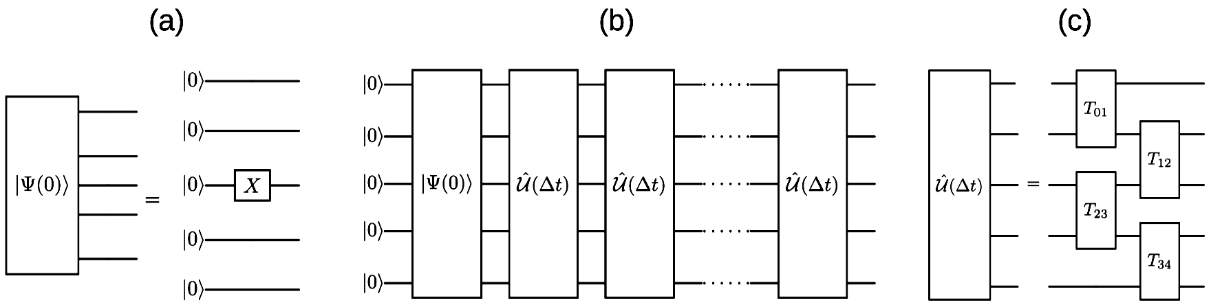
Figure 1: (a) The initial state $\ket{\psi(0)}=\ket{00100}$ in a 5-qubit system is prepared by applying NOT gate at third qubit. (b) The time evolution operator $\hat{U}$ is discretized into discrete steps and applied to the initial state (c) The discrete unitary operators $\hat{U}(\Delta t)$ are decomposed using basic trotterization.

Our simulation approach involves the following procedural stages:

1. Initialization: The initial state is generated by applying NOT gate(s) to the default state of the qubits on the IBM machine. For example, to create the state $\ket{\psi(0)}=\ket{00100}$ on a 5-qubit system, a NOT gate is applied to the third qubit, as shown in Fig. 1(a).

2. Time Discretization: To implement the time evolution operator $\hat{U}$ on the initial state $\ket{\psi(0)}$ in the IBM machine, we discretized time ($t$), expressing the evolution operator as the product of discrete time steps ($\Delta t$) -

   $$\hat{U}(t)=\hat{U}(\Delta t)\hat{U}(\Delta t)\dots\hat{U}(\Delta t).$$ (5)

   An associated diagram is provided in Fig. 1(b).

3. Trotterization: The discrete unitary operators $\hat{U}(\Delta t)$ undergo trotterization into a product of one and two-qubit unitaries ($T_{ij}$). In this study, we have utilized a basic trotterization method, as detailed in Appendix-B. The corresponding decomposition can be visualized in Fig. 1(c).

4. Gate Decomposition: The unitary ($T_{ij}$) is decomposed into CNOT and single-qubit rotation gates, suitable for direct application on IBM devices has been given in Ref. [86, 87, 57] and is shown in Fig. 2.

   

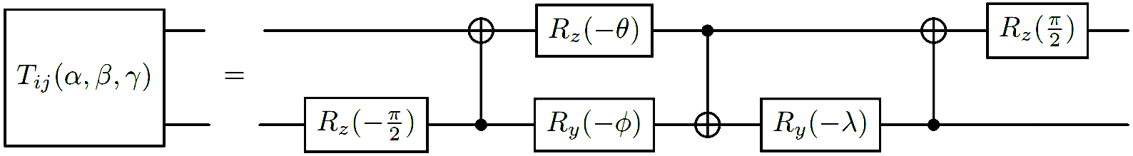
   Figure 2: The quantum circuit corresponding to the unitary operator, $T_{ij}(\alpha,\beta,\gamma)=exp[-i(\alpha\hat{\sigma}^{x}_{i}\hat{\sigma}^{x}_{j}+\beta\hat{\sigma}^{y}_{i}\hat{\sigma}^{y}_{j}+\gamma\hat{\sigma}^{z}_{i}\hat{\sigma}^{z}_{j})]$. Here, $\theta=\frac{\pi}{2}-2\gamma$, $\phi=2\alpha-\frac{\pi}{2}$ and $\lambda=\frac{\pi}{2}-2\beta$.

5. Measurement and Analysis: Subsequent to the evolution process, measurements in the computational basis are performed to obtain the state $\ket{\psi(t)}$. The dynamical quantity of interest, as defined in Eq. 3, is expressed as -

   $$n_{i}(t)=\langle\psi(t)|\hat{\sigma}^{z}_{i}|\psi(t)\rangle.$$ (6)

These steps collectively form the basis of our simulation approach, enabling the analysis of quantum walk in the chosen Fock state representation.

Quantum simulation on IBM quantum computers

In this report, we demonstrate outcomes derived from simulations conducted on the 127-qubit IBM "ibm_brisbane" instance. To benchmark our simulations, we compare the results with those obtained from an ideal Qasm-simulator ("Q-sim") and exact calculation ("Exact"). To address potential errors, we have also implemented readout error mitigation (REM) using the Qiskit runtime at optimization level 2. It is crucial to acknowledge that IBM machines undergo recalibration on a daily basis, introducing potential variations in data across different days. To address this, we examine some of the important analyses on the 7-qubit IBM instance "ibm_oslo" device, incorporating readout error mitigation techniques, as detailed in Appendix C. This approach aggregates data collected at various times and days, enhancing the robustness and inclusivity of our analysis. Moreover, we observed qualitative reproducibility, highlighting the reliability of our findings across various IBM machines. To tackle challenges arising from the reduced fidelity of two-qubit gates and potential errors due to extended execution times, we adopt a linear topology (with the optimization level set at 2) and implement basic trotterization up to 10 steps. The choice of a linear topology is crucial to ensure accurate simulation with superconducting qubits, aiming to avoid the requirement of SWAP operations.

Results

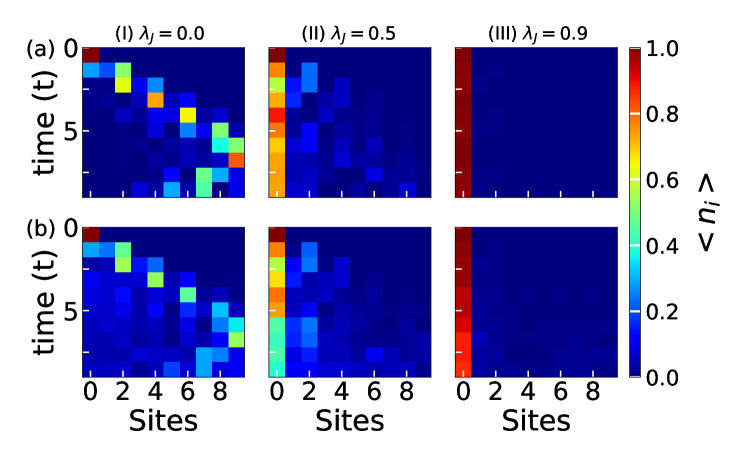
Figure 3: The figure depicts the density evolution of quantum walkers initialized with the state $\ket{\psi}_{I}=\hat{c}^{\dagger}_{0}\ket{vac}$. Panels (a) and (b) showcase results from "Q-sim" and readout error mitigated "ibm_brisbane," respectively. Figures (I), (II), and (III) correspond to amplitude modulations of $\lambda_{J}=0.1$, $0.5$, and $0.9$, respectively. Here, we consider $\phi_{J}=0$ and $L=10$.

Single-Particle Results. In this section, we investigate the single-particle quantum walk within the framework of the off-diagonal Aubry-André-Harper (AAH) model with quasiperiodic modulation, characterized by the Hamiltonian defined in Eq. 4. We have studied quantum walk on a system with $L$ lattice sites, equivalent to "$L$" qubits, by considering three initial states, which are given by -

$$\ket{\psi}_{I}=\hat{c}^{\dagger}_{0}\ket{vac},$$ (7)

where the particle resides at the left edge,

$$\ket{\psi}_{II}=\hat{c}^{\dagger}_{L}\ket{vac},$$ (8)

with the particle positioned at the right edge of the lattice and

$$\ket{\psi}_{III}=\hat{c}^{\dagger}_{L/2}\ket{vac},$$ (9)

where the particle is situated in the bulk of the system and $\ket{vac}$ is the empty state.

We initiate our investigation by setting the phase factor, denoted as $\phi_{J}$, to zero. Following this, we proceed to study the temporal evolution of the initial state $\ket{\psi}_{I}$ under the Hamiltonian, as specified in Equation 4. The dynamical evolutions are conducted both in the Q-sim and on the IBM machine, considering three distinct values of the hopping modulation strengths, namely $\lambda_{J}=0.0,0.5,\text{ and }0.9$ and the corresponding results are depicted in Figure 3(I)-(III). For $\lambda_{J}=0.0$, the walker undergoes a unidirectional quantum walk characterized by light-cone-like spreading reflects upon reaching the boundaries, as illustrated in Fig. 3a(I). As $\lambda_{J}$ increases, the walker gradually start to localize at the edge of the lattice. While in the case of large $\lambda_{J}$, complete localization is observed at the edge, as depicted in Fig. 3a(III). This distinctive localization behavior is attributed to the emergence of a topologically protected edge state, discussed in references [79, 41]. It is crucial to emphasize that analogous phenomena are evident in IBM machines, as exemplified in Panel-b of Fig. 3. Here, notable errors arise from trotter errors and inherent inaccuracies within the system after a few steps. It is important to note that, in accordance with the fundamental concepts of bulk-edge correspondence, this edge state consistently manifests across a range of periodic modulation strengths [79, 41]. Nevertheless, it is essential to note that in the quantum walk, the walker’s localization behaviour is less pronounced for weak modulation strengths. To quantify this, we have plotted the density at the first site, $P_{0}=\langle\hat{n}_{0}\rangle$ as a function of the modulation strengths, $\lambda_{J}$ at time, $t=5J^{-1}$, as shown in Fig. 5. The plot clearly indicates that edge localization gradual increase with an increase in modulation strength. Notably, IBM machine results align well with exact results, especially for larger $\lambda_{J}$ values, demonstrating improved accuracy. This amplitude modulation is also crucial for studying quantum information dynamics, enabling the control of information spread and speed via the amplitude parameter.

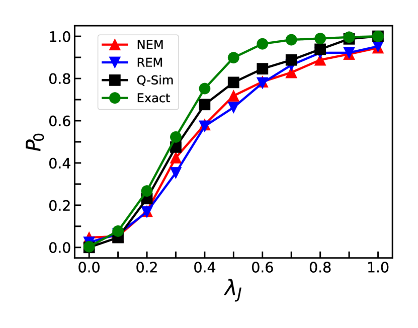
Figure 4: The figure displays $P_{0}$ at time $t=5J^{-1}$ for various $\lambda_{J}$ values, considering $\phi_{J}=0$. The data includes both No Error Mitigation (NEM) and Readout Error Mitigation (REM) data obtained from the "ibm_brisbane" machine.

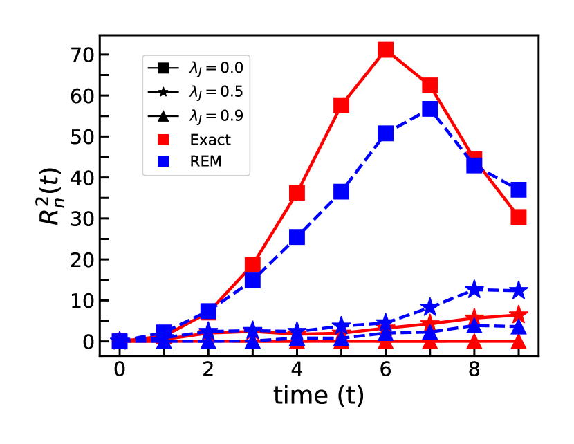
Figure 5: The figure displays $R_{n}^{2}(t)$ over time, t, for $\lambda_{J}=0.0,0.5$, and $0.9$. In this context, $\phi_{J}=0$. The data labeled REM corresponds to Readout Error Mitigation data obtained from the "ibm_brisbane" machine.

It’s important to highlight that, the density evolutions in the IBM machine deviate significantly from the exact ones for small $\lambda_{J}$ due to utilization of the basic trotterization with large step size. When $\lambda_{J}$ value become large, the impact of topological edge localization compensates for this error, resulting in more accurate results consistent with the exact dynamics. This consideration guides our preference for a larger step size in our study. To quantify this observations, we have computed the density-dependent radial distribution, denoted as $R_{n}^{2}(t)=\sum_{i}in_{i}(t)$, and depicted it in Fig. 5. Notably, for $\lambda_{J}=0.0$, the IBM machine result (square dashed line) significantly diverges from the exact result (square solid line) over time. However, as the values of $\lambda_{J}$ increase, the discrepancy diminishes over numerous steps. This emphasizes the significance of topological edge effects in compensating for trotter, gate and inherent system errors, thereby enhancing the reliability of our quantum walk simulations.

Figure 6: The figure illustrates the density evolution of quantum walkers initiated with the state $\ket{\psi}_{I}=\hat{c}^{\dagger}_{0}\ket{vac}$. Panels (a) and (b) present results from the "Q-sim" and readout error mitigated "ibm_oslo", respectively. Here we consider $\lambda_{J}=0.9$ and and $L=5$.

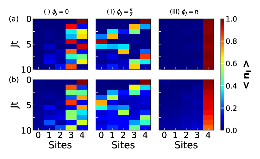
Figure 7: The figure illustrates the density evolution of quantum walkers initiated with the state $\ket{\psi}_{II}=\hat{c}^{\dagger}_{4}\ket{vac}$. Panels (a) and (b) present results from "Q-sim" and readout error mitigated "ibm_oslo", respectively. Here we consider $\lambda_{J}=0.9$ and and $L=5$.

Subsequently, we study the essential role of the phase factor in edge dynamics, utilizing the 7-qubit IBM machine "ibm_oslo" for density evolution under various phase conditions. In the case of the initial state $|\psi_{I}\rangle$, a pronounced left-edge localization is observed at $\phi=0$ (Fig. 7(I)), while the localization phenomenon diminishes for other $\phi$ values (Fig. 7(II-III)). Similarly, for initial state $|\psi_{III}\rangle$, right-edge localization emerges at $\phi=\pi$ (Fig. 7(III)), with the localization effect fading for other $\phi$ values (Fig. 7(I-II)). It is important to note that when an even system size considered, there are two edge states present only for $\phi=0$ (see Fig. 10(II)). For other values of $\phi$, edge states are not observed in the system (not shown). Note that, when the system size is odd, the phase factor shifts the edge state from one edge to the other, a phenomenon absent in even-numbered systems. Therefore, the phase factor holds paramount significance in topological quantum systems due to its susceptibility to specific conditions. This phase factor’s role in shaping quantum system behavior, particularly in determining edge state emergence, is crucial for various quantum information processing applications, significantly impacting algorithm and protocol development.

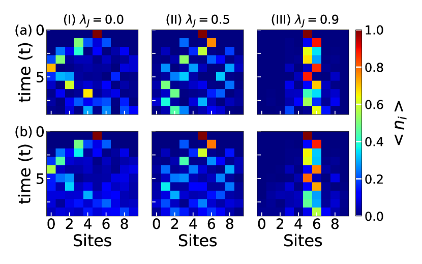
Figure 8: The figure displays the density evolution of quantum walkers initiated with the state $\ket{\psi}_{III}=\hat{c}^{\dagger}_{5}\ket{vac}$. Panels (a) and (b) depict results from the "Q-sim" and Readout Error Mitigation (REM) on the "ibm_brisbane," respectively. Here we consider $\phi_{J}=0$ and and $L=10$.

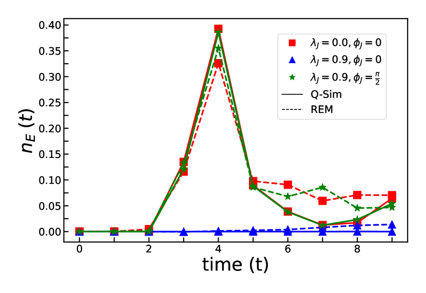
Figure 9: The illustrates $n_{E}(t)$ over time, $t$, with different $\lambda_{J}$ and $\phi_{J}$ values. The data includes results from "Q-sim" and Readout Error Mitigation (REM) on the "ibm_brisbane" machine. Here we consider $L=10$.

We further explore the quantum walk initiated from the bulk of the lattice. In Fig. 9, we illustrate the density evolution of the walker by initializing the quantum walk with the state defined by Eq. 8 for hopping modulation strengths, $\lambda_{J}=0.0,0.5,$ and $0.9$. In all instances, we set the phase factor, $\phi_{J}=0$. Notably, no localization phenomena are observed as the walker undergoes quantum walk from the lattice’s bulk. For $\lambda_{J}=0.0$, the walker exhibits ballistic spreading with a unidirectional bias owing to the basic trotterization. With an increase in $\lambda_{J}$, the walker’s spreading is progressively suppressed as depicted in Fig. 9(II) and (III) for $\lambda_{J}=0.5$ and $0.9$, respectively. Upon meticulous examination, it becomes evident that the population density of the walker at the lattice edges gradually decreases with an increase in the hopping modulation strength, ultimately vanishing at $\lambda_{J}=0.9$. We have chosen $L=10$, to facilitate the observation of two edge states. This behaviour is quantified by plotting the edge density, $n_{E}(t)=\frac{n_{0}(t)+n_{9}(t)}{2}$ as a function of time, $t$, as depicted in Fig. 9. For $\lambda_{J}=0$, the walker reaches the boundary, as evidenced by the peak in $n_{E}$ ( red square lines in Fig. 9). In contrast, at $\lambda_{J}=0.9$, $n_{E}(t)$ tends to zero (see up triangular blue lines in Fig. 9) indicates that the walker fails to reach the lattice boundaries $-$ an intriguing repulsion effect attributed to the presence of topologically protected edge states. This repulsion effect has an alternative interpretation within the context of the energy spectrum discussed in Ref [79]. The isolation of the zero-energy edge state from continuous or scattering states acts as a barrier for the particle initiating quantum walks from the bulk (edge) of the lattice, preventing them from accessing the edge (bulk) of the lattice sites. When the phase factor $\phi_{J}\neq 0$, the topological effect vanishes even for $\lambda_{J}=0.9$, enabling the walker to reach the lattice edges (similar to case of $\lambda_{J}=0$) without exhibiting a repulsion effect from the edge states (see green star lines in Fig. 9).

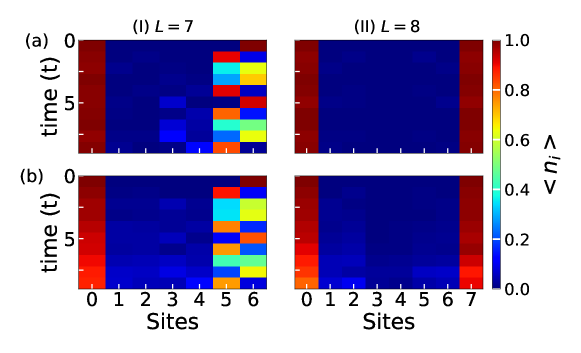
Figure 10: Figures (I) and (II) depicts the density evolution of quantum walkers initialized with the state $\ket{\psi}=\hat{c}^{\dagger}_{0}\hat{c}^{\dagger}_{6}\ket{vac}$ and $\ket{\psi}=\hat{c}^{\dagger}_{0}\hat{c}^{\dagger}_{7}\ket{vac}$, respectively. Panels (a) and (b) showcase results from "Q-sim" and readout error mitigated (REM) "ibm_brisbane," respectively. Here, we consider $\lambda_{J}=0.9$ and $\phi_{J}=0$.

Two-particle results. In this section, we investigate the quantum walk of two particles placed at the opposite ends of the lattice sites. We already discuss the single particle edge state along with different phase factors in the previous section. In this study, we set the phase factor $\phi_{J}$ = 0 and the hopping modulation strength $\lambda_{J}$ = 0.9, examining edge dynamics for both an odd and even number of lattice sites. The dynamics reveal the emergence of a single edge state for $L=7$ and two edge states for $L=8$, as shown in Fig. 7. This parity effect stems from the chiral symmetry inherent in the Hamiltonian [79]. Again this parity effect, indicating the emergence of single or multiple edge states based on lattice size, underscores the intricate interplay between system parameters and symmetries. This understanding informs the development of robust quantum algorithms and protocols while enhancing the fault tolerance of topological quantum computation, promising more reliable and stable quantum computing technologies [88].

Figure 11: The figure depicts the density evolution of quantum walkers initialized with the state $\ket{\psi}=\hat{c}^{\dagger}_{0}\hat{c}^{\dagger}_{3}\ket{vac}$. Panels (a) and (b) showcase results from "Q-sim" and readout error mitigated (REM) "ibm_brisbane," respectively. Figures (I), (II), and (III) correspond to $V=0$, $1$, and $2$, respectively. Here, we consider $L=7$, $\lambda_{J}=0.9$ and $\phi_{J}=0$.

Subsequently, we study the influence of interaction in the quantum walk, considering the initial state $|\psi\rangle=a_{0}a_{3}|0\rangle$, as illustrated in Fig. 11 for different interaction strengths. In this case, we set the hopping modulation strength $\lambda_{J}=0.9$ and the lattice size $L=7$ to induce the topological effect at one of the lattice edges. In the absence of interaction ($V=0$), the walker starting from the bulk can reach the boundary and interact with the edge walker, as illustrated in Fig. 11(I). However, with an increase in the interaction strength ($V=1$), the bulk walker experiences reflection from the edge walker, as depicted in Fig. 11(III). Further increasing the interaction strength ($V=2$), the bulk walker is unable to approach the edge walker, demonstrating a notable repulsion effect from the edge state in the presence of interaction. This repulsion effect has significant implications for quantum information dynamics, providing precise control over the transmission of two independent information. Tuning the interaction strength allows interference-free quantum communication, enabling the transmission of information along distinct paths without compromising signal integrity. This advancement has the potential to enhance controlled quantum communication protocols, contributing to improved reliability and efficiency in quantum information processing.

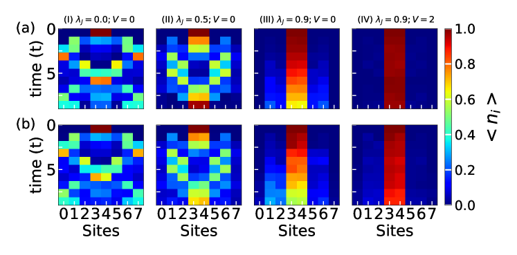
Figure 12: The figure shows the density evolution of quantum walkers initialized with the state $\ket{\psi}_{I}=\hat{c}^{\dagger}_{3}\hat{c}^{\dagger}_{4}\ket{vac}$. Panels (a) and (b) showcase results from "Q-sim" and readout error mitigated "ibm_brisbane," respectively. Here, we consider $L=8$ and $\phi_{J}=0$.

Next, we also investigate the quantum walk dynamics of two interacting particles situated within the lattice bulk, with the corresponding initial state denoted as $|\psi\rangle=a_{3}a_{4}|0\rangle$. Initially, we vary the hopping modulation strength while setting $V=0$ and $\phi_{J}=0$ , as shown in Fig. 12(I-III). For $\lambda_{J}=0$, the two walkers undergo independent particle quantum walks without affecting each others. Upon increasing $\lambda_{J}$, the walker spreading is gradually suppressed, and at $\lambda_{J}=0.9$, the two particles exhibit a collective behavior, moving as a composite particle with significantly slow spreading. Upon introducing nearest-neighbor interaction ($V$) into the system, an intriguing phenomenon emerges. For $\lambda_{J}=0.9$, a complete localization or the formation of a two-particle nearest-neighbour bound state occurs in the bulk of the system, as illustrated in Fig. 12(IV) for $V=2$. It is important to note that the formation of this bound state depends on specific bonds between lattice sites, especially those where the effective hopping strength is minimal (see Fig. 13(a)). If the two particles are positioned in different bonds or alternative locations within the bulk, the bound state does not occur solely with nearest-neighbor interaction strength. Additionally, in the presence of the phase factor, the bound state will not form, resulting in no localization phenomena in the dynamics except for $\phi_{J}=\pi$. This is because, for $\phi_{J}=\pi$, the lattice becomes identical to when $\phi_{J}=0$, except for altered effective hopping strengths in the bonds (see Fig. 13(b)).

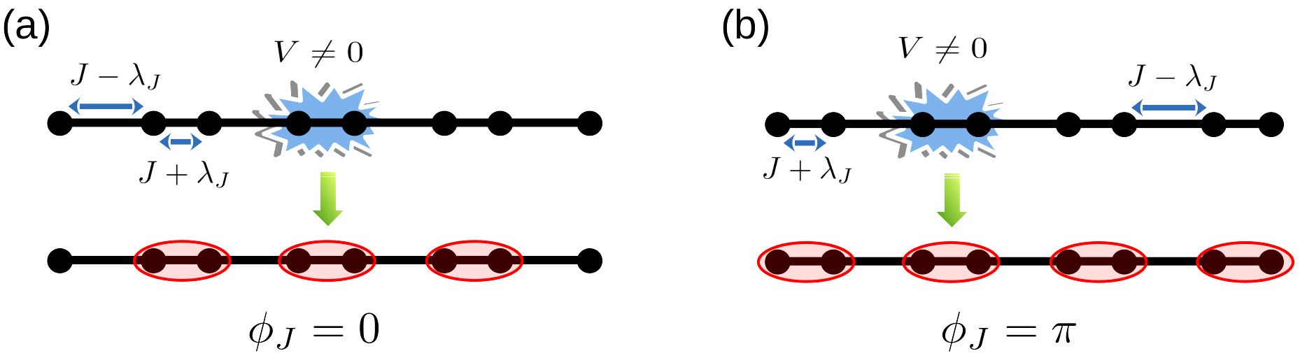
Figure 13: (a) and (b) correspond to the pictorial representation of the lattice for the phase factors $\phi_{J}=0$ and $\pi$, respectively. The red shaded region indicates the bonds where nearest-neighbor bound states are formed.

We further quantify this phenomena by calculating two-particle quantum correlation defined as-

$$C_{ij}(t)=\braket{\psi(t)}{\sigma^{z}_{i}}{\psi(t)}\braket{\psi(t)}{\sigma^{z}_{j}}{\psi(t)},$$ (10)

and plot it at time, $t=3J^{-1}$ in Fig. 14. It vividly exhibit the anti-bunching phenomenon, where the two-particle probabilities are distributed on both sides of the diagonal of the correlation matrix, indicating the fermionization of the two particles. When $V=0$, two particles symmetrically spread from the center for $\lambda_{J}=0$, resulting in symmetric bright spots at the anti-diagonal edges on the correlation matrix, indicating uniform expansion of the walker (see Fig. 14a(I)). With increasing $\lambda_{J}$, the walker expansion suppressed, causing correlations at the edges start to vanish and more concentrate at the center signifies the co-walking of the two particles (see Fig. 14a(II) and (III). When $V=2$ and $\lambda_{J}=0.9$, two particles become completely localized at the nearest-neighbor sites, forming a nearest-neighbour bound state and resulting in two nearest-neighbour bright patches on the both side of the diagonal of the correlation plot (see Fig. 14a(IV)). This bound state formation in the interacting off-diagonal Aubry-André-Harper model, facilitated by hopping modulation and nearest-neighbor interaction, has not been studied yet. In Panel-b of Fig. Fig. 14, correlations calculated using IBM machine data exhibit qualitative agreement with the Q-sim results .

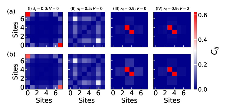
Figure 14: The figure shows the two-particle correlation, $C_{ij}$ for the initial state $\ket{\psi}_{I}=\hat{c}^{\dagger}_{3}\hat{c}^{\dagger}_{4}\ket{vac}$ at time, $t=3j^{-1}$. Panels (a) and (b) showcase results from "Q-sim" and readout error mitigated "ibm_brisbane," respectively. Here, we consider $L=8$ and $\phi_{J}=0$.

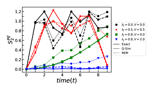
Figure 15: The figure depicts the participation entropy, $S_{2}^{PE}(t)$ as a function of time for the initial state $\ket{\psi}=\hat{c}^{\dagger}_{3}\hat{c}^{\dagger}_{4}\ket{vac}$. Here, we consider $L=8$ and $\phi_{J}=0$.

This bulk localization in the dynamics also can be further analyzed by the participation entropy as a function of time  [43] and is define as -

$$\centering S_{k}^{PE}(t)=\frac{1}{1-k}log(\frac{1}{N}\sum_{i=0}^{L-1}p_{i}(t)^{k}),\@add@centering$$ (11)

where $p_{i}(t)$ is the probability of the walker at site $i$ at time $t$, $k$ is the order of entropy and $N$ is the total number of particles in the system. In this report, we focus only on the second-order $(k=2)$ participation entropy, i.e., $S_{2}^{PE}(t)=-log[\frac{1}{N}\sum_{i=0}^{L-1}p_{i}(t)^{2}]$ and plot it as a function of time for different $\lambda_{J}$ and $V$ values in Fig. 15. First we consider $V=0$, the time evolution of the participation entropy increases along with oscillation after fast relaxation for $\lambda_{J}=0$. On increasing the $\lambda_{J}$, the participation entropy still oscillates but at smaller value and for $\lambda_{J}=0.9$, the participation entropy is suppressed significantly reflecting a localization phenomena in the system. Next on introducing $V$, the two particles forms a nearest-neighbour bound state, as a result participation entropy shows almost a flat line indicating there are no spreading in the bulk of the system. But in the NISQ IBM machine, we can see some spreading in the dynamics due to many effects from qubit noise to trotter error, still one can qualitatively study this off-diagonal AAH model due to its robust nature for $\lambda_{J}=0.9$. The observed phenomena of bulk localization in the presence of interaction bear substantial importance in the study of quantum many-body dynamics, quantum computation, and quantum information dynamics.

Conclusions

We have studied the quantum walk in the off-diagonal Aubrey-André model with quasi-periodic modulation (period $T=2$) at both single and two-particle levels. By considering different initial state, we have analyzed the impact of hopping modulation, phase factors and interaction on the quantum walk of single and two particles. We have initiated the quantum walk with a particle placed at the lattice edge, and the hopping modulation strength is systematically varied. We observed that the edge state becomes apparent when the hopping modulation is strong enough. The robustness of this edge state becomes evident as it exhibits resilience against factors such as qubit noise, trotter error and so on. This resilience is quantified through the analysis of the density-dependent radial distribution, and its reliability is further confirmed by comparisons with exact calculations. Furthermore, we investigated the impact of the phase factor on edge dynamics and observed that it significantly affects the position of the edge state, especially for odd-sized systems. Moreover, our investigation extended to the quantum walk initiated from the bulk of the system and we have obtained a repulsion effect from the edge state in the QW under sufficiently strong hopping modulation. We have also discussed the potential applications of the single-particle quantum walk in this system within the realm of quantum information dynamics. Subsequently, we have investigated the chiral nature of the off-diagonal AAH Hamiltonian in the quantum walk, observing distinct edge states based on the system’s parity. In addition, we also studied the interplay of interaction and topology, where the QW exhibit a repulsion effect from the topological edge state. This phenomenon, showcased in controlled quantum walk dynamics, suggests possibilities for interference-free quantum communication. In addition, we examine the quantum walk of two interacting particles in the lattice bulk, revealing a dynamics arising from hopping modulation and nearest-neighbor interaction, leading to the formation of the bound states. Studying this unfamiliar aspect enhances our understanding of the physics of the AAH model, which has profound implications for quantum many-body dynamics, quantum computation, and quantum information dynamics.

Appendix-A: Jordan-Wigner Transformation

The Jordan-Wigner transformation is a mathematical technique used in condensed matter physics to map the spin degrees of freedom of a one-dimensional system of electrons onto the fermionic degrees of freedom of a chain of non-interacting spinless fermions. This technique used in quantum computing to map the creation and annihilation operators of a spin system to a set of qubits. The creation and annihilation operators for a spin-1/2 system can be written in terms of the Pauli matrices, which are commonly used in quantum computation.

The Pauli matrices are defined as:

$$\begin{split}\sigma_{x}&=\ket{0}\bra{1}+\ket{1}\bra{0}\\ \sigma_{y}&=-i\ket{0}\bra{1}+i\ket{1}\bra{0}\\ \sigma_{z}&=\ket{0}\bra{0}-\ket{1}\bra{1}\end{split}$$ (12)

where $\ket{0}$ and $\ket{1}$ represent the two orthogonal basis states of a spin-1/2 system. Now the creation and annihilation operators are defined as:

$$\begin{split}\hat{c}^{\dagger}=\frac{\sigma_{x}-i\sigma_{y}}{2}=\sigma^{-}\;\;\;;\;\;\;\hat{c}=\frac{\sigma_{x}+i\sigma_{y}}{2}=\sigma^{+}\end{split}$$ (13)

Using these definitions, we can express the spin operators as linear combinations of the creation and annihilation operators:

$$\begin{split}S_{x}=\frac{\hat{c}^{\dagger}+\hat{c}}{2};\;\;\;\;\;\;S_{y}=\frac{\hat{c}^{\dagger}-\hat{c}}{2i};\;\;\;\;\;\;S_{z}=\frac{\hat{c}^{\dagger}\hat{c}-\hat{c}\hat{c}^{\dagger}}{2}\end{split}$$ (14)

where $S_{x}$, $S_{y}$, and $S_{z}$ are the Pauli spin operators.

But we also have to incorporate the anti-commutation relation of fermionic operators during the mapping and it is done by interspersing Z operators into the construction of the qubit operator which emulates the correct anti-commutation. For a 1D lattice with N sites, the corresponding transformation can be written as,

$$\begin{split}\hat{c}_{0}^{\dagger}&=\hat{\sigma}^{-}_{0}\otimes I_{1}\otimes I_{2}\dots I_{N}\\ \hat{c}_{1}^{\dagger}&={\sigma_{z}}_{0}\otimes\hat{\sigma}^{-}_{1}\otimes I_{2}\dots I_{N}\\ \vdots\\ {\hat{c}_{N}}^{\dagger}&={\sigma_{z}}_{0}\otimes{\sigma_{z}}_{1}\otimes{\sigma_{z}}_{2}\dots\otimes{\hat{\sigma}^{-}}_{N}\end{split}\quad\quad\quad\text{and}\quad\quad\quad\begin{split}\hat{c}_{0}&=\hat{\sigma}^{+}_{0}\otimes I_{1}\otimes I_{2}......I_{N}\\ {\hat{c}}_{1}&={{\sigma}_{z}}_{0}\otimes\hat{\sigma}^{+}_{1}\otimes I_{2}\dots I_{N}\\ \vdots\\ {\hat{c}}_{N}&={\sigma_{z}}_{0}\otimes{\sigma_{z}}_{1}\otimes{\sigma_{z}}_{2}\dots\otimes\hat{\sigma}^{+}_{N}.\end{split}$$ (15)

This transformation is known as Jordan-Wigner Transformation and $\otimes$ denotes the tensor product. Now any Hamiltonian under this transformation can be written as,

$$H=\sum_{i}h_{j}P_{j}=\sum_{i}h_{j}\Pi_{i}\sigma_{i}^{j}.$$ (16)

Where $h_{j}$ is the scalar coefficient and $P_{j}=\Pi_{i}\sigma_{i}^{j}$ ,where $\sigma_{i}^{j}$ is the Pauli matrices.

Here we have given a simple example of the Jordon-Wigner transformation. We consider a Bose-Hubbard Hamiltonian for a single particle in a one-dimensional lattice with $L=3$ lattice sites can be represented in terms of second quantized fermionic creation and annihilation operators.

$$H=-J(\hat{c}_{0}^{\dagger}\hat{c}_{1}+\hat{c}_{1}^{\dagger}\hat{c}_{0}+\hat{c}_{1}^{\dagger}\hat{c}_{2}+\hat{c}_{2}^{\dagger}\hat{c}_{1})$$ (17)

Now using Jordan Wigner transformation, we can rewrite the above Hamiltonian in terms of the product of Pauli matrices. The corresponding mapping is given below,

$$\begin{split}\hat{c}_{0}^{\dagger}&=\hat{\sigma}^{-}_{0}\otimes I_{1}\otimes I_{2}\\ {\hat{c}_{1}}^{\dagger}&={{\sigma}_{z}}_{0}\otimes\hat{\sigma}^{-}_{1}\otimes I_{2}\\ {\hat{c}_{2}}^{\dagger}&={{\sigma}_{z}}_{0}\otimes{{\sigma}_{z}}_{1}\otimes\hat{\sigma}^{-}_{2}\end{split}\quad\quad\quad\text{and}\quad\quad\quad\begin{split}\hat{c}_{0}&=\hat{\sigma}^{+}_{0}\otimes I_{1}\otimes I_{2}\\ {\hat{c}}_{1}&={\sigma_{z}}_{0}\otimes\hat{\sigma}^{+}_{1}\otimes I_{2}\\ {\hat{c}}_{2}&={\sigma_{z}}_{0}\otimes{\sigma_{z}}_{1}\otimes\hat{\sigma}^{+}_{2}.\end{split}$$ (18)

Now using the above relation and calculate the terms below as -

$$\begin{split}\hat{c}_{0}^{\dagger}\hat{c}_{1}+\hat{c}_{1}^{\dagger}\hat{c}_{0}&=(\hat{\sigma}^{-}_{0}\otimes I_{1}\otimes I_{2})({\sigma_{z}}_{0}\otimes\hat{\sigma}^{+}_{1}\otimes I_{2})+({\sigma_{z}}_{0}\otimes\hat{\sigma}^{-}_{1}\otimes I_{2})(\hat{\sigma}^{+}_{0}\otimes I_{1}\otimes I_{2})\\ &=(\hat{\sigma}^{-}_{0}{\sigma_{z}}_{0}\otimes\hat{\sigma}^{+}_{1}\otimes I_{2})+({\sigma_{z}}_{0}\hat{\sigma}^{+}_{0}\otimes\hat{\sigma}^{-}_{1}\otimes I_{2})\quad\text{[Using the relation: $(A\otimes B).(C\otimes D)=(A.C)\otimes(B.D)$]}\\ &=(\frac{{\sigma_{x}}_{0}-i{\sigma_{y}}_{0}}{2}){\sigma_{z}}_{0}\otimes(\frac{{\sigma_{x}}_{1}+i{\sigma_{y}}_{1}}{2})\otimes I_{2}+{\sigma_{z}}_{0}(\frac{{\sigma_{x}}_{0}+i{\sigma_{y}}_{0}}{2})\otimes(\frac{{\sigma_{x}}_{1}-i{\sigma_{y}}_{1}}{2})\otimes I_{2}\\ &=(\frac{{\sigma_{x}}_{0}-i{\sigma_{y}}_{0}}{2})\otimes(\frac{{\sigma_{x}}_{1}+i{\sigma_{y}}_{1}}{2})\otimes I_{2}+(\frac{{\sigma_{x}}_{0}+i{\sigma_{y}}_{0}}{2})\otimes(\frac{{\sigma_{x}}_{1}-i{\sigma_{y}}_{1}}{2})\otimes I_{2}\\ &=\frac{{\sigma_{x}}_{0}\otimes{\sigma_{x}}_{1}\otimes I_{2}}{2}+\frac{{\sigma_{y}}_{0}\otimes{\sigma_{y}}_{1}\otimes I_{2}}{2}\end{split}$$ (19)

Similarly, we get,

$${\hat{c}_{1}}^{\dagger}{\hat{c}}_{2}+{\hat{c}_{2}}^{\dagger}{\hat{c}}_{1}=\frac{I_{0}\otimes{\sigma_{x}}_{1}\otimes{\sigma_{x}}_{2}}{2}+\frac{I_{0}\otimes{\sigma_{y}}_{1}\otimes{\sigma_{y}}_{2}}{2}$$

Thus the Bose-Hubbard hamiltonian after Jordan-Wigner mapping will look like,

$$\hat{H}=-\frac{J}{2}({\sigma_{x}}_{0}\otimes{\sigma_{x}}_{1}\otimes I_{2}+{\sigma_{y}}_{0}\otimes{\sigma_{y}}_{1}\otimes I_{2}+I_{0}\otimes{\sigma_{x}1}_{1}\otimes{\sigma_{x}}_{2}+I_{0}\otimes{\sigma_{y}}_{1}\otimes{\sigma_{y}}_{2})$$ (20)

We remove the $\otimes$ and Identity from the above equation and rewrite the above Hamiltonian in a simple form as shown below

$$\hat{H}=-\frac{J}{2}\sum_{i=1}^{L-1}\sigma_{x}^{i}\sigma_{x}^{i+1}+\sigma_{y}^{i}\sigma_{y}^{i+1}$$ (21)

In this way, using Jordon-Wigner transformation fermionic operator can be easily mapped to Pauli spin operator, so that one can easily construct the quantum gates for quantum computations. But, in the case of bosonic systems, this transformation will not worked except for the hardcore limit, since in the hardcore limit Bose-Hubbard Hamiltonian equivalent to the spinless Fermi-Hubbard Hamiltonian.

Appendix-B: Suzuki-Trotter Decomposition

The Suzuki-Trotter decomposition is a technique used in quantum computing to simulate the evolution of a quantum system [89, 90]. The basic idea behind the Suzuki-Trotter decomposition is to break up the time evolution operator of a quantum system into a sequence of simpler operators that can be more easily simulated on a quantum computer. The decomposition is based on the Baker-Campbell-Hausdorff (BCH) formula, which expresses the product of two non-commuting operators as a sum of commutators. Consider a Hamiltonian containing only the local nearest neighbour interactions $h_{i}$’s can be written as

$$H=\sum_{i=1}^{L}h_{i}=\sum_{i\in odd}h_{i}+\sum_{i\in even}h_{i}=\hat{H}_{o}+\hat{H}_{e},$$ (22)

where $\hat{H}_{e}$ and $\hat{H}_{o}$ do not commute with each other. Then the exact time evolution operator becomes-

$$\hat{\mathcal{U}}(t)=e^{-{i\hat{H}t}}=e^{-{i(\hat{H}_{o}+\hat{H}_{e})t}}$$ (23)

Upon using the BCH formula the exact time evolution operator can be approximated as

$$\hat{\mathcal{U}}(t)\approx e^{-{i\hat{H}_{o}t}}e^{-{i\hat{H}_{e}t}}+\mathcal{O}(t^{2}).$$ (24)

This is known as first-order decomposition and error in each step is the order of $\mathcal{O}(t^{2})$. For a long time of evolution, we will break the evolution time $t$ into $n$ number of time steps or trotter steps of $\delta t(=t/n)$ duration. Then, time evolution can be approximated using the first-order Trotter decomposition formula is given by -

$$\hat{\mathcal{U}}(t)\approx(e^{-{i\hat{H}\delta t}})^{n}\approx(e^{-{i\hat{H}_{o}t/n}}e^{-{i\hat{H}_{e}t/n}})^{n}+\mathcal{O}(t^{2}/n).$$ (25)

We can see that for $n\rightarrow\infty$ i.e for large number of trotter steps or small time interval step $\delta t$, the unitary evolution becomes more accurate as shown below-

$$\hat{\mathcal{U}}(t)\approx\lim_{n\to\infty}(e^{-{i\hat{H}_{o}t/n}}e^{-{i\hat{H}_{e}t/n}})^{n}$$ (26)

The error in the first-order Suzuki-Trotter decomposition[91] can be further reduced by considering higher-order decomposition. For second-order decomposition one has to rewrite the time evolution as -

$$\hat{\mathcal{U}}(t)\approx e^{-{i\hat{H}_{o}t/2}}e^{-{i\hat{H}_{e}t}}e^{-{i\hat{H}_{o}t/2}}+\mathcal{O}(t^{3}),$$ (27)

here the error associated with each step is the order of $\mathcal{O}(t^{3})$. For $n$ step with step size of $\delta t=t/n$, the evolution operator becomes -

$$\hat{\mathcal{U}}(t)\approx(e^{-{i\hat{H}_{o}\delta t/2}}e^{-{i\hat{H}_{e}\delta t}}e^{-{i\hat{H}_{o}\delta t/2}})^{n}+\mathcal{O}(t^{3}/n^{2}).$$ (28)

The Suzuki-Trotter decomposition is widely used in quantum chemistry and condensed matter physics to simulate the behavior of complex quantum systems, and has been shown to be particularly effective for systems with strong interactions between particles. However, it should be noted that the accuracy of the method depends on the choice of the decomposition and the size of the time step, and may require some optimization for specific systems.

References

- [1] Aharonov, Y., Davidovich, L. & Zagury, N. Quantum random walks. \JournalTitlePhys. Rev. A 48, 1687–1690, DOI: 10.1103/PhysRevA.48.1687 (1993).
- [2] Childs, A. M., Farhi, E. & Gutmann, S. \JournalTitleQuantum Information Processing 1, 35–43, DOI: 10.1023/a:1019609420309 (2002).
- [3] Kempe, J. Quantum random walks: An introductory overview. \JournalTitleContemporary Physics 44, 307–327, DOI: 10.1080/00107151031000110776 (2003).
- [4] Venegas-Andraca, S. E. Quantum walks: a comprehensive review. \JournalTitleQuantum Information Processing 11, 1015–1106, DOI: 10.1007/s11128-012-0432-5 (2012).
- [5] Manouchehri, K. & Wang, J. Physical implementation of quantum walks. \JournalTitlePhysical Implementation of Quantum Walks, Springer DOI: 10.1007/978-3-642-36014-5 (2014).
- [6] Childs, A. M. & Goldstone, J. Spatial search by quantum walk. \JournalTitlePhys. Rev. A 70, 022314, DOI: 10.1103/PhysRevA.70.022314 (2004).
- [7] Ambainis, A. Quantum walks and their algorithmic applications. \JournalTitleInternational Journal of Quantum Information 1, 507–518 (2003).
- [8] Ambainis, A. Quantum walk algorithm for element distinctness. \JournalTitleSIAM Journal on Computing 37, 210–239, DOI: 10.1137/S0097539705447311 (2007). https://doi.org/10.1137/S0097539705447311.
- [9] Childs, A. M. & Ge, Y. Spatial search by continuous-time quantum walks on crystal lattices. \JournalTitlePhys. Rev. A 89, 052337, DOI: 10.1103/PhysRevA.89.052337 (2014).
- [10] Chakraborty, S., Novo, L., Ambainis, A. & Omar, Y. Spatial search by quantum walk is optimal for almost all graphs. \JournalTitlePhys. Rev. Lett. 116, 100501, DOI: 10.1103/PhysRevLett.116.100501 (2016).
- [11] Childs, A. M. Universal computation by quantum walk. \JournalTitlePhysical Review Letters 102, DOI: 10.1103/physrevlett.102.180501 (2009).
- [12] Childs, A. M., Gosset, D. & Webb, Z. Universal computation by multiparticle quantum walk. \JournalTitleScience 339, 791–794 (2013).
- [13] Zatelli, F., Benedetti, C. & Paris, M. G. A. Scattering as a quantum metrology problem: A quantum walk approach. \JournalTitleEntropy 22, DOI: 10.3390/e22111321 (2020).
- [14] Mohseni, M., Rebentrost, P., Lloyd, S. & Aspuru-Guzik, A. Environment-assisted quantum walks in photosynthetic energy transfer. \JournalTitleThe Journal of Chemical Physics 129, 174106, DOI: 10.1063/1.3002335 (2008).
- [15] Eisenberg, I. et al. Room temperature biological quantum random walk in phycocyanin nanowires. \JournalTitlePhysical Chemistry Chemical Physics 16, 11196–11201, DOI: 10.1039/C4CP00345D (2014).
- [16] Du, J. et al. Experimental implementation of the quantum random-walk algorithm. \JournalTitlePhys. Rev. A 67, 042316, DOI: 10.1103/PhysRevA.67.042316 (2003).
- [17] Ryan, C. A., Laforest, M., Boileau, J. C. & Laflamme, R. Experimental implementation of a discrete-time quantum random walk on an nmr quantum-information processor. \JournalTitlePhys. Rev. A 72, 062317, DOI: 10.1103/PhysRevA.72.062317 (2005).
- [18] Karski, M. et al. Quantum walk in position space with single optically trapped atoms. \JournalTitleScience 325, 174–177, DOI: 10.1126/science.1174436 (2009).
- [19] Schmitz, H. et al. Quantum walk of a trapped ion in phase space. \JournalTitlePhys. Rev. Lett. 103, 090504, DOI: 10.1103/PhysRevLett.103.090504 (2009).
- [20] Zähringer, F. et al. Realization of a quantum walk with one and two trapped ions. \JournalTitlePhys. Rev. Lett. 104, 100503, DOI: 10.1103/PhysRevLett.104.100503 (2010).
- [21] Preiss, P. M. et al. Strongly correlated quantum walks in optical lattices. \JournalTitleScience 347, 1229–1233, DOI: 10.1126/science.1260364 (2015).
- [22] Perets, H. B. et al. Realization of quantum walks with negligible decoherence in waveguide lattices. \JournalTitlePhys. Rev. Lett. 100, 170506, DOI: 10.1103/PhysRevLett.100.170506 (2008).
- [23] Peruzzo, A. et al. Quantum walks of correlated photons. \JournalTitleScience 329, 1500–1503, DOI: 10.1126/science.1193515 (2010).
- [24] Poulios, K. et al. Quantum walks of correlated photon pairs in two-dimensional waveguide arrays. \JournalTitlePhys. Rev. Lett. 112, 143604 (2014).
- [25] Yan, Z. et al. Strongly correlated quantum walks with a 12-qubit superconducting processor. \JournalTitleScience 364, 753–756, DOI: 10.1126/science.aaw1611 (2019).
- [26] Ye, Y. et al. Propagation and localization of collective excitations on a 24-qubit superconducting processor. \JournalTitlePhys. Rev. Lett. 123, 050502, DOI: 10.1103/PhysRevLett.123.050502 (2019).
- [27] Benedetti, C., Buscemi, F. & Bordone, P. Quantum correlations in continuous-time quantum walks of two indistinguishable particles. \JournalTitlePhys. Rev. A 85, 042314, DOI: 10.1103/PhysRevA.85.042314 (2012).
- [28] Qin, X. et al. Statistics-dependent quantum co-walking of two particles in one-dimensional lattices with nearest-neighbor interactions. \JournalTitlePhys. Rev. A 90, 062301 (2014).
- [29] Cai, X. et al. Multiparticle quantum walks and fisher information in one-dimensional lattices. \JournalTitlePhys. Rev. Lett. 127, 100406, DOI: 10.1103/PhysRevLett.127.100406 (2021).
- [30] Chandrashekar, C. M. Disordered-quantum-walk-induced localization of a bose-einstein condensate. \JournalTitlePhys. Rev. A 83, 022320, DOI: 10.1103/PhysRevA.83.022320 (2011).
- [31] Li, Z. J., Izaac, J. A. & Wang, J. B. Position-defect-induced reflection, trapping, transmission, and resonance in quantum walks. \JournalTitlePhys. Rev. A 87, 012314, DOI: 10.1103/PhysRevA.87.012314 (2013).
- [32] Mondal, S. & Mishra, T. Quantum walks of interacting mott-insulator defects with three-body interactions. \JournalTitlePhys. Rev. A 101, DOI: 10.1103/physreva.101.052341 (2020).
- [33] Lahini, Y. et al. Quantum walk of two interacting bosons. \JournalTitlePhys. Rev. A 86, 011603, DOI: 10.1103/PhysRevA.86.011603 (2012).
- [34] Wiater, D., Sowiński, T. & Zakrzewski, J. Two bosonic quantum walkers in one-dimensional optical lattices. \JournalTitlePhys. Rev. A 96, 043629, DOI: 10.1103/PhysRevA.96.043629 (2017).
- [35] Yalç ınkaya, i. d. I. & Gedik, Z. Two-dimensional quantum walk under artificial magnetic field. \JournalTitlePhys. Rev. A 92, 042324, DOI: 10.1103/PhysRevA.92.042324 (2015).
- [36] Razzoli, L., Paris, M. G. A. & Bordone, P. Continuous-time quantum walks on planar lattices and the role of the magnetic field. \JournalTitlePhys. Rev. A 101, 032336, DOI: 10.1103/PhysRevA.101.032336 (2020).
- [37] Joye, A. & Merkli, M. Dynamical localization of quantum walks in random environments. \JournalTitleJournal of Statistical Physics 140, 1025–1053, DOI: 10.1007/s10955-010-0047-0 (2010).
- [38] Shikano, Y. & Katsura, H. Localization and fractality in inhomogeneous quantum walks with self-duality. \JournalTitlePhys. Rev. E 82, 031122, DOI: 10.1103/PhysRevE.82.031122 (2010).
- [39] Kitagawa, T., Rudner, M. S., Berg, E. & Demler, E. Exploring topological phases with quantum walks. \JournalTitlePhys. Rev. A 82, 033429, DOI: 10.1103/PhysRevA.82.033429 (2010).
- [40] Asbóth, J. K. & Obuse, H. Bulk-boundary correspondence for chiral symmetric quantum walks. \JournalTitlePhys. Rev. B 88, 121406, DOI: 10.1103/PhysRevB.88.121406 (2013).
- [41] Wang, L., Liu, N., Chen, S. & Zhang, Y. Quantum walks in the commensurate off-diagonal aubry-andré-harper model. \JournalTitlePhys. Rev. A 95, 013619, DOI: 10.1103/PhysRevA.95.013619 (2017).
- [42] Zhang, J. et al. Observation of a many-body dynamical phase transition with a 53-qubit quantum simulator. \JournalTitleNature 551, 601–604, DOI: 10.1038/nature24654 (2017).
- [43] Li, H. et al. Observation of critical phase transition in a generalized aubry-andré-harper model with superconducting circuits. \JournalTitlenpj Quantum Information 9, 40, DOI: 10.1038/s41534-023-00712-w (2023).
- [44] Xie, D., Gou, W., Xiao, T., Gadway, B. & Yan, B. Topological characterizations of an extended su-schrieffer-heeger model. \JournalTitlenpj Quantum Information 5, 55, DOI: 10.1038/s41534-019-0159-6 (2019).
- [45] Xie, D. et al. Topological quantum walks in momentum space with a bose-einstein condensate. \JournalTitlePhys. Rev. Lett. 124, 050502, DOI: 10.1103/PhysRevLett.124.050502 (2020).
- [46] Tai, M. E. et al. Microscopy of the interacting harper–hofstadter model in the two-body limit. \JournalTitleNature 546, 519–523, DOI: 10.1038/nature22811 (2017).
- [47] Fukuhara, T. et al. Microscopic observation of magnon bound states and their dynamics. \JournalTitleNature 502, 76–79, DOI: 10.1038/nature12541 (2013).
- [48] Brydges, T. et al. Probing rényi entanglement entropy via randomized measurements. \JournalTitleScience 364, 260–263, DOI: 10.1126/science.aau4963 (2019). https://www.science.org/doi/pdf/10.1126/science.aau4963.
- [49] An, F. A., Meier, E. J. & Gadway, B. Engineering a flux-dependent mobility edge in disordered zigzag chains. \JournalTitlePhys. Rev. X 8, 031045, DOI: 10.1103/PhysRevX.8.031045 (2018).
- [50] Vovrosh, J. & Knolle, J. Confinement and entanglement dynamics on a digital quantum computer. \JournalTitleScientific Reports 11, 11577, DOI: 10.1038/s41598-021-90849-5 (2021).
- [51] Vijayan, J. et al. Time-resolved observation of spin-charge deconfinement in fermionic hubbard chains. \JournalTitleScience 367, 186, DOI: 10.1126/science.aay2354 (2020).
- [52] Aleksandrowicz, G. et al. Qiskit: An Open-source Framework for Quantum Computing, DOI: 10.5281/zenodo.2562111 (2019).
- [53] Pomarico, D. et al. Dynamical quantum phase transitions of the schwinger model: Real-time dynamics on ibm quantum. \JournalTitleEntropy 25, DOI: 10.3390/e25040608 (2023).
- [54] Zhukov, A. A., Remizov, S. V., Pogosov, W. V. & Lozovik, Y. E. Algorithmic simulation of far-from-equilibrium dynamics using quantum computer. \JournalTitleQuantum Information Processing 17, 223, DOI: 10.1007/s11128-018-2002-y (2018).
- [55] Cervera-Lierta, A. Exact Ising model simulation on a quantum computer. \JournalTitleQuantum 2, 114, DOI: 10.22331/q-2018-12-21-114 (2018).
- [56] Klco, N. et al. Quantum-classical computation of schwinger model dynamics using quantum computers. \JournalTitlePhys. Rev. A 98, 032331, DOI: 10.1103/PhysRevA.98.032331 (2018).
- [57] Smith, A., Kim, M. S., Pollmann, F. & Knolle, J. Simulating quantum many-body dynamics on a current digital quantum computer. \JournalTitlenpj Quantum Information 5, 106, DOI: 10.1038/s41534-019-0217-0 (2019).
- [58] Sabín, C. Digital quantum simulation of quantum gravitational entanglement with ibm quantum computers. \JournalTitleEPJ Quantum Technology 10, 4, DOI: 10.1140/epjqt/s40507-023-00161-6 (2023).
- [59] Nishi, H., Kosugi, T. & Matsushita, Y.-i. Implementation of quantum imaginary-time evolution method on nisq devices by introducing nonlocal approximation. \JournalTitlenpj Quantum Information 7, 85, DOI: 10.1038/s41534-021-00409-y (2021).
- [60] Kamakari, H., Sun, S.-N., Motta, M. & Minnich, A. J. Digital quantum simulation of open quantum systems using quantum imaginary–time evolution. \JournalTitlePRX Quantum 3, 010320, DOI: 10.1103/PRXQuantum.3.010320 (2022).
- [61] Sun, S.-N. et al. Quantum computation of finite-temperature static and dynamical properties of spin systems using quantum imaginary time evolution. \JournalTitlePRX Quantum 2, 010317, DOI: 10.1103/PRXQuantum.2.010317 (2021).
- [62] McCaskey, A. J. et al. Quantum chemistry as a benchmark for near-term quantum computers. \JournalTitlenpj Quantum Information 5, 99, DOI: 10.1038/s41534-019-0209-0 (2019).
- [63] O’Malley, P. J. J. et al. Scalable quantum simulation of molecular energies. \JournalTitlePhys. Rev. X 6, 031007, DOI: 10.1103/PhysRevX.6.031007 (2016).
- [64] Wang, Y., Li, Y., Yin, Z.-q. & Zeng, B. 16-qubit ibm universal quantum computer can be fully entangled. \JournalTitlenpj Quantum Information 4, 46, DOI: 10.1038/s41534-018-0095-x (2018).
- [65] Choo, K., von Keyserlingk, C. W., Regnault, N. & Neupert, T. Measurement of the entanglement spectrum of a symmetry-protected topological state using the ibm quantum computer. \JournalTitlePhys. Rev. Lett. 121, 086808, DOI: 10.1103/PhysRevLett.121.086808 (2018).
- [66] Harper, P. G. Single band motion of conduction electrons in a uniform magnetic field. \JournalTitleProceedings of the Physical Society. Section A 68, 874, DOI: 10.1088/0370-1298/68/10/304 (1955).
- [67] Aubry, S. & André, G. Analyticity breaking and Anderson localization in incommensurate lattices. Horwitz, L. P. (ed.) et al., Group theoretical methods in physics. Proceedings of the 8th international colloquium, Kiryat Anavim, Israel, March 25-29, 1979. Bristol: Adam Hilger. Ann. Isr. Phys. Soc. 3, 133-164 (1980). (1980).
- [68] Thouless, D. J. Bandwidths for a quasiperiodic tight-binding model. \JournalTitlePhys. Rev. B 28, 4272–4276, DOI: 10.1103/PhysRevB.28.4272 (1983).
- [69] Hiramoto, H. & Kohmoto, M. New localization in a quasiperiodic system. \JournalTitlePhys. Rev. Lett. 62, 2714–2717, DOI: 10.1103/PhysRevLett.62.2714 (1989).
- [70] Vidal, J., Mouhanna, D. & Giamarchi, T. Correlated fermions in a one-dimensional quasiperiodic potential. \JournalTitlePhys. Rev. Lett. 83, 3908–3911, DOI: 10.1103/PhysRevLett.83.3908 (1999).
- [71] Kraus, Y. E., Lahini, Y., Ringel, Z., Verbin, M. & Zilberberg, O. Topological states and adiabatic pumping in quasicrystals. \JournalTitlePhys. Rev. Lett. 109, 106402, DOI: 10.1103/PhysRevLett.109.106402 (2012).
- [72] Iyer, S., Oganesyan, V., Refael, G. & Huse, D. A. Many-body localization in a quasiperiodic system. \JournalTitlePhys. Rev. B 87, 134202, DOI: 10.1103/PhysRevB.87.134202 (2013).
- [73] Schreiber, M. et al. Observation of many-body localization of interacting fermions in a quasirandom optical lattice. \JournalTitleScience 349, 842–845, DOI: 10.1126/science.aaa7432 (2015). https://www.science.org/doi/pdf/10.1126/science.aaa7432.
- [74] Bordia, P., Lüschen, H., Schneider, U., Knap, M. & Bloch, I. Periodically driving a many-body localized quantum system. \JournalTitleNature Physics 13, 460–464, DOI: 10.1038/nphys4020 (2017).
- [75] Lahini, Y. et al. Observation of a localization transition in quasiperiodic photonic lattices. \JournalTitlePhys. Rev. Lett. 103, 013901, DOI: 10.1103/PhysRevLett.103.013901 (2009).
- [76] Shi, Y.-H. et al. Quantum simulation of topological zero modes on a 41-qubit superconducting processor. \JournalTitlePhys. Rev. Lett. 131, 080401, DOI: 10.1103/PhysRevLett.131.080401 (2023).
- [77] Chang, I., Ikezawa, K. & Kohmoto, M. Multifractal properties of the wave functions of the square-lattice tight-binding model with next-nearest-neighbor hopping in a magnetic field. \JournalTitlePhys. Rev. B 55, 12971–12975, DOI: 10.1103/PhysRevB.55.12971 (1997).
- [78] Wang, Y., Cheng, C., Liu, X.-J. & Yu, D. Many-body critical phase: Extended and nonthermal. \JournalTitlePhys. Rev. Lett. 126, 080602, DOI: 10.1103/PhysRevLett.126.080602 (2021).
- [79] Ganeshan, S., Sun, K. & Das Sarma, S. Topological zero-energy modes in gapless commensurate aubry-andré-harper models. \JournalTitlePhys. Rev. Lett. 110, 180403, DOI: 10.1103/PhysRevLett.110.180403 (2013).
- [80] Liu, F., Ghosh, S. & Chong, Y. D. Localization and adiabatic pumping in a generalized aubry-andré-harper model. \JournalTitlePhys. Rev. B 91, 014108, DOI: 10.1103/PhysRevB.91.014108 (2015).
- [81] Ke, Y. et al. Topological phase transitions and thouless pumping of light in photonic waveguide arrays. \JournalTitleLaser & Photonics Reviews 10, 995–1001, DOI: https://doi.org/10.1002/lpor.201600119 (2016).
- [82] Verbin, M., Zilberberg, O., Kraus, Y. E., Lahini, Y. & Silberberg, Y. Observation of topological phase transitions in photonic quasicrystals. \JournalTitlePhys. Rev. Lett. 110, 076403, DOI: 10.1103/PhysRevLett.110.076403 (2013).
- [83] An, F. A. et al. Interactions and mobility edges: Observing the generalized aubry-andré model. \JournalTitlePhys. Rev. Lett. 126, 040603, DOI: 10.1103/PhysRevLett.126.040603 (2021).
- [84] Yan, W. et al. Direct observation of anderson localization of ultracold atoms in a quasiperiodic lattice. \JournalTitleOpt. Continuum 2, 2116–2121, DOI: 10.1364/OPTCON.499768 (2023).
- [85] Xiao, T. et al. Observation of topological phase with critical localization in a quasi-periodic lattice. \JournalTitleScience Bulletin 66, 2175–2180, DOI: https://doi.org/10.1016/j.scib.2021.07.025 (2021).
- [86] Vatan, F. & Williams, C. Optimal quantum circuits for general two-qubit gates. \JournalTitlePhys. Rev. A 69, 032315, DOI: 10.1103/PhysRevA.69.032315 (2004).
- [87] Kraus, B. & Cirac, J. I. Optimal creation of entanglement using a two-qubit gate. \JournalTitlePhys. Rev. A 63, 062309, DOI: 10.1103/PhysRevA.63.062309 (2001).
- [88] Sarma, S. D., Freedman, M. & Nayak, C. Majorana zero modes and topological quantum computation. \JournalTitlenpj Quantum Information 1, 15001, DOI: 10.1038/npjqi.2015.1 (2015).
- [89] Hatano, N. & Suzuki, M. Finding Exponential Product Formulas of Higher Orders, 37–68 (Springer Berlin Heidelberg, Berlin, Heidelberg, 2005).
- [90] Daley, A. J. et al. Practical quantum advantage in quantum simulation. \JournalTitleNature 607, 667–676, DOI: 10.1038/s41586-022-04940-6 (2022).
- [91] Nielsen, M. A. & Chuang, I. L. Quantum Computation and Quantum Information: 10th Anniversary Edition (Cambridge University Press, 2011).