We extend the existing leading (LO), next-to-leading (NLO), and next-to-next-to-leading order (NNLO) NNPDF4.0 sets of parton distribution functions (PDFs) to approximate next-to-next-to-next-to-leading order (aN³LO). We construct an approximation to the N³LO splitting functions that includes all available partial information from both fixed-order computations and from small and large $x$ resummation, and estimate the uncertainty on this approximation by varying the set of basis functions used to construct the approximation. We include known N³LO corrections to deep-inelastic scattering structure functions and extend the FONLL general-mass scheme to $\mathcal{O}\left(\alpha_{s}^{3}\right)$ accuracy. We determine a set of aN³LO PDFs by accounting both for the uncertainty on splitting functions due to the incomplete knowledge of N³LO terms, and to the uncertainty related to missing higher corrections (MHOU), estimated by scale variation, through a theory covariance matrix formalism. We assess the perturbative stability of the resulting PDFs, we study the impact of MHOUs on them, and we compare our results to the aN³LO PDFs from the MSHT group. We examine the phenomenological impact of aN³LO corrections on parton luminosities at the LHC, and give a first assessment of the impact of aN³LO PDFs on the Higgs and Drell-Yan total production cross-sections. We find that the aN³LO NNPDF4.0 PDFs are consistent within uncertainties with their NNLO counterparts, that they improve the description of the global dataset and the perturbative convergence of Higgs and Drell-Yan cross-sections, and that MHOUs on PDFs decrease substantially with the increase of perturbative order.

1 Introduction

Calculations of hard-scattering cross-sections at fourth perturbative order in the strong coupling, i.e. at next-to-next-to-next-to-leading order (N³LO), have been available for a long time for massless deep-inelastic scattering (DIS) [1, 2, 3, 4], and have more recently become available for a rapidly growing set of hadron collider processes. These include inclusive Higgs production in gluon-fusion [5, 6], bottom-fusion [7], in association with vector bosons [8], and in vector-boson-fusion [9], Higgs pair production [10], inclusive Drell-Yan production [11, 12], differential Higgs production [13, 14, 15, 16, 17], and differential Drell-Yan distributions [18, 19], see [20] for an overview.

In order to obtain predictions for hadronic observables with this accuracy, these partonic cross-sections must be combined with parton distribution functions (PDFs) determined at the same perturbative order. These, in turn, must be determined by comparing to experimental data theory predictions computed at the same accuracy. The main bottleneck in carrying out this programme is the lack of exact expressions for the N³LO splitting functions that govern the scale dependence of the PDFs: for these only partial information is available [21, 22, 23, 24, 25, 26, 27, 28, 29, 30, 31]. This information includes a set of integer $N$-Mellin moments, terms proportional to $n_{f}^{k}$ with $k\geq 1$, and the large- and small-$x$ limits. By combining these partial results it is possible to attempt an approximate determination of the N³LO splitting functions [30, 32], as was successfully done in the past at NNLO [33].

At present a global PDF determination at N³LO must consequently be based on incomplete information: the approximate knowledge of splitting functions, and full knowledge of partonic cross-sections only for a subset of processes. A first attempt towards achieving this was recently made in Ref. [32], where the missing theoretical information on N³LO calculations was parametrized in terms of a set of nuisance parameters, which were determined together with the PDFs from a fit to experimental data.

Here we adopt a somewhat different strategy. Namely, we use a theory covariance matrix formalism in order to account for the missing perturbative information. It was shown in Ref. [34] that nuclear uncertainties can be included through a theory covariance matrix, and it was further shown in Refs. [35, 36] how such a theory covariance matrix can be constructed to account for missing higher-order uncertainties (MHOUs), estimated through renormalization and factorization scale variation. Here we will use the same formalism in order to also construct a theory covariance matrix for incomplete higher-order uncertainties (IHOUs), namely, those related to incomplete knowledge of the N³LO theory, specifically for the splitting functions and for the massive DIS coefficient functions. Equipped with such theory covariance matrices, we can perform a determination of PDFs at “approximate N³LO” (hereafter denoted aN³LO), in which the theory covariance matrix accounts both for incomplete knowledge of N³LO splitting functions and massive coefficient functions (IHOUs), and for missing N³LO corrections to the partonic cross-sections for hadronic processes (MHOUs).

We will thus present the aN³LO NNPDF4.0 PDF determination, to be added to the existing LO, NLO and NNLO sets [37], as well as the more recent NNPDF4.0 MHOU PDFs [38] that also include MHOUs in the PDF uncertainty. Besides using a different methodology to the MSHT20 study [32], here we are also able to include more recent exact results [28, 29, 30, 31] that stabilize the N³LO splitting function parametrisation. Our construction is implemented in the open-source NNPDF framework [39]. Specifically, our aN³LO evolution is implemented in EKO [40] and the N³LO DIS coefficient functions, including the FONLL general-mass scheme, in YADISM [41]. With PDFs determined from the same global dataset and using the same methodology at four consecutive perturbative orders it is now possible to assess carefully perturbative stability and provide a reliable uncertainty estimation.

The outline of this paper is as follows. In Sect. 2 we construct an approximation to the N³LO splitting functions based on all known exact results and limits. We compare it with the MSHT approximation [32] as well as with the more recent approximation of Refs. [28, 29, 30]. In Sect. 3 we discuss available and approximate N³LO corrections to hard cross sections: specifically, DIS coefficient functions, including a generalization to this order of the FONLL [42, 43, 44] method for the inclusion of heavy quark mass effects, and the Drell-Yan cross-section. In Sect. 4 we present the main results of this work, namely the aN³LO NNPDF4.0 PDF set, based on the results of Sects. 2 and 3. Perturbative convergence before and after the inclusion of MHOUs is discussed in detail, and results are compared to those of the MSHT group [32]. A first assessment of the impact of aN³LO PDFs on Drell-Yan and Higgs production is presented in Sect. 5. Finally, a summary and outlook on future developments are presented in Sect. 6. Expressions for the anomalous dimensions parametrized in Sects. 2.3-2.4 are given in Appendix A.

2 Approximate N³LO evolution

We proceed to the construction and implementation of aN³LO evolution. We first describe our strategy to approximate the N³LO evolution equations, the way this is used to construct aN³LO anomalous dimensions and splitting functions, and to estimate the uncertainty in the approximation and its impact on theory predictions. We then use this strategy to construct an approximation in the nonsinglet sector, where accurate results have been available for a while [22], and benchmark it against these results. We then present our construction of aN³LO singlet splitting functions, examine our results, their uncertainties and their perturbative behavior, and also how they relate to NLL small-$x$ resummation. We next describe our implementation of aN³LO evolution and study the impact of aN³LO on the perturbative evolution of PDFs. Finally, we compare our aN³LO singlet splitting functions to those of the MSHT group and to the recent results of [28, 29, 30].

2.1 Construction of the approximation

We write the QCD evolution equations as

$$\mu^{2}\frac{\partial f_{i}(x,\mu^{2})}{\partial\mu^{2}}=\int_{x}^{1}\frac{dz}{z}P_{ij}(x/z,a_{s}(\mu^{2}))f_{j}(z,\mu^{2})\,,$$ (2.1)

where $f_{i}(x,\mu^{2})$ is a vector of PDFs and, with $n_{f}$ active quark flavors, the $\left(2n_{f}+1\right)\times\left(2n_{f}+1\right)$ splitting function matrix $P_{ij}(x,a_{s}(\mu^{2}))$ is expanded perturbatively as

$$P_{ij}(x,a_{s}(\mu^{2}))=a_{s}P_{ij}^{(0)}(x)+a_{s}^{2}P_{ij}^{(1)}(x)+a_{s}^{3}P_{ij}^{(2)}(x)+a_{s}^{4}P_{ij}^{(3)}(x)+\mathcal{O}\left(a_{s}^{5}\right)\,.$$ (2.2)

in powers of the strong coupling $a_{s}(\mu^{2})=\alpha_{s}(\mu^{2})/4\pi$.

Defining Mellin space PDFs $f_{i}(N,\mu^{2})$ (denoted in a slight abuse of notation by the same symbol as the $x$-space PDFs), and anomalous dimensions $\gamma_{ij}(N,a_{s}(\mu^{2}))$ as minus the Mellin transforms of splitting functions,

$$f_{i}(N,\mu^{2}) =\mathcal{M}[f_{i}(x,\mu^{2})](N)=\int\limits_{0}^{1}dx\,x^{N-1}f_{i}(x,\mu^{2})$$ (2.3)

$$\gamma_{ij}(N,a_{s}(\mu^{2})) =-\mathcal{M}[P_{ij}(x,a_{s}(\mu^{2}))](N)=-\int\limits_{0}^{1}dx\,x^{N-1}P_{ij}(x,a_{s}(\mu^{2}))$$ (2.4)

the evolution equations become

$$\mu^{2}\frac{\partial f_{i}(N,\mu^{2})}{\partial\mu^{2}}=-\gamma_{ij}(N,a_{s}(\mu^{2}))f_{j}(N,\mu^{2})\,,$$ (2.5)

where the perturbative expansion of the anomalous dimensions is

$$\gamma_{ij}(N,a_{s}(\mu^{2}))=a_{s}\gamma_{ij}^{(0)}(N)+a_{s}^{2}\gamma_{ij}^{(1)}(N)+a_{s}^{3}\gamma_{ij}^{(2)}(N)+a_{s}^{4}\gamma_{ij}^{(3)}(N)+\mathcal{O}\left(a_{s}^{5}\right)\,.$$ (2.6)

The $\left(2n_{f}+1\right)\times\left(2n_{f}+1\right)$ matrix of anomalous dimensions has seven independent entries (see e.g. [45]), driving the evolution of various PDF combinations as follows:

• All nonsinglet combinations

  $$q^{\pm}_{ij} =q^{\pm}_{i}-\bar{q}^{\pm}_{j},$$ (2.7)

  $$\quad q^{\pm}_{i} =q_{i}\pm\bar{q}_{i}$$ (2.8)

  satisfy decoupled evolution equations with the same two anomalous dimension $\gamma_{{\rm ns},\pm}$; note that the plus and minus variants of $\gamma_{{\rm ns},\pm}$ start differing from each other already at NLO.

• The total valence combination

  $$V=\sum_{i=1}^{n_{f}}q^{-}_{i}$$ (2.9)

  satisfies a decoupled evolution equation with an anomalous dimension

  $$\gamma_{\rm ns,v}=\gamma_{\rm ns,s}+\gamma_{{\rm ns},-}\,;$$ (2.10)

  note that the flavor-independent “sea” contribution $\gamma_{\rm ns,s}$ starts being nonzero only at NNLO.

• The singlet combination

  $$\Sigma=\sum_{i=1}^{n_{f}}q_{i}^{+}$$ (2.11)

  mixes with the gluon

  $$\mu^{2}\frac{\partial}{\partial\mu^{2}}\begin{pmatrix}\Sigma(N,\mu^{2})\\ g(N,\mu^{2})\end{pmatrix}=-\begin{pmatrix}\gamma_{qq}(N,a_{s}(\mu^{2}))&\gamma_{qg}(N,a_{s}(\mu^{2}))\\ \gamma_{gq}(N,a_{s}(\mu^{2}))&\gamma_{gg}(N,a_{s}(\mu^{2}))\\ \end{pmatrix}\begin{pmatrix}\Sigma(N,\mu^{2})\\ g(N,\mu^{2})\end{pmatrix}\,.$$ (2.12)

  The quark-quark entry of the anomalous dimension matrix can be further decomposed into nonsinglet and pure singlet contributions according to

  $$\gamma_{qq}=\gamma_{{\rm ns},+}+\gamma_{{qq},{\rm ps}}\,,$$ (2.13)

  where the pure singlet contribution $\gamma_{{qq},{\rm ps}}$ starts at NLO.

There are thus seven independent contributions: three in the nonsinglet sector, $\gamma_{{\rm ns},\pm}$ and $\gamma_{\rm ns,s}$, and four in the singlet sector, $\gamma_{{qq},{\rm ps}}$, $\gamma_{{qg}}$, $\gamma_{{gq}}$, and $\gamma_{{gg}}$. In turn, each of these anomalous dimensions can be expanded according to Eq. (2.6). Our goal is to determine an approximate expression for the corresponding seven $\gamma_{ij}^{(3)}(N)$ N³LO terms.

The information that can be exploited in order to achieve this goal comes from three different sources: (1) full analytic knowledge of contributions to the anomalous dimensions proportional to the highest powers of the number of flavors $n_{f}$; (2) large-$x$ and small-$x$ resummations provide all-order information on terms that are logarithmically enhanced by powers of $\ln(1-x)$ and $\ln x$ respectively; (3) analytic knowledge of a finite set of integer moments. We construct an approximation based on this information by first separating off the analytically known terms (1-2), then expanding the remainder on a set of basis functions and using the known moments to determine the expansion coefficients. Finally, we vary the set of basis functions in order to obtain an estimate of the uncertainties.

Schematically, we proceed as follows:

1. We include all terms in the expansion

   $$\gamma_{ij}^{(3)}(N)=\gamma_{ij}^{(3,0)}(N)+n_{f}\gamma_{ij}^{(3,1)}(N)+n_{f}^{2}\gamma_{ij}^{(3,2)}(N)+n_{f}^{3}\gamma_{ij}^{(3,3)}(N)\,,$$ (2.14)

   of the anomalous dimension in powers of $n_{f}$ that are fully or partially known analytically. We collectively denote such terms as $\gamma_{ij,n_{f}}^{(3)}(N)$.

2. We include all terms from large-$x$ and small-$x$ resummation, to the highest known logarithmic accuracy, including all known subleading power corrections in both limits. We denote these terms as $\gamma_{ij,N\to\infty}^{(3)}(N)$ and $\gamma_{ij,N\to 0}^{(3)}(N)$, $\gamma_{ij,N\to 1}^{(3)}(N)$ respectively. Possible double counting coming from the overlap of these terms with $\gamma_{ij,n_{f}}^{(3)}(N)$ is removed.

3. We write the approximate anomalous dimension matrix element $\gamma_{ij}^{(3)}(N)$ as the sum of the terms which are known exactly and a remainder $\widetilde{\gamma}_{ij}^{(3)}(N)$ according to

   $$\gamma_{ij}^{(3)}(N)=\gamma_{ij,n_{f}}^{(3)}(N)+\gamma_{ij,N\to\infty}^{(3)}(N)+\gamma_{ij,N\to 0}^{(3)}(N)+\gamma_{ij,N\to 1}^{(3)}(N)+\widetilde{\gamma}_{ij}^{(3)}(N)\,.$$ (2.15)

   We determine the remainder as a linear combination of a set of $n^{ij}$ interpolating functions $G^{ij}_{\ell}(N)$ (kept fixed) and $H^{ij}_{\ell}(N)$ (to be varied)

   $$\widetilde{\gamma}_{ij}^{(3)}(N)=\sum_{\ell=1}^{n^{ij}-n_{H}}b^{ij}_{\ell}G^{ij}_{\ell}(N)+\sum_{\ell=1}^{n_{H}}b^{ij}_{n^{ij}-2+\ell}H^{ij}_{\ell}(N)\,,$$ (2.16)

   with $n^{ij}$ equal to the number of known Mellin moments of $\gamma_{ij}^{(3)}(N)$. We determine the coefficients $b^{ij}_{\ell}$ by equating the evaluation of $\widetilde{\gamma}_{ij}^{(3)}(N)$ to the known moments of the splitting functions.

4. In the singlet sector, we take $n_{H}=2$ and we make $\widetilde{N}_{ij}$ different choices for the two functions $H^{ij}_{\ell}(N)$, by selecting them out of a list of distinct basis functions (see Sect. 2.4 below). Thereby, we obtain $\widetilde{N}_{ij}$ expressions for the remainder $\widetilde{\gamma}_{ij}^{(3)}(N)$ and accordingly for the N³LO anomalous dimension matrix element ${\gamma}_{ij}^{(3)}(N)$ through Eq. (2.15). These are used to construct the approximate anomalous dimension matrix and the uncertainty on it, in the way discussed in Sect. 2.2 below. In the nonsinglet sector instead, we take $n_{H}=0$, i.e. we take a unique answer as our approximation, and we neglect the uncertainty on it, for reasons to be discussed in greater detail at the end of Sect. 2.3.

2.2 The approximate anomalous dimension matrix and its uncertainty

The procedure described in Sect. 2.1 provides us with an ensemble of $\widetilde{N}_{ij}$ different approximations to the N³LO anomalous dimension, denoted $\gamma_{ij}^{(3),\,(k)}(N)$, $k=1,\dots\widetilde{N}_{ij}$ . Our best estimate for the approximate anomalous dimension is then their average

$$\gamma_{ij}^{(3)}(N)=\frac{1}{\widetilde{N}_{ij}}\sum_{k=1}^{\widetilde{N}_{ij}}\gamma_{ij}^{(3),\,(k)}(N).$$ (2.17)

We include the uncertainty on the approximation, and the ensuing uncertainty on N³LO theory predictions, using the general formalism for the treatment of theory uncertainties developed in Refs. [34, 35, 36]. Namely, we consider the uncertainty on each anomalous dimension matrix element due to its incomplete knowledge as a source of uncertainty on theoretical predictions, uncorrelated from other sources of uncertainty, and neglecting possible correlations between our incomplete knowledge of each individual matrix element $\gamma_{ij}^{(3)}$. This uncertainty on the incomplete higher (N³LO) order terms (incomplete higher order uncertainty, or IHOU) is then treated in the same way as the uncertainty due to missing higher order terms (missing higher order uncertainty, or MHOU).

Namely, we construct the shift of theory prediction for the $m$-th data point due to replacing the central anomalous dimension matrix element $\gamma_{ij}^{(3)}(N)$, Eq. (2.17), with each of the instances $\gamma_{ij}^{(3),\,(k)}(N)$, viewed as an independent nuisance parameter:

$$\Delta_{m}(ij,k)=T_{m}(ij,k)-\bar{T}_{m},$$ (2.18)

where $\bar{T}_{m}$ is the prediction for the $m$-th datapoint obtained using the best estimate Eq. (2.17) for the full anomalous dimension matrix, while $T_{m}(ij,k)$ is the prediction obtained when the the $ij$ matrix element of our best estimate is replaced with the $k$-th instance $\gamma_{ij}^{(3),\,(k)}(N)$.

We then construct the covariance matrix over theory predictions for individual datapoints due to the IHOU on the $ij$ N³LO matrix element as the covariance of the shifts $\Delta_{m}(ij,k)$ over all $\widetilde{N}_{ij}$ instances:

$$\text{cov}^{(ij)}_{mn}=\frac{1}{\widetilde{N}_{ij}-1}\sum_{k=1}^{\widetilde{N}_{ij}}\Delta_{m}(ij,k)\Delta_{n}(ij,k).$$ (2.19)

We recall that we do not associate an IHOU to the nonsinglet anomalous dimensions and we assume conservatively that there is no correlation between the different singlet anomalous dimension matrix elements. Thus we can write the total contribution to the theory covariance matrix due to IHOU as

$$\text{cov}^{\text{IHOU}}_{mn}=\text{cov}^{(gg)}_{mn}+\text{cov}^{(gq)}_{mn}+\text{cov}^{(qg)}_{mn}+\text{cov}^{(qq)}_{mn}.$$ (2.20)

The mean square uncertainty on the anomalous dimension matrix element itself is then determined, by viewing it as a pseudo-observable, as the variance

$$(\sigma_{ij}(N))^{2}=\frac{1}{\widetilde{N}_{ij}-1}\sum_{k=1}^{\widetilde{N}_{ij}}\left(\gamma_{ij}^{(3),\,(k)}(N)-\gamma_{ij}^{(3)}(N)\right)^{2}.$$ (2.21)

2.3 aN³LO anomalous dimensions: the nonsinglet sector

Information on the Mellin moments of nonsinglet anomalous dimensions is especially abundant, in that eight moments of $\gamma_{{\rm ns},\pm}^{(3)}$ and nine moments of $\gamma_{{\rm ns,s}}^{(3)}$ are known. An approximation based on this knowledge was given in Ref. [22]. More recently, further information on the small-$x$ behavior of $\gamma_{{\rm ns},\pm}^{(3)}$ was derived in Ref. [23]. While for $\gamma_{{\rm ns},s}^{(3)}$ we directly rely on the approximation of Ref. [22], which already includes all the available information, we construct an approximation to $\gamma_{{\rm ns},\pm}^{(3)}$ based on the procedure described in Sect. 2.1, in order to include also this more recent information, and also as a warm-up for the construction of our approximation to the singlet sector anomalous dimension that we present in the next section.

Contributions to $\gamma_{{\rm ns},\pm}^{(3)}$ proportional to $n_{f}^{2}$ and $n_{f}^{3}$ are known exactly [21] (in particular the $n_{f}^{3}$ contributions to $\gamma_{{\rm ns},\pm}^{(3)}$ coincide), while $\mathcal{O}(n_{f}^{0})$ and $\mathcal{O}(n_{f})$ terms are known in the large-$N_{c}$ limit [22] and we include these in $\gamma_{{\rm ns},\pm,n_{f}}^{(3)}(N)$.

Small-$x$ contributions to $\gamma_{{\rm ns},\pm}$ are double logarithmic, i.e. of the form $a_{s}^{n+1}\ln^{2n-k}(x)$, corresponding in Mellin space to poles of order $2n-k+1$ in $N=0$, i.e. $\frac{1}{N^{2n-k+1}}$, so at N³LO we have $n=3$ and thus

$$P_{\rm ns,\,\pm}^{(3)}(x)=\sum_{k=1}^{6}c^{k}_{{\rm ns},\,N\to 0}\ln^{k}(1/x)+O(x)\,.$$ (2.22)

The coefficients $c^{k}_{{\rm ns},\,N\to 0}$ are known [23] exactly up to NNLL accuracy ($k=4,\,5,\,6)$, and approximately up to N⁶LL ($k=1,\,2,\,3$). Hence, we let

$$\gamma_{{\rm ns},\pm,\,N\to 0}^{(3)}(N)=\sum_{k=1}^{6}c^{k}_{{\rm ns},\,N\to 0}(-1)^{k}\frac{k!}{N^{k+1}}.$$ (2.23)

Large-$x$ logarithmic contributions in the $\overline{\rm MS}$ scheme only appear in coefficient functions [47], and so the $x\to 1$ behaviour of splitting functions is provided by the cusp anomalous dimension $\sim\frac{1}{(1-x)_{+}}$, corresponding to a single $\ln(N)$ behavior in Mellin space as $N\to\infty$. This behavior is common to the pair of anomalous dimensions $\gamma_{{\rm ns},\pm}^{(3)}(N)$. Furthermore, several subleading power corrections as $N\to\infty$ can also be determined and we set

$$\gamma_{{\rm ns},\pm,\,N\to\infty}^{(3)}(N)=A^{q}_{4}S_{1}(N)+B_{4}^{q}+C_{4}^{q}\frac{S_{1}(N)}{N}+D_{4}^{q}\frac{1}{N}.$$ (2.24)

The coefficient of the $\ln(N)$ term $A^{q}_{4}$, is the quark cusp anomalous dimension [24]. The constant coefficient $B^{q}$ is determined by the integral of the nonsinglet splitting function, which was originally computed in [22] in the large-$N_{c}$ limit and recently updated to the full color expansion [25] as a result of computing different N³LO cross sections in the soft limit. The coefficients of the terms suppressed by $1/N$ in the large-$N$ limit, $C^{q}$ and $D^{q}$, can be obtained directly from lower-order anomalous dimensions by exploiting large-$x$ resummation techniques [21]. The explicit expressions of $\gamma_{{\rm ns}\,\pm,\,N\to\infty}^{(3)}(N)$ and $\gamma_{{\rm ns}\,\pm,\,N\to 0}^{(3)}(N)$ are given in Appendix A.

$G^{{\rm ns},\pm}_{1}(N)$	1
$G^{{\rm ns},\pm}_{2}(N)$	$\mathcal{M}[(1-x)\ln(1-x)](N)$
$G^{{\rm ns},\pm}_{3}(N)$	$\mathcal{M}[(1-x)\ln^{2}(1-x)](N)$
$G^{{\rm ns},\pm}_{4}(N)$	$\mathcal{M}[(1-x)\ln^{3}(1-x)](N)$
$G^{{\rm ns},\pm}_{5}(N)$	$\frac{S_{1}(N)}{N^{2}}$
$G^{{\rm ns},\pm}_{6}(N)$	$\frac{1}{(N+1)^{2}}$
$G^{{\rm ns},\pm}_{7}(N)$	$\frac{1}{(N+1)^{3}}$
$G^{{\rm ns},+}_{8}(N)$, $G^{{\rm ns},-}_{8}(N)$	$\frac{1}{(N+2)}$, $\frac{1}{(N+3)}$

Table 2.1: The Mellin space interpolating functions $G^{{\rm ns},\pm}_{\ell}(N)$ entering the parametrisation of the remainder term $\widetilde{\gamma}^{(3)}_{{\rm ns}\,\pm}(N)$ for the nonsinglet anomalous dimension expansion of Eq. (2.16).

The remainder terms, $\widetilde{\gamma}_{\rm ns,\pm}^{(3)}(N)$, are expanded over the set of eight functions $G^{{\rm ns},\pm}_{\ell}(N)$ listed in Table 2.1. The coefficients $b^{\rm ns,\pm}_{\ell}$ (defined in Eq.(2.16)) are determined by imposing that the values of the eight moments given in Ref. [22] be reproduced. The set of functions $G^{{\rm ns},\pm}_{\ell}(N)$ is chosen to adjust the overall constant ($\ell=1$), model the large-$N$ behavior ($2\leq\ell\leq 5$) and model the small-$N$ behavior ($\ell=6,7$), consistent with the general analytic structure of fixed order anomalous dimensions [48]. Specifically, the large-$N$ functions are chosen as the logarithmically enhanced next-to-next-to-leading power terms ($\ln^{k}(N)/N^{2}$, $\ell=2,3,4,5$) and the small-$N$ functions are chosen as logarithmically enhanced subleading poles ($1/(N+1)^{k}$, $\ell=6,7$) and sub-subleading poles ($1/(N+2)$ or $1/(N+3)$, $\ell=8$). The last element, $\ell=8$, is chosen at a fixed distance from the lowest known moment, $N=2$ for $\gamma_{{\rm ns},+}^{(3)}(N)$ and $N=1$ for $\gamma_{{\rm ns},-}^{(3)}(N)$.

In Fig. 2.1 we plot the resulting splitting functions $P_{{\rm ns},\pm}^{(3)}(x)$, obtained by Mellin inversion of the anomalous dimension. We compare our approximation to the approximation of Ref. [22], for $\alpha_{s}=0.2$ and $n_{f}=4$, and also show the (exact) NNLO result for reference. Because the splitting function is a distribution at $x=1$ we plot $(1-x)P(x)$. The result of Ref. [22] also provides an estimate of the uncertainty related to the approximation, shown in the figure as a band, and we observe that this uncertainty is negligible except at very small $x$. As we include further constraints on the small-$x$ behavior, the uncertainty on the approximation becomes negligible, and consequently, as mentioned in Sect. 2.1 above, we take $n^{{\rm ns},\pm}=k^{{\rm ns},\pm}$ in Eq. (2.16).

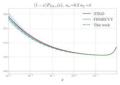
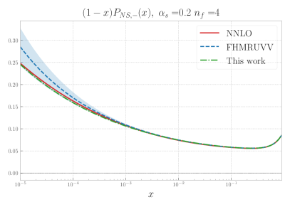
Figure 2.1: The aN³LO nonsinglet splitting functions $(1-x)P_{{\rm ns},+}(x,\alpha_{s})$ and $(1-x)P_{{\rm ns},-}(x,\alpha_{s})$, evaluated as a function of $x$ for $n_{f}=4$ and $\alpha_{s}=0.2$ in our approximation compared to the previous approximation of Ref. [22] (denoted FHMRUVV), for which the approximation uncertainty, as estimated by its authors, is also displayed. For comparison, the (exact) NNLO result is also shown.

2.4 aN³LO anomalous dimensions: singlet sector

In order to determine the singlet-sector anomalous dimension matrix entering Eq. (2.12), we must determine $\gamma_{{qq},{\rm ps}}$ that, together with the previously determined nonsinglet anomalous dimension, contributes to the $qq$ entry, Eq. (2.13), and then also the three remaining matrix elements $\gamma_{{qg}}$, $\gamma_{{gq}}$, and $\gamma_{{gg}}$.

For all matrix elements, the leading large-$n_{f}$ $\mathcal{O}(n_{f}^{3})$ contributions in Eq. (2.14) are known analytically [21], while for $\gamma_{{qq},{\rm ps}}$ [49] and $\gamma_{{gq}}$ [31] the $\mathcal{O}(n_{f}^{2})$ contributions are also known and we include all of them in $\gamma_{ij,n_{f}}^{(3)}(N)$.

Small-$x$ contributions in the singlet sector include, on top of the double-logarithmic contributions $a_{s}^{n+1}\ln^{2n-k}(x)$ that are present in the nonsinglet case, also single-logarithmic contributions $a_{s}^{n+1}\frac{1}{x}\ln^{n}(x)$. In Mellin space, this means that on top of order $2n-k+1$ subleading poles in $N=0$, there are also leading poles in $N=1$ of order $n-k+1$, i.e. $\frac{1}{(N-1)^{n-k+1}}$. The leading-power single logarithmic contributions can be extracted from the leading [50, 51, 52, 53, 54] and next-to-leading [55, 56, 57, 58, 59] high-energy resummation at LL$x$ [60] and NLL$x$ [61, 62, 63] accuracy. This allows for a determination of the coefficients of the leading $\frac{1}{(N-1)^{4}}$ and next-to-leading $\frac{1}{(N-1)^{3}}$ contributions to $\gamma^{(3)}_{gg}$ and of the next-to-leading $\frac{1}{(N-1)^{3}}$ contributions to $\gamma^{(3)}_{qg}$. The remaining entries can be obtained from these by using the color-charge (or Casimir scaling) relation $\gamma_{iq}=\frac{C_{F}}{C_{A}}\gamma_{ig}$ [64, 63]. Hence, we set

$$\gamma_{gg,\,N\to 1}^{(3)}(N) =c^{4}_{gg,\,N\to 1}\frac{1}{(N-1)^{4}}+c^{3}_{gg,\,N\to 1}\frac{1}{(N-1)^{3}};$$ (2.25)

$$\gamma_{qg,\,N\to 1}^{(3)}(N) =c^{3}_{qg,\,N\to 1}\frac{1}{(N-1)^{3}};$$ (2.26)

$$\gamma_{iq,\,N\to 1}^{(3)}(N) =\frac{C_{F}}{C_{A}}\gamma_{ig,\,N\to 1}^{(3)}(N),\quad i=q,\,g.$$ (2.27)

Although only the leading pole of $\gamma_{gq}$ satisfies Eq. (2.27) exactly, at NNLO this relation is only violated at the sub-percent level [65], so this is likely to be an adequate approximation also at this order: this approximation is also adopted in Ref. [30]. An important observation is that both NLO and NNLO coefficients of the leading poles, $\frac{1}{(N-1)^{2}}$ and $\frac{1}{(N-1)^{3}}$ respectively, vanish accidentally. Hence, at N³LO the leading poles contribute for the first time beyond leading order. The subleading poles can be determined up to NNLL accuracy [23] and, thus, fix the coefficients of the $\frac{1}{N^{7}}$, $\frac{1}{N^{6}}$ and $\frac{1}{N^{5}}$ subleading poles for all entries of the singlet anomalous dimension matrix. All these contributions are included in $\gamma_{ij,N\to 1}^{(3)}(N)$ and $\gamma_{ij,N\to 0}^{(3)}(N)$.

In the singlet sector, large-$x$ contributions whose Mellin transform is not suppressed in the large-$N$ limit only appear in the diagonal $qq$ and $gg$ channels. In the quark channel these are already included, through Eq. (2.13) in $\gamma_{{\rm ns},+,\,N\to\infty}^{(3)}(N)$, according to Eq. (2.24), while $\gamma^{(3)}_{qq,{\rm ps}}$ is suppressed in this limit. In the gluon-to-gluon channel they take the same form as in the nonsinglet and diagonal quark channel. Hence, we expand, as in Eq. (2.24),

$$\gamma_{gg,\,N\to\infty}^{(3)}(N)=A^{g}_{4}S_{1}(N)+B^{g}_{4}+C^{g}_{4}\frac{S_{1}(N)}{N}+D^{g}_{4}\frac{1}{N}\,.$$ (2.28)

The coefficients $A^{g}_{4}$, $B^{g}_{4}$, $C^{g}_{4}$ and $D^{g}_{4}$ are the counterparts of those of Eq. 2.24: the gluon cusp anomalous dimension was determined in Ref. [24] and the constant in Ref. [25], while the $C^{g}_{4}$ and $D^{g}_{4}$ coefficients can be determined using results from Refs. [66, 30].

Off-diagonal $qg$ and $qg$ splitting functions have logarithmically enhanced next-to-leading power behavior at large-$x$:

$$P_{ij}^{(3)}(x)=\sum_{k=0}^{6}\sum_{l=0}^{\infty}c^{k,l}_{ij,\,N\to\infty}(1-x)^{l}\ln^{k}(1-x).$$ (2.29)

For $l=0$ the coefficients of the higher logs $k=4,5,6$ can be determined from N³LO coefficient functions, based on a conjecture [27, 67] on the large-$x$ behavior of the physical evolution kernels that give the scale dependence of structure functions. The coefficient with the highest power $k=6$ cancels and thus we let

$$\gamma_{gq,\,N\to\infty}^{(3)}(N)=\sum_{k=4}^{5}c^{k,0}_{gq,\,N\to\infty} \mathcal{M}\left[\ln^{k}(1-x)\right](N),$$ (2.30)

$$\gamma_{qg,\,N\to\infty}^{(3)}(N)=\sum_{k=4}^{5}c^{k,0}_{qg,\,N\to\infty}\mathcal{M}\left[\ln^{k}(1-x)\right](N) +c^{k,1}_{qg,\,N\to\infty}\mathcal{M}\left[(1-x)\ln^{k}(1-x)\right](N),$$ (2.31)

where in $\gamma_{qg,\,N\to\infty}^{(3)}$ we have retained also the $l=1$ terms [29].

Finally, the pure singlet quark-to-quark splitting function starts at next-to-next-to-leading power as $x\to 1$, i.e. it behaves as $(1-x)\ln^{k}(1-x)$, with $k\leq 4$. The coefficients of the higher logs $k=3,4$ can be extracted by expanding the $x=1$ expressions from Refs. [27, 28]. Hence, we let

$$\gamma_{qq,{\rm ps},\,N\to\infty}^{(3)}(N)=\sum_{k=3}^{4}\left[c^{k,1}_{qq,{\rm ps},\,N\to\infty}\mathcal{M}\left[(1-x)\ln^{k}(1-x)\right](N)+c^{k,2}_{qq,{\rm ps},\,N\to\infty}\mathcal{M}\left[(1-x)^{2}\ln^{k}(1-x)\right](N)\right]$$ (2.33)

Note that for the $qq$ and $qg$ entries we also include the (known) next-to-leading power contributions, while we do not include them for $gq$ and $gg$ because for these anomalous dimension matrix elements a significantly larger number of higher Mellin moments is known, hence there is no risk that the inclusion of these contributions could contaminate the intermediate $x$ region where they are not necessarily dominant. The explicit expressions of $\gamma_{{\rm ns}\,\pm,\,N\to\infty}^{(3)}(N)$, $\gamma_{{\rm ns}\,\pm,\,N\to 0}^{(3)}(N)$ and $\gamma_{{\rm ns}\,\pm,\,N\to 1}^{(3)}(N)$ are all given in Appendix A.

As discussed in Sect. 2.1, the remainder contribution $\widetilde{\gamma}_{ij}^{(3)}(N)$, Eq. (2.16), is determined by expanding it over a set of basis functions and determining the expansion coefficients by demanding that the four components of the singlet anomalous dimension matrix reproduce the known moments. Specifically, these are the four moments computed in Ref. [26], the six additional moments for $\gamma_{qq,{\rm ps}}$ and $\gamma_{qg}$ computed in Ref. [28] and Ref. [29] respectively, and the additional moment $N=10$ for $\gamma_{gg}$ and $\gamma_{gq}$ evaluated in Ref. [30]. These constraints automatically implement momentum conservation:

$$\begin{split}\gamma_{qg}(N=2)+\gamma_{gg}(N=2)&=0\,,\\ \gamma_{qq}(N=2)+\gamma_{gq}(N=2)&=0\,.\end{split}$$ (2.34)

$\gamma_{gg}^{(3)}(N)$	$G^{gg}_{1}(N)$	$\mathcal{M}[(1-x)\ln^{3}(1-x)](N)$
	$G^{gg}_{2}(N)$	$\frac{1}{(N-1)^{2}}$
	$G^{gg}_{3}(N)$	$\frac{1}{N-1}$
	$\{H^{gg}_{1}(N),\ H^{gg}_{2}(N)\}$	$\frac{1}{N^{4}},\ \frac{1}{N^{3}},\ \frac{1}{N^{2}},\ \frac{1}{N+1},\ \frac{1}{N+2},\ \mathcal{M}[(1-x)\ln^{2}(1-x)](N),\ \mathcal{M}[(1-x)\ln(1-x)](N)$
$\gamma_{gq}^{(3)}(N)$	$G^{gq}_{1}(N)$	$\mathcal{M}[\ln^{3}(1-x)](N)$
	$G^{gg}_{2}(N)$	$\frac{1}{(N-1)^{2}}$
	$G^{gq}_{3}(N)$	$\frac{1}{N-1}$
	$\{H^{gq}_{1}(N),\ H^{gq}_{2}(N)\}$	$\frac{1}{N^{4}},\ \frac{1}{N^{3}},\ \frac{1}{N^{2}},\ \frac{1}{N+1},\ \frac{1}{N+2},\ \mathcal{M}[\ln^{2}(1-x)](N),\ \mathcal{M}[\ln(1-x)](N)$
$\gamma_{qg}^{(3)}(N)$	$G^{qg}_{1}(N)$	$\mathcal{M}[\ln^{3}(1-x)](N)$
	$G^{qg}_{2}(N)$	$\frac{1}{(N-1)^{2}}$
	$G^{qg}_{3}(N)$	$\frac{1}{N-1}-\frac{1}{N}$
	$G^{qg}_{4,\dots,8}(N)$	$\frac{1}{N^{4}},\ \frac{1}{N^{3}},\ \frac{1}{N^{2}},\ \frac{1}{N},\ \mathcal{M}[\ln^{2}(1-x)](N)$
	$\{H^{qg}_{1}(N),\ H^{qg}_{2}(N)\}$	$\mathcal{M}[\ln(x)\ln(1-x)](N),\ \mathcal{M}[\ln(1-x)](N),\ \mathcal{M}[(1-x)\ln^{3}(1-x)](N)$
		$\mathcal{M}[(1-x)\ln^{2}(1-x)](N),\ \mathcal{M}[(1-x)\ln(1-x)](N),\ \frac{1}{1+N}$
$\gamma_{qq,{\rm ps}}^{(3)}(N)$	$G^{qq,{\rm ps}}_{1}(N)$	$\mathcal{M}[(1-x)\ln^{2}(1-x)](N)$
	$G^{qq,{\rm ps}}_{2}(N)$	$-\frac{1}{(N-1)^{2}}+\frac{1}{N^{2}}$
	$G^{qq,{\rm ps}}_{3}(N)$	$-\frac{1}{(N-1)}+\frac{1}{N}$
	$G^{qq,{\rm ps}}_{4,\dots,8}(N)$	$\frac{1}{N^{4}},\ \frac{1}{N^{3}},\ \mathcal{M}[(1-x)\ln(1-x)](N)$
		$\mathcal{M}[(1-x)^{2}\ln(1-x)^{2}](N),\ \mathcal{M}[(1-x)\ln(x)](N)$
	$\{H^{qq,{\rm ps}}_{1}(N),\ H^{qq,{\rm ps}}_{2}(N)\}$	$\mathcal{M}[(1-x)(1+2x)](N),\ \mathcal{M}[(1-x)x^{2}](N)$,
		$\mathcal{M}[(1-x)x(1+x)](N),\ \mathcal{M}[(1-x)](N)$

Table 2.2: The set of basis functions $G^{ij}_{\ell}(N)$ and $H^{ij}_{\ell}(N)$ used to parametrize the singlet sector remainder anomalous dimensions matrix elements $\widetilde{\gamma}_{ij}^{(3)}(N)$ according to Eq. (2.16).

The set of basis functions is chosen based on the idea of constructing an approximation that reproduces the singularity structure of the Mellin transform of the anomalous dimension viewed as analytic functions in $N$ space [48], hence corresponding to the leading and subleading (i.e. rightmost) $N$-space poles with unknown coefficients as well as the leading unknown large-$N$ behavior. Specifically, the functions $G^{ij}$ are chosen as follows.

1. The function $G^{ij}_{1}(N)$ reproduces the leading unknown contribution in the large-$N$ limit, i.e. the unknown term in Eq. (2.29) with highest $k$ and lowest $l$.

2. The functions $G^{ij}_{2}(N)$ and $G^{ij}_{3}(N)$ reproduce the first two leading unknown contributions in the small-$N$ limit, i.e. the unknown $\frac{1}{(N-1)^{k}}$ leading poles with highest and next-to-highest values of $k$, i.e. $k=2$ and $k=1$. For $\gamma_{qq,{\rm ps}}$ and $\gamma_{qg}$ a subleading small-$x$ pole with the same power and opposite sign is added to the leading pole with respectively $k=1,\,2$ and $k=1$, so as to leave unaffected the respective large-$x$ leading power behavior Eqs. (2.31-2.33).

3. For $\gamma_{qq,{\rm ps}}$ and $\gamma_{qg}$, for which an additional five moments are known, the functions $G^{qj}_{4,\dots,8}(N)$ reproduce subleading small- and large-$N$ terms.

The functions $H^{ij}$ are chosen as follows.

1. The functions $H^{gj}_{1}(N),H^{gj}_{2}(N)$ in the gluon sector, where only five moments are known exactly, are chosen to reproduce subleading small- and large-$N$ terms, i.e. similar to $G^{qj}_{4,\dots,8}(N)$.

2. The functions $H^{qg}_{1}(N),H^{qg}_{2}(N)$ are chosen as subleading and next-to-leading power large-$x$ terms and the remaining unknown leading small-$N$ pole.

3. The functions $H^{qq,\,{\rm ps}}_{1}(N),H^{qq,\,{\rm ps}}_{2}(N)$ are chosen as low-order polynomials, i.e., sub-subleading small-$x$ poles.

The number of basis functions is greater for anomalous dimension matrix elements for which less exact information is available: 7 in the gluon sector (i.e. $gg$ and $gq$), 6 for the $qg$ entry and 4 for the pure singlet entry. For the $gg$ entry two combinations are discarded as they lead to unstable (oscillating) results and we thus end up with $\widetilde{N}_{gg}=19$, $\widetilde{N}_{gq}=21$, $\widetilde{N}_{qg}=15$, and $\widetilde{N}_{qq}=6$ different parametrizations. The full set of basis functions $G^{ij}$ and $H^{ij}$ is listed in Table 2.2.

Upon combining the exactly known contributions with the $\widetilde{N}_{ij}$ remainder terms according to Eq. (2.15) we end up with an ensemble of $\widetilde{N}_{ij}$ instances of $\gamma_{ij}^{(3),\,(k)}(N)$ for each singlet anomalous dimension matrix element and the final matrix elements $\gamma_{ij}^{(3)}(N)$ and their uncertainties $\sigma_{ij}(N)$ are computed using Eqs. (2.17) and (2.21) respectively.

2.5 Results: aN³LO splitting functions

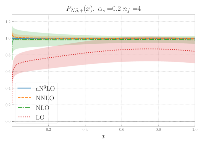
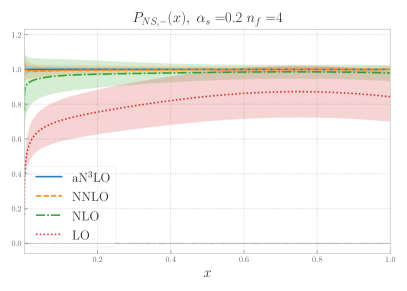
Figure 2.2: The nonsinglet splitting functions at LO, NLO, NNLO, and aN³LO, normalized to the aN³LO central value and with a linear scale on the $x$ axis. In each case we shown also the uncertainty due to missing higher orders (MHOU) estimated by scale variation according to Refs. [35, 36].

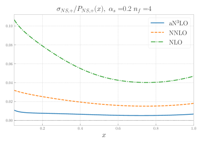
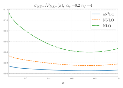
Figure 2.3: The relative size of the uncertainty due to missing higher orders (MHOU) on the splitting functions of Fig. 2.2.

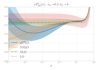
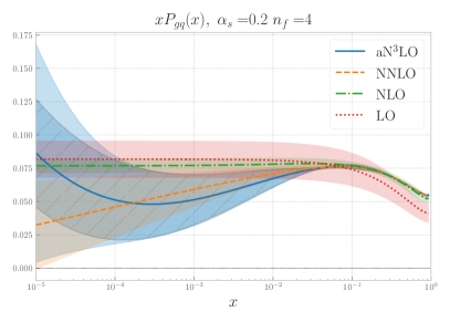
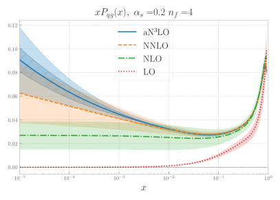
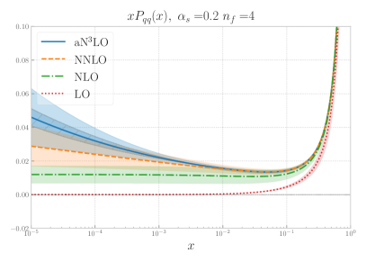
Figure 2.4: The singlet matrix of splitting functions $xP_{ij}$ at LO, NLO, NNLO and aN³LO. From left to right and from top to bottom the $gg$, $gq$, $qg$ and $qq$ entries are shown. The MHOU estimated by scale variation is shown to all orders. At aN³LO the dark blue band corresponds to IHOU only, while the light blue band is the sum in quadrature of IHOU and MHOU.

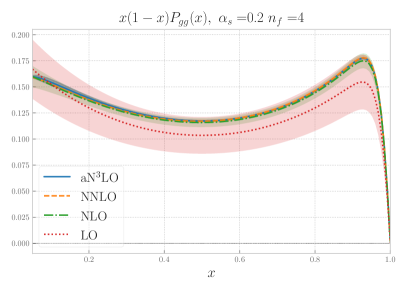
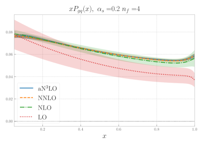
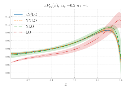
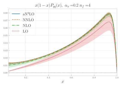
Figure 2.5: Same as Fig. 2.4 with a linear scale on the $x$ axis, and plotting $(1-x)xP_{ii}$ for diagonal entries.

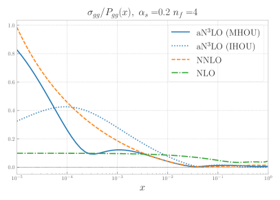
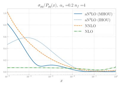
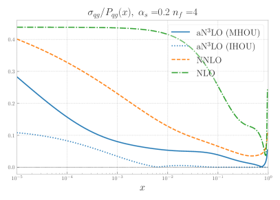
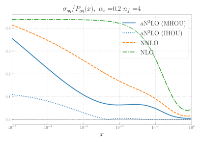
Figure 2.6: Same as Fig. 2.3 for the singlet splitting function matrix elements. At NLO and NNLO we show the MHOU, while at aN³LO we also show the IHOU.

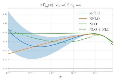
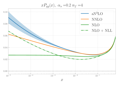
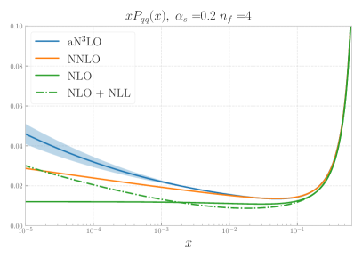
Figure 2.7: Comparison of the NLO, NNLO, and aN³LO splitting functions (same as in Fig. 2.4) to the small-$x$ resummed NLO+NLL result of Ref. [68]. Only the IHOU on the aN³LO result is shown.

We now present the aN³LO splitting functions constructed following the procedure described in Sects. 2.1–2.4. The nonsinglet result, already compared in Fig. 2.1 to the previous approximation of Ref. [22], is shown in Fig. 2.2 at the first four perturbative orders as a ratio to the aN³LO result. For each order we include the MHOU determined by scale variation according to Refs. [35, 36] and recall that there are no IHOU in the nonsinglet sector. As the nonsinglet splitting function are subdominant at small $x$ we only show the plot with a linear scale in $x$. The relative size of the MHOU is shown in Fig. 2.3.

Inspecting Figs. 2.2 and 2.3 reveals good perturbative convergence for all values of $x$. Specifically, the differences between two subsequent perturbative orders are reduced as the accuracy of the calculation increases, and, correspondingly, the MHOUs associated to factorization scale variations decrease with the perturbative accuracy. Indeed, the MHOU appears to reproduce well the observed behaviour of the higher orders, with overlapping uncertainty bands between subsequent orders except at LO at the smallest $x$ values.

Based on these results it is clear that in the nonsinglet sector the N³LO contribution to the splitting function is essentially negligible except at the smallest $x$ values, as shown in Fig. 2.1. Consequently, for all practical purposes we can consider the current approximation to the nonsinglet anomalous dimension to be essentially exact, and with negligible MHOU.

The situation in the singlet sector is more challenging. The singlet matrix of splitting functions is shown in Figs. 2.4 and 2.5, respectively with a logarithmic or linear scale on the $x$ axis. Because the diagonal splitting functions are distributions at $x=1$ in the linear scale plots we display $x(1-x)P_{ii}$. The corresponding relative size of the MHOU is shown in Fig. 2.6 for the first four perturbative orders, along with the IHOU on the aN³LO result, determined using Eq. (2.21).

A different behaviour is observed for the quark sector $P_{qi}$ and for the gluon sector $P_{gi}$. In the quark sector, the MHOU decreases with perturbative order for all $x$, but it remains sizable at aN³LO for essentially all $x$, of order 5% for $10^{-2}\lesssim x\lesssim 10^{-1}$. In the gluon sector instead for $x\gtrsim 0.03$ the MHOU is negligible, but at smaller $x$ it grows rapidly, and in fact at very small $x$ it becomes larger than the NLO MHOU. This is due to the presence of leading small-$x$ logarithms, Eq. (2.25), which are absent at NLO. In fact the true gluon-sector MHOU at very small $x$ is likely to be underestimated by scale variation, because while it generates the fourth-order leading pole present in the N⁴LO (the fifth-order pole vanishes), it fails to generate the sixth-order pole known to be present in the N⁵LO splitting function.

We now turn to the IHOU and find again contrasting behaviour in the different sectors. In the quark sector, thanks to the large number of known Mellin moments and the copious information on the large-$x$ limit, the IHOU are significantly smaller than the MHOU, by about a factor three, and become negligible for $x\gtrsim 10^{-2}$. In the gluon sector instead the IHOU, while still essentially negligible for $x\gtrsim 0.1$, is larger than the MHOU except at very small $x\lesssim 10^{-4}$ where the MHOU dominates.

Consequently, for all matrix elements at large $x\gtrsim 0.1$ the behaviour of the singlet is similar to the behaviour of the nonsinglet: IHOU and MHOU are both negligible, meaning that aN³LO results are essentially exact, and the perturbative expansion has essentially converged, see Fig. 2.5. At smaller $x$, while the aN³LO and NNLO results agree within uncertainties, the uncertainties on the aN³LO are sizable, dominated by MHOUs in the quark channel and by IHOUs in the gluon channel.

In the singlet sector the most dramatic impact of the aN³LO correction is at small $x$. It is thus interesting to compare the aN³LO singlet splitting functions with those obtained by the resummation of leading and next-to-leading order small-$x$ logarithms of Ref. [68], namely the two highest powers of $\ln x$ contained in the N³LO result; this comparison is shown in Fig. 2.7. The agreement of all four entries $xP_{gg}$, $xP_{gq}$, $xP_{qg}$ and $xP_{qq}$ is remarkably good and well within the uncertainties in the two approaches. In particular the dip in $xP_{gg}$ at intermediate $x$ at aN³LO (albeit with significant IHOU) is also a feature of the resummation. This is nontrivial, as the resummation includes only the asymptotic LL$x$ and NLL$x$ singularities at $N=1$, but none of the subleading results incorporated at aN³LO. Instead, it uses a symmetrization which resums collinear and anti-collinear logarithms in the small-$x$ expansion, and the effects of running coupling which change the nature of the small-$x$ singularity (from a fourth order pole at $N=1$ in the fixed order N³LO result to a simple pole a little further to the right on the real axis).

That both the resummed and fixed order approaches converge to very similar results, at least in the range of $x$ relevant for HERA and LHC, is very reassuring. It shows that in a global fit with current data, while NLL$x$ resummation significantly improves the quality of a fixed order NNLO fit [69], the same improvement should also be seen by adding aN³LO corrections. Thus to find evidence for small-$x$ resummation at aN³LO, it will probably be necessary to go to yet smaller values of $x$, e.g. below $10^{-5}$, where the fixed order and resummed results will eventually diverge again.

2.6 Results: aN³LO evolution

The aN³LO anomalous dimensions discussed in the previous sections have been implemented in the Mellin-space open-source evolution code EKO [40] which enters the new pipeline [70] adopted by NNPDF in order to produce theory predictions used for PDF determination. The parametrization is expressed in terms of a basis of Mellin space functions which are numerically efficient to evaluate. In order to achieve full aN³LO accuracy, in addition to the anomalous dimensions, the four-loop running of the strong coupling constant $\alpha_{s}(Q)$ and the N³LO matching conditions dictating the transitions between schemes with different numbers of active quark flavor have also been implemented.

The N³LO matching conditions have been presented in Ref. [71] and subsequently computed analytically in Refs. [72, 73, 74, 75, 76, 77, 78, 79, 80, 81]. The exception is the $a_{Hg}^{(3)}$ entry of the matching condition matrix, which is still unknown and which instead is parametrized using the first 5 known moments [71] and the LL$x$ contribution as done in Ref. [83]. Also these matching conditions are implemented in EKO and thus it is possible to assess the impact of the inclusion of aN³LO terms on perturbative evolution.

In Fig. 2.8 we compare the result of evolving a fixed set of PDFs from $Q_{0}=1.65$ GeV up to $Q=100$ GeV at NLO, NNLO, and aN³LO. We take as input the NNPDF4.0NNLO PDF set, and show results normalized to the aN³LO evolution. Results are shown for all the combinations that evolve differently, as discussed in Sect. 2.1, namely the singlet, gluon, total valence and nonsinglet $\pm$ combinations, with a logarithmic scale on the $x$ axis for the singlet sector and a linear scale for the valence and nonsinglet combinations.

In all cases the perturbative expansion appears to have converged everywhere, with almost no difference between NNLO and aN³LO except at small $x\lesssim 10^{-3}$, where singlet evolution is weaker at aN³LO than at NNLO due to the characteristic dip seen in the gluon sector splitting functions of Fig. 2.4. Because the gluon-driven small-$x$ rise dominates small-$x$ evolution this is a generic feature of all quark and gluon PDFs in this small-$x$ region. It is interesting to observe that this is an all-order feature that persists upon small-$x$ resummation, as already discussed at the end of Sect. 2.5 and seen in Fig. 2.7. In fact, the total theory uncertainty at aN³LO is at the sub-precent level for all $x\gtrsim 10^{-3}$. Hence, not only has the MHOU become negligible, but also the effect of IHOU on PDF evolution is only significant at small $x$.

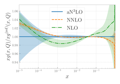
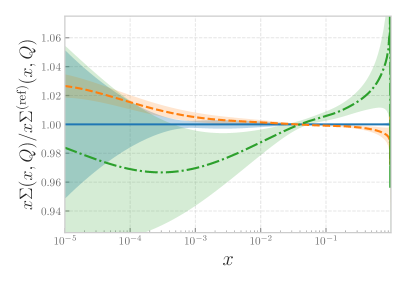
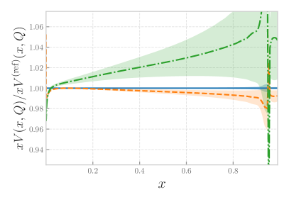
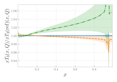
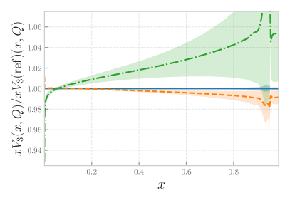
Figure 2.8: Comparison of the result obtained evolving from $Q_{0}=1.65$ GeV to $Q=100$ GeV at NLO, NNLO, and aN³LO using NNPDF4.0 NNLO as fixed starting PDF. Results are shown as ratio to the aN³LO (from left to right and from top to bottom) for the gluon and singlet $\Sigma$, and for the $V$, $V_{3}$ and $T_{3}$ quark eigenstates of perturbative evolution (see Sect. 2.1). The total theory uncertainty is shown in all cases, i.e. the MHOU at NLO and NNLO, and the sum in quadrature of MHOU and IHOU at aN³LO.

2.7 Comparison to other groups

We finally compare our approximation of the N³LO splitting functions to other recent results from Refs. [32, 28, 29, 30]. While the approach of Refs. [28, 29, 30] (FHMRUVV, henceforth) is very similar to our own, with differences only due to details of the choice of basis functions, a rather different approach is adopted in Ref. [32] (MSHT20, henceforth). There, the approximation is constructed from similar theoretical constraints (small-$x$, large-$x$ coefficients and Mellin moments), but supplementing the parametrization with additional nuisance parameters, which control the uncertainties arising from unknown N³LO terms. However, these approximations are taken as a prior, and the nuisance parameters are fitted to the data along with the PDF parameters. The best-fit values of the parameters determine the posterior for the splitting function, and their uncertainties are interpreted as the final IHOU on it. A consequence of this procedure is that the posterior can reabsorb not only N³LO corrections, but any other missing contribution, of theoretical or experimental origin.

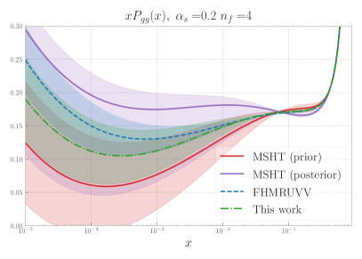
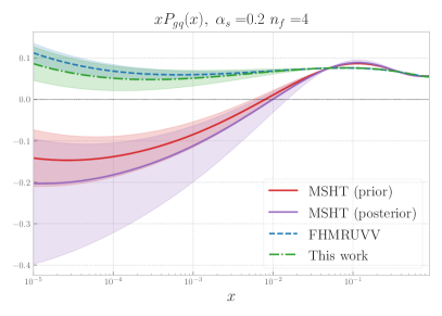
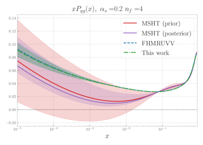
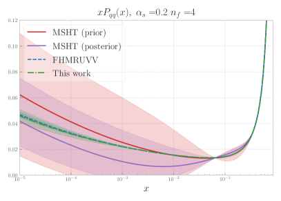
Figure 2.9: Same as Fig. 2.4, now comparing our aN³LO result to those of Ref. [32] (MSHT20) and Refs. [28, 29, 30] (FHMRUVV). In all cases the uncertainty band correspond to the IHOU as estimated by the various groups. For the MSHT20 results, we display both the prior and the posterior parametrizations (see text).

The comparison is presented in Fig. 2.9, for all the four singlet splitting functions. For the MSHT20 results both prior and posterior are displayed. As expected, excellent agreement is found with the FHMRUVV result, for all splitting functions and for all $x$, especially for the $P_{qg}$ and $P_{qq}$ splitting functions, for which the highest number of Mellin moments is known. Good qualitative agreement is also found for $P_{gq}$ and $P_{gg}$, although at small $x$ IHOUs are larger and consequently central values differ somewhat more, though still in agreement within uncertainties. Coming now to MSHT20 results, good agreement is found with the prior, except for $P_{gq}$, for which MSHT20 shows a small-$x$ dip accompanied by a large-$x$ bump. The different small-$x$ behaviour is likely due to the fact that MSHT20 do not enforce the color-charge relation Eq. (2.27) at NLL$x$, with the large-$x$ bump then following from the constraints Eq. (2.34). Also, in the quark sector the MSHT20 prior has significantly larger IHOUs due to the fact that it does not include the more recent information on Mellin moments from Refs. [23, 28, 29, 30, 31], which were not available at the time of the MSHT20 analysis [32]. At the level of posterior, however, significant differences appear also for $P_{gg}$, while persisting for $P_{gq}$. This means that the gluon evolution at aN³LO is being significantly modified by the data entering the global fit, and it is not fully determined by the perturbative computation. Further benchmarks of aN³LO splitting functions will be presented in Ref. [84].

3 N³LO partonic cross-sections

A PDF determination at N³LO requires, in addition to the splitting functions discussed in Sect. 2, hard cross sections at the same perturbative order. Exact N³LO massless DIS coefficient functions have been known for several years [1, 2, 3, 4, 85, 86], while massive coefficient functions are only available in various approximations [83, 87, 88]. For hadronic processes, N³LO results are available for inclusive Drell-Yan production for the total cross-section [12, 11, 8] as well as for rapidity [18] and transverse momentum distributions [19], though neither of these is publicly available.

We now describe the implementation of these corrections. First, we review available results on DIS coefficient functions and summarize the main features of the approximation that we will use for massive coefficient functions [88, 87]. Next we discuss how massless and massive DIS coefficient functions are combined to extend the FONLL general-mass variable-flavor number scheme to $\mathcal{O}\left(\alpha_{s}^{3}\right)$. Finally, we discuss N³LO corrections for hadronic processes and different options for their inclusion in PDF determination.

3.1 N³LO corrections to DIS structure functions

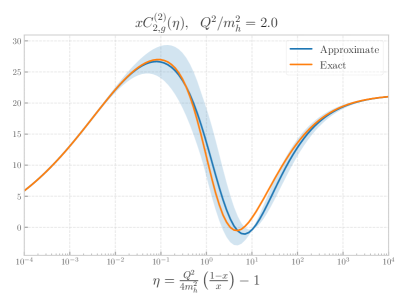
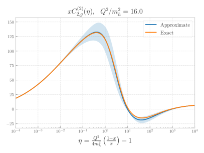
Figure 3.1: Comparison of the exact NNLO massive gluon-initiated coefficient function $xC_{2,g}^{(2)}(\eta)$ to the approximation Eq. (3.3) from Ref. [87], plotted as a function of $\eta$, Eq. (3.5), for fixed $Q^{2}$. Results are shown for two different values of $Q^{2}$, one close to threshold $Q^{2}=2m_{h}^{2}$ (left) and one at high scales $Q^{2}=16m_{h}^{2}$ (right). The uncertainty on the approximate result is obtained by varying the interpolating functions $f_{1}(x)$ and $f_{2}(x)$ in Eq. (3.3).

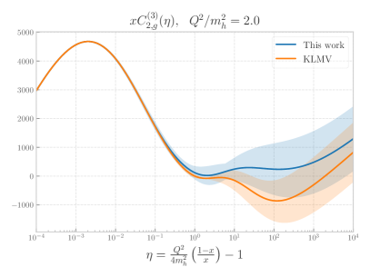
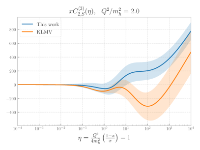
Figure 3.2: The approximate N³LO massive gluon (left) and quark singlet (right) coefficient functions as a function of $\eta$ for fixed $Q^{2}=2m_{h}^{2}$. Our result based on the approximation of Ref. [87] is compared to the approximation of Ref. [83] (KLMV).

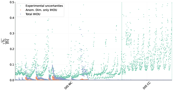
Figure 3.3: Square root of the diagonal entries of the IHOU covariance matrix for the DIS datasets normalized to the experimental central value $D_{i}$. We show the IHOU before and after adding to the covariance matrix Eq. (2.20) that accounts for uncertainty on anomalous dimensions the extra component Eq. (3.6) due to the massive coefficient function. The experimental uncertainty is also shown for comparison.

The DIS structure functions $F_{i}$ are evaluated from the convolution of PDFs and coefficient functions

$$\begin{split}F_{i}(x,Q^{2})=\sum_{k=1}^{n_{f}}C_{i,k}(x,\alpha_{s})\otimes xq^{+}_{k}(x,Q^{2})&+C_{i,g}(x,\alpha_{s})\otimes xg(x,Q^{2})\,,\qquad i=\{2,L\}\,,\\ xF_{3}(x,Q^{2})=\sum_{k=1}^{n_{f}}C_{3,k}(x,\alpha_{s})&\otimes xq^{-}_{k}(x,Q^{2})\,,\end{split}$$ (3.1)

with the coefficient functions evaluated in a perturbative QCD expansion

$$C_{i,k}(x,\alpha_{s}(Q^{2}))=\sum_{n=0}\alpha_{s}^{n}(Q^{2})C_{i,k}^{(n)}(x)\,.$$ (3.2)

Coefficient functions with all quarks assumed to be massless were evaluated at N³LO in [1, 2] for neutral-current charged-lepton scattering and recently independently benchmarked in [86]. The corresponding results for charged-current scattering were presented in [3, 4, 85].

For sufficiently low scale, some or all of the heavy quark masses cannot be neglected. Heavy quark contributions to structure functions may be treated in a decoupling scheme [89], in which heavy quarks do not contribute to the running of $\alpha_{s}$ and to PDF evolution, and coefficient functions acquire a dependence on the heavy quark mass $m_{h}$ [90]: $C_{i,k}=C_{i,k}(x,\alpha_{s},m^{2}_{h}/Q^{2})$ (massive coefficient functions, henceforth). The massive coefficient functions are known exactly up to NNLO for photon [91, 92], Z [93, 94] and W [95] exchange (for massless to massive transitions only) while at N³LO only partial results are available [96, 97, 83, 88] or in the $Q^{2}\gg m_{h}^{2}$ limit [72, 71, 74, 75, 98, 77].

We adopt an approximation for the N³LO contribution $C_{i,k}^{(3)}(x,\alpha_{s},m^{2}_{h}/Q^{2})$ to massive coefficient functions for photon-induced DIS and neglect the axial-vector coupling of the Z boson, while we treat heavy quarks in the massless approximation for the W boson exchange. Such an approximation, based on known partial results, has been presented in Ref. [83], and recently revisited in Ref. [87]. The approaches of these references rely on the same known exact results, and differ in the details of the way they are combined and interpolated. Here we will follow Ref. [87], see also Ref. [88], to which we refer for further details. Exact results come from threshold resummation and high-energy resummation, and are further combined with the asymptotic large-$Q^{2}$ limit, thereby ensuring that the approximate massive coefficient function reproduces the exact massless result in the $Q^{2}/m_{h}^{2}\to\infty$ limit. In the approach of Refs. [87, 88] the massive coefficient functions are written as

$$C_{i,k}^{(3)}(x,m_{h}^{2}/Q^{2})=C_{i,k}^{(3),{\rm thr}}(x,m_{h}^{2}/Q^{2})f_{1}(x)+C_{i,k}^{(3),{\rm asy}}(x,m_{h}^{2}/Q^{2})f_{2}(x)\,,$$ (3.3)

where $C_{i,k}^{(3),{\rm thr}}$ and $C_{i,k}^{(3),{\rm asy}}$ correspond to the contributions coming from differently resummations, and $f_{1}(x)$ and $f_{2}(x)$ are two suitable matching functions.

For massive quarks the threshold limit is $x\to x_{\rm max}$ with $x_{\rm max}=\frac{Q^{2}}{4m_{h}^{2}+Q^{2}}$ or $\beta\to 0$, with $\beta\equiv\sqrt{1-\frac{4m_{h}^{2}}{s}}$ and $s=Q^{2}\frac{1-x}{x}$ the centre-of-mass energy of the partonic cross-section. In this limit, the coefficient function contains logarithmically enhanced terms of the form $\alpha_{s}^{n}\ln^{m}\beta$ with $m\leq 2n$ due to soft gluon emission, which are predicted by threshold resummation [99]. Further contributions of the form $\alpha_{s}^{n}\beta^{-m}\ln^{l}\beta$, with $m\leq n$, arise from Coulomb exchange between the heavy quark and antiquark, and can also be resummed using non-relativistic QCD methods [100]. At N³LO all these contributions are known and can be extracted from available resummed results [83]; they are included in $C_{i,k}^{(3),{\rm thr}}$.

In the high-energy limit, the coefficient function contains logarithmically enhanced terms of the form $\alpha_{s}^{n}\ln^{m}x$ with $m\leq n-2$, which are determined at all orders through small-$x$ resummation at the LL level [97], from which the N³LO expansion can be extracted [83]. This result can be further improved [87, 88] by including a particular class of NLL terms related to NLL perturbative evolution and the running of the coupling. In the approach of Refs. [87, 88] the high-energy contributions are combined into $C_{i,k}^{(3),{\rm asy}}$ with the asymptotic $Q^{2}\gg m_{h}^{2}$ limit of the coefficient function in the decoupling scheme [72, 71, 74, 75, 98, 77], while subtracting overlap terms. This ensures that in the $Q^{2}\gg m_{h}^{2}$ limit, the structure function, computed from $C_{i,k}^{(3),{\rm asy}}$ combined with decoupling-scheme PDFs, coincides with the structure function computed in the limit in which the heavy quark mass is neglected and the heavy quark is treated as a massless parton. However, the asymptotic limit can only be determined approximately since in particular some of the matching conditions are not fully known.

The interpolating functions, used to combine the two contributions in Eq. (3.3), are chosen to satisfy the requirements

$$\begin{split}f_{1}(x)\xrightarrow[x\to 0]{}0,&\quad f_{1}(x)\xrightarrow[x\to x_{\rm max}]{}1\,,\\ f_{2}(x)\xrightarrow[x\to 0]{}1,&\quad f_{1}(x)\xrightarrow[x\to x_{\rm max}]{}0\,,\end{split}$$ (3.4)

which ensure that the threshold contribution vanishes in the small-$x$ limit and conversely. This guarantees that the approximation Eq. (3.3) is reliable in a broad kinematic range in the $(x,Q^{2})$ plane: $C_{i,k}^{(3),{\rm asy}}$ reproduces the massless limit for large $Q^{2}$ values and for all values of $x$, including the small-$x$ limit, while $C_{i,k}^{(3),{\rm thr}}$ describes the threshold limit, with $x$ close to $x_{\rm max}$. An uncertainty on the approximate coefficient function can be constructed varying the functional form of the interpolating functions, as well as that of terms which are not fully known. This includes the NLL small-$x$ resummation, the matching functions that enter the asymptotic high $Q^{2}$ limit and constant (i.e. $\beta$-independent) terms in the threshold limit. This uncertainty vanishes in the $x\to x_{\rm max}$ limit, for which the exact known limit is reproduced, and becomes larger in the intermediate $\eta$ region. We refer to Ref. [87] for a detailed discussion of the construction of this uncertainty.

As a validation of this approximation, in Fig. 3.1 we compare a NNLO approximation constructed using the same methodology to the exact result for the massive gluon-initiated coefficient function $xC_{2,g}^{(2)}(\eta)$, expressed in terms of the variable

$$\eta=\frac{Q^{2}(1-x)}{4m_{h}^{2}x}-1\,.$$ (3.5)

Results are shown for two different values of the $Q^{2}/m_{h}^{2}$ ratio, close to threshold and at higher scales. Note that $\eta\to 0$ corresponds to $x\to x_{\rm max}$ (threshold limit), while $\eta\to\infty$ corresponds to either $Q^{2}/m_{h}^{2}\to\infty$ for fixed $x$ (asymptotic limit), or $x\to 0$ for fixed $Q^{2}$ (high-energy limit). In this case the uncertainty band is obtained by varying the interpolating functions only.

The results found using the same procedure for the gluon and quark singlet coefficient functions at N³LO are displayed in Fig. 3.2, compared to the approximation of Ref. [83], each shown with the respective uncertainty estimate. Good agreement between the different approximations is found, especially for the dominant gluon coefficient function. The approximations agree in the asymptotic $\eta\to 0$ and $\eta\to\infty$ limits, but differ somewhat at intermediate $\eta$.

The uncertainty involved in the approximation can be included as a further IHOU, alongside that discussed in Sect. 2.2, through an additional contribution to the theory covariance matrix. Namely, we define

$$\text{cov}^{C}_{mn}=\frac{1}{2}\left(\Delta_{m}(+)\Delta_{n}(+)+\Delta_{m}(-)\Delta_{n}(-)\right).$$ (3.6)

Here $\Delta_{m}(\pm)$ is the shift in the prediction for the $m$-th DIS data point obtained by replacing the central approximation to the massive coefficient function with the upper or lower edge of the uncertainty range determined in Ref. [87] and shown as an uncertainty band in Fig. 3.2. Note that unlike in Eq. (2.20), we divide by the number of independent variations, without decreasing it by one, because the central value is not the average of the variations, and thus is independent. The contribution Eq. (3.6) is then added to the IHOU covariance matrix as a further term on the right-hand side of Eq. (2.20).

The impact of this contribution to the IHOU is assessed in Fig. 3.3, where the square root of the diagonal component of the covariance matrix is shown for all the DIS data points in our dataset, comparing the IHOU before and after adding to Eq. (2.20) the extra component Eq. (3.6) due to the IHOU on the massive coefficient function. It is clear that the impact of IHOUs due to perturbative evolution is generally negligible, in agreement with the results discussed in Sect. 2.6 and shown in Fig. 2.8: IHOUs on splitting functions are only significant at small $x$, but available small-$x$ data are at relatively low scale where the evolution length is small. The impact of IHOUs on massive coefficient functions is relevant for data on tagged bottom and charm structure functions, but otherwise moderate and only significant for structure function data close to the heavy quark production thresholds.

3.2 A general-mass variable flavor number scheme at N³LO

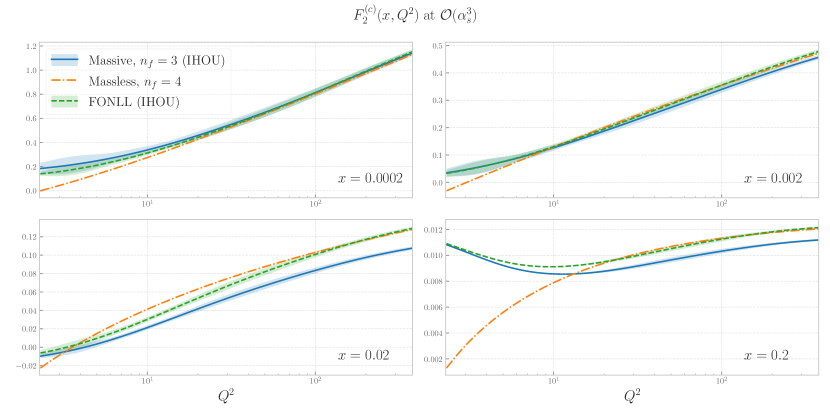
Figure 3.4: The charm structure function $F^{(c)}_{2}(x,Q^{2},m_{c}^{2})$ in the FONLL-E scheme, compared to the massive and massless scheme results (see text). Results are shown as a function of $Q^{2}$ for $x=2\times 10^{-4}$ (top left), $x=2\times 10^{-3}$ (top right), $x=2\times 10^{-2}$ (bottom left), and $x=2\times 10^{-1}$ (bottom right). The uncertainty shown on the FONLL and massive curves is the IHOU on the heavy quark coefficient functions Eq. (3.6).

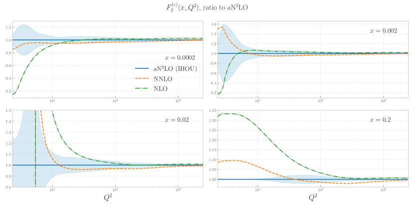
Figure 3.5: Same as Fig. 3.4, now comparing the FONLL-A (used at NLO $\mathcal{O}\left(\alpha_{s}\right)$), FONLL-C (used at NNLO $\mathcal{O}\left(\alpha_{s}^{2}\right)$), and FONLL-E (used at N³LO $\mathcal{O}\left(\alpha_{s}^{3}\right)$), all shown as a ratio to FONLL-E. The FONLL-E result includes the IHOU on the heavy quark coefficient functions Eq. (3.6).

The N³LO DIS coefficients functions described in the previous section enable the extension to $\mathcal{O}\left(\alpha_{s}^{3}\right)$ of the FONLL [101] general-mass variable flavor number scheme for DIS [42, 43, 44]. The goal of the FONLL strategy is results that are accurate and reliable for all values of $Q^{2}$ from the production threshold $Q^{2}\sim m_{h}^{2}$ to the asymptotic limit $Q^{2}\gg m_{h}^{2}$.

Assuming a single heavy quark, calculations performed in a decoupling scheme with $n_{\ell}$ light quarks retain the full dependence on the heavy quark mass and include the contribution of heavy quarks at a fixed perturbative order (massive scheme, henceforth). Calculations performed in a scheme in which the heavy quark is treated as massless (massless scheme, henceforth), and endowed with a PDF that satisfies perturbative matching conditions, resums logarithms of $Q^{2}/m_{h}^{2}$ to all orders through the running of the coupling and the evolution of PDFs, but does not include terms that are suppressed as powers of $\frac{m_{h}^{2}}{Q^{2}}$ and thus become relevant when $Q^{2}\mathrel{\hbox to0.0pt{\lower 4.0pt\hbox{\hskip 1.0pt$\sim$}\hss}\raise 1.0pt\hbox{$>$}}m_{h}^{2}$. The FONLL prescription matches the two calculations by defining

$$F^{{\rm FONLL}}_{i}=F_{i}^{(n)}(x,Q^{2},m_{h}^{2})+F_{i}^{(n+1)}(x,Q)-F_{i}^{(n,0)}(x,\ln(Q^{2}/m_{h}^{2}))\,,\qquad\ i={2,L,3}\,,$$ (3.7)

where $F_{i}^{(n)}$ denotes the massive computation in which the $(n+1)$-th (heavy) flavor decouples, $F_{i}^{(n+1)}$ the one in which it is treated as massless, and $F_{i}^{(n,0)}$ is the asymptotic large-$Q^{2}$ limit of the massive scheme calculation, which depends only logarithmically on the heavy quark mass. This construction reduces to the decoupling calculation for $Q^{2}\approx m_{h}^{2}$ and to the massless one for $Q^{2}\gg m_{h}^{2}$.

The FONLL prescription of Eq. (3.7) was implemented in Ref. [42, 43, 44] for DIS to NNLO, by expressing all terms on the right-hand side in terms of $\alpha_{s}$ and PDFs all defined in the massless scheme. This has the advantage of providing an expression that can used with externally provided PDFs, that are typically available only in a single factorization scheme for each value of the scale $Q$.

However, the recent EKO code [40] allows, at any given scale, the coexistence of PDFs defined in schemes with a different number of massless flavors. Furthermore, the recent YADISM program [41] implements DIS coefficient functions corresponding to all three contributions on the right-hand side of Eq. (3.7). It is then possible to implement the FONLL prescription Eq. (3.7) by simply combining expressions computed in different schemes [102]. This formalism is especially advantageous at higher perturbative orders, where the analytic expressions relating PDFs in different scheme grow in complexity, and also above bottom threshold, where the iteration of Eq. (3.7) on charm and bottom heavy quarks leads to coexisting $n_{f}=3,\,4,\,5$ PDFs, while the method of Ref. [42, 43, 44] would require re-expressing the massive scheme PDFs into massless scheme PDFs twice.

In the FONLL method, Eq. (3.7), the first two terms on the right-hand side may be computed at different perturbative orders, provided one ensures that the third term correctly includes only their common contributions. In Ref. [42] some natural choices were discussed, based on the observation that in the massive scheme, the heavy quark contributes to the structure functions only at $\mathcal{O}\left(\alpha_{s}\right)$ and beyond, while in the massless scheme it already contributes at $\mathcal{O}\left(\alpha_{s}^{0}\right)$. Hence natural choices are to combine both the massive and massless contributions at $\mathcal{O}\left(\alpha_{s}\right)$ (FONLL-A), or else the massive contribution at $\mathcal{O}\left(\alpha_{s}^{2}\right)$ and the massless contribution at $\mathcal{O}\left(\alpha_{s}\right)$, i.e. both at second nontrivial order (FONLL-B). The corresponding two options at the next order are called FONLL-C and -D.

Here, we will consider FONLL-E, in which both the massless and massive contributions are determined at $\mathcal{O}\left(\alpha_{s}^{3}\right)$. The charm structure function $F^{(c)}_{2}(x,Q^{2})$, computed in this scheme, is displayed in Fig. 3.4 as a function of $Q^{2}$ for four values of $x$ (with $m_{c}=1.51$ GeV), and compared to the massive and massless scheme results, with the IHOU on the massive coefficient function shown for the first two cases. The structure functions are computed using the NNPDF4.0 aN³LO PDF set (to be discussed in Sect. 4 below) which satisfies aN³LO evolution equations, as is necessary for consistency with the massless scheme result at high scale. It is clear that the FONLL results interpolate between the massive and massless calculations as the scale grows. The $Q^{2}$ value at which either of the massive or massless results dominate depend strongly on $x$. Except for the lowest $Q^{2}$ values, the IHOUs associated with the calculation remain moderate.

The perturbative convergence of the charm structure function is assessed in Fig. 3.5, where we compare the FONLL-A, FONLL-C and FONLL-E results, all shown as a ratio to FONLL-E, the latter also including the IHOU as in Fig. 3.4. Clearly, convergence is faster at higher scales due to asymptotic freedom, and it appears that the perturbative expansion has essentially converged for $Q^{2}\gtrsim 10$ GeV². On the other hand, the impact of aN³LO at low scale is sizable, up to 50% for small $Q^{2}$ and $x=2\times 10^{-3}$. The IHOUs are correspondingly sizable at low scale, and in fact always larger than the difference between the NNLO and aN³LO results except at the highest $x$ values and the lowest scales, implying that for the charm structure function aN³LO may be more accurate, but possibly not more precise than NNLO.

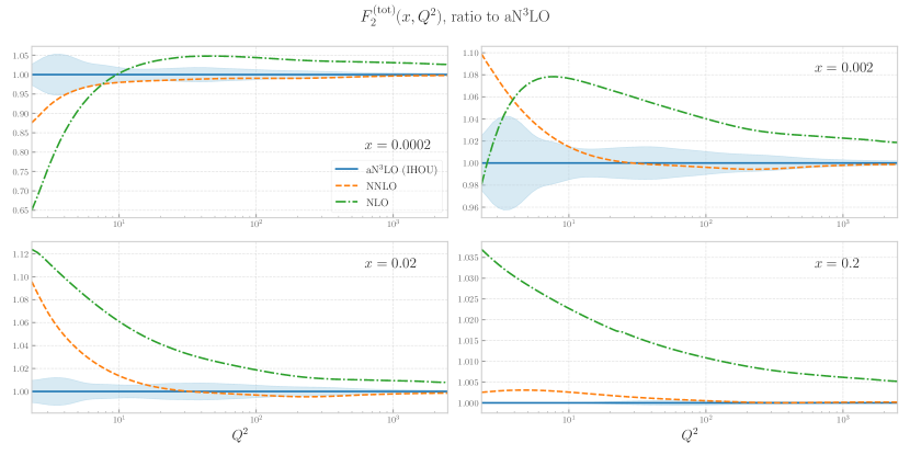
Figure 3.6: Same as Fig. 3.5 for the inclusive structure function $F^{(\text{tot})}_{2}(x,Q^{2})$. Note the different scale on the $y$ axis.

An analogous study of perturbative convergence of the inclusive structure function is shown in Fig. 3.6 (note the different scale on the $y$ axis). Interestingly, the effect of the aN³LO corrections changes sign when going from $x=2\times 10^{-4}$ to larger values of $x$. In general, N³LO corrections are smaller at the inclusive level: specifically, aN³LO corrections to the inclusive structure function are below 2% for $Q^{2}\mathrel{\hbox to0.0pt{\lower 4.0pt\hbox{\hskip 1.0pt$\sim$}\hss}\raise 1.0pt\hbox{$>$}}10$ GeV², and at most of order 10% around the charm mass scale. The impact of the IHOUs on the heavy coefficient is further reduced due to the fact that charm contributes at most one quarter of the total structure function. Consequently, the aN³LO correction to the NNLO result is now larger than the IHOU in a significant kinematic region. This, together with the fact that aN³LO corrections are comparable or larger than typical experimental uncertainties on structure function data, motivates their inclusion in a global PDF determination.

3.3 N³LO corrections to hadronic processes

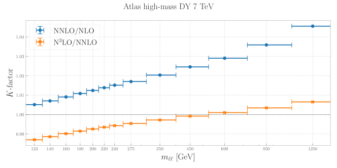
Figure 3.7: Ratio of the total NC Drell-Yan cross-section as a function of the NNLO/NLO and N³LO/NNLO calculations for the inclusive NC Drell-Yan cross-section in bins of $m_{\ell\ell}$, the invariant mass of the final-state dilepton pair, using the n3loxs code, integrated over all other kinematic variables. The $m_{\ell\ell}$ binning is chosen to be that of the ATLAS 7 TeV high-mass DY measurement [103]. The same PDF set is used in the numerator and denominator, namely NNPDF4.0 NNLO (for NNLO/NLO) and aN³LO (for N³LO/NNLO).

N³LO corrections to the total cross-section for inclusive neutral- (NC) and charged-current (CC) Drell-Yan production [11, 12] are available through the n3loxs public code [8], both for on-shell $W$ and $Z$ and as a function of the dilepton invariant mass $m_{\ell\ell}$. Differential distributions at the level of leptonic observables for the same processes have also been computed [18, 19], but are not publicly available. No N³LO calculations are available for other processes included in the NNPDF4.0 dataset.

The ratio of the NC total cross-section evaluated at two subsequent perturbative orders with a fixed set of PDFs, chosen as NNPDF4.0NNLO is shown in Fig. 3.7. Results are shown in the high-mass region, as a function of $m_{\ell\ell}$, with the same binning as the ATLAS 7 TeV measurement [103]. Perturbative convergence is apparent, with the N³LO/NNLO ratio closer to unity and smoother than its NNLO/NLO counterpart: while NNLO corrections range between $+0.5\%$ and $+4\%$, at N³LO they are reduced to $-1.2\%$ and $+0.5\%$.

Total cross-section data are obtained by extrapolating measurements performed in a fiducial region. Whereas for NC Drell-Yan production in the central rapidity region and for dilepton invariant masses around the $Z$-peak, the N³LO/NNLO cross-section ratio depends only mildly on the dilepton rapidity $y_{\ell\ell}$ [18, 19], it is unclear whether this is the case also off-peak or at very large and very small rapidities. Hence, the inclusion of N³LO corrections for hadronic processes is, at present, not fully reliable. We have consequently not included them in our default determination, but only in a dedicated variant, with the goal of assessing their impact.

The datasets for which N³LO corrections have been included in this variant are listed in Table 3.1. We include the high-mass NC cross section, the $Z$ rapidity distribution in the central rapidity region for on-shell $Z$-production, and the total $W$ and $Z$ cross-sections. For all these processes the N³LO cross-section is determined by multiplying the NNLO result by a $K$-factor determined using a fixed underlying PDF set, namely the aN³LO NNPDF4.0 PDF set to be discussed in Sect. 4 below. Specifically, for the rapidity distribution we take the same fixed $K$-factor as for the total cross-section. We do not include off-shell or double-differential rapidity distributions (specifically from CMS), off-forward rapidity distributions (specifically from LHCb) and low-mass total cross-sections, for all of which the approximation of assuming the $K$-factor to be independent of rapidity and/or amenable to fiducial extrapolation is even less reliable. The datasets are labeled as in Table 2.4 of Ref. [37] .

Dataset	Ref.	$n_{\rm dat}$	Kin1	Kin2 [GeV]
ATLAS high-mass DY 7 TeV	[103]	13	$|\eta_{\ell}|\leq 2.1$	$116\leq m_{\ell\ell}\leq 1500$
ATLAS $Z$ 7 TeV ($\mathcal{L}=35$ pb-1)	[104]	8	$|\eta_{\ell},y_{Z}|\leq 3.2$	$Q=m_{Z}$
ATLAS $Z$ 7 TeV ($\mathcal{L}=4.6$ fb-1)	[105]	39	$|\eta_{\ell},y_{Z}|\leq 2.5,3.6$	$Q=m_{Z}$
ATLAS $\sigma_{W,Z}^{\rm tot}$ 13 TeV	[106]	3	—	$Q=m_{W},m_{Z}$

Table 3.1: The LHC NC DY production datasets in NNPDF4.0 for which an N³LO $K$-factor has been included in a variant of the default aN³LO PDF determination (see Sect. 4). For each dataset we indicate the published references, the number of datapoints and the kinematic variables.

Despite the fact that we are not yet able to determine reliably N³LO corrections for currently available LHC measurements, we wish to include the full NNPDF4.0 dataset in our aN³LO PDF determination. To this purpose, we endow all data for which N³LO are not included with an extra uncertainty that accounts for the missing N³LO terms. This is estimated using the methodology of Refs. [35, 36], recently used in Ref. [38] to produce a variant of the NNPDF4.0 PDF sets that includes MHOUs.

Thus, when not including N³LO corrections to the hard cross-section, the theory prediction is evaluated by combining aN³LO evolution with the NNLO cross sections. The prediction is then supplemented with a theory covariance matrix, computed varying the renormalization scale $\mu_{R}$ using a three-point prescription [35, 36]:

$$\text{cov}^{\rm NNLO}_{mn}=\frac{1}{2}\left(\Delta_{m}(+)\Delta_{n}(+)+\Delta_{m}(-)\Delta_{n}(-)\right),$$ (3.8)

analogous to Eq. (3.6), but now with $\Delta_{m}(\pm)$ the shift in the prediction for the $m$-th data point obtained by replacing the coefficient functions with those obtained by performing upper or lower renormalization scale variation using the methodology of Ref. [36] (as implemented and discussed in Ref. [38], Eq. (2.9)). This MHOU covariance matrix is then added to the IHOU covariance matrix as a further term on the right-hand side of Eq. (2.20).

The impact of this uncertainty is shown in Fig. 3.8, where we show for all hadronic datasets the square root of the diagonal entries of the MHOU covariance matrix Eq. (3.8), compared to those of the IHOU covariance matrix Eq. (2.20), and to the experimental uncertainties, all normalized to the central theory prediction. The MHOU is generally larger than the IHOU, indicating that the missing N³LO terms in the hard cross-sections are larger than the IHOU uncertainty in N³LO perturbative evolution. The experimental uncertainties are generally larger still.

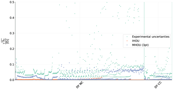
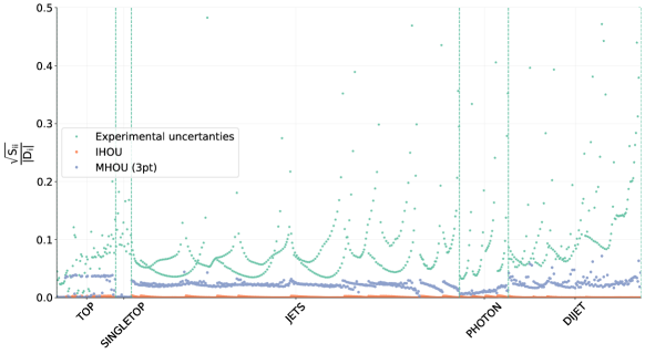
Figure 3.8: Same as Fig. 3.3 now comparing the IHOU from Eq. (2.20) with the MHOU from Eq. (3.8) due to the missing N³LO correction to the matrix element. Results are shown for all hadronic data in the NNPDF4.0 dataset: specifically Drell-Yan (top) and top pair, single top, single-inclusive jet, prompt photon and dijet production (bottom).

In addition to the NNPDF4.0 aN³LO baseline PDF set obtained in this manner, we will also produce a NNPDF4.0 MHOU aN³LO set, in analogy to the NLO and NNLO MHOU sets recently presented in Ref. [38]. For this set, MHOUs on both perturbative evolution and on the hard matrix elements are included using the methodology of Refs. [35, 36] with a theory covariance matrix determined performing combined correlated renormalization and factorization scale variations with a 7-point prescription, as discussed in detail in Ref. [38]. In this case, we simply perform scale variation on the expressions at the order at which they are being computed, namely aN³LO for anomalous dimensions and DIS coefficient functions and NNLO for hadronic processes. The scale variation then is automatically larger and suitable deweights processes for which N³LO corrections are not available. The possibility of simultaneously including in a PDF determination processes for which theory predictions are only available at different perturbative orders is an advantage of the inclusion of MHOUs in the PDF determination, as already pointed out in Refs. [107, 108].

4 NNPDF4.0 at aN³LO

We now present the aN³LO NNPDF4.0 PDF sets. They have been obtained by using the dataset and methodology discussed in [37] and used for the construction of the LO, NLO, and NNLO NNPDF4.0 presented there, now extended to aN³LO. The aN³LO results are obtained using the approximate N³LO splitting function of Sect. 2, the exact massless and approximate massive N³LO coefficient functions of Sect. 3.1, and NNLO hadronic cross-sections supplemented by an extra uncertainty as per Sect. 3.3.

Theoretical predictions are obtained using the new theory pipeline of Ref. [70], which relies on the EKO evolution code [40] and on the YADISM DIS module [41]. As discussed in Sect. 3.2, this pipeline in particular includes a new FONLL implementation, that differs from the previous one by subleading terms. A further small difference in comparison to Ref. [37] is the correction of a few minor bugs in the data implementation. The overall impact of all these changes was assessed in Appendix A of Ref. [109], and was found to be very limited, so that the new and old implementations can be considered equivalent, and the PDF sets presented here can be considered the extension to aN³LO of the NNPDF4.0 PDF sets of Ref. [37].

In addition to the default NNPDF4.0 aN³LO PDF determination, we also present an aN³LO PDF determination that includes MHOUs on all the theory predictions used in the PDF determination. This is constructed using the same methodology recently used to produce the NNPDF4.0MHOU NNLO PDF set in Ref. [38]. In order to be able to discuss perturbative convergence and the impact of MHOUs we will also present a NNPDF4.0MHOU NLO PDF set constructed using the same methodology, and exactly the same dataset as the default NNPDF4.0 NLO PDF set (which differs from the NNPDF4.0 NNLO dataset).

We finally construct two variants of the aN³LO PDF sets (both with and without MHOUs) with modified N³LO theory. In a first variant, we replace our own approximation to the N³LO anomalous dimensions, discussed in Sect. 2, with that of Refs. [28, 29, 30]. In the second variant, we will also include N³LO corrections for the processes listed in Tab. 3.1, as discussed in Sect. 3.3.

We first assess the fit quality, then present the PDFs and their uncertainties, and study perturbative convergence and the effect on it of the inclusion of MHOUs. We then specifically study the impact of aN³LO corrections on intrinsic charm. We then turn to the variants, and finally compare our results to the recent MSHT20 aN³LO PDFs.

4.1 Fit quality

Tables 4.1-4.4 display the number of data points and the $\chi^{2}$ per data point obtained in the NLO, NNLO, and aN³LO NNPDF4.0 fits with and without MHOUs. In Table 4.1 the datasets are grouped according to the process categorisation used in Ref. [38]. Results for individual datasets are displayed in Table 4.2, (NC and CC DIS), in Table 4.3 (NC and CC DY), and in Table 4.4 (top pairs, single-inclusive jets, dijets, isolated photons, and single top). The naming of the datasets follows Ref. [37]. The value of the total $\chi^{2}$ per data point is also shown as a function of the perturbative order in Fig. 4.1.

	NLO			NNLO			aN3LO
Dataset	$N_{\rm dat}$	no MHOU	MHOU	$N_{\rm dat}$	no MHOU	MHOU	$N_{\rm dat}$	no MHOU	MHOU
DIS NC	1980	1.30	1.22	2100	1.22	1.20	2100	1.22	1.20
DIS CC	988	0.92	0.87	989	0.90	0.90	989	0.91	0.92
DY NC	667	1.49	1.32	736	1.20	1.15	736	1.17	1.16
DY CC	193	1.31	1.27	157	1.45	1.37	157	1.37	1.36
Top pairs	64	1.90	1.24	64	1.27	1.43	64	1.23	1.41
Single-inclusive jets	356	0.86	0.82	356	0.94	0.81	356	0.84	0.83
Dijets	144	1.55	1.81	144	2.01	1.71	144	1.78	1.67
Prompt photons	53	0.58	0.47	53	0.76	0.67	53	0.72	0.68
Single top	17	0.35	0.34	17	0.36	0.38	17	0.35	0.36
Total	4462	1.24	1.16	4616	1.17	1.13	4616	1.15	1.14

Table 4.1: The number of data points and the $\chi^{2}$ per data point obtained in the NLO, NNLO, and aN³LO NNPDF4.0 fits without and with MHOUs, see text for details. The datasets are grouped according to the same process categorisation as that used in Ref. [38].

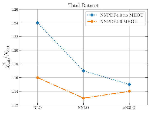
Figure 4.1: The values of the total $\chi^{2}$ per data point in the NNPDF4.0 NLO, NNLO, and aN³LO fits without and with MHOUs.

	NLO			NNLO			aN3LO
Dataset	$N_{\rm dat}$	no MHOU	MHOU	$N_{\rm dat}$	no MHOU	MHOU	$N_{\rm dat}$	no MHOU	MHOU
NMC $F_{2}^{d}/F_{2}^{p}$	121	0.87	0.86	121	0.87	0.88	121	0.88	0.88
NMC $\sigma^{{\rm NC},p}$	203	1.82	1.30	204	1.57	1.33	204	1.57	1.36
SLAC $F_{2}^{p}$	33	1.64	0.74	33	0.91	0.68	33	0.93	0.72
SLAC $F_{2}^{d}$	34	0.90	0.68	34	0.61	0.54	34	0.62	0.58
BCDMS $F_{2}^{p}$	333	1.62	1.24	333	1.40	1.29	333	1.39	1.40
BCDMS $F_{2}^{d}$	248	1.05	1.00	248	1.01	0.99	248	1.04	1.03
HERA I+II $\sigma_{\rm NC}\ e^{-}p$	159	1.44	1.40	159	1.40	1.39	159	1.45	1.40
HERA I+II $\sigma_{\rm NC}\ e^{+}p$ ($E_{p}=460$ GeV)	192	1.12	1.05	204	1.09	1.04	204	1.07	1.05
HERA I+II $\sigma_{\rm NC}\ e^{+}p$ ($E_{p}=575$ GeV)	236	0.85	0.84	254	0.93	0.88	254	0.87	0.88
HERA I+II $\sigma_{\rm NC}\ e^{+}p$ ($E_{p}=820$ GeV)	54	1.15	0.85	70	1.12	0.95	70	0.96	0.86
HERA I+II $\sigma_{\rm NC}\ e^{+}p$ ($E_{p}=920$ GeV)	317	1.30	1.21	377	1.31	1.25	377	1.27	1.24
HERA I+II $\sigma_{\rm NC}^{c}$	24	2.18	1.40	37	1.96	1.75	37	1.86	1.57
HERA I+II $\sigma_{\rm NC}^{b}$	26	1.42	1.05	26	1.44	1.11	26	1.26	1.07
CHORUS $\sigma_{CC}^{\nu}$	416	0.96	0.95	416	0.96	0.97	416	0.97	0.98
CHORUS $\sigma_{CC}^{\bar{\nu}}$	416	0.90	0.88	416	0.88	0.87	416	0.88	0.88
NuTeV $\sigma_{CC}^{\nu}$ (dimuon)	39	0.24	0.22	39	0.33	0.33	39	1.27	1.28
NuTeV $\sigma_{CC}^{\bar{\nu}}$ (dimuon)	36	0.43	0.35	37	0.56	0.64	37	0.63	0.59
HERA I+II $\sigma_{\rm CC}\ e^{-}p$	42	1.34	1.19	42	1.25	1.29	42	1.29	1.34
HERA I+II $\sigma_{\rm CC}\ e^{+}p$	39	1.26	1.22	39	1.23	1.25	39	1.27	1.28

Table 4.2: Same as Table 4.1 for DIS NC (top) and DIS CC (bottom) datasets.

	NLO			NNLO			aN3LO
Dataset	$N_{\rm dat}$	no MHOU	MHOU	$N_{\rm dat}$	no MHOU	MHOU	$N_{\rm dat}$	no MHOU	MHOU
E866 $\sigma^{d}/2\sigma^{p}$ (NuSea)	15	0.59	0.47	15	0.52	0.51	15	0.53	0.51
E866 $\sigma^{p}$ (NuSea)	89	1.33	0.86	29	1.59	1.00	29	1.08	1.03
E605 $\sigma^{d}/2\sigma^{p}$ (NuSea)	85	0.43	0.42	85	0.46	0.45	85	0.45	0.45
E906 $\sigma^{d}/2\sigma^{p}$ (SeaQuest)	6	1.47	0.74	6	0.97	0.90	6	0.82	0.88
CDF $Z$ differential	28	1.23	1.24	28	1.23	1.18	28	1.23	1.22
D0 $Z$ differential	28	0.69	0.71	28	0.64	0.64	28	0.64	0.63
ATLAS low-mass DY 7 TeV	4	0.69	0.66	6	0.88	0.78	6	0.78	0.76
ATLAS high-mass DY 7 TeV	5	1.74	1.66	5	1.60	1.67	5	1.64	1.68
ATLAS $Z$ 7 TeV ($\mathcal{L}=35$ pb-1)	8	0.67	0.44	8	0.58	0.57	8	0.56	0.61
ATLAS $Z$ 7 TeV ($\mathcal{L}=4.6$ fb-1) CC	16	3.82	2.99	24	1.80	1.68	24	1.66	1.69
ATLAS $Z$ 7 TeV ($\mathcal{L}=4.6$ fb-1) CF	15	1.77	1.22	15	1.07	1.02	15	1.02	0.99
ATLAS low-mass DY 2D 8 TeV	47	1.38	0.94	60	1.23	1.08	60	1.17	1.13
ATLAS high-mass DY 2D 8 TeV	48	1.52	1.38	48	1.11	1.08	48	1.09	1.09
ATLAS $\sigma_{Z}^{\rm tot}$ 13 TeV	1	0.12	0.41	1	0.24	0.60	1	0.24	0.66
ATLAS $Z$ $p_{T}$ 8 TeV ($p_{T},m_{\ell\ell}$)	41	1.08	0.91	44	0.91	0.91	44	0.89	0.89
ATLAS $Z$ $p_{T}$ 8 TeV ($p_{T},y_{Z}$)	28	0.87	0.52	48	0.90	0.70	48	0.77	0.68
CMS DY 2D 7 TeV	88	1.29	1.11	110	1.34	1.32	110	1.34	1.36
CMS $Z$ $p_{T}$ 8 TeV	28	1.66	1.47	28	1.40	1.41	28	1.35	1.39
LHCb $Z\to ee$ 7 TeV	9	1.47	1.18	9	1.65	1.53	9	1.48	1.46
LHCb $Z\to\mu$ 7 TeV	15	1.03	0.87	15	0.80	0.73	15	0.77	0.73
LHCb $Z\to ee$ 8 TeV	17	1.58	1.38	17	1.24	1.26	17	1.31	1.27
LHCb $Z\to\mu$ 8 TeV	15	1.25	1.06	15	1.44	1.59	15	1.60	1.60
LHCb $Z\to ee$ 13 TeV	15	1.68	1.60	15	1.72	1.80	15	1.78	1.76
LHCb $Z\to\mu\mu$ 13 TeV	16	1.10	1.11	16	0.94	0.99	16	0.99	0.94
D0 $W$ muon asymmetry	8	2.42	2.17	9	1.86	1.95	9	2.07	2.03
ATLAS $W$ 7 TeV ($\mathcal{L}=35$ pb-1)	22	1.20	1.13	22	1.11	1.12	22	1.09	1.12
ATLAS $W$ 7 TeV ($\mathcal{L}=4.6$ fb-1)	22	2.18	2.13	22	2.08	2.16	22	2.16	2.10
ATLAS $\sigma_{W}^{\rm tot}$ 13 TeV	2	0.16	0.54	2	1.21	1.60	2	1.38	1.67
ATLAS $W^{+}$+jet 8 TeV	15	0.26	0.28	15	0.79	0.79	15	0.73	0.73
ATLAS $W^{-}$+jet 8 TeV	15	0.98	1.27	15	1.49	1.45	15	1.41	1.41
CMS $W$ electron asymmetry 7 TeV	11	0.92	1.03	11	0.84	0.85	11	0.82	0.86
CMS $W$ muon asymmetry 7 TeV	11	2.03	1.77	11	1.71	1.73	11	1.70	1.71
CMS $W$ rapidity 8 TeV	22	0.93	0.74	22	1.33	1.03	22	1.11	1.08
LHCb $W\to\mu$ 7 TeV	14	1.63	1.26	14	2.78	1.99	14	2.12	2.03
LHCb $W\to\mu$ 8 TeV	14	0.60	0.44	14	0.97	0.92	14	0.80	0.84

Table 4.3: Same as Table 4.1 for DY NC (top) and DY CC (bottom) datasets.

	NLO			NNLO			aN3LO
Dataset	$N_{\rm dat}$	no MHOU	MHOU	$N_{\rm dat}$	no MHOU	MHOU	$N_{\rm dat}$	no MHOU	MHOU
ATLAS $\sigma_{tt}^{\rm tot}$ 7 TeV	1	10.4	0.96	1	4.50	2.40	1	2.78	2.05
ATLAS $\sigma_{tt}^{\rm tot}$ 8 TeV	1	1.74	0.59	1	0.02	0.03	1	0.04	0.08
ATLAS $\sigma_{tt}^{\rm tot}$ 13 TeV ($\mathcal{L}$=139 fb-1)	1	3.82	0.96	1	0.49	0.41	1	0.51	0.44
ATLAS $t\bar{t}~{}\ell$+jets 8 TeV ($1/\sigma d\sigma/dy_{t}$)	4	4.16	1.79	4	3.13	3.70	4	2.98	3.64
ATLAS $t\bar{t}~{}\ell$+jets 8 TeV ($1/\sigma d\sigma/dy_{t\bar{t}}$)	4	8.93	3.73	4	4.50	5.80	4	4.26	4.92
ATLAS $t\bar{t}~{}2\ell$ 8 TeV ($1/\sigma d\sigma/dy_{t\bar{t}}$)	4	1.94	1.76	4	1.60	1.86	4	1.66	1.80
CMS $\sigma_{tt}^{\rm tot}$ 5 TeV	1	0.61	0.73	1	0.02	0.01	1	0.03	0.02
CMS $\sigma_{tt}^{\rm tot}$ 7 TeV	1	5.27	1.30	1	1.01	0.50	1	0.60	0.34
CMS $\sigma_{tt}^{\rm tot}$ 8 TeV	1	3.50	0.85	1	0.26	0.17	1	0.21	0.10
CMS $\sigma_{tt}^{\rm tot}$ 13 TeV	1	0.75	0.26	1	0.06	0.01	1	0.04	0.05
CMS $t\bar{t}~{}\ell$+jets 8 TeV ($1/\sigma d\sigma/dy_{t\bar{t}}$)	9	1.87	1.59	9	1.21	1.59	9	1.31	1.52
CMS $t\bar{t}$ 2D $2\ell$ 8 TeV ($1/\sigma d\sigma/dy_{t}dm_{t\bar{t}}$)	15	2.03	1.89	15	1.30	1.25	15	1.28	1.37
CMS $t\bar{t}~{}2\ell$ 13 TeV ($d\sigma/dy_{t}$)	10	0.78	0.69	10	0.51	0.59	10	0.55	0.60
CMS $t\bar{t}~{}\ell$+jet 13 TeV ($d\sigma/dy_{t}$)	11	0.66	0.25	11	0.60	0.66	11	0.52	0.71
ATLAS incl. jets 8 TeV, $R=0.6$	171	0.67	0.74	171	0.68	0.64	171	0.68	0.64
CMS incl. jets 8 TeV	185	0.95	0.83	185	1.19	0.95	185	0.97	0.99
ATLAS dijets 7 TeV, $R=0.6$	90	1.47	1.72	90	2.14	1.69	90	1.76	1.63
CMS dijets 7 TeV	54	1.57	2.01	54	1.79	1.74	54	1.84	1.78
ATLAS isolated $\gamma$ prod. 13 TeV	53	0.57	0.47	53	0.76	0.67	53	0.72	0.68
ATLAS single $t$ $R_{t}$ 7 TeV	1	0.43	0.29	1	0.50	0.57	1	0.51	0.58
ATLAS single $t$ $R_{t}$ 13 TeV	1	0.04	0.03	1	0.06	0.07	1	0.06	0.07
ATLAS single $t$ 7 TeV ($1/\sigma d\sigma/dy_{t}$)	3	0.83	0.84	3	0.96	0.94	3	0.97	0.97
ATLAS single $t$ 7 TeV ($1/\sigma d\sigma/dy_{\bar{t}}$)	3	0.06	0.06	3	0.06	0.06	3	0.06	0.06
ATLAS single $t$ 8 TeV ($1/\sigma d\sigma/dy_{t}$)	3	0.38	0.31	3	0.25	0.26	3	0.22	0.24
ATLAS single $t$ 8 TeV ($1/\sigma d\sigma/dy_{\bar{t}}$)	3	0.19	0.21	3	0.19	0.19	3	0.20	0.20
CMS single $t$ $\sigma_{t}+\sigma_{\bar{t}}$ 7 TeV	1	0.89	0.88	1	0.74	0.84	1	0.39	0.43
CMS single $t$ $R_{t}$ 8 TeV	1	0.15	0.08	1	0.18	0.20	1	0.18	0.21
CMS single $t$ $R_{t}$ 13 TeV	1	0.33	0.27	1	0.36	0.38	1	0.36	0.38

Table 4.4: Same as Table 4.1 for (from top to bottom) top pair, single-inclusive jet, isolated photon and single top production datasets.

The NLO and NNLO results without MHOUs are obtained using the NLO and NNLO NNPDF4.0 PDF sets [37]. The NNLO result with MHOUs is obtained using the NNPDF4.0MHOU NNLO set from Ref. [38], while, as already mentioned, the NNPDF4.0MHOU NLO presented here for the first time uses an identical methodology to NNPDF4.0MHOU NNLO [38], but the same dataset as NNPDF4.0 NLO [37]. Hence, the datasets with and without MHOU are always the same, but the NLO and NNLO datasets are not the same but rather follow Ref. [37]. The N³LO dataset is the same as NNLO. In all cases, the theoretical predictions entering the computation of the $\chi^{2}$ are obtained with the new theory pipeline. The covariance matrix, whenever needed, is computed as described in Sect. 4.1 of Ref. [38]. The N³LO predictions are computed with the aforementioned aN³LO PDF sets. These are based on the same datasets and kinematic cuts as the NNPDF4.0 NNLO PDF sets, use the theoretical predictions discussed in Sects. 2-3, and are supplemented with a IHOU covariance matrix as discussed in Sects. 2.2-3.1 and a MHOU for hadronic processes for which N³LO hard cross sections are not available as discussed in Sect. 3.3.

Table 4.1 and Fig. 4.1 show that without MHOUs fit quality improves as the perturbative order increases. On the other hand, when MHOUs are included, fit quality becomes independent of perturbative order within uncertainties (note that, with $N_{\rm dat}=4462$, $\sigma_{\chi^{2}}=0.03$). This means that the MHOU covariance matrix estimated through scale variation is correctly reproducing the true MHOUs. Also, at aN³LO the fit quality is the same within uncertainties irrespective of whether MHOUs are included or not. This strongly suggests that within current experimental uncertainties, the current methodology and the current dataset the perturbative expansion has converged, meaning that inclusion of higher-order QCD correction beyond N³LO would not lead to a further improvement in fit quality to current data.

4.2 Parton distributions

We now examine the NNPDF4.0 aN³LO parton distributions. We compare the NLO, NNLO and aN³LO NNPDF4.0 PDFs, obtained without and with inclusion of MHOUs, in Figs. 4.2-4.3 and in Figs. 4.4-4.5, respectively. Specifically, we show the up, antiup, down, antidown, strange, antistrange, charm and gluon PDFs at $Q=100$ GeV, normalized to the aN³LO result, as a function of $x$ in logarithmic and linear scale. Error bands correspond to one sigma PDF uncertainties, which do (MHOU sets) or do not (no MHOU sets) include MHOUs on all theory predictions used in the fit. The PDF sets, with and without MHOUs, are the same used to compute the values of the $\chi^{2}$ in Tables 4.1-4.4.

The excellent perturbative convergence seen in the fit quality is also manifest at the level of PDFs. In particular, the NNLO PDFs are either very close to or indistinguishable from their aN³LO counterparts. Inclusion of MHOUs further improves the consistency between NNLO and aN³LO PDFs, which lie almost on top of each other. This means that the NNLO PDFs are made more accurate by the inclusion of MHOUs, and that the aN³LO PDFs have converged, in the sense discussed above. Exceptions to this stability are the charm and gluon PDFs, for which aN³LO corrections have a sizeable impact. In the case of charm, they lead to an enhancement of the central value of about 4% for $x\sim 0.05$; in the case of gluon, to a suppression of about 2-3% for $x\sim 0.005$. In both cases, inclusion of MHOUs leads to an increase in PDF uncertainties by about 1-2%. This makes the NNLO and aN³LO charm PDFs with MHOUs compatible within uncertainties, and the NNLO and aN³LO gluon PDFs with MHOU almost compatible.

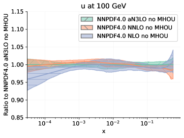
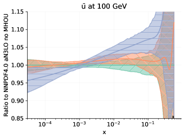
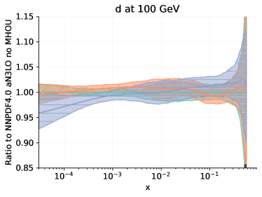
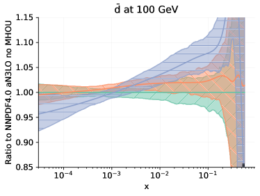
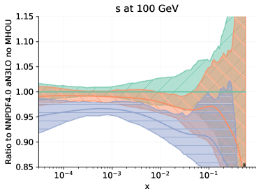
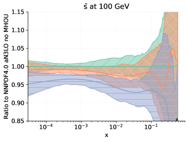
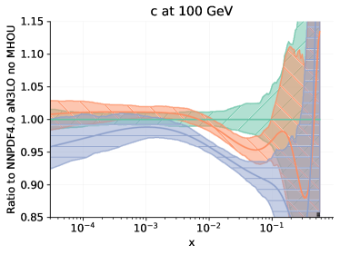
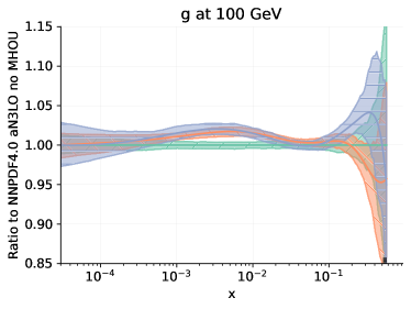
Figure 4.2: The NLO, NNLO and aN³LO NNPDF4.0 PDFs at $Q=100$ GeV. We display the up, antiup, down, antidown, strange, antistrange, charm and gluon PDFs normalized to the aN³LO result. Error bands correspond to one sigma PDF uncertainties, not including MHOUs on the theory predictions used in the fit.

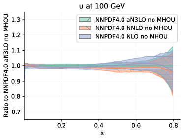
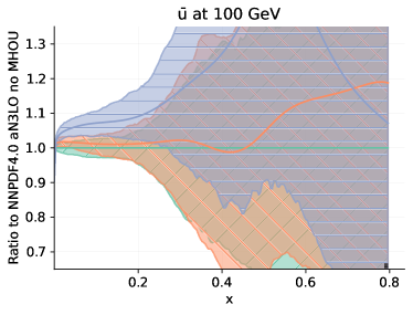
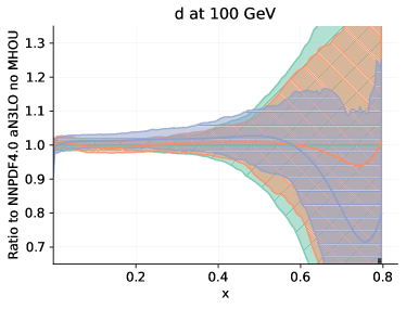
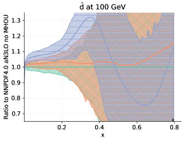
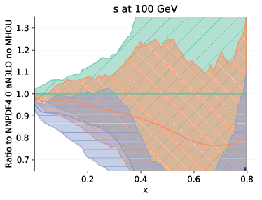
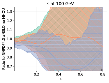
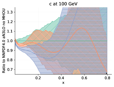
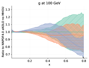
Figure 4.3: Same as Fig. 4.2 in linear scale.

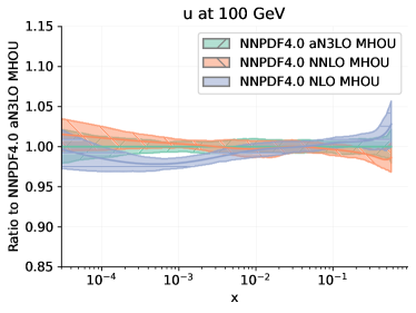
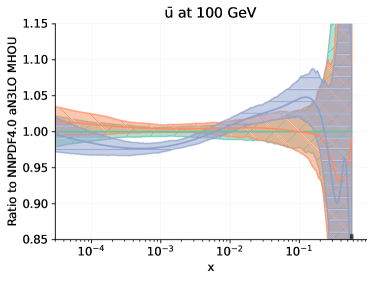
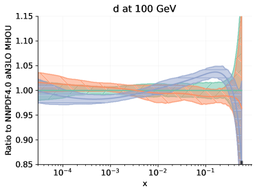
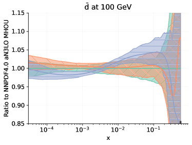
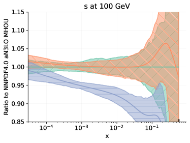
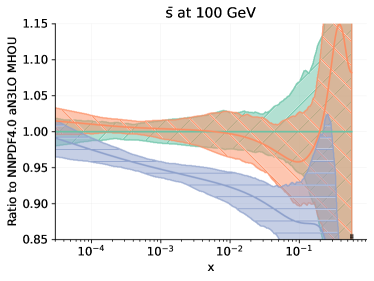
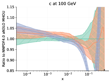
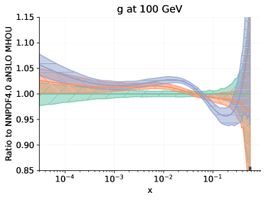
Figure 4.4: Same as Fig. 4.2 for NNPDF4.0MHOU PDF sets. Error bands correspond to one sigma PDF uncertainties also including MHOUs on the theory predictions used in the fit.

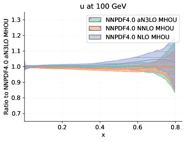
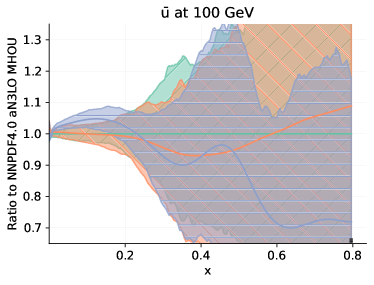
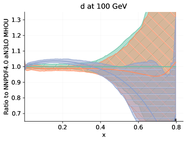
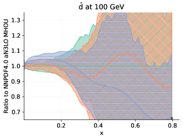
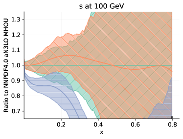
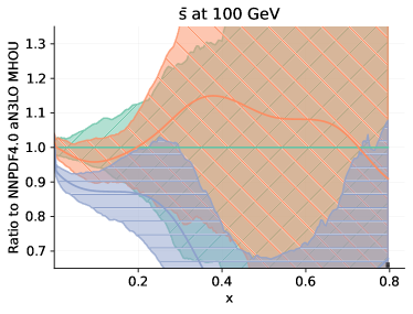
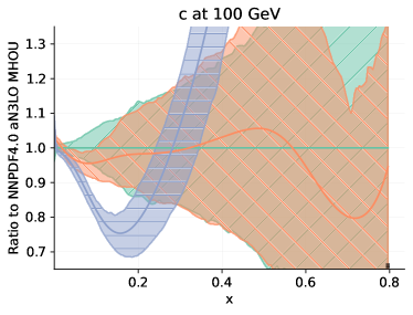
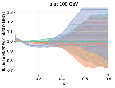
Figure 4.5: Same as Fig. 4.4 in linear scale.

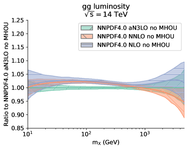
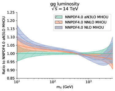
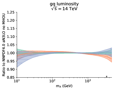
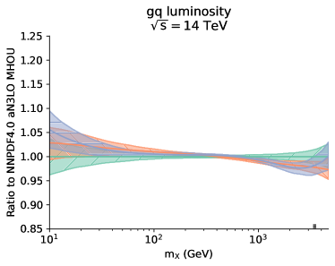
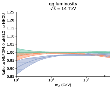
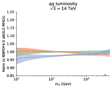
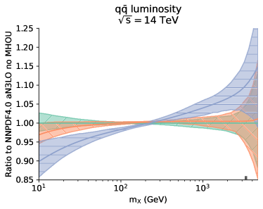
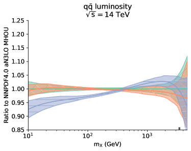
Figure 4.6: The gluon-gluon, gluon-quark, quark-quark, and quark-antiquark parton luminosities as a function of $m_{X}$ at $\sqrt{s}=14$ TeV, computed with NLO, NNLO and aN³LO NNPDF4.0 PDFs without MHOUs (left) and with MHOUs (right), all shown as a ratio to the respective aN³LO results. Uncertainties are as in Figs. 4.2-4.4

Figure 4.6 presents a comparison similar to that of Figs. 4.2-4.4 for the gluon-gluon, gluon-quark, quark-quark, and quark-antiquark parton luminosities. These are shown integrated in rapidity as a function of the invariant mass of the final state $m_{X}$ for a center-of-mass energy $\sqrt{s}=14$ TeV. Their definition follows Eqs. (1)-(4) of Ref. [110].

As already observed for PDFs, perturbative convergence is excellent, and improves upon inclusion of MHOUs. The NNLO and aN³LO results are compatible within uncertainties for the gluon-quark, quark-quark, and quark-antiquark luminosities. Some differences are seen for the gluon-gluon luminosity, consistent with the differences seen in the gluon PDF. Specifically, the aN³LO corrections lead to a suppression of the gluon-gluon luminosity of 2-3% for $m_{X}\sim 100$ GeV. This effect is somewhat compensated by an increase in uncertainty of about 1% upon inclusion of MHOUs. Indeed, the NNLO and aN³LO gluon-gluon luminosities for $m_{X}\sim 100$ GeV differ by about $2.5\sigma$ without MHOU, but become almost compatible within uncertainties when MHOUs are included.

All in all, these results show that aN³LO corrections are generally small, except for the gluon PDF, and that at aN³LO the perturbative expansion has all but converged, with NNLO and aN³LO PDFs very close to each other, especially upon inclusion of MHOUs. They also show that MHOUs generally improve the accuracy of PDFs, though at aN³LO they have a very small impact. The phenomenological consequences of this state of affairs will be further discussed in Sect. 5.

4.3 PDF uncertainties

We now take a closer look at PDF uncertainties. In Fig. 4.7 we display one sigma uncertainties for the NNPDF4.0 NLO, NNLO, and aN³LO PDFs with and without MHOUs at $Q=100$ GeV. All uncertainties are normalized to the central value of the NNPDF4.0 aN³LO PDF set with MHOUs. The NLO uncertainty is generally the largest of all in the absence of MHOUs, and for quark distributions the smallest once MHOUs are included. All other uncertainties, at NNLO and aN³LO, with and without MHOUs, are quite similar to each other, especially for quark PDFs. The fact that upon inclusion of an extra source of uncertainty, namely the MHOU, PDF uncertainties are reduced (at NLO) or unchanged (at NNLO and aN³LO) may look counter-intuitive. However, as already pointed out in Refs. [34, 111, 38], this can be understood to be a consequence of the increased compatibility of the data due to inclusion of MHOUs and of higher-order perturbative corrections.

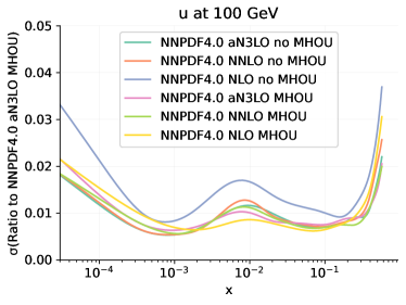
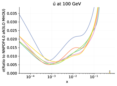
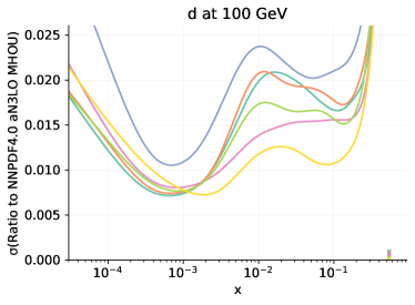
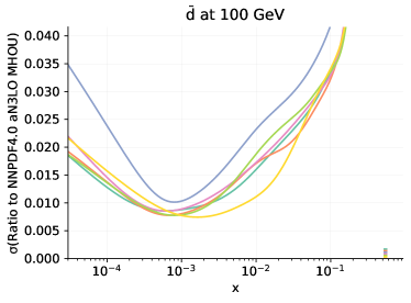
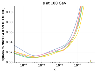
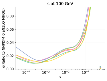
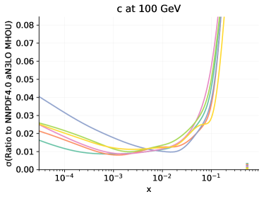
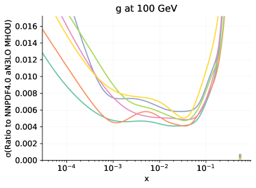
Figure 4.7: Relative one sigma uncertainties for the PDFs shown in Figs. 4.2-4.4. All uncertainties are normalized to the central value of the NNPDF4.0 aN³LO set with MHOUs.

The impact of MHOUs on NLO and NNLO PDFs was extensively assessed in Ref. [38]. In a similar vein, here we focus on the impact of MHOUs on aN³LO PDFs. To this purpose, in Fig. 4.8 we compare the NNPDF4.0 aN³LO PDFs with and without MHOUs. The related comparison for parton luminosities is presented in Fig. 4.9. Again, aN³LO PDFs and luminosities with and without MHOU are very compatible with each other. This evidence reinforces the expectation that perturbative corrections beyond N³LO will not alter PDFs significantly, at least with current data and methodology.

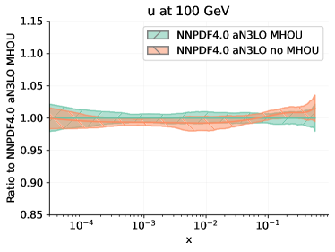
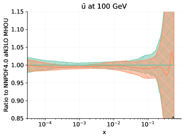
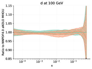
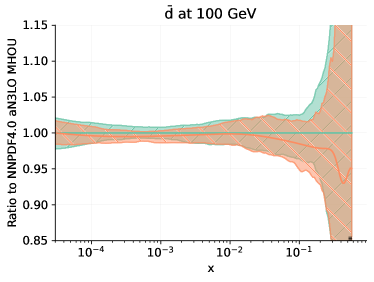
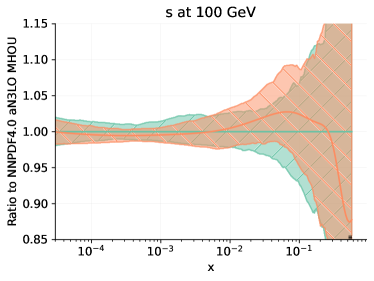
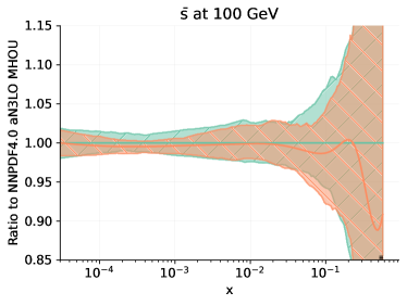
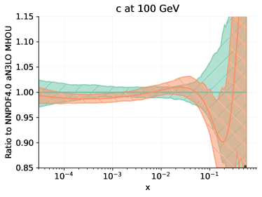
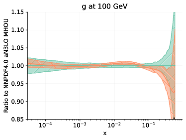
Figure 4.8: Same as Figs. 4.2-4.4, now comparing NNPDF4.0 aN³LO PDFs without and with MHOUs.

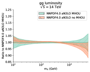
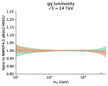
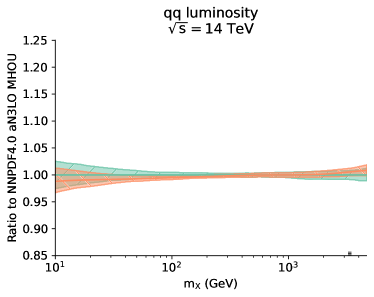
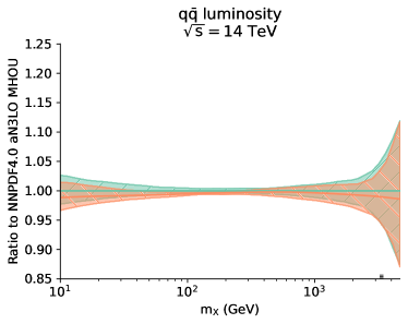
Figure 4.9: Same as Fig. 4.6, now comparing NNPDF4.0 aN³LO PDFs without and with MHOUs.

In analogy with Ref. [38], we also compare the $\phi$ estimator introduced in Ref. [112] (see Eq. (4.6) there). The estimator gives the ratio of the average correlated PDF uncertainty to the data uncertainty. As such, it provides an estimate of the consistency of the data: consistent data are combined by the underlying theory and lead to an uncertainty in the prediction which is smaller than that of the original data. The value of $\phi$ obtained in the NLO, NNLO, and aN³LO NNPDF4.0 fits with and without MHOUs (as in Table 4.1) is reported in Table 4.5. It is clear that $\phi$ converges to very similar values with the increase of the perturbative order and/or with inclusion of MHOUs for both the total dataset and for most of the data categories. This fact is further quantitative evidence of the excellent perturbative convergence of the PDF uncertainties.

	NLO		NNLO		N3LO
Dataset	no MHOU	MHOU	no MHOU	MHOU	no MHOU	MHOU
DIS NC	0.14	0.13	0.15	0.13	0.13	0.13
DIS CC	0.11	0.11	0.12	0.12	0.12	0.12
DY NC	0.19	0.17	0.18	0.17	0.17	0.18
DY CC	0.33	0.27	0.35	0.32	0.31	0.32
Top pairs	0.18	0.17	0.17	0.17	0.16	0.19
Single-inclusive jets	0.13	0.13	0.13	0.13	0.13	0.13
Dijets	0.10	0.10	0.11	0.10	0.10	0.10
Prompt photons	0.06	0.07	0.06	0.06	0.05	0.05
Single top	0.04	0.04	0.04	0.04	0.04	0.04
Total	0.18	0.15	0.16	0.15	0.15	0.15

Table 4.5: The $\phi$ uncertainty estimator for NNPDF4.0 PDFs at NLO, NNLO and aN³LO without and with MHOUs for the process categories as in Table 4.1.

4.4 Implications for intrinsic charm

The availability of the aN³LO PDFs discussed in Sects. 4.2-4.3 allows us to revisit and consolidate our recent results on intrinsic charm. Specifically, based on the NNPDF4.0 NNLO PDF determination, we have found evidence for intrinsic charm [113] and an indication for a non-vanishing valence charm component [114]. In these analyses, the dominant source of theory uncertainty was estimated to come from the matching conditions that are used in order to obtain PDFs in a three-flavor charm decoupling scheme from high-scale data, while MHOUs were assumed to be subdominant. The uncertainty in the matching conditions was in turn estimated by comparing results obtained using NNLO matching and the best available aN³LO matching conditions, both applied to NNLO PDFs.

It is now possible to improve these results on three counts. First, we can now fully include MHOUs. Second, we can consistently combine aN³LO matching conditions and aN³LO PDFs, and perform a consistent comparison of NNLO and aN³LO results. Finally, knowledge of aN³LO matching conditions themselves is now improved thanks to recent results [81] that were not available at the time of the analysis of Ref. [113]. We will specifically discuss the determination of the total intrinsic charm component and we do not consider the valence component, because effects of MHOUs and of the flavor scheme transformation are already very small at NNLO [114].

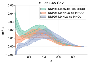
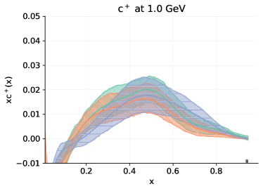
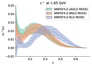
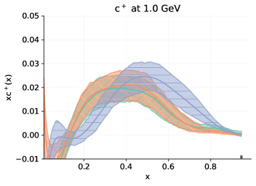
Figure 4.10: The total charm PDF, $xc^{+}(x,Q^{2})$, in the 4FNS at $Q=1.65$ GeV (left) and 3FNS (right), as obtained from the NNPDF4.0 NLO, NNLO, and aN³LO fits without (top) and with (bottom) MHOUs. Error bands correspond to one sigma PDF uncertainties. Note that in the 3FNS the charm PDF does not depend on scale.

To this purpose, in Fig. 4.10 we show the total charm PDF, $xc^{+}(x,Q^{2})$, in the 4FNS at $Q=1.65$ GeV and in the 3FNS, as obtained from using NNPDF4.0 NLO, NNLO and aN³LO without and with MHOUs. Note that in the 3FNS the charm PDF does not depend on scale. Error bands correspond to one sigma PDF uncertainties. The 4FNS results share the general features discussed in Sect. 4.2: the perturbative expansion converges nicely, with the aN³LO result very close to the NNLO. The convergence is further improved by the inclusion of MHOUs, which move the NNLO yet closer to the aN³LO. The 3FNS result is especially remarkable: whereas the combination of aN³LO matching with NNLO PDFs, used in Ref. [113] to conservatively estimate MHOUs, was somewhat unstable, now results display complete stability, and in particular the NNLO and aN³LO results completely coincide.

In order to assess the impact of MHOUs more clearly, in Fig. 4.11 we compare the total charm PDF in the 3FNS with and without MHOUs, respectively at NNLO and aN³LO. At NNLO MHOUs have a small but non-negligible impact on central values, with almost unchanged uncertainty, but at aN³LO they have essentially no impact, confirming the perturbative convergence of the result.

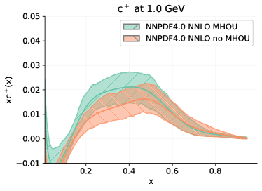
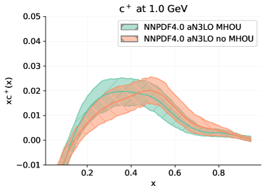
Figure 4.11: Same as Fig. 4.10, now comparing the total charm PDF in the 3FNS with and without MHOUs, respectively at NNLO (left) and aN³LO (right).

We thus proceed to a final re-assessment of the significance of intrinsic charm through the pull, defined as the central value divided by total uncertainty, using NNPDF4.0MHOU NNLO and aN³LO PDFs. We estimate the total uncertainty by adding in quadrature to the PDF uncertainty (which already includes the MHOU from the theory predictions used in the fit) a further theory uncertainty, taken equal to the difference between the central value at given perturbative order, and that at the previous perturbative order (so at NNLO from the difference to NLO, and so on). This now also includes the MHOU due to change in the matching from 4FNS to 3FNS, but also the shift in the 4FNS result that is in principle already accounted for by the MHOU. Also, it conservatively assumes that the shift between the current order and the next is equal to that from the previous order, rather than smaller. Results obtained with this conservative error estimate are shown in Fig. 4.12. It is clear that the significance of intrinsic charm is increased somewhat when going from NNLO to aN³LO. It is now also somewhat increased already at NNLO in comparison to the result of Ref. [113], despite the more conservative uncertainty estimate, thanks to the increased accuracy of MHOU PDFs and the consistent and improved treatment of matching aN³LO conditions. Indeed, local significance at the peak is now more than three sigma for the default fit.

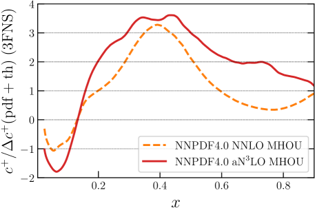
Figure 4.12: The pull (central value divided by total uncertainty) for the total charm PDF in the 3FNS obtained in the NNPDF4.0 NNLO and aN³LO fits with MHOUs.

4.5 Dependence on the treatment of aN³LO corrections.

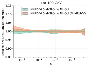
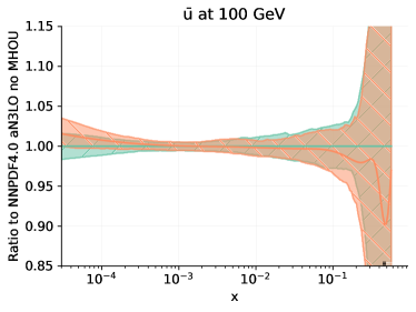
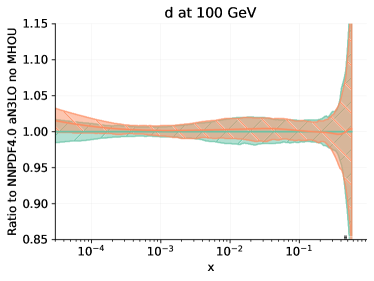
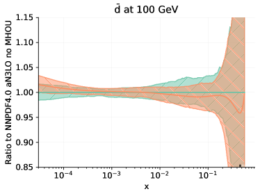
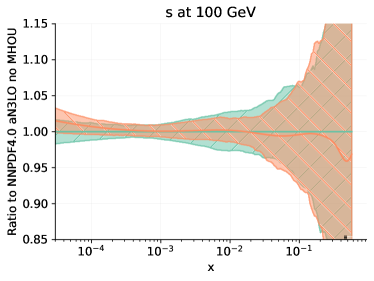
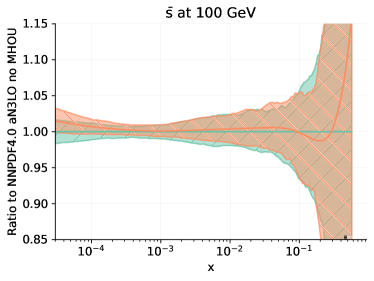
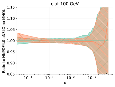
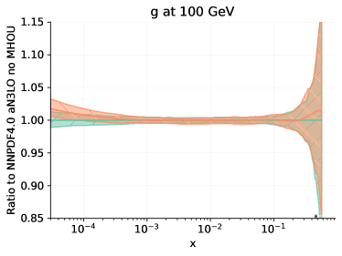
Figure 4.13: Same as Fig. 4.2, now comparing the NNPDF4.0 aN³LO PDFs and PDFs obtained using the FHMRUVV approximation to N³LO perturbative evolution.

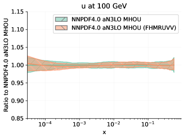
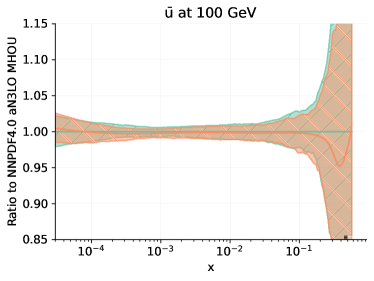
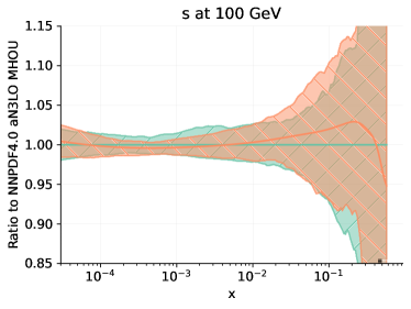
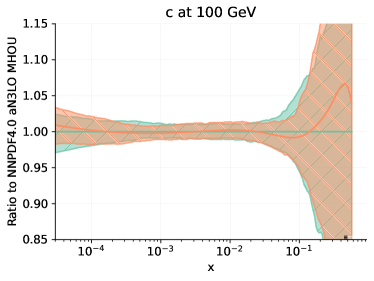
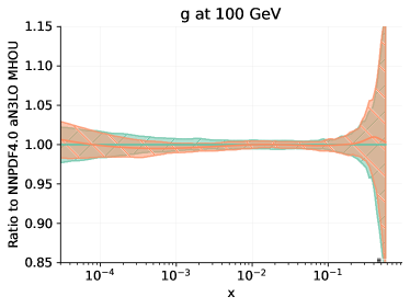
Figure 4.14: Same as Fig. 4.13 for aN³LO PDF sets with MHOUs.

We now discuss two variants in the treatment of aN³LO corrections: a different approximation to perturbative evolution, and a different treatment of hadronic cross-sections.

The aN³LO PDF sets presented in Sect. 4.2 are based on our approximation to the full set of N³LO splitting functions presented in Sect. 2. This approximation was compared in Sect. 2.7 to that recently presented in Refs. [22, 28, 29, 30] (FHMRUVV). In order to fully assess the impact of this different approximation to N³LO perturbative evolution we have repeated the aN³LO PDF determination, without and with MHOUs, but now using the FHMRUVV approximation to N³LO perturbative evolution, with everything else unchanged. PDFs obtained using the FHMRUVV approximation vs our own are compared in Fig. 4.13 without MHOUs and in Fig. 4.14 with MHOUs. PDFs are displayed at $Q=100$ GeV, normalized to the central value of our default result. Differences turn out to be completely negligible, as might have been expected given the good agreement at the level of splitting functions seen in Fig. 2.9.

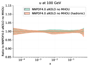
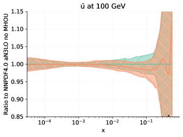
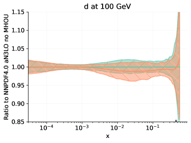
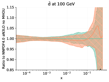
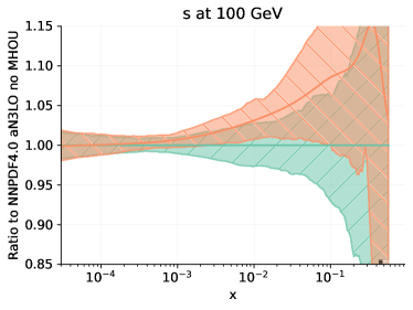
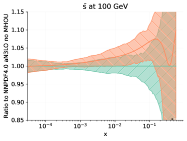
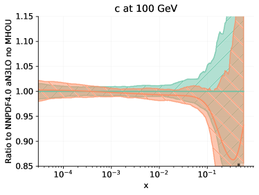
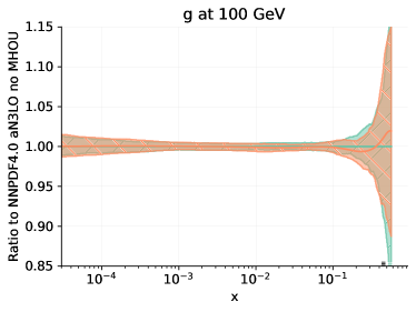
Figure 4.15: Same as Fig. 4.2, now comparing the NNPDF4.0 aN³LO baseline PDF set without MHOUs to a variant obtained with inclusion of N³LO corrections for the hadronic processes of Tab. 3.1.

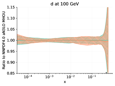
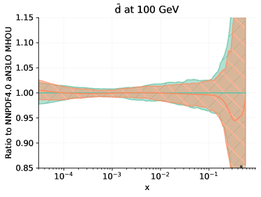
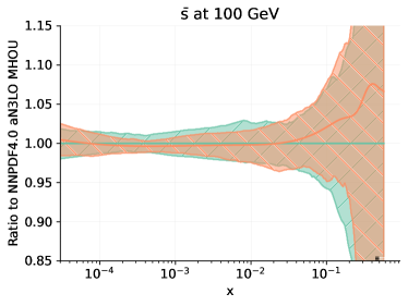
Figure 4.16: Same as Fig. 4.15 for aN³LO PDF sets with MHOUs.

As discussed in Sect. 3.3 N³LO corrections to hadronic hard cross-sections are not included in our default aN³LO PDF determination. We can however assess the impact of the inclusion of all the publicly available corrections for all relevant data in the NNPDF4.0 dataset, listed in Tab. 3.1 and discussed in Sect. 3.3. To this purpose, we have repeated the aN³LO PDF determination, with and without MHOUs, now with N³LO for these datasets included. The ensuing PDFs are compared to the default NNPDF4.0 aN³LO in Fig. 4.15 without MHOUs and in Fig. 4.16 with MHOUs. In both cases, PDFs are displayed at $Q=100$ GeV and are normalized to the central value of the corresponding default NNPDF4.0 aN³LO set. The impact of these N³LO corrections is only (barely) visible in the PDFs without MHOUs, and even in this case it only significantly impacts the strange and antistrange PDFs, for which it leads to an enhancement of 4-5% for $x\sim 0.1$, though well within the PDF uncertainty. Even this small effect is absent in the PDFs with MHOUs. We conclude that at present available N³LO corrections for hadronic processes have no effect on PDF determination.

4.6 Comparison with MSHT20

We compare the NNPDF4.0 aN³LO PDF set to the only other existing aN³LO PDF set, MSHT20 aN³LO [32]. As already discussed in Sect. 2.7, MSHT20 aN³LO PDFs are determined by fitting to the data the nuisance parameters that parametrize the IHOU uncertainty on a prior approximation to splitting functions. It follows that the ensuing central value is partly determined by the data, and the IHOU is entirely data-driven. When comparing NNPDF4.0 and MSHT20 aN³LO PDF sets it should of course be borne in mind that the sets already differ at NNLO due to differences in dataset and methodology. The NNLO MSHT20 and NNPDF4.0 PDF sets were compared in Fig. 21 and the corresponding parton luminosity in Fig. 60 of Ref. [37], while a detailed benchmarking was presented in Ref. [115].

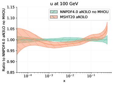
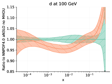
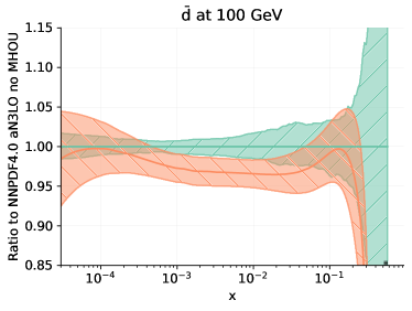
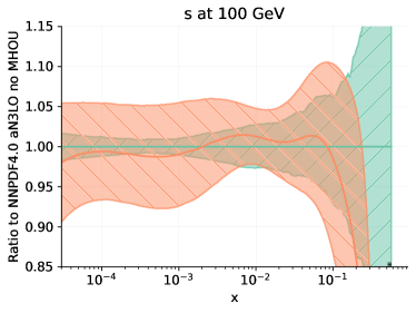
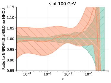
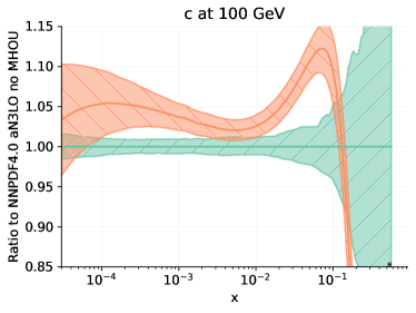
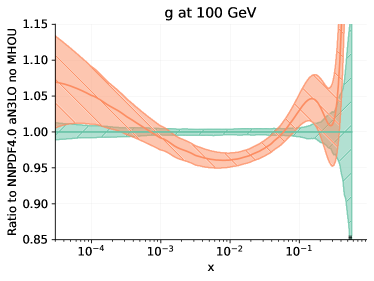
Figure 4.17: Same as Fig. 4.2, now comparing the NNPDF4.0 aN³LO baseline PDF set without MHOUs to the MSHT20 set recommended as baseline in Ref. [32].

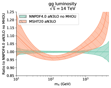
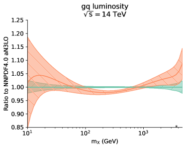
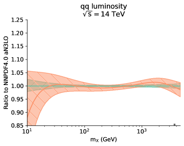
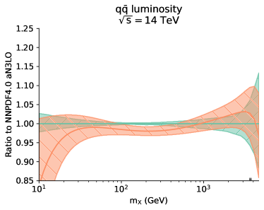
Figure 4.18: Same as Fig. 4.17 for parton luminosities as in Fig. 4.6.

The comparison of the aN³LO sets is presented in Fig. 4.17, where we show the NNPDF4.0 no MHOU set and the MSHT20 set recommended as baseline in Ref. [32] at $Q=100$ GeV, normalized to the NNPDF4.0 central value. All error bands are one sigma uncertainties. The dominant differences between the PDF sets are the same as already observed at NNLO, with the largest difference observed for the charm PDF, which is independently parametrized in NNPDF4.0, but not in MSHT20, where it is determined by perturbative matching conditions. However, the differences, while remaining qualitatively similar, are slightly reduced (by 1-2%) when moving from NNLO to aN³LO. Exceptions are the charm and especially the gluon PDF, which differ more at aN³LO. Specifically, the gluon PDF, while reasonably compatible for $x\lesssim 0.07$ at NNLO, disagrees at aN³LO, with the MSHT20 result suppressed by 3-4% in the region $10^{-3}\lesssim x\lesssim 10^{-1}$, with a PDF uncertainty of 1-2%. This suppression of the MSHT20 gluon can likely be traced to the behaviour of the $P_{gq}$ splitting function seen in Fig. 2.9.

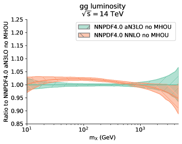
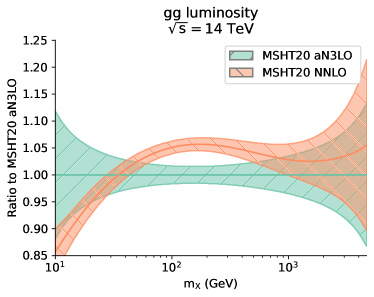
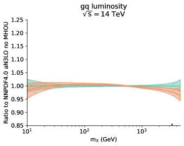
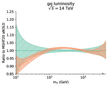
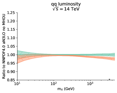
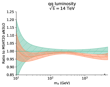
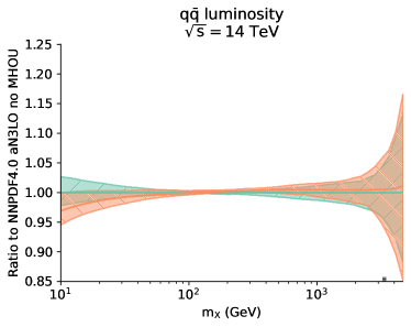
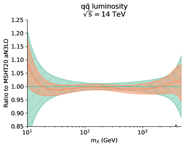
Figure 4.19: Same as Fig. 4.18, now comparing aN³LO and NNLO parton luminosities, separately for the NNPDF4.0 (left) and MSHT20 (right) PDF sets, normalized to the aN³LO result.

Parton luminosities are compared in Fig. 4.18. Again the pattern is similar to that seen at NNLO, but now with a considerable suppression of the gluon-gluon and gluon-quark luminosities in the $M_{X}\sim 100$ GeV region that can be traced to the behaviour of the gluon PDF seen in Fig. 4.17. The quark-quark luminosity remains similar in MSHT20 and NNPDF4.0 both at NNLO and aN³LO. The impact of these effects on the computation of precision LHC cross sections will be addressed in Sect. 5.

In order to understand better the comparative impact of aN³LO corrections, we compare for each set the NNLO and aN³LO luminosities. Results are shown in Fig. 4.19, normalized to the aN³LO result. The qualitative impact of the aN³LO corrections on either set is similar, but with a stronger aN³LO suppression of gluon luminosities for MSHT20. In particular the gluon-gluon luminosity is suppressed for $10^{2}\lesssim m_{X}\lesssim 10^{3}$ GeV by about 3% in NNPDF4.0 and 6% in MSHT20 and the gluon-quark luminosity is suppressed in the same region by about 1% in NNPDF4.0 and 3% in MSHT20. In the case of the gluon-gluon luminosity the differences between NNLO and aN³LO are larger than the respective PDF uncertainties (that do not include MHOUs in either case). As already mentioned in Sect. 2.7, a dedicated benchmark of aN³LO results is ongoing and will be presented in Ref. [84].

5 LHC phenomenology at aN³LO accuracy

We present a first assessment of the implications of aN³LO PDFs for LHC phenomenology, by looking at processes for which N³LO results are publicly available, namely the Drell-Yan and Higgs total inclusive cross-sections. We present predictions at NLO, NNLO, and aN³LO using both NNPDF4.0 and MSHT20 PDFs, consistently matching the perturbative order of the PDF and matrix element. At N³LO we also show results obtained with the currently common approximation of using NNLO PDFs with aN³LO matrix elements.

At each perturbative order, the uncertainty on the cross-section is determined by adding in quadrature the PDF uncertainty to the MHOU on the hard matrix element determined performing 7-point renormalization and factorization scale variation and taking the envelope of the results. This is the procedure that is most commonly used for the estimation of the total uncertainty on hadron collider processes, and we follow it here for ease of comparison with available results. In a more refined treatment, MHOUs on the hard cross section can be included through a theory covariance matrix for the hard cross section itself, like the MHOUs and IHOUs on the PDF. This would then make it possible to keep track of the correlation between these different sources of uncertainty [116, 117, 118]. Here, in order to disentangle the contribution of the MHOU in the processes used for PDF determination from that in the matrix element, we show results with the PDF uncertainty evaluated with both MHOU and no-MHOU PDF sets.

5.1 Inclusive Drell-Yan production

We show results for inclusive charged-current and neutral-current gauge boson production cross-sections followed by their decays into the dilepton final state. Cross-sections are evaluated using the n3loxs code [8] for different ranges in the final-state dilepton invariant mass, $Q=m_{\ell\ell}$ for neutral-current and $Q=m_{\ell\nu}$ for charged-current scattering. Fig. 5.1 displays the inclusive neutral-current Drell-Yan cross-section $pp\to\gamma^{*}/Z\to\ell^{+}\ell^{-}$ and Figs. 5.2-5.3 the charged-current cross-sections $pp\to W^{\pm}\to\ell^{\pm}\nu_{\ell}$. We consider one low-mass bin ($30~{}{\rm GeV}\leq Q\leq 60~{}{\rm GeV}$), the mass peak bin ($60~{}{\rm GeV}\leq Q\leq 120~{}{\rm GeV}$), and two high-mass bins ($120~{}{\rm GeV}\leq Q\leq 300~{}{\rm GeV}$ and $2~{}{\rm TeV}\leq Q\leq 3~{}{\rm TeV}$), relevant for high-mass new physics searches [119]. In all cases, we compare the NLO, NNLO, and aN³LO predictions using NNPDF4.0 and MSHT20 PDFs determinations, with the same perturbative order in matrix element and PDFs, and also the aN³LO result with NNLO PDFs, and then we compare the aN³LO with NNPDF4.0 aN³LO PDFs with and without MHOUs.

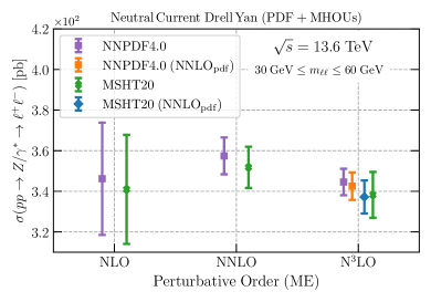
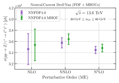
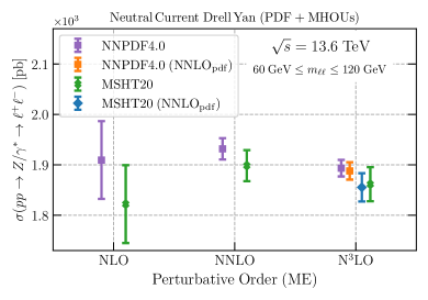
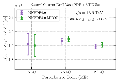
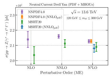
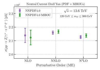
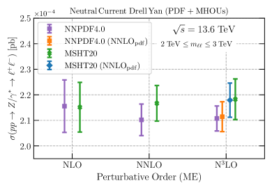
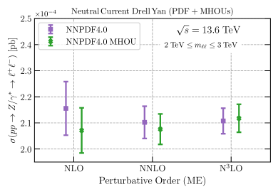
Figure 5.1: The inclusive neutral-current Drell-Yan production cross-section, $pp\to\gamma^{*}/Z\to\ell^{+}\ell^{-}$, for different ranges of the dilepton invariant mass $Q=m_{\ell\ell}$, from low to high invariant masses (top to bottom). Results are shown (left) comparing NLO, NNLO and aN³LO with matched perturbative order in the matrix element and PDF, and also at aN³LO with NNLO PDFs using NNPDF4.0 and MSHT20 PDFs and (right) at aN³LO with PDFs without and with MHOUs.

In general we observe a good perturbative convergence, with predictions at two subsequent orders in agreement within uncertainties, and generally improved convergence upon including MHOUs on the PDF. Predictions based on NNPDF4.0 and MSHT20 are always consistent with each other within uncertainties. From these comparisons we can draw two main conclusions. First, in many cases differences between the NNLO and N³LO predictions tend to be reduced when using consistently the appropriate PDFs at each order, rather than NNLO PDFs with N³LO matrix elements (though in some cases the results are unchanged). For instance, for the two lowest $m_{\ell\ell}$ bins for NC production aN³LO PDFs drive upwards the N³LO prediction, making it closer to the NNLO result. Second, the difference between PDFs with and without MHOUs, while moderate, remains non-negligible even at N³LO, where it starts being comparable to the overall uncertainty, and thus it must be included in precision calculations.

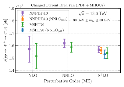
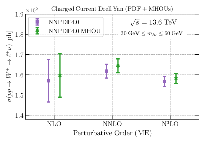
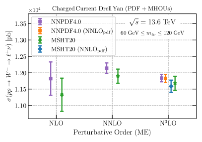
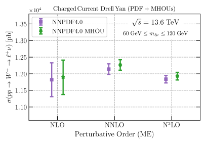
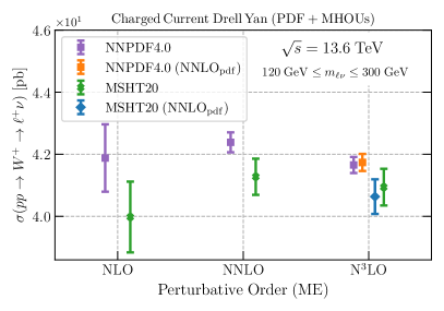
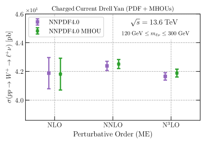
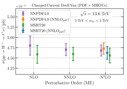
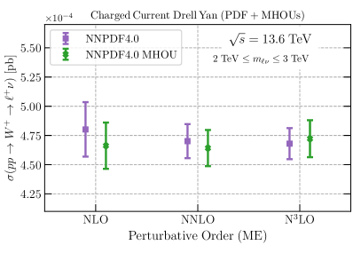
Figure 5.2: Same as Fig. 5.1 for the inclusive charged-current Drell-Yan production cross-section, $pp\to W^{+}\to\ell^{+}\nu_{\ell}$.

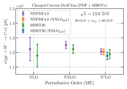
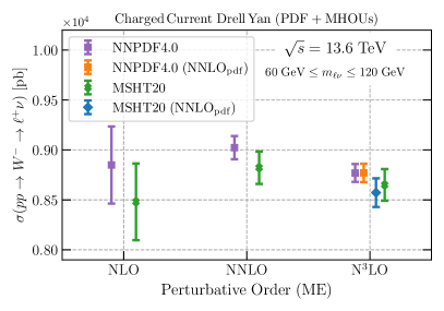
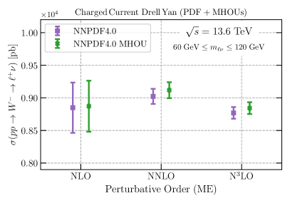
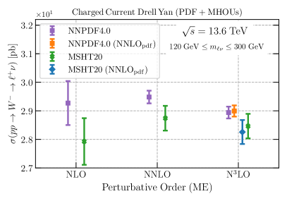
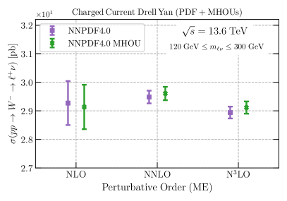
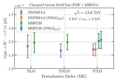
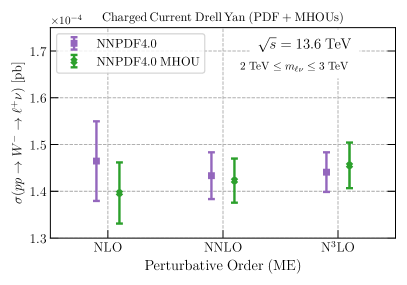
Figure 5.3: Same as Fig. 5.1 for the inclusive charged-current Drell-Yan production cross-section, $pp\to W^{-}\to\ell^{-}\bar{\nu}_{\ell}$.

5.2 Inclusive Higgs production

We now consider Higgs production in gluon fusion, in associated production with vector bosons, and via vector-boson fusion (VBF). Predictions are obtained using the ggHiggs code [120] for gluon fusion, n3loxs for associate production, and proVBFH code [121] for VBF. Results are shown in Fig. 5.4 for gluon-fusion and VBF, and Fig. 5.5 for associate production with $W^{+}$ and $Z$.

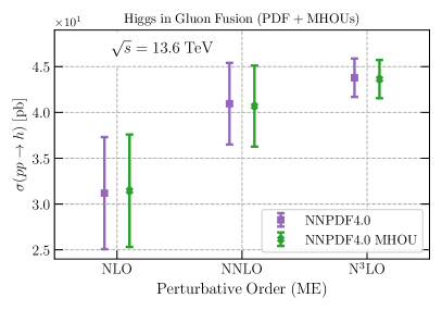
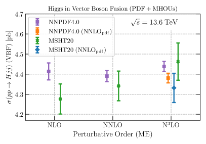
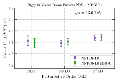
Figure 5.4: Same as Fig. 5.1 for Higgs production in gluon-fusion and via vector-boson fusion.

Here too we observe generally good perturbative convergence, even for gluon fusion, that notoriously has a very slowly converging expansion. Also in this case, there is generally better agreement between NNPDF4.0 and MSHT20 as the perturbative order increases, except for gluon fusion where the agreement is similar at all orders. Indeed, in all cases MSHT20 and NNPDF4.0 results agree within uncertainties at aN³LO, while they do not at NLO for VBF, nor at NLO and NNLO for associated production. The impact of using aN³LO PDFs instead of NNLO PDFs at N³LO for NNPDF4.0 is very moderate for gluon fusion, somewhat more significant for associated production, and more significant for VBF, in which it is comparable to the PDF uncertainty. For MSHT20 instead a significant from using aN³LO instead of NNLO PDFs is also observed for gluon fusion, where suppression of the cross-sections is seen when replacing NNLO with aN³LO PDFs. This follows from the behaviour of the gluon luminosity seen in Fig. 4.19. The impact of MHOUs on the PDFs is generally quite small on the scale of the PDF uncertainty at all perturbative orders, and essentially absent for gluon fusion. For associated production it marginally improves perturbative convergence.

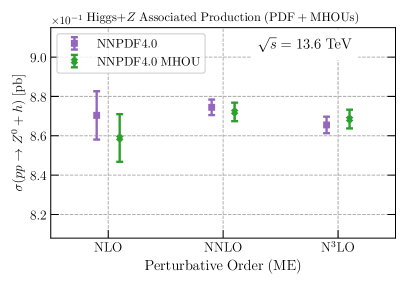
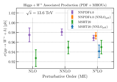
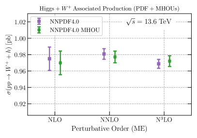
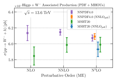
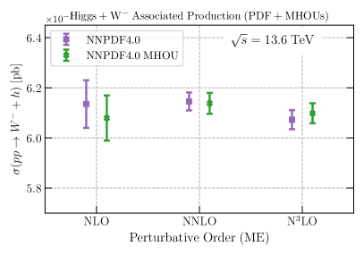
Figure 5.5: Same as Fig. 5.1 for Higgs production in association with $W^{+}$ and $Z$ gauge bosons: from top to bottom, $Zh$, $W^{+}h$, and $W^{-}h$.

6 Summary and outlook

We have presented the first aN³LO PDF sets within the NNPDF framework, by constructing a full set of approximate N³LO splitting functions based on available partial results and known limits, approximate massive DIS coefficient functions, and extending to this order the FONLL general-mass scheme for DIS coefficient functions. We now summarize the new PDF sets that we are releasing, our main conclusions on their features, and our plans for future developments.

The NNPDF4.0 aN³LO PDF sets are available via the LHAPDF6 interface,

http://lhapdf.hepforge.org/  .

Specifically, we provide an aN³LO NNPDF4.0 set

NNPDF40_an3lo_as_01180

that supplements the LO, NLO and NNLO sets of Ref. [37].
We also provide NLO and aN³LO NNPDF4.0MHOU sets

NNPDF40_nlo_as_01180_mhou
NNPDF40_an3lo_as_01180_mhou

that supplement the NNLO NNPDF4.0MHOU PDF set of Ref. [38]. These sets include in the PDF uncertainty the MHOU on the processes used for PDF determination, but in all other respects (including the dataset) follow the default sets to which they can be directly compared.

For both aN³LO sets, we also release the corresponding sets including $\alpha_{s}$ variations,

NNPDF40_an3lo_as_01180_pdfas
NNPDF40_an3lo_as_01180_mhou_pdfas

in which replicas 101 and 102 correspond to fits with $\alpha_{s}(m_{Z})=0.117$ and 0.119 respectively, in order to evaluate the combined PDF+$\alpha_{s}$ uncertainties following the prescription of [122, 123, 115].

All these sets are delivered as ensembles of $N_{\rm rep}=100$ Monte Carlo replicas.
However, we also make available Hessian variants following [124, 125] and denoted

NNPDF40_an3lo_as_01180_hessian
NNPDF40_an3lo_as_01180_mhou_hessian
NNPDF40_an3lo_as_01180_pdfas_hessian
NNPDF40_an3lo_as_01180_mhou_pdfas_hessian

each set comprising $N_{\rm eig}=100$ eigenvectors.

All these sets are also available on the NNPDF Collaboration website,

https://nnpdf.mi.infn.it/nnpdf4-0-n3lo/  .

where we also give the PDF sets discussed in Sect. 4.5 based on variant treatments of the aN³LO corrections. In addition to the LHAPDF grids themselves, all the results obtained in this work are reproducible by means of the open-source NNPDF code [39] and the related suite of theory tools.

We have provided a first assessment of these PDF sets by comparing them to their NLO and NNLO counterparts with and without MHOUs. Our main conclusions are the following

• For all PDFs good perturbative convergence is observed, with differences decreasing as the perturbative order increases, and the aN³LO result always compatible with the NNLO within uncertainties.

• For quark PDFs the difference between NNLO and aN³LO results is extremely small, suggesting that with current data and methodology the effect of yet higher orders is negligible.

• For the gluon PDF a more significant shift is observed between NNLO and N³LO, thus making the inclusion of N³LO important for precision phenomenology.

• The inclusion of MHOUs improves perturbative convergence, mostly by shifting central values at each order towards the higher-order result, by an amount that decreases with increasing perturbative order.

• Upon inclusion of MHOUs the fit quality becomes all but independent of perturbative order, and PDF uncertainties generally decrease (or remain unchanged) due to the improved data compatibility.

• The effect of MHOUs at N³LO is very small for quarks but not negligible for the gluon PDF.

• Evidence for intrinsic charm is somewhat increased already at NNLO by the inclusion of MHOUs, and somewhat increased again when going from NNLO to N³LO.

• The impact of N³LO corrections on the total cross-section for Higgs in gluon fusion is very small on the scale of the PDF uncertainty.

All in all, these results underline the importance of the inclusion of N³LO corrections and MHOUs for precision phenomenology at sub-percent accuracy.

Future NNPDF releases will include by default MHOUs, will be at all orders up to aN³LO, and will include a photon PDF. Specifically, we aim to extend to aN³LO with MHOUs our recent construction of NNPDF4.0QED PDFs [109]. Indeed, aN³LO PDFs including a photon PDF (such as those recently released by MSHT20 [126]) will be a necessary ingredient for theory predictions based on state-of-the art QCD and electroweak (EW) corrections. In fact, we are working towards the consistent inclusion of combined QCD$\times$EW corrections also in the theory predictions used for PDF determination.

Another important line of future development involves the all-order resummation of potentially large perturbative contributions in the large $x$ and small $x$ regions [127, 69]. This will involve matching resummed and fixed-order cross-sections and (at small $x$) perturbative evolution in the new streamlined NNPDF theory pipeline. Such resummed PDFs will be instrumental for precision phenomenology: specifically at small $x$, forward neutrino production at the LHC and scattering processes for high-energy astroparticle physics, and at large $x$, searches for new physics in high-mass final states at the LHC and future hadron colliders.

 

Acknowledgments

We thank James McGowan, Thomas Cridge, Lucian Harland-Lang, and Robert Thorne for discussions on MSHT20 PDFs. We are grateful to Sven Moch and Joshua Davies for discussion and for communications concerning their N³LO results..

R.D.B, L.D.D, and R.S. are supported by the U.K. Science and Technology Facility Council (STFC) consolidated grants ST/T000600/1 and ST/X000494/1. F.H. is supported by the Academy of Finland project 358090 and is funded as a part of the Center of Excellence in Quark Matter of the Academy of Finland, project 346326. E.R.N. is supported by the Italian Ministry of University and Research (MUR) through the “Rita Levi-Montalcini” Program. M.U. and Z.K. are supported by the European Research Council under the European Union’s Horizon 2020 research and innovation Programme (grant agreement n.950246), and partially by the STFC consolidated grant ST/T000694/1 and ST/X000664/1. J.R. is partially supported by NWO, the Dutch Research Council. C.S. is supported by the German Research Foundation (DFG) under reference number DE 623/6-2.

Appendix A Explicit expressions of anomalous dimensions

We provide here explicit expressions for the $\gamma_{{\rm ns}\,\pm,\,N\to\infty}^{(3)}(N)$ and $\gamma_{{\rm ns}\,\pm,\,N\to 0}^{(3)}(N)$ anomalous dimension discussed in Sect. 2.3 and the $\gamma_{{\rm ns}\,\pm,\,N\to\infty}^{(3)}(N)$, $\gamma_{{\rm ns}\,\pm,\,N\to 0}^{(3)}(N)$ and $\gamma_{{\rm ns}\,\pm,\,N\to 1}^{(3)}(N)$ discussed in Sect. 2.4.

$\gamma_{{\rm ns},\pm}^{(3)}(N)$:

$$\begin{split}\gamma_{{\rm ns},\pm,N\to 0}^{(3)}(N)&=-\frac{252.84}{N^{7}}+\frac{1580.25-126.42n_{f}}{N^{6}}\\ &+\frac{-5806.8+752.198n_{f}-18.963n_{f}^{2}}{N^{5}}\\ &+\frac{14899.9-2253.11n_{f}+99.1605n_{f}^{2}-0.790123n_{f}^{3}}{N^{4}}\\ &+\frac{-28546.4+5247.18n_{f}-226.441n_{f}^{2}+2.89712n_{f}^{3}}{N^{3}}\\ &+\frac{50759.7-8769.15n_{f}+395.605n_{f}^{2}-3.16049n_{f}^{3}}{N^{2}}\end{split}$$ (A.1)

$$\begin{split}\gamma_{{\rm ns},\pm N\to\infty}^{(3)}(N)&=\left(+20702.4-5171.92n_{f}+195.577n_{f}^{2}+3.27234n_{f}^{3}\right)S_{1}(N)\\ &-23393.8+5550.04n_{f}-193.855n_{f}^{2}-3.01498n_{f}^{3}\\ &+\left(16950.9-2741.83n_{f}+26.6886n_{f}^{2}\right)\frac{S_{1}(N)}{N}\\ &+\frac{+11126.6-3248.4n_{f}+180.432n_{f}^{2}+0.526749n_{f}^{3}}{N}\end{split}$$ (A.2)

$\gamma_{gg}^{(3)}(N)$:

$$\begin{split}\gamma_{gg,N\to 0}^{(3)}(N)&=\frac{-103680+20005.9n_{f}-568.889n_{f}^{2}}{N^{7}}\\ &+\frac{-17280-19449.7n_{f}+1725.63n_{f}^{2}}{N^{6}}\\ &+\frac{-627979+80274.1n_{f}-2196.54n_{f}^{2}+4.74074n_{f}^{3}}{N^{5}}\end{split}$$ (A.3)

$$\gamma_{gg,N\to 1}^{(3)}(N)=-\frac{49851.7}{(N-1)^{4}}+\frac{213824+1992.77n_{f}}{(N-1)^{3}}$$ (A.4)

$$\begin{split}\gamma_{gg,N\to\infty}^{(3)}(N)&=\left(+40880.3-11714.2n_{f}+440.049n_{f}^{2}+7.36278n_{f}^{3}\right)S_{1}(N)\\ &-68587.9+18144n_{f}-423.811n_{f}^{2}-0.906722n_{f}^{3}\\ &-\left(-85814.1+13880.5n_{f}-135.111n_{f}^{2}\right)\frac{S_{1}(N)}{N}\\ &+\frac{-54482.8+4341.13n_{f}+21.3333n_{f}^{2}}{N}\end{split}$$ (A.5)

$\gamma_{gq}^{(3)}(N)$:

$$\begin{split}\gamma_{gq,N\to 0}^{(3)}(N)&=\frac{-37609.9+5309.63n_{f}}{N^{7}}\\ &+\frac{-35065.7+221.235n_{f}}{N^{6}}\\ &+\frac{-175455+9092.91n_{f}+778.535n_{f}^{2}}{N^{5}}\end{split}$$ (A.6)

$$\gamma_{gq,N\to 1}^{(3)}(N)=-\frac{22156.3}{(N-1)^{4}}+\frac{95032.9+885.674n_{f}}{(N-1)^{3}}$$ (A.7)

$$\begin{split}\gamma_{gq,N\to\infty}^{(3)}(N)&=\left(-13.4431+0.548697n_{f}\right)L_{5,0}(N)\\ &+\left(-375.398+34.4947n_{f}-0.877915n_{f}^{2}\right)L_{4,0}(N)\end{split}$$ (A.8)

$\gamma_{qg}^{(3)}(N)$:

$$\begin{split}\gamma_{qg,N\to 0}^{(3)}(N)&=\frac{14103.7n_{f}-1991.11n_{f}^{2}}{N^{7}}\\ &+\frac{2588.84n_{f}+2069.33n_{f}^{2}}{N^{6}}\\ &+\frac{68802.3n_{f}-7229.38n_{f}^{2}-99.1605n_{f}^{3}}{N^{5}}\end{split}$$ (A.9)

$$\gamma_{qg,N\to 1}^{(3)}(N)=-\frac{7871.52n_{f}}{(N-1)^{3}}$$ (A.10)

$$\begin{split}\gamma_{qg,N\to\infty}^{(3)}(N)&=\left(-1.85185n_{f}+0.411523n_{f}^{2}\right)L_{5,0}(N)\\ &+\left(-35.6878n_{f}+3.51166n_{f}^{2}+0.0823045n_{f}^{3}\right)L_{4,0}(N)\\ &+\left(-2.88066n_{f}-0.823045n_{f}^{2}\right)L_{5,1}(N)\\ &+\left(+40.5114n_{f}-5.54184n_{f}^{2}-0.164609n_{f}^{3}\right)L_{4,1}(N)\end{split}$$ (A.11)

$\gamma_{qq,{\rm ps}}^{(3)}(N)$:

$$\begin{split}\gamma_{qq,{\rm ps},N\to 0}^{(3)}(N)&=\frac{5404.44n_{f}-568.889n_{f}^{2}}{N^{7}}\\ &+\frac{3425.98n_{f}+455.111n_{f}^{2}}{N^{6}}\\ &+\frac{20515.2n_{f}-1856.79n_{f}^{2}+4.74074n_{f}^{3}}{N^{5}}\end{split}$$ (A.12)

$$\gamma_{qq,{\rm ps},N\to 1}^{(3)}(N)=-\frac{3498.45n_{f}}{(N-1)^{3}},$$ (A.13)

$$\begin{split}\gamma_{qq,{\rm ps},N\to\infty}^{(3)}(N)&=\left(+56.4609n_{f}-3.6214n_{f}^{2}\right)L_{4,1}(N)\\ &+\left(+247.551n_{f}-40.5597n_{f}^{2}+1.58025n_{f}^{3}\right)L_{3,1}(N)\\ &+13.1687n_{f}L_{4,2}(N)\\ &+\left(+199.111n_{f}-13.6955n_{f}^{2}\right)L_{3,2}(N).\end{split}$$ (A.14)

The functions $L_{k,j}(N)$ are defined as the Mellin transform of $(1-x)^{j}\ln^{k}(1-x)$:

$$L_{k,0}(N) =\mathcal{M}\left[\ln^{k}(1-x)\right](N)=(-1)^{k}k!\frac{S_{1_{k},\dots,1_{1}}(N)}{N}$$ (A.15)

$$L_{k,1}(N) =\mathcal{M}\left[(1-x)\ln^{k}(1-x)\right]=L_{k,0}(N)-L_{k,0}(N+1)$$ (A.16)

$$L_{k,2}(N) =\mathcal{M}\left[(1-x)^{2}\ln^{k}(1-x)\right]=L_{k,0}(N)-2L_{k,0}(N+1)+L_{k,0}(N+2)$$ (A.17)

with the multi-index harmonics of weight-$k$ defined recursively as:

$$S_{1_{k},\dots,1_{1}}(N)=\sum_{j=1}^{N}\frac{S_{1_{k-1},\dots,1_{1}}(j)}{j}\ .$$ (A.18)

References

- [1] J. A. M. Vermaseren, A. Vogt, and S. Moch, The third-order QCD corrections to deep-inelastic scattering by photon exchange, Nucl. Phys. B724 (2005) 3, [hep-ph/0504242].
- [2] S. Moch, J. A. M. Vermaseren, and A. Vogt, The longitudinal structure function at the third order, Phys. Lett. B606 (2005) 123, [hep-ph/0411112].
- [3] S. Moch, M. Rogal, and A. Vogt, Differences between charged-current coefficient functions, Nucl. Phys. B790 (2008) 317–335, [arXiv:0708.3731].
- [4] S. Moch, J. A. M. Vermaseren, and A. Vogt, Third-order QCD corrections to the charged-current structure function F(3), Nucl. Phys. B 813 (2009) 220–258, [arXiv:0812.4168].
- [5] C. Anastasiou, C. Duhr, F. Dulat, F. Herzog, and B. Mistlberger, Higgs Boson Gluon-Fusion Production in QCD at Three Loops, Phys. Rev. Lett. 114 (2015), no. 21 212001, [arXiv:1503.06056].
- [6] B. Mistlberger, Higgs boson production at hadron colliders at N3LO in QCD, JHEP 05 (2018) 028, [arXiv:1802.00833].
- [7] C. Duhr, F. Dulat, and B. Mistlberger, Higgs Boson Production in Bottom-Quark Fusion to Third Order in the Strong Coupling, Phys. Rev. Lett. 125 (2020), no. 5 051804, [arXiv:1904.09990].
- [8] J. Baglio, C. Duhr, B. Mistlberger, and R. Szafron, Inclusive production cross sections at N3LO, JHEP 12 (2022) 066, [arXiv:2209.06138].
- [9] F. A. Dreyer and A. Karlberg, Vector-Boson Fusion Higgs Production at Three Loops in QCD, Phys. Rev. Lett. 117 (2016), no. 7 072001, [arXiv:1606.00840].
- [10] L.-B. Chen, H. T. Li, H.-S. Shao, and J. Wang, Higgs boson pair production via gluon fusion at N3LO in QCD, Phys. Lett. B 803 (2020) 135292, [arXiv:1909.06808].
- [11] C. Duhr, F. Dulat, and B. Mistlberger, Charged current Drell-Yan production at N3LO, JHEP 11 (2020) 143, [arXiv:2007.13313].
- [12] C. Duhr and B. Mistlberger, Lepton-pair production at hadron colliders at N3LO in QCD, JHEP 03 (2022) 116, [arXiv:2111.10379].
- [13] F. Dulat, B. Mistlberger, and A. Pelloni, Differential Higgs production at N3LO beyond threshold, JHEP 01 (2018) 145, [arXiv:1710.03016].
- [14] F. Dulat, B. Mistlberger, and A. Pelloni, Precision predictions at N3LO for the Higgs boson rapidity distribution at the LHC, Phys. Rev. D 99 (2019), no. 3 034004, [arXiv:1810.09462].
- [15] X. Chen, T. Gehrmann, E. W. N. Glover, A. Huss, B. Mistlberger, and A. Pelloni, Fully Differential Higgs Boson Production to Third Order in QCD, Phys. Rev. Lett. 127 (2021), no. 7 072002, [arXiv:2102.07607].
- [16] G. Billis, B. Dehnadi, M. A. Ebert, J. K. L. Michel, and F. J. Tackmann, Higgs pT Spectrum and Total Cross Section with Fiducial Cuts at Third Resummed and Fixed Order in QCD, Phys. Rev. Lett. 127 (2021), no. 7 072001, [arXiv:2102.08039].
- [17] S. Camarda, L. Cieri, and G. Ferrera, Drell–Yan lepton-pair production: qT resummation at N3LL accuracy and fiducial cross sections at N3LO, Phys. Rev. D 104 (2021), no. 11 L111503, [arXiv:2103.04974].
- [18] X. Chen, T. Gehrmann, N. Glover, A. Huss, T.-Z. Yang, and H. X. Zhu, Dilepton Rapidity Distribution in Drell-Yan Production to Third Order in QCD, Phys. Rev. Lett. 128 (2022), no. 5 052001, [arXiv:2107.09085].
- [19] X. Chen, T. Gehrmann, N. Glover, A. Huss, T.-Z. Yang, and H. X. Zhu, Transverse mass distribution and charge asymmetry in W boson production to third order in QCD, Phys. Lett. B 840 (2023) 137876, [arXiv:2205.11426].
- [20] F. Caola, W. Chen, C. Duhr, X. Liu, B. Mistlberger, F. Petriello, G. Vita, and S. Weinzierl, The Path forward to N3LO, in Snowmass 2021, 3, 2022. arXiv:2203.06730.
- [21] J. Davies, A. Vogt, B. Ruijl, T. Ueda, and J. A. M. Vermaseren, Large-nf contributions to the four-loop splitting functions in QCD, Nucl. Phys. B 915 (2017) 335–362, [arXiv:1610.07477].
- [22] S. Moch, B. Ruijl, T. Ueda, J. A. M. Vermaseren, and A. Vogt, Four-Loop Non-Singlet Splitting Functions in the Planar Limit and Beyond, JHEP 10 (2017) 041, [arXiv:1707.08315].
- [23] J. Davies, C. H. Kom, S. Moch, and A. Vogt, Resummation of small-x double logarithms in QCD: inclusive deep-inelastic scattering, JHEP 08 (2022) 135, [arXiv:2202.10362].
- [24] J. M. Henn, G. P. Korchemsky, and B. Mistlberger, The full four-loop cusp anomalous dimension in super Yang-Mills and QCD, JHEP 04 (2020) 018, [arXiv:1911.10174].
- [25] C. Duhr, B. Mistlberger, and G. Vita, Soft integrals and soft anomalous dimensions at N3LO and beyond, JHEP 09 (2022) 155, [arXiv:2205.04493].
- [26] S. Moch, B. Ruijl, T. Ueda, J. A. M. Vermaseren, and A. Vogt, Low moments of the four-loop splitting functions in QCD, Phys. Lett. B 825 (2022) 136853, [arXiv:2111.15561].
- [27] G. Soar, S. Moch, J. A. M. Vermaseren, and A. Vogt, On Higgs-exchange DIS, physical evolution kernels and fourth-order splitting functions at large x, Nucl. Phys. B 832 (2010) 152–227, [arXiv:0912.0369].
- [28] G. Falcioni, F. Herzog, S. Moch, and A. Vogt, Four-loop splitting functions in QCD – The quark-quark case, Phys. Lett. B 842 (2023) 137944, [arXiv:2302.07593].
- [29] G. Falcioni, F. Herzog, S. Moch, and A. Vogt, Four-loop splitting functions in QCD – The gluon-to-quark case, Phys. Lett. B 846 (2023) 138215, [arXiv:2307.04158].
- [30] S. Moch, B. Ruijl, T. Ueda, J. Vermaseren, and A. Vogt, Additional moments and x-space approximations of four-loop splitting functions in QCD, Phys. Lett. B 849 (2024) 138468, [arXiv:2310.05744].
- [31] G. Falcioni, F. Herzog, S. Moch, J. Vermaseren, and A. Vogt, The double fermionic contribution to the four-loop quark-to-gluon splitting function, Phys. Lett. B 848 (2024) 138351, [arXiv:2310.01245].
- [32] J. McGowan, T. Cridge, L. A. Harland-Lang, and R. S. Thorne, Approximate N3LO parton distribution functions with theoretical uncertainties: MSHT20aN3LO PDFs, Eur. Phys. J. C 83 (2023), no. 3 185, [arXiv:2207.04739]. [Erratum: Eur.Phys.J.C 83, 302 (2023)].
- [33] W. L. van Neerven and A. Vogt, Improved approximations for the three loop splitting functions in QCD, Phys. Lett. B 490 (2000) 111–118, [hep-ph/0007362].
- [34] NNPDF Collaboration, R. D. Ball, E. R. Nocera, and R. L. Pearson, Nuclear Uncertainties in the Determination of Proton PDFs, Eur. Phys. J. C79 (2019), no. 3 282, [arXiv:1812.09074].
- [35] NNPDF Collaboration, R. Abdul Khalek et al., A first determination of parton distributions with theoretical uncertainties, Eur. Phys. J. C (2019) 79:838, [arXiv:1905.04311].
- [36] NNPDF Collaboration, R. Abdul Khalek et al., Parton Distributions with Theory Uncertainties: General Formalism and First Phenomenological Studies, Eur. Phys. J. C 79 (2019), no. 11 931, [arXiv:1906.10698].
- [37] NNPDF Collaboration, R. D. Ball et al., The path to proton structure at 1% accuracy, Eur. Phys. J. C 82 (2022), no. 5 428, [arXiv:2109.02653].
- [38] NNPDF Collaboration, R. D. Ball et al., Determination of the theory uncertainties from missing higher orders on NNLO parton distributions with percent accuracy, arXiv:2401.10319.
- [39] NNPDF Collaboration, R. D. Ball et al., An open-source machine learning framework for global analyses of parton distributions, Eur. Phys. J. C 81 (2021), no. 10 958, [arXiv:2109.02671].
- [40] A. Candido, F. Hekhorn, and G. Magni, EKO: evolution kernel operators, Eur. Phys. J. C 82 (2022), no. 10 976, [arXiv:2202.02338].
- [41] A. Candido, F. Hekhorn, G. Magni, T. R. Rabemananjara, and R. Stegeman, Yadism: Yet Another Deep-Inelastic Scattering Module, arXiv:2401.15187.
- [42] S. Forte, E. Laenen, P. Nason, and J. Rojo, Heavy quarks in deep-inelastic scattering, Nucl. Phys. B834 (2010) 116–162, [arXiv:1001.2312].
- [43] R. D. Ball, M. Bonvini, and L. Rottoli, Charm in Deep-Inelastic Scattering, JHEP 11 (2015) 122, [arXiv:1510.02491].
- [44] R. D. Ball, V. Bertone, M. Bonvini, S. Forte, P. Groth Merrild, J. Rojo, and L. Rottoli, Intrinsic charm in a matched general-mass scheme, Phys. Lett. B754 (2016) 49–58, [arXiv:1510.00009].
- [45] A. Vogt, Efficient evolution of unpolarized and polarized parton distributions with QCD-PEGASUS, Comput. Phys. Commun. 170 (2005) 65–92, [hep-ph/0408244].
- [46] T. Gehrmann, A. von Manteuffel, V. Sotnikov, and T.-Z. Yang, The contribution to the non-singlet splitting function at four-loop order, Phys. Lett. B 849 (2024) 138427, [arXiv:2310.12240].
- [47] S. Albino and R. D. Ball, Soft resummation of quark anomalous dimensions and coefficient functions in MS-bar factorization, Phys. Lett. B 513 (2001) 93–102, [hep-ph/0011133].
- [48] R. D. Ball, M. Bonvini, S. Forte, S. Marzani, and G. Ridolfi, Higgs production in gluon fusion beyond NNLO, Nucl.Phys. B874 (2013) 746, [arXiv:1303.3590].
- [49] T. Gehrmann, A. von Manteuffel, V. Sotnikov, and T.-Z. Yang, Complete contributions to four-loop pure-singlet splitting functions, JHEP 01 (2024) 029, [arXiv:2308.07958].
- [50] V. S. Fadin, E. A. Kuraev, and L. N. Lipatov, On the Pomeranchuk Singularity in Asymptotically Free Theories, Phys. Lett. B 60 (1975) 50–52.
- [51] E. A. Kuraev, L. N. Lipatov, and V. S. Fadin, Multi - Reggeon Processes in the Yang-Mills Theory, Sov. Phys. JETP 44 (1976) 443–450.
- [52] L. N. Lipatov, Reggeization of the Vector Meson and the Vacuum Singularity in Nonabelian Gauge Theories, Sov. J. Nucl. Phys. 23 (1976) 338–345.
- [53] E. A. Kuraev, L. N. Lipatov, and V. S. Fadin, The Pomeranchuk Singularity in Nonabelian Gauge Theories, Sov. Phys. JETP 45 (1977) 199–204.
- [54] I. I. Balitsky and L. N. Lipatov, The Pomeranchuk Singularity in Quantum Chromodynamics, Sov. J. Nucl. Phys. 28 (1978) 822–829.
- [55] V. S. Fadin and L. N. Lipatov, Next-to-leading corrections to the BFKL equation from the gluon and quark production, Nucl. Phys. B 477 (1996) 767–808, [hep-ph/9602287].
- [56] V. S. Fadin, R. Fiore, A. Flachi, and M. I. Kotsky, Quark - anti-quark contribution to the BFKL kernel, Phys. Lett. B 422 (1998) 287–293, [hep-ph/9711427].
- [57] V. S. Fadin, M. I. Kotsky, and L. N. Lipatov, One-loop correction to the BFKL kernel from two gluon production, Phys. Lett. B 415 (1997) 97–103.
- [58] G. Camici and M. Ciafaloni, Irreducible part of the next-to-leading BFKL kernel, Phys. Lett. B 412 (1997) 396–406, [hep-ph/9707390]. [Erratum: Phys.Lett.B 417, 390 (1998)].
- [59] V. S. Fadin and L. N. Lipatov, BFKL pomeron in the next-to-leading approximation, Phys. Lett. B 429 (1998) 127–134, [hep-ph/9802290].
- [60] T. Jaroszewicz, Gluonic Regge Singularities and Anomalous Dimensions in QCD, Phys. Lett. B 116 (1982) 291–294.
- [61] R. D. Ball and S. Forte, Summation of leading logarithms at small x, Phys. Lett. B 351 (1995) 313–324, [hep-ph/9501231].
- [62] R. D. Ball and S. Forte, The Small x behavior of Altarelli-Parisi splitting functions, Phys. Lett. B 465 (1999) 271–281, [hep-ph/9906222].
- [63] M. Bonvini and S. Marzani, Four-loop splitting functions at small , JHEP 06 (2018) 145, [arXiv:1805.06460].
- [64] S. Catani and F. Hautmann, High-energy factorization and small x deep inelastic scattering beyond leading order, Nucl. Phys. B 427 (1994) 475–524, [hep-ph/9405388].
- [65] A. Vogt, S. Moch, and J. A. M. Vermaseren, The Three-loop splitting functions in QCD: The Singlet case, Nucl. Phys. B691 (2004) 129–181, [hep-ph/0404111].
- [66] Y. L. Dokshitzer, G. Marchesini, and G. P. Salam, Revisiting parton evolution and the large-x limit, Phys. Lett. B 634 (2006) 504–507, [hep-ph/0511302].
- [67] A. A. Almasy, G. Soar, and A. Vogt, Generalized double-logarithmic large-x resummation in inclusive deep-inelastic scattering, JHEP 03 (2011) 030, [arXiv:1012.3352].
- [68] G. Altarelli, R. D. Ball, and S. Forte, Small x Resummation with Quarks: Deep-Inelastic Scattering, Nucl. Phys. B799 (2008) 199–240, [arXiv:0802.0032].
- [69] R. D. Ball, V. Bertone, M. Bonvini, S. Marzani, J. Rojo, and L. Rottoli, Parton distributions with small-x resummation: evidence for BFKL dynamics in HERA data, Eur. Phys. J. C78 (2018), no. 4 321, [arXiv:1710.05935].
- [70] A. Barontini, A. Candido, J. M. Cruz-Martinez, F. Hekhorn, and C. Schwan, Pineline: Industrialization of high-energy theory predictions, Comput. Phys. Commun. 297 (2024) 109061, [arXiv:2302.12124].
- [71] I. Bierenbaum, J. Blümlein, and S. Klein, Mellin Moments of the Heavy Flavor Contributions to unpolarized Deep-Inelastic Scattering at and Anomalous Dimensions, Nucl. Phys. B 820 (2009) 417–482, [arXiv:0904.3563].
- [72] I. Bierenbaum, J. Blumlein, S. Klein, and C. Schneider, Two-Loop Massive Operator Matrix Elements for Unpolarized Heavy Flavor Production to O(epsilon), Nucl. Phys. B 803 (2008) 1–41, [arXiv:0803.0273].
- [73] I. Bierenbaum, J. Blümlein, and S. Klein, The Gluonic Operator Matrix Elements at for DIS Heavy Flavor Production, Phys. Lett. B 672 (2009) 401–406, [arXiv:0901.0669].
- [74] J. Ablinger, J. Blümlein, S. Klein, C. Schneider, and F. Wissbrock, The Massive Operator Matrix Elements of for the Structure Function and Transversity, Nucl. Phys. B 844 (2011) 26–54, [arXiv:1008.3347].
- [75] J. Ablinger, A. Behring, J. Blümlein, A. De Freitas, A. Hasselhuhn, A. von Manteuffel, M. Round, C. Schneider, and F. Wißbrock, The 3-Loop Non-Singlet Heavy Flavor Contributions and Anomalous Dimensions for the Structure Function and Transversity, Nucl. Phys. B 886 (2014) 733–823, [arXiv:1406.4654].
- [76] J. Ablinger, J. Blümlein, A. De Freitas, A. Hasselhuhn, A. von Manteuffel, M. Round, and C. Schneider, The Contributions to the Gluonic Operator Matrix Element, Nucl. Phys. B 885 (2014) 280–317, [arXiv:1405.4259].
- [77] A. Behring, I. Bierenbaum, J. Blümlein, A. De Freitas, S. Klein, and F. Wißbrock, The logarithmic contributions to the asymptotic massive Wilson coefficients and operator matrix elements in deeply inelastic scattering, Eur. Phys. J. C 74 (2014), no. 9 3033, [arXiv:1403.6356].
- [78] J. Blümlein, J. Ablinger, A. Behring, A. De Freitas, A. von Manteuffel, C. Schneider, and C. Schneider, Heavy Flavor Wilson Coefficients in Deep-Inelastic Scattering: Recent Results, PoS QCDEV2017 (2017) 031, [arXiv:1711.07957].
- [79] J. Ablinger, J. Blümlein, A. De Freitas, A. Hasselhuhn, A. von Manteuffel, M. Round, C. Schneider, and F. Wißbrock, The transition matrix element of the variable flavor number scheme at , Nuclear Physics B 882 (May, 2014) 263–288.
- [80] J. Ablinger, A. Behring, J. Blümlein, A. De Freitas, A. von Manteuffel, and C. Schneider, The 3-loop pure singlet heavy flavor contributions to the structure function f2(x,q2) and the anomalous dimension, Nuclear Physics B 890 (Jan, 2015) 48–151.
- [81] J. Ablinger, A. Behring, J. Blümlein, A. De Freitas, A. Goedicke, A. von Manteuffel, C. Schneider, and K. Schönwald, The unpolarized and polarized single-mass three-loop heavy flavor operator matrix elements Agg,Q and Agg,Q, JHEP 12 (2022) 134, [arXiv:2211.05462].
- [82] J. Ablinger, A. Behring, J. Blümlein, A. De Freitas, A. von Manteuffel, C. Schneider, and K. Schönwald, The first–order factorizable contributions to the three–loop massive operator matrix elements AQg(3) and AQg(3), Nucl. Phys. B 999 (2024) 116427, [arXiv:2311.00644].
- [83] H. Kawamura, N. A. Lo Presti, S. Moch, and A. Vogt, On the next-to-next-to-leading order QCD corrections to heavy-quark production in deep-inelastic scattering, Nucl. Phys. B 864 (2012) 399–468, [arXiv:1205.5727].
- [84] T. Cridge et al., Approximate N3LO splitting functions benchmarking, in preparation (2024).
- [85] J. Davies, A. Vogt, S. Moch, and J. A. M. Vermaseren, Non-singlet coefficient functions for charged-current deep-inelastic scattering to the third order in QCD, PoS DIS2016 (2016) 059, [arXiv:1606.08907].
- [86] J. Blümlein, P. Marquard, C. Schneider, and K. Schönwald, The massless three-loop Wilson coefficients for the deep-inelastic structure functions F2, FL, xF3 and g1, JHEP 11 (2022) 156, [arXiv:2208.14325].
- [87] N. Laurenti, Construction of a next-to-next-to-next-to-leading order approximation for heavy flavour production in deep inelastic scattering with quark masses, Master’s thesis, Rome Sapienza U., 2021. arXiv:2401.12139.
- [88] A. Barontini, M. Bonvini, and N. Laurenti, Implementation of DIS at N3LO for PDF determinations, in preparation (2024).
- [89] J. C. Collins, F. Wilczek, and A. Zee, Low-Energy Manifestations of Heavy Particles: Application to the Neutral Current, Phys. Rev. D 18 (1978) 242.
- [90] M. Buza, Y. Matiounine, J. Smith, and W. L. van Neerven, Charm electroproduction viewed in the variable flavor number scheme versus fixed order perturbation theory, Eur. Phys. J. C 1 (1998) 301–320, [hep-ph/9612398].
- [91] E. Laenen, S. Riemersma, J. Smith, and W. L. van Neerven, Complete O (alpha-s) corrections to heavy flavor structure functions in electroproduction, Nucl. Phys. B 392 (1993) 162–228.
- [92] S. I. Alekhin and J. Blumlein, Mellin representation for the heavy flavor contributions to deep inelastic structure functions, Phys. Lett. B 594 (2004) 299–307, [hep-ph/0404034].
- [93] F. Hekhorn and M. Stratmann, Next-to-Leading Order QCD Corrections to Inclusive Heavy-Flavor Production in Polarized Deep-Inelastic Scattering, Phys. Rev. D 98 (2018), no. 1 014018, [arXiv:1805.09026].
- [94] F. Hekhorn, Next-to-Leading Order QCD Corrections to Heavy-Flavour Production in Neutral Current DIS. PhD thesis, Tubingen U., Math. Inst., 2019. arXiv:1910.01536.
- [95] J. Gao, Massive charged-current coefficient functions in deep-inelastic scattering at NNLO and impact on strange-quark distributions, JHEP 02 (2018) 026, [arXiv:1710.04258].
- [96] E. Laenen and S.-O. Moch, Soft gluon resummation for heavy quark electroproduction, Phys. Rev. D 59 (1999) 034027, [hep-ph/9809550].
- [97] S. Catani, M. Ciafaloni, and F. Hautmann, High-energy factorization and small x heavy flavor production, Nucl. Phys. B 366 (1991) 135–188.
- [98] J. Ablinger, A. Behring, J. Blümlein, A. De Freitas, A. von Manteuffel, and C. Schneider, The 3-loop pure singlet heavy flavor contributions to the structure function and the anomalous dimension, Nucl. Phys. B 890 (2014) 48–151, [arXiv:1409.1135].
- [99] R. Bonciani, S. Catani, M. L. Mangano, and P. Nason, NLL resummation of the heavy quark hadroproduction cross-section, Nucl. Phys. B 529 (1998) 424–450, [hep-ph/9801375]. [Erratum: Nucl.Phys.B 803, 234 (2008)].
- [100] A. Pineda and A. Signer, Heavy Quark Pair Production near Threshold with Potential Non-Relativistic QCD, Nucl. Phys. B 762 (2007) 67–94, [hep-ph/0607239].
- [101] M. Cacciari, M. Greco, and P. Nason, The p(T) spectrum in heavy-flavour hadroproduction, JHEP 05 (1998) 007, [hep-ph/9803400].
- [102] A. Barontini, A. Candido, F. Hekhorn, G. Magni, and R. Stegeman, An FONLL prescription with coexisting flavor number PDFs, in preparation (2024).
- [103] ATLAS Collaboration, G. Aad et al., Measurement of the high-mass Drell–Yan differential cross-section in pp collisions at =7 TeV with the ATLAS detector, Phys.Lett. B725 (2013) 223, [arXiv:1305.4192].
- [104] ATLAS Collaboration, G. Aad et al., Measurement of the inclusive and cross sections in the electron and muon decay channels in pp collisions at = 7 TeV with the ATLAS detector, Phys.Rev. D85 (2012) 072004, [arXiv:1109.5141].
- [105] ATLAS Collaboration, M. Aaboud et al., Precision measurement and interpretation of inclusive , and production cross sections with the ATLAS detector, Eur. Phys. J. C77 (2017), no. 6 367, [arXiv:1612.03016].
- [106] ATLAS Collaboration, G. Aad et al., Measurement of and -boson production cross sections in collisions at TeV with the ATLAS detector, Phys. Lett. B759 (2016) 601–621, [arXiv:1603.09222].
- [107] F. Faura, S. Iranipour, E. R. Nocera, J. Rojo, and M. Ubiali, The Strangest Proton?, Eur. Phys. J. C 80 (2020), no. 12 1168, [arXiv:2009.00014].
- [108] S. Amoroso et al., Snowmass 2021 Whitepaper: Proton Structure at the Precision Frontier, Acta Phys. Polon. B 53 (2022), no. 12 12–A1.63–67, [arXiv:2203.13923].
- [109] NNPDF Collaboration, R. D. Ball et al., Photons in the proton: implications for the LHC, arXiv:2401.08749.
- [110] M. L. Mangano et al., Physics at a 100 TeV pp collider: Standard Model processes, arXiv:1607.01831.
- [111] R. D. Ball, E. R. Nocera, and R. L. Pearson, Deuteron Uncertainties in the Determination of Proton PDFs, Eur. Phys. J. C 81 (2021), no. 1 37, [arXiv:2011.00009].
- [112] NNPDF Collaboration, R. D. Ball et al., Parton distributions for the LHC Run II, JHEP 04 (2015) 040, [arXiv:1410.8849].
- [113] NNPDF Collaboration, R. D. Ball, A. Candido, J. Cruz-Martinez, S. Forte, T. Giani, F. Hekhorn, K. Kudashkin, G. Magni, and J. Rojo, Evidence for intrinsic charm quarks in the proton, Nature 608 (2022), no. 7923 483–487, [arXiv:2208.08372].
- [114] R. D. Ball, A. Candido, J. Cruz-Martinez, S. Forte, T. Giani, F. Hekhorn, G. Magni, E. R. Nocera, J. Rojo, and R. Stegeman, The intrinsic charm quark valence distribution of the proton, arXiv:2311.00743.
- [115] PDF4LHC Working Group Collaboration, R. D. Ball et al., The PDF4LHC21 combination of global PDF fits for the LHC Run III, J. Phys. G 49 (2022), no. 8 080501, [arXiv:2203.05506].
- [116] L. A. Harland-Lang and R. S. Thorne, On the Consistent Use of Scale Variations in PDF Fits and Predictions, Eur. Phys. J. C79 (2019), no. 3 225, [arXiv:1811.08434].
- [117] R. D. Ball and R. L. Pearson, Correlation of theoretical uncertainties in PDF fits and theoretical uncertainties in predictions, Eur. Phys. J. C 81 (2021), no. 9 830, [arXiv:2105.05114].
- [118] Z. Kassabov, M. Ubiali, and C. Voisey, Parton distributions with scale uncertainties: a Monte Carlo sampling approach, JHEP 03 (2023) 148, [arXiv:2207.07616].
- [119] R. D. Ball, A. Candido, S. Forte, F. Hekhorn, E. R. Nocera, J. Rojo, and C. Schwan, Parton distributions and new physics searches: the Drell–Yan forward–backward asymmetry as a case study, Eur. Phys. J. C 82 (2022), no. 12 1160, [arXiv:2209.08115].
- [120] M. Bonvini, R. D. Ball, S. Forte, S. Marzani, and G. Ridolfi, Updated Higgs cross section at approximate N3LO, J. Phys. G41 (2014) 095002, [arXiv:1404.3204].
- [121] F. A. Dreyer and A. Karlberg, Vector-Boson Fusion Higgs Pair Production at N3LO, Phys. Rev. D 98 (2018), no. 11 114016, [arXiv:1811.07906].
- [122] J. Butterworth et al., PDF4LHC recommendations for LHC Run II, J. Phys. G43 (2016) 023001, [arXiv:1510.03865].
- [123] F. Demartin, S. Forte, E. Mariani, J. Rojo, and A. Vicini, The impact of PDF and uncertainties on Higgs Production in gluon fusion at hadron colliders, Phys. Rev. D82 (2010) 014002, [arXiv:1004.0962].
- [124] S. Carrazza, S. Forte, Z. Kassabov, J. I. Latorre, and J. Rojo, An Unbiased Hessian Representation for Monte Carlo PDFs, Eur. Phys. J. C75 (2015), no. 8 369, [arXiv:1505.06736].
- [125] S. Carrazza, S. Forte, Z. Kassabov, and J. Rojo, Specialized minimal PDFs for optimized LHC calculations, Eur. Phys. J. C76 (2016), no. 4 205, [arXiv:1602.00005].
- [126] T. Cridge, L. A. Harland-Lang, and R. S. Thorne, Combining QED and Approximate N3LO QCD Corrections in a Global PDF Fit: MSHT20qed_an3lo PDFs, arXiv:2312.07665.
- [127] M. Bonvini, S. Marzani, J. Rojo, L. Rottoli, M. Ubiali, R. D. Ball, V. Bertone, S. Carrazza, and N. P. Hartland, Parton distributions with threshold resummation, JHEP 09 (2015) 191, [arXiv:1507.01006].