FORML: A Riemannian Hessian-free Method for Meta-learning with Orthogonality Constraint

Abstract

Meta-learning problem is usually formulated as a bi-level optimization in which the task-specific and the meta-parameters are updated in the inner and outer loops of optimization, respectively. However, performing the optimization in the Riemannian space, where the parameters and meta-parameters are located on Riemannian manifolds is computationally intensive. Unlike the Euclidean methods, the Riemannian backpropagation needs computing the second-order derivatives that include backward computations through the Riemannian operators such as retraction and orthogonal projection. This paper introduces a Hessian-free approach that uses a first-order approximation of derivatives on the Stiefel manifold. Our method significantly reduces the computational load and memory footprint. We show how using a Stiefel fully-connected layer that enforces orthogonality constraint on the parameters of the last classification layer as the head of the backbone network, strengthens the representation reuse of the gradient-based meta-learning methods. Our experimental results across various few-shot learning datasets, demonstrate the superiority of our proposed method compared to the state-of-the-art methods, especially MAML, its Euclidean counterpart.

In this paper, we present a novel Riemannian meta-learning method that imposes the geometry constraints on the parameters (and meta-parameters) of the model. The first-order (Hessian-free) formulation of our method allows the optimization-based meta-learning problems to incorporate the geometry into the parameter space without incurring excessive computational memory or runtime. We force the parameters (and the meta-parameters) of the classification layer to be orthogonally constrained and propose a Hessian-free framework to address the bi-level optimization problem of meta-learning. Also, with our approach, it becomes possible to efficiently solve the few-shot classification problems on the Riemannian (Stiefel) manifolds.

Few-shot classification, Riemannian optimization, Meta-learning, Stiefel manifold

1 Introduction

Meta-learning has attracted growing attention recently, owing to its capability to learn from several tasks and generalize to unseen ones. From the optimization-based point of view, meta-learning can be formulated as a bi-level optimization problem, consisting of two optimization levels. At the outer level, a meta-learner extracts the meta-knowledge (the how to learn knowledge) from a number of specific tasks, whereas at the inner level, each specific task is solved via a base-learner. Among different approaches to meta-learning [1], in optimization-based methods the meta-learner learns how to optimize the task-specific base learners. In other words, both the meta and base learners are usually gradient descent-based optimizers. Then, the meta-knowledge can be the step-size, gradient information, or anything that can affect or improve the inner-level optimizers.

In practice, numerous learning tasks are modeled as optimization problems with nonlinear constraints. For instance, many classical machine learning problems such as Principal Component Analysis (PCA) [2], Independent Component Analysis (ICA) [3] and subspace learning [4] are cast as optimization problems with orthogonality constraints. Also, modern deep neural networks, like convolutional neural networks (CNNs), benefit from applying the orthogonality constraint on their parameter matrices, which results in significant advantages in terms of accuracy and convergence rate [5], generalization [6] and distribution stability of the of neural activations during thier training [7]. A popular way to incorporate nonlinear constraints into optimization frameworks is to make use of Riemannian geometry and formulate constrained problems as an unconstrained optimization on Riemannian manifolds [8]. In this case, Euclidean meta-learning with nonlinear constraints is cast as meta-learning on Riemannian manifolds. To do so, the optimization algorithm should be respectful to the Riemannian geometry, which can be achieved by utilizing the Riemannian operations such as retraction, orthogonal projection and parallel transport [9]. For the orthogonality constraints, the search space of the problem can be formulated on the Stiefel manifold, where each point on the manifold is an orthonormal matrix [10]. In our previous work, we introduced RMAML, a Riemannian optimization-based meta-learning method for few-shot classification [10]. Although RMAML is a general framework and can be applied to a wide range of Riemannian manifolds, we focused on meta-learning with orthogonality constraints, which is performed on the Stiefel manifold, demonstrating the effectiveness of enforcing the orthogonality constraints on the parameters and meta-parameters of the backbone network in terms of convergence rate and robustness against over-fitting. However, optimization-based meta-learning (even in Euclidean space) needs second-order differentiation that passes through the inner-level optimization path, which is complex and computationally expensive. The problem becomes more critical in the Riemannian spaces, where nonlinear operations such as retraction and orthogonal projection are used for the optimization. Moreover, each point on the Riemannian manifold is a matrix (opposite to Euclidean spaces where every point is a vector), which increases the computational load and memory footprint.

In this paper, we propose a Riemannian bi-level optimization method that uses a first-order approximation to calculate the derivatives on the Stiefel manifold. In the inner loop of our algorithm, base learners are optimized using a limited number of steps on the Riemannian manifold, and at the outer loop, the meta-learner is updated using a first-order approximation of derivatives for optimization. In this way, our method avoids the exploding gradient issue caused by the Hessian matrices, resulting in the computational efficiency and stability of the bi-level optimization. We empirically show that our proposed method can be trained efficiently and learn a good optimization trajectory compared to the other related methods. We use the proposed method to meta-learn the parameters and meta-parameters of the head of the backbone model (the last fully-connected layer of the model) on the Stiefel manifold and demonstrate how normalizing the input of the head leads to computing the cosine similarities between the input and the output classes, which results in increasing the representation reuse phenomena, when the task-specific base-learners get optimized in the inner-loop utilizing the representation learned by the meta-learner.

The rest of the paper is organized as follows. The literature on optimization-based meta-learning, Riemannian meta-learning, and optimization techniques on Riemannian spaces are presented in Section 2. Section 3 covers the foundations on which we will base our proposed algorithms. Section 4 describes our proposed technique, named First Order Riemannian Meta-Learning (FORML) methods. The experimental analysis, evaluations, and comparative results are presented in Section 5. Finally, Section 6 concludes the paper.

2 Related Works

2.1 Optimization-based meta-learning

Gradient-Based Meta-Learning (GBML) methods are a family of optimization-based meta-learning techniques in which both the meta and base learners are gradient-based optimizers. MAML [11] is a highly popular optimization-based meta-learning method that has achieved competitive results on several few-shot learning benchmarks. MAML solves the bi-level optimization problem using two nested loops. At the inner loop, MAML learns the task-specific parameters, and the outer loop finds the universal meta-parameters that are used as initialization for the inner loop parameters. Using the meta-parameters as an initial point, the task-specific learning of the inner loop can be quickly done using only a few (gradient descent-based) optimization steps and a small number of samples. Based on several recent studies, the success of MAML can be explained via two concepts: feature reuse and feature adaptation. Feature reuse refers to the high-quality features generated by the meta-learners, that meta-initialize the task-specific features of the base learners. Based on the feature reuse idea, Raghu et. al. [12] have introduced ANIL, a variation of MAML, and claimed that MAML can be trained with almost no inner loop. Their method is similar to MAML, but they train only the head (last fully connected) layer of the base learners (that are initialized by the meta-parameters) and reuse the features of the meta learner. In other words, during the inner loop of ANIL, only the head of the base learner is updated and the other layers remain frozen (unchanged). However, Oh et. al. [13] have introduced BIOL method, and focused on causing a significant representation change in the body of the model rather than representation reuse in the head. Thus, during the inner loop, they have frozen the head of the base learners, enforcing the rest of the layers to change significantly.

2.2 Riemannian meta-learning

Recently, many researchers have focused on developing meta-learning methods on Riemannian manifolds [10, 14, 15]. Tabealhojeh et. al. introduced RMAML, a framework for meta-learning in Riemannian spaces [10]. Their method can be regarded as the Riemannian counterpart of MAML. They applied RMAML on the few-shot classification setting and showed the efficiency of meta-learning with orthogonality constraints (imposed by the Stiefel manifold). Gao et. al. [14] developed a learning-to-optimize method that acts on SPD manifolds. Their idea is based on using a recurrent network as a meta-learner. To do so, they introduced a matrix LSTM to enable the recurrent network to act on the SPD manifold. For Riemannian manifolds other than SPD manifold and to reduce the computational complexity burden of their method, they introduced a generalization of their previous method, where an implicit method is used to differentiate the task-specific parameters with respect to the meta-parameters of the outer loop, avoiding differentiating through the entire inner-level optimization path [15]. However, except RMAML, other Riemannian methods have not focused on few-shot classification and only have experimented their methods on the classical optimization problems on Riemannian manifolds. In this work, similar to RMAML, we focus on few-shot classification and show how using Stiefel manifolds in meta-learning impacts solving these problems.

2.3 Hessian matrix, the curse of optimization-based methods

Although optimization-based methods have achieved state-of-the-art performance in meta-learning, they suffer from the high computational cost needed for backpropagation. The bi-level optimization problem in these methods which is usually solved using two nested loops, requires gradients of the task-specific parameters in the inner loopto be propagated back for updating the meta-parameters of the outer loop. Computing these gradients needs differentiating through the chain of the entire inner loop updates, leading to Hessian-vector product. Furthermore, in Riemannian spaces, the nonlinear essence of Riemannian optimization will be more complex and computationally expensive, because the differentiation chain will pass through the complicated Riemannian operations such as retraction and orthogonal projection.

Several papers in the literature have focused on reducing the computation complexity of optimization-based methods. Finn et al. [11] introduced FOMAML, a first-order approximation for MAML, by ignoring the second-order Hessian matrix terms. The experimental results demonstrated the computational efficiency of FOMAML and showed that the few-shot accuracy is competitive with the original MAML. Reptile is another Hessian-free algorithm that updates the meta-parameters of the meta-learner (the outer loop) toward the task-specific parameters of base-learners [16]. Regarding meta-learning in Riemannian spaces, despite the good experimental results of the implicit differentiation approach proposed by Gao et al. [15], using a matrix-LSTM as a meta-learner requires a huge amount of meta-parameters and heavy computational resources. Using the same meta-learning structure in terms of meta and base learners, Fan et al. [17] proposed to perform the inner-level optimization on the tangent space of the manifolds. As the tangent space of every point of a Riemannian manifold is itself an Euclidean hyper-plane, the inner-level optimization is performed on the Euclidean space, without the need to utilize the complex Riemannian operations. Their proposed method has not been experimented on few-shot classification benchmarks and is developed for learning to optimize classic problems in the Riemannian space such as the PCA optimization problems.

In this research, we introduce a first-order optimization-based meta-learning method formulated on Stiefel manifolds and study the effectiveness of orthogonality constraints enforced by the Stiefel manifold in few-shot classification. Moreover, we demonstrate the superiority of our proposed method against both representation reuse and representation change methods.

3 Preliminaries

3.1 Riemannian manifolds

In this section, we introduce the definition of smooth Riemannian manifolds and the required mathematical operations for applying Gradient Descent (GD) or GD-based optimization algorithms in Riemannian spaces.

Definition 3.1 (Smooth Riemannian manifold)

A smooth Riemannian manifold $\pazocal{M}$ is a locally Euclidean space and can be understood as a generalization of the notion of a surface to higher dimensional spaces [8]. For each point $\textit{{P}}\in\pazocal{M}$, the tangent space is denoted by $T_{\textit{{P}}}\pazocal{M}$, which is a vector space that consists of all vectors that are tangent to $\pazocal{M}$ at P.

Definition 3.2 (Stiefel manifold)

A Stiefel manifold $St(n,p),n\geq p$, is a Riemannian manifold that is composed of all $n\times p$ orthonormal matrices, i.e. $\{\textbf{P}\in\mathbb{R}^{n\times p}:\textbf{P}^{T}\textbf{P}=\textbf{I}\}$.

Definition 3.3 (Manifold optimization)

Manifold optimization refers to nonlinear optimization problems of the form

$$\min_{\bm{P}\in\pazocal{M}}{J(\bm{P})}$$ (1)

where $J$ is the loss function and the search space of the parameters (i.e. $\bm{P}$) is defined over a smooth Riemannian manifold $\pazocal{M}$ [18].

The Euclidean GD-based methods can not be used to solve the optimization problem of (1), because they do not calculate the derivatives of the loss function with respect to the manifold geometry. Moreover, any translation between the current and next points on the gradient descent direction should also respect the geometry of Riemannian spaces. To tackle these challenges, one popular choice is to resort to gradient-based Riemannian optimization algorithms that exploit the geometry of Riemannian manifolds by making use of several Riemannian operations including orthogonal projection, retraction and parallel transport. Fig. 1 provides a detailed schematic of the these manifold operations, explained below.

Definition 3.4 (Orthogonal projection)

For any point $\textit{{P}}\in\pazocal{M}$, the orthogonal projection operator $\pi_{\textit{{P}}}:\mathbb{R}^{n}\rightarrow T_{\textit{{P}}}\pazocal{M}$ transforms an Euclidean gradient vector to the Riemmanian counterpart (a vector setting on the tangent space $T_{\textit{{P}}}\pazocal{M}$).

Definition 3.5 (Exponential map and Retraction)

An exponential map, $\textrm{Exp}_{\textit{{P}}}(\cdot)$, maps a tangent vector $\textit{{v}}\in T_{\textit{{P}}}\pazocal{M}$ to a manifold $\pazocal{M}$. $\textrm{Exp}_{\textit{{P}}}(t\textit{{v}})$ represents the corresponding geodesic $\gamma(t):t\in[0,1]$, such that $\gamma(0)=\textit{{P}}$, $\dot{\gamma}(0)=\textit{{v}}$. However, evaluating the exponential map is computationally expensive. Retraction operation $R_{\textit{{P}}}:T_{\textit{{P}}}\pazocal{M}\rightarrow\pazocal{M}$ is usually used as a more efficient alternative that provides an estimation of exponential map.

Definition 3.6 (Parallel transport)

The parallel transport operation $\Gamma_{\textit{{P}}\rightarrow\textit{{Q}}}:T_{\textit{{P}}}\pazocal{M}\rightarrow T_{\textit{{Q}}}\pazocal{M}$, takes a tangent vector $\textit{{v}}\in T_{\textit{{P}}}\pazocal{M}$ of a point P and translates it to the tangent space of another point Q along a geodesic curve that connects P and Q on the manifold $\pazocal{M}$ and outputs $\textit{{u}}\in T_{\textit{{Q}}}\pazocal{M}$. Parallel transport preserves the norm of the vector during this process and makes sure that the intermediate vectors are always lying on a tangent space. In practice, if $\Gamma_{\textit{{P}}\rightarrow\textit{{Q}}}$ is not known for a given Riemannian manifold or if it is computationally expensive to evaluate, one can, as an approximation, use the orthogonal projection to correct and map tangent vectors between P and Q on $\pazocal{M}$ [19].

Based on the above operations, P in Eqn. (1) is updated by:

$$\bm{P}^{(t+1)} =R_{\bm{P}^{(t)}}\big{(}-\alpha\pi_{\bm{P}^{(t)}}(\nabla J)\big{)}$$ (2)

where $\alpha$ is the step size and $-\alpha\pi_{\bm{P}^{(t)}}(\nabla J)$ is the search direction on the tangent space. In Riemannian gradient descent algorithms, search directions are computed by transforming the Euclidean gradient $\nabla J$ to the Riemannian gradient using the orthogonal projection operation. After obtaining the Riemannian gradient on the tangent space, the retraction operation is applied to find the updated Riemannian parameter on manifolds. In other words, the retraction operation is analogous to traversing the manifold along the search direction. In some gradient-based methods such as Momentum SGD (M-SGD) [20], it is needed to take the sum of the gradient vectors over time. However, such summation of gradients over time is not a straightforward operation on a Riemannian manifold unless the gradients are parallely transported to a common tangent space.

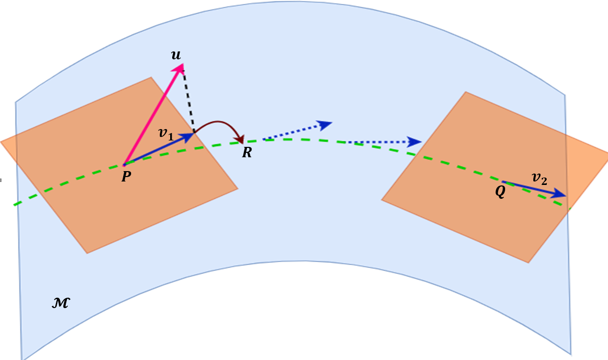
Figure 1: An Illustrative schematic of various operations required in GD-based optimization on Riemannian manifold. Let P and Q represent points on the manifold $\pazocal{M}$ connected by a geodesic shown by the light green dashed curve. The tangent spaces at P and Q, i.e. $T_{\textit{{P}}}\pazocal{M}$ and $T_{\textit{{Q}}}\pazocal{M}$ are shown in orange color. Vector $\textit{{v}}_{1}\in T_{\textit{{P}}}\pazocal{M}$ is the result of the orthogonal projection of the euclidean vector u at P. The retraction operation $\textit{{R}}\!=\!R_{\textit{{P}}}(\textit{{v}}_{1})$ is used to move back to the manifold from the tangent space at P. In a neighborhood of P, the retraction operation (shown in brown) identifies a point on the geodesic. The parallel transport $\textit{{v}}_{2}\!=\!\Gamma_{\textit{{P}}\rightarrow\textit{{Q}}}(\textit{{v}}_{1})$ maps $\textit{{v}}_{1}\in T_{\textit{{P}}}\pazocal{M}$ to $\textit{{v}}_{2}\in T_{\textit{{Q}}}\pazocal{M}$ by parallely moving across the geodesic (as shown in blue dotted arrows) connecting P and Q.

Table 1: The required Riemannian operators for Stiefel manifold, where $\text{Sym}(\textit{{P}})=\frac{1}{2}(\textit{{P}}+\textit{{P}}^{\top})$ and $\text{qf}(\textit{{X}})$ is the $Q$ factor of the $QR$ decomposition of $X$.

Orthogonal projection $\pi_{\textit{{P}}}(\textit{{u}})$	Retraction $R_{\textit{{P}}}(\textit{{v}})$	Parallel transport $\Gamma_{\textit{{P}}\rightarrow\textit{{y}}}(\textit{{w}})$
$\textit{{u}}-\textit{{P}}\text{Sym}(\textit{{P}}^{\top}\textit{{u}})$	$\text{qf}(\textit{{P}}+\textit{{v}})$	$\pi_{\textit{{y}}}(\textit{{w}})$

4 Proposed Method

Generally, the optimization-based meta-training (learn to optimize) problem on Riemannian manifolds can be formulated as [10]:

$$\bm{\Theta}_{meta}^{*}=\underbrace{\min_{\bm{\Theta}\in\pazocal{M}}{\frac{1}{N}\sum_{i=1}^{N}{\pazocal{L}_{i}\big{(}\bm{\pazocal{D}}_{i}^{q},\overbrace{\bm{\Phi}_{i}^{*}}^{\text{inner-level}})}}}_{\text{outer-level}}\big{)}$$ (3)

where $N$ is the number of training tasks, $\bm{\Theta}$ and $\bm{\Phi}_{i}$ respectively indicate the meta-parameters and parameters of the base-learners that are located on a Riemannian manifold $\pazocal{M}$,  i.e $\bm{\Theta},\bm{\Phi}_{i}\in\pazocal{M}$. $\pazocal{L}_{i}$ is the loss function of the $i^{th}$ task, whereas $\pazocal{D}_{i}=\{\bm{\pazocal{D}}_{i}^{s},\bm{\pazocal{D}}_{i}^{q}\}$ demonstrates the meta-train dataset of $i^{th}$ task. The support set $\bm{\pazocal{D}}_{i}^{s}$ and the query set $\bm{\pazocal{D}}_{i}^{q}$ are respectively analogous to training and validation datasets in classic supervised training. The main difference between (3) and the Euclidean meta-learning problem is that each parameter and meta-parameter of the Riemannian meta-learning is a matrix, which is a point on the Riemannian manifold, whereas in Euclidean meta-learning, each parameter or meta-parameter is a vector in Euclidean space. Equation (3) demonstrates two levels of optimization. The outer loop (or the meta-optimizer) learns the optimal meta-parameters,  i.e $\bm{\Theta}_{meta}^{*}$, using query datasets from a distribution of $N$ training tasks and the optimal task-specific parameters $\bm{\Phi}_{i}^{*}$. However, as the $\bm{\Phi}_{i}^{*}$ is unknown, it can be solved as another optimization problem (the inner-level optimization). Therefore, (3) can be considered as a bilevel optimization; a constrained optimization in which each constraint is itself an optimization problem:

$$\begin{split}\bm{\Theta}_{meta}^{*}=\min_{\bm{\Theta}\in\pazocal{M}}{\frac{1}{N}\sum_{i=1}^{N}{\pazocal{L}_{i}\big{(}\bm{\pazocal{D}}_{i}^{q},\bm{\Phi}_{i}^{*}\big{)}}}\\ \text{subject to}~{}~{}\bm{\Phi}_{i}^{*}=\pazocal{G}(\bm{\pazocal{D}}_{i}^{s},\bm{\Theta}_{meta}^{*})\end{split}$$ (4)

where $\pazocal{G}(\bm{\pazocal{D}}_{i}^{s},\bm{\Theta}_{meta}^{*})$ is (usually) a gradient descent optimizer which is dependent on the meta-knowledge, $\bm{\Theta}_{meta}^{*}$. Assuming the meta-parameters as an initial point, the bilevel optimization problem of (4), can be solved by performing two nested loops. At the inner loop, a limited number of gradient descent steps are performed to optimize each task-specific parameter $\bm{\Phi}_{i}^{*}$ using the meta-parameter as an initial point, i.e $\bm{\Phi}_{i}^{(0)}=\bm{\Theta}_{meta}$, and the outer loop performs a gradient descent update for the meta-parameter, $\bm{\Theta}_{meta}$. Each step of the inner loop optimization problem on a Riemannian manifold $\pazocal{M}$ can be formulated as follows:

$$\bm{\Phi}_{i}^{(l+1)}=R_{\bm{\Phi}_{i}^{(l)}}\left(-\alpha\pi_{\bm{\Phi}_{i}^{(l)}}\big{(}\nabla_{\bm{\Phi}_{i}^{(l)}}\pazocal{L}_{i}(\bm{\pazocal{D}}_{i}^{s},\bm{\Phi}_{i}^{(l)})\big{)}\right),l\geq 1$$ (5)

in which the Euclidean gradient vector $\nabla_{\bm{\Phi}_{i}^{(l)}}\pazocal{L}_{i}(\bm{\pazocal{D}}_{i}^{s},\bm{\Phi}_{i}^{(l)})$ is projected to the tangent space of $\bm{\Phi}_{i}^{(l)}$ and then the parameters are updated by performing the retraction operator $R_{\bm{\Phi}_{i}^{(l)}}$.

Moreover, a single step of gradient descent in Riemannian space for the outer loop is as follows:

$$\bm{\Theta}^{(t+1)}=R_{\bm{\Theta}^{(t)}}\left(-\beta\sum_{i=1}^{N}{\pi_{\bm{\Theta}^{(t)}}}\Big{(}\nabla_{\bm{\Theta}^{(t)}}\pazocal{L}_{i}\left(\bm{\pazocal{D}}_{i}^{q},\bm{\Phi}_{i}^{*}\right)\Big{)}\right)$$ (6)

where to calculate $\bm{\Theta}^{(t+1)}$, the Euclidean gradient vector of each task, $\Big{(}\nabla_{\bm{\Theta}^{(t)}}\pazocal{L}_{i}\left(\bm{\pazocal{D}}_{i}^{q},\bm{\Phi}_{i}^{*}\right)\Big{)}$ is orthogonally projected to the tangent space of the current meta-parameter by $\pi_{\bm{\Theta}^{(t)}}(\cdot)$ operation. Then, the summation over the Riemannian gradient of all the tasks is retracted to the manifold. To compute this gradient for each task, differentiating through the inner-level optimization path is needed. In other words, calculating $\pi_{\bm{\Theta}^{(t)}}\Big{(}\nabla_{\bm{\Theta}^{(t)}}\pazocal{L}_{i}\left(\bm{\pazocal{D}}_{i}^{q},\bm{\Phi}_{i}^{*}\right)\Big{)}$ requires computing a gradient of the gradients or second order derivatives which has a high cost and includes backward computations through the Riemannian operators such as retraction and orthogonal projection. Assuming that $k$ Riemannian gradient descent steps are performed in the inner level optimization, then:

$$\nabla_{\bm{\Theta}^{(t)}}\pazocal{L}_{i}\left(\bm{\pazocal{D}}_{i}^{q},\bm{\Phi}_{i}^{*}\right)=\nabla_{\bm{\Theta}^{(t)}}\pazocal{L}_{i}\left(\bm{\pazocal{D}}_{i}^{q},\bm{\Phi}_{i}^{(k)}\right)$$ (7)

where $\bm{\Phi}_{i}^{(k)}$ is the result of inner-level optimization chain:

$$\bm{\Phi}_{i}^{(k)}=R_{\bm{\Phi}_{i}^{(k-1)}}\left(-\alpha\pi_{\bm{\Phi}_{i}^{(k-1)}}\left(\nabla_{\bm{\Phi}_{i}^{(k-1)}}\pazocal{L}_{i}(\bm{\pazocal{D}}_{i}^{s},\bm{\Phi}_{i}^{(k-1)})\right)\right)\\ \bm{\Phi}_{i}^{(k-1)}=R_{\bm{\Phi}_{i}^{(k-2)}}\left(-\alpha\pi_{\bm{\Phi}_{i}^{(k-2)}}\left(\nabla_{\bm{\Phi}_{i}^{(k-2)}}\pazocal{L}_{i}(\bm{\pazocal{D}}_{i}^{s},\bm{\Phi}_{i}^{(k-2)})\right)\right)\\ \vdots\\ \bm{\Phi}_{i}^{(0)}=\bm{\Theta}^{(t)}$$ (8)

Using the chain rule, the derivative in  (7) becomes as follows:

$$\nabla_{\bm{\Theta}^{(t)}}\pazocal{L}_{i}\left(\bm{\pazocal{D}}_{i}^{q},\bm{\Phi}_{i}^{(k)}\right)=\frac{\partial\pazocal{L}_{i}}{\partial\bm{\Phi}_{i}^{(k)}}\frac{\partial\bm{\Phi}_{i}^{(k)}}{\partial\bm{\Theta}^{(t)}}$$ (9)

Considering the inner-level chain of the (9), the $\frac{\partial\bm{\Phi}_{i}^{(k)}}{\partial\bm{\Theta}^{(t)}}$ term can be further unfolded as follows:

$$\nabla_{\bm{\Theta}^{(t)}}\pazocal{L}_{i}\left(\bm{\pazocal{D}}_{i}^{q},\bm{\Phi}_{i}^{(k)}\right)=\frac{\partial\pazocal{L}_{i}\left(\bm{\pazocal{D}}_{i}^{q},\bm{\Phi}_{i}^{(k)}\right)}{\partial\bm{\Phi}_{i}^{(k)}}\prod_{l=1}^{k}{\frac{\partial\bm{\Phi}_{i}^{(l)}}{\partial\bm{\Phi}_{i}^{(l-1)}}}\\ =\frac{\partial\pazocal{L}_{i}\left(\bm{\pazocal{D}}_{i}^{q},\bm{\Phi}_{i}^{(k)}\right)}{\partial\bm{\Phi}_{i}^{(k)}}\\ \prod_{l=1}^{k}{\frac{\partial\bigg{(}R_{\bm{\Phi}_{i}^{(l-1)}}\left(-\alpha\pi_{\bm{\Phi}_{i}^{(l-1)}}\left(\nabla_{\bm{\Phi}_{i}^{(l-1)}}\pazocal{L}_{i}(\bm{\pazocal{D}}_{i}^{s},\bm{\Phi}_{i}^{(l-1)})\right)\right)\bigg{)}}{\partial\bm{\Phi}_{i}^{(l-1)}}}$$ (10)

This equation contains the second-order differentiation terms that pass through the Riemannian operations of the inner-level optimization steps, which requires heavy calculation and computational resources.

In the next section, we formulate a first-order approximation of  (10), that enables us to perform a Hessian-free bi-level optimization for this Riemannian meta-learning problem.

4.1 First order approximation: from Euclidean space to Stiefel manifold

Without loss of generality, let us consider exactly one update step at the inner-level chain of (10). Thus, this step of inner-level optimization will be as follows:

$$\bm{\Phi}_{i}^{(1)}=R_{\bm{\Theta}^{(t)}}\left(-\alpha\pi_{\bm{\Theta}^{(t)}}\left(\nabla_{\bm{\Theta}^{(t)}}\pazocal{L}_{i}(\bm{\pazocal{D}}_{i}^{s},\bm{\Theta}_{i}^{(t)})\right)\right)$$ (11)

Therefore, equation (10) will be reduced to:

$$\nabla_{\bm{\Theta}^{(t)}}\pazocal{L}_{i}\left(\bm{\pazocal{D}}_{i}^{q},\bm{\Phi}_{i}^{(k)}\right)=\\ \frac{\partial\pazocal{L}_{i}\left(\bm{\pazocal{D}}_{i}^{q},\bm{\Phi}_{i}^{(1)}\right)}{\partial\bm{\Phi}_{i}^{(1)}}\frac{\partial\bigg{(}R_{\bm{\Theta}^{(t)}}\left(-\alpha\pi_{\bm{\Theta}^{(t)}}\left(\nabla_{\bm{\Theta}^{(t)}}\pazocal{L}_{i}(\bm{\pazocal{D}}_{i}^{s},\bm{\Theta}^{(t)})\right)\right)\bigg{)}}{\partial\bm{\Theta}^{(t)}}$$ (12)

The above expression applies for all Riemannian manifolds. For instance, using the Euclidian operations on the Euclidean manifold, one can write (12) as:

$$\nabla_{\bm{\theta}^{(t)}}\pazocal{L}_{i}\left(\bm{\pazocal{D}}_{i}^{q},\bm{\phi}_{i}^{(k)}\right)=\\ \frac{\partial\pazocal{L}_{i}\left(\bm{\pazocal{D}}_{i}^{q},\bm{\phi}_{i}^{(1)}\right)}{\partial\bm{\phi}_{i}^{(1)}}\frac{\partial\bigg{(}\bm{\theta}^{(t)}-\alpha(\nabla_{\bm{\theta}^{(t)}}\pazocal{L}_{i}(\bm{\pazocal{D}}_{i}^{s},\bm{\theta}^{(t)})\bigg{)}}{\partial\bm{\theta}^{(t)}}$$ (13)

which can be further simplified to:

$$\nabla_{\bm{\theta}^{(t)}}\pazocal{L}_{i}\left(\bm{\pazocal{D}}_{i}^{q},\bm{\phi}_{i}^{(k)}\right)=\\ \frac{\partial\pazocal{L}_{i}\left(\bm{\pazocal{D}}_{i}^{q},\bm{\phi}_{i}^{(1)}\right)}{\partial\bm{\phi}_{i}^{(1)}}\bigg{(}\bm{I}-\alpha(\nabla^{2}_{\bm{\theta}^{(t)}}\pazocal{L}_{i}(\bm{\pazocal{D}}_{i}^{s},\bm{\theta}^{(t)})\bigg{)}$$ (14)

For the Euclidean spaces, the first-order approximation of (14), FOMAML [11] can be calculated by ignoring its second-order derivatives:

$$\nabla_{\bm{\theta}^{(t)}}\pazocal{L}_{i}\left(\bm{\pazocal{D}}_{i}^{q},\bm{\phi}_{i}^{(k)}\right)=\frac{\partial\pazocal{L}_{i}\left(\bm{\pazocal{D}}_{i}^{q},\bm{\phi}_{i}^{(1)}\right)}{\partial\bm{\phi}_{i}^{(1)}}$$ (15)

On the other hand, calculating such an approximation for the Riemannian spaces is not straightforward. In the rest of this section, we derive the formulation of first-order approximation on Stiefel manifolds. For simplification, we indicate $\nabla_{\bm{\Theta}^{(t)}}\pazocal{L}_{i}(\bm{\pazocal{D}}_{i}^{s},\bm{\Theta}^{(t)})$ as $\nabla_{\bm{\Theta}^{(t)}}\pazocal{L}_{i}$, and $d$ indicates the differential operator. Let us assume that $H^{{}^{\prime}}=\frac{d\bigg{(}R_{\bm{\Theta}^{(t)}}\big{(}-\alpha\pi_{\bm{\Theta}^{(t)}}\left(\nabla_{\bm{\Theta}^{(t)}}\pazocal{L}_{i}(\bm{\pazocal{D}}_{i}^{s},\bm{\Theta}^{(t)})\right)\big{)}\bigg{)}}{d(\bm{\Theta}^{(t)})}$, we aim to compute $H^{{}^{\prime}}$ such that:

$$d\bigg{(}R_{\bm{\Theta}^{(t)}}\big{(}-\alpha\pi_{\bm{\Theta}^{(t)}}\left(\nabla_{\bm{\Theta}^{(t)}}\pazocal{L}_{i}\right)\big{)}\bigg{)}=H^{{}^{\prime}}d(\bm{\Theta}^{(t)})$$ (16)

applying the differential on the left side of (16) and substituting $R_{\bm{P}}(\bm{v})=P+v$ (an approximated version of Stiefel retraction) in that equation results in:

$$d\bigg{(}R_{\bm{\Theta}^{(t)}}\left(-\alpha\pi_{\bm{\Theta}^{(t)}}\left(\nabla_{\bm{\Theta}^{(t)}}\pazocal{L}_{i}\right)\right)\bigg{)}=\\ d\bigg{(}\bm{\Theta}^{(t)}-\alpha\pi_{\bm{\Theta}^{(t)}}\left(\nabla_{\bm{\Theta}^{(t)}}\pazocal{L}_{i}\right)\bigg{)}=\\ d(\bm{\Theta}^{(t)})-d\bigg{(}\alpha\pi_{\bm{\Theta}^{(t)}}\left(\nabla_{\bm{\Theta}^{(t)}}\pazocal{L}_{i}\right)\bigg{)}$$ (17)

considering the Stiefel orthogonal projection $\pi_{\bm{P}}\left(\bm{v}\right)$ from Table 1, equation (17) becomes as follows:

$$d(\bm{\Theta}^{(t)})-\alpha d\bigg{(}\nabla_{\bm{\Theta}^{(t)}}\pazocal{L}_{i}-\bm{\Theta}^{(t)}\frac{(\bm{\Theta}^{(t)})^{T}\nabla_{\bm{\Theta}^{(t)}}\pazocal{L}_{i}-(\nabla_{\bm{\Theta}^{(t)}}\pazocal{L}_{i})^{T}\bm{\Theta}^{(t)}}{2}\bigg{)}\\ =d(\bm{\Theta}^{(t)})-\alpha d(\nabla_{\bm{\Theta}^{(t)}}\pazocal{L}_{i})+0.5\alpha d\bigg{(}\bm{\Theta}^{(t)}(\bm{\Theta}^{(t)})^{T}\nabla_{\bm{\Theta}^{(t)}}\pazocal{L}_{i}\bigg{)}\\ -0.5\alpha d\bigg{(}\bm{\Theta}^{(t)}(\nabla_{\bm{\Theta}^{(t)}}\pazocal{L}_{i})^{T}\bm{\Theta}^{(t)}\bigg{)}$$ (18)

considering $\bm{\Theta}^{(t)}(\bm{\Theta}^{(t)})^{T}=\bm{I}$ for orthogonal matrices, the third part of equation (18) can be further simplified, which results in:

$$d(\bm{\Theta}^{(t)})-\alpha d(\nabla_{\bm{\Theta}^{(t)}}\pazocal{L}_{i})+0.5\alpha d(\nabla_{\bm{\Theta}^{(t)}}\pazocal{L}_{i})\\ -0.5\alpha d\bigg{(}\bm{\Theta}^{(t)}(\nabla_{\bm{\Theta}^{(t)}}\pazocal{L}_{i})^{T}\bm{\Theta}^{(t)}\bigg{)}\\ =d(\bm{\Theta}^{(t)})-0.5\alpha d(\nabla_{\bm{\Theta}^{(t)}}\pazocal{L}_{i})-0.5\alpha d\bigg{(}\bm{\Theta}^{(t)}(\nabla_{\bm{\Theta}^{(t)}}\pazocal{L}_{i})^{T}\bm{\Theta}^{(t)}\bigg{)}$$ (19)

using the relation $d(XYZ)=d(X)YZ+Xd(Y)Z+XYd(Z)$ for the third part of (19), it becomes as follows:

$$d(\bm{\Theta}^{(t)})-0.5\alpha d(\nabla_{\bm{\Theta}^{(t)}}\pazocal{L}_{i})-0.5\alpha d(\bm{\Theta}^{(t)})(\nabla_{\bm{\Theta}^{(t)}}\pazocal{L}_{i})^{T}\bm{\Theta}^{(t)}\\ -0.5\alpha\bm{\Theta}^{(t)}d(\nabla_{\bm{\Theta}^{(t)}}\pazocal{L}_{i})^{T}\bm{\Theta}^{(t)}-0.5\alpha\bm{\Theta}^{(t)}(\nabla_{\bm{\Theta}^{(t)}}\pazocal{L}_{i})^{T}d(\bm{\Theta}^{(t)})$$ (20)

The second and fourth terms of the above formula contain second-order derivatives. By ignoring those terms and using $\operatorname{vec}(\cdot)$ operator, the derivatives with respect to $\bm{\Theta}$ which is an orthogonal matrix (a point on Stiefel manifold) can be written as:

$$\operatorname{vec}\big{(}d(\bm{\Theta}^{(t)})\big{)}-0.5\alpha\operatorname{vec}\big{(}d(\bm{\Theta}^{(t)})(\nabla_{\bm{\Theta}^{(t)}}\pazocal{L}_{i})^{T}\bm{\Theta}^{(t)}\big{)}\\ -0.5\alpha\operatorname{vec}\big{(}\bm{\Theta}^{(t)}(\nabla_{\bm{\Theta}^{(t)}}\pazocal{L}_{i})^{T}d(\bm{\Theta}^{(t)})\big{)}$$ (21)

knowing that $vec(AXB)=(B^{T}\otimes A)vec(X)$, where $\otimes$ indicates the Kronecker product, equation (21) becomes:

$$\bm{I}\operatorname{vec}\big{(}d(\bm{\Theta}^{(t)})\big{)}-0.5\alpha\bigg{(}(\bm{\Theta}^{(t)})^{T}\nabla_{\bm{\Theta}^{(t)}}\pazocal{L}_{i}\otimes\bm{I}\bigg{)}\operatorname{vec}(d(\bm{\Theta}^{(t)}))\\ -0.5\alpha\bigg{(}\bm{I}\otimes\bm{\Theta}^{(t)}(\nabla_{\bm{\Theta}^{(t)}}\pazocal{L}_{i})^{T}\bigg{)}\operatorname{vec}(d(\bm{\Theta}^{(t)}))$$ (22)

using $(A\otimes I)+(I\otimes B)=A\oplus B$, equation (22) can be rewritten as follows:

$$\bigg{(}\bm{I}-0.5\alpha\big{(}(\bm{\Theta}^{(t)})^{T}\nabla_{\bm{\Theta}^{(t)}}\pazocal{L}_{i}\oplus\bm{\Theta}^{(t)}(\nabla_{\bm{\Theta}^{(t)}}\pazocal{L}_{i})^{T}\big{)}\bigg{)}\operatorname{vec}(d(\bm{\Theta}^{(t)}))$$ (23)

in which the symbol $\oplus$ indicates the Kronecker sum. Thus, we will have:

$$\operatorname{vec}\bigg{(}d\bigg{(}R_{\bm{\Theta}^{(t)}}\left(-\alpha\pi_{\bm{\Theta}^{(t)}}\left(\nabla_{\bm{\Theta}^{(t)}}\pazocal{L}_{i}(\bm{\pazocal{D}}_{i}^{s},\bm{\Theta}^{(t)})\right)\right)\bigg{)}\bigg{)}\approx\\ \bigg{(}\bm{I}-0.5\alpha\big{(}(\bm{\Theta}^{(t)})^{T}\nabla_{\bm{\Theta}^{(t)}}\pazocal{L}_{i}\oplus\bm{\Theta}^{(t)}(\nabla_{\bm{\Theta}^{(t)}}\pazocal{L}_{i})^{T}\big{)}\bigg{)}\big{(}\operatorname{vec}(d(\bm{\Theta}^{(t)})\big{)}$$ (24)

As a result:

$$H^{{}^{\prime}}=\bm{I}-0.5\alpha\big{(}(\bm{\Theta}^{(t)})^{T}\nabla_{\bm{\Theta}^{(t)}}\pazocal{L}_{i}\oplus\bm{\Theta}^{(t)}(\nabla_{\bm{\Theta}^{(t)}}\pazocal{L}_{i})^{T}\big{)}$$ (25)

and the first-order approximation of (12) is as follows:

$$\nabla_{\bm{\Theta}^{(t)}}\pazocal{L}_{i}\left(\bm{\pazocal{D}}_{i}^{q},\bm{\Phi}_{i}^{(k)}\right)\approx\frac{\partial\pazocal{L}_{i}\left(\bm{\pazocal{D}}_{i}^{q},\bm{\Phi}_{i}^{(1)}\right)}{\partial\bm{\Phi}_{i}^{(1)}}\\ \bigg{(}\bm{I}-0.5\alpha\big{(}(\bm{\Theta}^{(t)})^{T}\nabla_{\bm{\Theta}^{(t)}}\pazocal{L}_{i}\oplus\bm{\Theta}^{(t)}(\nabla_{\bm{\Theta}^{(t)}}\pazocal{L}_{i})^{T}\big{)}\bigg{)}$$ (26)

Equation (26) computes the derivatives of the outer loop without the need for calculating the Hessian matrices. Moreover, the approximation consists of the Kronecker sum of a matrix with its transpose, which further saves the calculations’ complexity cost.

4.2 Generalization to $k$ inner-level optimization steps

In the previous section, we formulated a first-order approximation for the bi-level meta-learning problem, assuming just one inner-level optimization step. Using (26), it is straightforward to formulate the first-order approximation of (10) as follows:

$$\nabla_{\bm{\Theta}^{(t)}}\pazocal{L}_{i}\left(\bm{\pazocal{D}}_{i}^{q},\bm{\Phi}_{i}^{(k)}\right)\approx\frac{\partial\pazocal{L}_{i}\left(\bm{\pazocal{D}}_{i}^{q},\bm{\Phi}_{i}^{(k)}\right)}{\partial\bm{\Phi}_{i}^{(k)}}\\ \prod_{l=1}^{k}{\bigg{(}\bm{I}-0.5\alpha\big{(}(\bm{\Phi}_{i}^{(l-1)})^{T}\nabla_{\bm{\Phi}_{i}^{(l-1)}}\pazocal{L}_{i}\oplus\bm{\Phi}_{i}^{(l-1)}(\nabla_{\bm{\Phi}_{i}^{(l-1)}}\pazocal{L}_{i})^{T}\big{)}\bigg{)}}$$ (27)

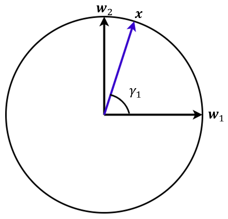
Figure 2: A sample representation of the Stiefel fully connected layer for 2D output space, where $\bm{W}=[\bm{w}_{1},\bm{w}_{2}]$ represents the orthogonal weight matrix (lies on Stiefel manifold) and $\bm{x}$ is the input vector of the Stiefel fully connected layer. For this example, equation (28) becomes: $\bm{W}^{T}\bm{x}=\bm{\gamma}=[\gamma_{1},\gamma_{2}]$.

4.3 The proposed bi-level algorithm

The full proposed method, called FORML, is outlined in Algorithm 1. Practically we meta-optimize the last fully-connected layer of the backbone network using FORML on Stiefel manifold, while the other parameters are optimized on Euclidean space. Moreover, we normalize the input of the Stiefel layer. As a result, the forward computation of the fully-connected layer acts as a cosine similarity between the input vector x and the weight vectors of the classes that are columns of the weight matrix W (as shown in Fig. 2).

$$\textbf{W}^{T}\textbf{x}=\frac{\textbf{W}^{T}\textbf{x}}{\|\textbf{W}\|\|\textbf{x}\|}=\bm{\gamma}$$ (28)

Algorithm 1 FORML

1:$p(\pazocal{T})$ denotes the distribution over meta-training tasks.    $\alpha$ denotes the inner-level learning rate.    $\beta$ represents the outer-level learning rate.

2:Randomly initialize $\bm{\Theta}^{(0)}$

3:while not done do

4:     Sample batch $\{\pazocal{T}_{i}\}_{i=1}^{B}$

5:     for all $\pazocal{T}_{i}$ do

6:         Sample $k$ data points $\bm{\pazocal{D}}_{i}^{s}=\{(\textit{{x}}_{j},\textit{{y}}_{j})\}_{j=1}^{k}$ from $\pazocal{T}_{i}$ for the inner-level updates

7:         Calculate $\nabla_{\bm{\Phi}_{i}^{(l)}}\pazocal{L}_{i}(\bm{\pazocal{D}}_{i}^{s},\bm{\Phi}_{i}^{(l)})$ with respect to $k$ samples.

8:         Compute the task-specific parameters with gradient descent using (5).

9:     end for

10:     Sample $m$ data points $\bm{\pazocal{D}}_{i}^{q}=\{(\textit{{x}}_{j},\textit{{y}}_{j})\}_{j=1}^{m}$ from $\pazocal{T}_{i}$ for the meta-level (outer-level) update

11:     Compute $\nabla_{\bm{\Theta}^{(t)}}\pazocal{L}_{i}\left(\bm{\pazocal{D}}_{i}^{q},\bm{\Phi}_{i}^{(k)}\right)$ using first-order approximation method of (27).

12:     Compute $\bm{\Theta}^{(t+1)}$ using (6).

13:end while

5 Experimental Results

5.1 Evaluation Scenarios and Datasets

We evaluate our proposed method across different few-shot classification tasks. Following the experimental setting provided by [10, 21], we address both single-domain and cross-domain scenarios. In the single-domain experiments, the meta-train, meta-validation, and meta-test tasks are sampled from one dataset, while in the cross-domain scenarios, the meta-test tasks are from a different dataset. Thereby the effect of domain shift in our proposed method is also studied in this scenario.

5.1.1 Single-domain image classification

To address the single-domain scenario, we conduct two experiments including object recognition and fine-grained image classification. Mini-ImageNet [22] is used for object recognition, which includes a subset of 100 classes from the ImageNet dataset [23] and 600 images are sampled from each class. Following the setting provided by Ravi and Larochelle [22], the dataset is split into randomly selected 64, 16, and 20 classes for meta-train, meta-validation and meta-test, respectively.

For fine-grained image classification, we use the CUB-200-2011 (CUB) [24] and FC100 [25] datasets. The CUB dataset consists of 11,788 images belonging to 200 different classes of birds. Following the evaluation protocol of [26], the dataset is randomly divided into the train, validation, and test meta-sets with 100, 50, and 50 classes respectively. The FC100 dataset is based on the popular object classification dataset CIFAR100 [25] and offers a more challenging few-shot scenario, because of lower image resolution and using more challenging meta-training/test splits that are separated according to the object superclasses. The dataset contains 100 object classes and each class has 600 samples of 32×32 color images. These 100 classes belong to 20 superclasses. Following the splits proposed by Krizhevsky et al. [25], meta-training data contain 60 classes from 12 super-classes. Meta-validation and meta-test sets are from 20 classes belonging to 4 super-classes, respectively. Splitting the data according to the super-classes minimizes the information overlap between training and validation/test tasks.

5.1.2 Cross-domain image classification

One key aspect of few-shot experiments is investigating the effect of domain shift between the meta-train and meta-test datasets on the meta-learning algorithm. For instance, one can observe that the domain gap between the meta-train and meta-test classes of miniImageNet is larger than that of CUB in the word-net hierarchy [27]. Thus, meta-learning on miniImageNet is more challenging than the CUB dataset. Hence, we also address the cross-domain scenarios in our experimental setup. The cross-domain experiment enables us to study the effect of domain shift on our proposed method, although our method was originally developed for single-domain classification.

Following the scenarios provided by other state-of-the-art works [21], we conduct mini-ImageNet$\rightarrow$CUB and Omniglot$\rightarrow$EMNIST cross-domain experiments. For the mini-ImageNet$\rightarrow$CUB experiment, all of the $100$ classes of mini-ImageNet are used as meta-train set, while 50 meta-validation and 50 meta-test classes are sampled from CUB. For Omniglot$\rightarrow$EMNIST experiment, we follow the setting proposed by Dong and Xing [28], where the non-Latin characters of Omniglot dataset are used as the meta-train classes, and the EMNIST dataset [29] that contains 10-digits and upper and lower case alphabets in English, is used for our meta-validation and meta-test classes. In total, the meta-train set consists of 1597 classes from the Omniglot dataset, while the 62 classes of EMNIST are split into 31 classes for meta-validation and 31 classes for meta-test sets.

5.2 Experimental Details

We use the standard $N\text{-way}$ $k\text{-shot}$ classification setups, in which every task instance contains randomly sampled classifying images from $N$ different categories of the meta-train set. For each class, we sample $k$ instances as our support set and $q$ instances for the query set. For the meta-test phase, we run 600 experiments and report the average classification accuracy and the 95% confidence interval of these 600 trials as the final result. $N$, $k$, and $q$ are sampled similarly to the meta-train stage. In our experiments, $N$ is set to 5 for all of the experiments across all datasets.

For mini-ImageNet and CUB datasets, we use four-layer and six-layer convolutional backbones (Conv-4 and Conv-6) with an input size of $84\times 84$. We also use the ResNet-10 and ResNet-18 backbone networks with an input size of $224\times 224$. For the FC100 experiment, we use Conv-4 and ResNet-12 backbone networks. We also use Conv-4 for cross-domain character recognition (Omniglot$\rightarrow$EMNIST) experimental setup, while ResNet-18 network is used for the mini-ImageNet$\rightarrow$CUB experiment.

In all of the experiments across every network backbone, we assume that the parameters of the last fully connected layer of the network are orthonormal and lie on a Stiefel manifold. FORML meta-learns this matrix using the Riemannian operators, as described in Algorithm 1. FORML optimizes the parameters of the remaining layers in Euclidean space. All of the experiments were performed on a single NVIDIA V100 GPU with a 32GB of video memory.

5.2.1 Hyper-parameter setups

Table 2 introduces the notation used for the Steifel and Euclidean hyper-parameters. In the single-domain setup:

• $\alpha$ is set to $0.1$ for experiments with Conv-4 and COnv-6 backbone architecture, while it is set to $0.01$ for the others.

• $\widehat{\beta}$ is set to $10^{-3}$ for all experiments with Conv-4 and Conv-6 backbones architecture.

• $\widehat{\beta}$ is set to $10^{-4}$ for experiments using ResNet backbone architectures.

Similarly, for the experiments in the cross-domain setup:

• the value of $\alpha$ is set to $0.01$ for mini-ImageNet$\rightarrow$CUB, and is set to $0.05$ and $0.1$ for Omniglot$\rightarrow$EMNIST 1-shot and 5-shot experiments, respectively.

• $\widehat{\beta}$ for mini-ImageNet$\rightarrow$CUB is set $5\times 10^{-4}$, while it is set to $10^{-3}$ and $10^{-4}$ for Omniglot$\rightarrow$EMNIST 1-shot and 5-shot experiments, respectively.

For all experiments, the learning rate $\widetilde{\beta}$ is set to $10^{-3}$. All hyper-parameters are obtained by trial and error and for all experiments, the batch size and the number of inner-level updates for training are always set to 4 and 5, respectively.

Table 2: Notations and descriptions of hyper-parameters for experiments with FORML.

Learning Rate	Parameters	Loop
$\alpha$	Stiefel layer	Inner
$\widetilde{\beta}$	Stiefel layer	Outer
$\widehat{\beta}$	Euclidean layer	Outer

Table 3: A comparison of few-shot classification accuracies between first-order approximation methods in Euclidean space (MAML) and Stiefel manifold (FORML) for mini-ImageNet and CUB datasets against different backbone networks is shown in the last 3 columns. 5-way classification setting is used in all experiments. The best results are shown in bold.

Dataset	Method	Conv-4	Conv-6	ResNet-10
CUB 1-shot	MAML (First-Order) [21]	$54.73\pm 0.97$	$66.26\pm 1.05$	$70.32\pm 0.99$
	FORML (ours)	$\bm{58.86\pm 0.99}$	$\bm{67.29\pm 0.99}$	$\bm{70.96\pm 0.97}$
CUB 5-shot	MAML (First-Order) [21]	$75.75\pm 0.76$	$78.82\pm 0.70$	$80.93\pm 0.71$
	FORML (ours)	$\bm{77.93\pm 0.95}$	$\bm{79.76\pm 0.98}$7	$82.45\pm 0.69$
mini-ImageNet 1-shot	MAML (First-Order)[21]	$46.47\pm 0.82$	$50.96\pm 0.92$	$54.69\pm 0.89$
	FORML (ours)	$49.94\pm 0.84$	$51.68\pm 0.55$	$55.13\pm 0.88$
mini-ImageNet 5-shot	MAML (First-Order) [21]	$62.71\pm 0.71$	$66.09\pm 0.71$	$66.62\pm 0.83$
	FORML (ours)	$65.46\pm 0.68$	$68.12\pm 0.88$	$68.82\pm 0.85$

Table 4: Few-shot classification accuracies for mini-ImageNet datasets against Conv-4 backbone network. 5-way classification setting is used in all experiments. The best results are shown in bold.

Method	1-shot	5-shot
MAML (first-0order) [21]	$46.47\pm 0.82$	$62.71\pm 0.71$
Reptile [16]	$47.07\pm 0.26$	$62.74\pm 0.38$
ANIL [12]	$47.20\pm 0.27$	$62.59\pm 0.39$
BOIL [13]	$47.76\pm 0.31$	$64.40\pm 0.28$
RMAML [10]	$50.03\pm 0.84$	$65.12\pm 0.76$
FORML (ours)	$49.94\pm 0.84$	$65.46\pm 0.68$

Table 5: Results of Few-shot classification results on CUB dataset using Conv-4 backbone. The best results are shown in bold.

Method	1-shot	5-shot
ANIL [12]	$47.20\pm 0.27$	$62.59\pm 0.39$
BOIL [13]	$47.76\pm 0.31$	$64.40\pm 0.28$
RMAML[10]	$75.79\pm 0.92$	$86.77\pm 0.57$
FORML (ours)	$\bm{74.86\pm 0.92}$	$86.35\pm 0.78$

Table 6: Few-shot classification accuracies for FC100 dataset. 5-way classification setting is used in all experiments. The best results are shown in bold.

Backbone Networks	Conv-4		ResNet-12
Method	1-shot	5-shot	1-shot	5-shot
Baseline	$32.48\pm 0.58$	$47.15\pm 0.67$	$38.24\pm 0.63$	$56.87\pm 0.71$
MAML	$36.70\pm 0.83$	$47.69\pm 0.79$	$40.15\pm 0.78$	$54.13\pm 0.77$
ANIL [12]	$36.37\pm 0.33$	$45.65\pm 0.44$	-	-
BOIL [13]	$38.93\pm 0.45$	$51.66\pm 0.32$	-	-
RMAML [10]	$39.92\pm 0.64$	$51.34\pm 0.72$	$42.58\pm 0.70$	$59.68\pm 0.78$
FORML (ours)	$38.82\pm 0.72$	$49.05\pm 0.88$	$41.30\pm 0.68$	$57.35\pm 0.84$

Table 7: Few-shot classification accuracies for mini-ImageNet datasets against Conv-4 backbone network. 5-way classification setting is used in all experiments. The best results are shown in bold.

Method	1-shot	5-shot
ML-LSTM [30]	$43.44\pm 0.77$	$60.60\pm 0.71$
iMAML-HF [31]	$49.30\pm 1.88$	-
Meta-Mixture [32]	$49.60\pm 1.50$	$64.60\pm 0.92$
Amortized VI [33]	$44.13\pm 1.78$	$55.68\pm 0.91$
DKT+BNCosSim [34]	$49.73\pm 0.07$	$64.00\pm 0.09$
FORML (ours)	$49.94\pm 0.84$	$65.46\pm 0.68$

Table 8: Supplementary comparison for Few-shot classification results on CUB dataset using ResNet-18 backbone. The best results are shown in bold.

Method	1-shot	5-shot
Robust-20 [35]	$58.67\pm 0.70$	$75.62\pm 0.50$
GNN-LFT [36]	$51.51\pm 0.80$	$73.11\pm 0.68$
Baseline++ [21]	$67.02\pm 0.90$	$83.58\pm 0.50$
Arcmax [37]	$71.37\pm 0.90$	$85.74\pm 0.50$
MixtFSL [38]	$73.94\pm 1.10$	$86.01\pm 0.50$
RMAML[10]	$75.79\pm 0.92$	$86.77\pm 0.57$
FORML (ours)	$\bm{74.86\pm 0.92}$	$86.35\pm 0.78$

Table 9: Supplementary comparison for few-shot classification results on FC100 dataset. The best results are shown in bold.

Method	Backbone	1-shot	5-shot
MetaOptNet [39]	ResNet-12	$41.10\pm 0.60$	$55.50\pm 0.60$
Arcmax [37]	ResNet-18	$40.84\pm 0.71$	$57.02\pm 0.63$
MixtFSL [38]	ResNet-18	$41.50\pm 0.67$	$58.39\pm 0.62$
FORML (ours)	ResNet-12	$41.30\pm 0.68$	$57.35\pm 0.84$

5.3 Results for Single-Domain Experiments

We examined our proposed method against single-domain few-shot classification benchmarks including mini-ImageNet, CUB, and FC100 benchmarks. All experiments are conducted for the standard 5-way 1-shot and 5-shot classification. Table 3 compares the few-shot classification results between the first-order MAML and FORML with different backbone networks, against mini-ImageNet and CUB datasets. To have a fair comparison, FORML utilizes the same hyperparameter setting as MAML. Among all the experimental setups, FORML shows a significant improvement over its non-Riemannian counterpart (i.e MAML) in terms of classification accuracy. Moreover, the presented results demonstrate the robustness of FORML against deeper backbones.

We also compare our method against its non-approximation-based version, RMAML [10], and two other types of methods including the approximation-based methods [11, 16] and methods that focus on increasing the representation reuse or representation change [12, 13]. As this set of methods includes the Euclidean and Riemannian counterparts of FORML, it is important to compare them fairly. Thus, all experiments of FORML are conducted with the same hyperparameter settings as used for those methods. For Mini-ImageNet, Table 4 demonstrates the effectiveness of FORML against the approximation methods (First-order MAML and Reptile). In addition, our proposed method shows superiority against ANIL and BOIL methods. Compared to its non-approximation-based version, RMAML, which is based on second-order gradients, FORML achieves a higher classification accuracy ($65.46\pm 0.68$ vs $65.12\pm 0.76$) in 5-shot classification, while obtains a competitive results in 1-shot classification. As presented in Table 5, for the fine-grained dataset CUB, the proposed method outperforms all the considered methods on both 1-shot settings. In 5-shot experiments, FORML beats ANIL and BOIL methods and archives a competitive result, compared to RMAML.

Adopting Conv-4 and ResNet-12 backbones, we also assess our algorithm against the FC100 benchmark. As shown in Table 6, we observe that FORML improves the few-shot recognition performance on the FC100 dataset, compared to MAML and other methods. Surprisingly, our proposed method achieves competitive accuracy compared to other state-of-the-art methods on the FC100 dataset, as depicted in Table 9.

Overall, single-domain experimental results show that using the same hyperparameters and setting, our proposed technique outperforms the original MAML and another approximation-based extension of MAML. Also, FORML demonstrates competitive results compared to its Riemannian non-approximation-based version, RMAML. Using the orthogonality constraints in the head of the models in FORML that limits the parameter search space, leads to higher performance and better convergence. Moreover, learning the cosine similarity between the input and the parameters of the head, facilitates the convergence and the adaptation of the head toward the optimum.

Table 10: Classification accuracies for Omniglot$\rightarrow$EMNIST and mini-ImageNet$\rightarrow$CUB cross-domain experimental setup.

	Omniglot$\rightarrow$EMNIST		mini-ImageNet$\rightarrow$CUB
Backbone Networks	Conv-4		ResNet-18
Method	1-shot	5-shot	5-shot
Baseline	$63.94\pm 0.87$	$86.00\pm 0.59$	$65.57\pm 0.70$
MAML	$72.04\pm 0.83$	$88.24\pm 0.56$	$51.34\pm 0.72$
FORML (ours)	$72.78\pm 0.82$	$87.41\pm 0.57$	$56.43\pm 0.71$

5.3.1 Further Assessment and Comparison

To further verify the effectiveness of our approach, we continue to compare FORML with more few-shot learning algorithms. Tables 7, 8 and 9 illustrate the results on mini-ImageNet, CUB and FC100 datasets, respectively. As presented in Table 7, FORML outperforms all the previous state-of-the-art algorithms for 5-shot classification on the mini-ImageNet dataset. We also observe that our algorithm improves the few-shot recognition performance on the CUB dataset compared to the considered methods. The proposed algorithm is compared with several state-of-the-art methods with ResNet-18 backbone. The results show that FORML outperforms all the considered methods on both 1-shot and 5-shot settings. In addition, RMAML outperforms all of the state-of-the-art algorithms for 5-shot classification on FC100 dataset.

5.4 Results for Cross-Domain Experiments

We adopt mini-ImageNet$\rightarrow$CUB and Omniglot$\rightarrow$EMNIST scenarios for the cross-domain experiments. The results of mini-ImageNet$\rightarrow$CUB and Omniglot$\rightarrow$EMNIST experiments are demonstrated in Table 10. For the 1-shot Omniglot$\rightarrow$EMNIST experiment, FORML outperforms all other methods as shown in Table 10, while still obtaining comparable results to that of MAML for the 5-shot experiment. Moreover, FORML has remarkably outperformed FOMAML by more than $5\%$, in terms of classification accuracy in the mini-ImageNet$\rightarrow$CUB experiment. However, as depicted in Table 10, all methods are outperformed by the baseline. This is because the representation reuse in FORML fails to overcome the diverse and significant domain gap between the meta-train and meta-test sets, while for the baseline method (which is a transfer learning method [21]) is much simpler to adapt to the target domain by learning a new parameterized classifier layer  [23, 21, 10]. Despite this fact, FORML still obtains competitive results in terms of classification accuracy against other methods.

5.5 Time and Memory Consumption

To demonstrate the efficiency of our method, we also measured both time and video memory consumption during the meta-training, and compared them with its Euclidean (MAML) and non-approximation-based Riemannian (RMAML) counterparts, as depicted in Tables 11 and 12. To do so, we utilized FORML (our proposed method), RMAML (the Riemannian non-approximation-based method), MAML (the Euclidean counterpart of RMAML), FOMAML (first-order approximation of MAML) to train a Conv-4 backbone on CUB dataset with the same hyperparameters such as number of inner-level steps, inner-level and outer-level learning rates and batch-size. The Results suggest that using FORML saves a tangible amount of time and memory as compared to its non-approximated version, RMAML. Moreover, although FORML uses Riemannian operations which are computationally expensive, it has a competitive memory usage and runtime as compared to Eucleadian methods.

We also measured the time consumption of the baselearner and the meta-learner. The time consumption of the baselearner was measured over the forward process of the inner-loop, and the time consumption of the meta-learner was measured over the backward processes. As illustrated in Table 12, the execution time of one epoch of FORML is more than 3 times faster than RMAML. It also performs the inner-loop 20 times faster than RMAML. In comparison with its Euclidean counterparts, FORML performed an epoch 12 times faster and the outer-loop updates 16 times faster than MAML, and achieved competitive runtime and memory usage compared to FOMAML.

Table 11: Memory consumption

Method	Memory (MB)
MAML (first-0order)	$7.3\times 10^{3}$
MAML	$1.81\times 10^{3}$
RMAML	$7.86\times 10^{3}$
FORML (ours)	$1.94\times 10^{3}$

Table 12: Total Execution time and average time of the inner and outer loops of 1 iteration (100 iterations)

Method	Execution time (seconds)	Avg. Inner-loop (seconds)	Avg. outer-loop (seconds)
MAML (first-0order)	$7.62$	$6.09\times 10^{-2}$	$4.23\times 10^{-3}$
MAML	$31.86$	$6.19\times 10^{-2}$	$9.31\times 10^{-1}$
RMAML	$39.80$	$9.50\times 10^{-2}$	$1.16$
FORML (ours)	$12.14$	$9.03\times 10^{-2}$	$5.81\times 10^{-2}$

6 Conclusion

This paper introduced FORML, a first-order approximation method for meta-learning on Stiefel manifolds. FORML formulates a Hessian-free bi-level optimization, which reduces the optimization-based Riemannian meta-learning’s computational cost and memory usage, and suppresses the overfitting phenomena. Using FORML to meta-learn an orthogonal fully-connected layer as the head of the backbone model, where its parameters are cast on the Stiefel manifold, has amplified the representation reuse of the model during the meta-learning. By normalizing the input of the classification layer, a similarity vector between the input of the head and the class-specific parameters is calculated. As a result, the model learns how to move the head input toward the desired class. We conducted two experimental scenarios: single-domain and cross-domain few-shot classification. The results have demonstrated the superiority of FORML against its Euclidean counterpart, MAML, by a significant margin, while achieving competitive results against other meta-learning methods. We also compared FORML with its Riemannian and Euclidean counterparts in terms of GPU memory usage and execution time. Our proposed method demonstrates a significant improve over its non-approximation-based version, RMAML, by performing an epoch and an inner-level optimization loop more than 3 times and 20 times faster, respectievly. It also shows a remarkable improve over MAML and a competitive performance compared with FOMAML.

Motivated by the observed results, we aim to develop a multi-modal or multi-task Riemannian meta-learning method in the future, that will be able to effectively tackle the cross-domain or even cross-modal scenarios.

Hadi Tabealhojeh is a Ph.D. candidate of Artificial Intelligence and Robotics working under supervision of Dr. Peyman Adibi and Dr. Hossein Karshenas in Artificial Intelligence Department, Faculty of Computer Engineering, University of Isfahan, Isfahan, Iran. He received his M.Sc. degree from Shahid Chamran University of Ahvaz, Ahvaz, Iran. He is currently a member of Intelligent and Learning Systems Research Lab. His current research interests include Deep Learning, Meta-Learning and multi-modal learning, especially on curved and non-linear spaces and their applications. Currently, He is a lecturer at the Department of Computer Engineering, Faculty of Engineering, Shahid Chamran universit of Ahvaz. Soumava Kumar Roy received his Ph.D. degree from the College of Engineering and Computer Science, Australian National University in 2021. Prior to this, he received his bachelor’s of engineering degree in electronics and communication engineering from the Manipal Institute of Technology, Manipal, India, in 2013, and the master’s of technology degree in Information Technology from the Indian Institute of Information Technology, Allahabad, India. His research interests include deep learning and computer vision. He is currently working as a post doctoral researcher in the Computer Vision Lab, EPFL. Peyman Adibi received the Ph.D. degree from Faculty of Computer Engineering, Amirkabir University of Technology, Tehran, Iran. He is currently an Associate Professor at Artificial Intelligence Department, Faculty of Computer Engineering, University of Isfahan, where he is the head of Intelligent and Learning Systems Research Lab. He was a visiting Professor at GIPSA Lab, Grenoble Institute of Technology, Grenoble, France, in 2016-2017. His current research interests include Machine Learning and Pattern Recognition, Multimodal and Geometric Learning, Computer Vision and Image Processing, Computational Intelligence and Soft Computing, and their applications. Hossein Karshenas received his BE degree in computer engineering from Shahid Beheshti University, Tehran, Iran, in 2006 and ME degree in artificial intelligence and robotics from Iran University of Science and Technology (IUST), Tehran, Iran, in 2009. He received his PhD degree in artificial intelligence from Technical University of Madrid (UPM), Madrid, Spain, in 2013. He is currently an assistant professor at the artificial intelligence department, faculty of computer engineering, University of Isfahan, Isfahan, Iran. His main research interests include estimation of distribution algorithms, computational intelligence, data analytics and modeling and multi-objective optimization where he has published several articles in peer-reviewed journals.

References

- [1] T. Hospedales, A. Antoniou, P. Micaelli, and A. Storkey, “Meta-learning in neural networks: A survey,” IEEE transactions on pattern analysis and machine intelligence, vol. 44, no. 9, pp. 5149–5169, 2021.
- [2] J. Yuan and A. Lamperski, “Online adaptive principal component analysis and its extensions,” in International Conference on Machine Learning. PMLR, 2019, pp. 7213–7221.
- [3] A. Hyvärinen and E. Oja, “Independent component analysis: algorithms and applications,” Neural networks, vol. 13, no. 4-5, pp. 411–430, 2000.
- [4] R. Chakraborty, L. Yang, S. Hauberg, and B. C. Vemuri, “Intrinsic grassmann averages for online linear, robust and nonlinear subspace learning,” IEEE transactions on pattern analysis and machine intelligence, vol. 43, no. 11, pp. 3904–3917, 2020.
- [5] N. Bansal, X. Chen, and Z. Wang, “Can We Gain More from Orthogonality Regularizations in Training Deep CNNs?” arXiv preprint arXiv:1810.09102, 2018.
- [6] M. Cogswell, F. Ahmed, R. Girshick, L. Zitnick, and D. Batra, “Reducing Overfitting in Deep Networks by Decorrelating Representations,” arXiv preprint arXiv:1511.06068, 2015.
- [7] Z. Huang, J. Wu, and L. Van Gool, “Building Deep Networks on Grassmann Manifolds,” in Proceedings of the AAAI Conference on Artificial Intelligence, vol. 32, no. 1, 2018.
- [8] T. Lin and H. Zha, “Riemannian manifold learning,” IEEE transactions on pattern analysis and machine intelligence, vol. 30, no. 5, pp. 796–809, 2008.
- [9] S. K. Roy, Z. Mhammedi, and M. Harandi, “Geometry aware constrained optimization techniques for deep learning,” in Proceedings of the IEEE conference on computer vision and pattern recognition, 2018, pp. 4460–4469.
- [10] H. Tabealhojeh, P. Adibi, H. Karshenas, S. K. Roy, and M. Harandi, “Rmaml: Riemannian meta-learning with orthogonality constraints,” Pattern Recognition, vol. 140, p. 109563, 2023.
- [11] C. Finn, P. Abbeel, and S. Levine, “Model-agnostic meta-learning for fast adaptation of deep networks,” in International conference on machine learning. PMLR, 2017, pp. 1126–1135.
- [12] A. Raghu, M. Raghu, S. Bengio, and O. Vinyals, “Rapid learning or feature reuse? towards understanding the effectiveness of maml,” in International Conference on Learning Representations, 2019.
- [13] J. Oh, H. Yoo, C. Kim, and S. Yun, “Boil: Towards representation change for few-shot learning,” in The Ninth International Conference on Learning Representations (ICLR). The International Conference on Learning Representations (ICLR), 2021.
- [14] Z. Gao, Y. Wu, Y. Jia, and M. Harandi, “Learning to optimize on spd manifolds,” in Proceedings of the IEEE/CVF Conference on Computer Vision and Pattern Recognition, 2020, pp. 7700–7709.
- [15] Z. Gao, Y. Wu, X. Fan, M. Harandi, and Y. Jia, “Learning to optimize on riemannian manifolds,” IEEE Transactions on Pattern Analysis and Machine Intelligence, 2022.
- [16] A. Nichol, J. Achiam, and J. Schulman, “On first-order meta-learning algorithms,” arXiv preprint arXiv:1803.02999, 2018.
- [17] X. Fan, Z. Gao, Y. Wu, Y. Jia, and M. Harandi, “Learning a gradient-free riemannian optimizer on tangent spaces,” in Proceedings of the AAAI Conference on Artificial Intelligence, vol. 35, no. 8, 2021, pp. 7377–7384.
- [18] P.-A. Absil, R. Mahony, and R. Sepulchre, Optimization Algorithms on Matrix Manifolds. Princeton University Press, 2009.
- [19] W. M. Boothby, An introduction to differentiable manifolds and Riemannian geometry. Academic press, 1986.
- [20] N. Qian, “On the Momentum Term in Gradient Descent Learning Algorithms,” Neural networks, vol. 12, no. 1, pp. 145–151, 1999.
- [21] W.-Y. Chen, Y.-C. Liu, Z. Kira, Y.-C. F. Wang, and J.-B. Huang, “A closer look at few-shot classification,” in International Conference on Learning Representations, 2019.
- [22] S. Ravi and H. Larochelle, “Optimization as a Model for Few-Shot Learning,” 2016.
- [23] O. Vinyals, C. Blundell, T. Lillicrap, D. Wierstra et al., “Matching Networks for One Shot Learning,” Advances in neural information processing systems, vol. 29, pp. 3630–3638, 2016.
- [24] C. Wah, S. Branson, P. Welinder, P. Perona, and S. Belongie, “The Caltech-ucsd Birds-200-2011 Dataset,” 2011.
- [25] A. Krizhevsky, G. Hinton et al., “Learning multiple layers of features from tiny images,” 2009.
- [26] N. Hilliard, L. Phillips, S. Howland, A. Yankov, C. D. Corley, and N. O. Hodas, “Few-Shot Learning with Metric-Agnostic Conditional Embeddings,” arXiv preprint arXiv:1802.04376, 2018.
- [27] G. A. Miller, “Wordnet: A Lexical Database for English,” Communications of the ACM, vol. 38, no. 11, pp. 39–41, 1995.
- [28] N. Dong and E. P. Xing, “Domain Adaption in One-Shot Learning,” in Joint European Conference on Machine Learning and Knowledge Discovery in Databases. Springer, 2018, pp. 573–588.
- [29] G. Cohen, S. Afshar, J. Tapson, and A. Van Schaik, “EMNIST: Extending MNIST to Handwritten Letters,” in 2017 International Joint Conference on Neural Networks (IJCNN). IEEE, 2017, pp. 2921–2926.
- [30] S. Ravi and H. Larochelle, “Optimization as a model for few-shot learning,” in In International Conference on Learning Representations (ICLR), 2017.
- [31] A. Rajeswaran, C. Finn, S. M. Kakade, and S. Levine, “Meta-Learning with Implicit Gradients,” in Proceedings of the 33rd International Conference on Neural Information Processing Systems, 2019, pp. 113–124.
- [32] G. Jerfel, E. Grant, T. Griffiths, and K. A. Heller, “Reconciling meta-learning and continual learning with online mixtures of tasks,” Advances in Neural Information Processing Systems, vol. 32, 2019.
- [33] J. Gordon, J. Bronskill, M. Bauer, S. Nowozin, and R. E. Turner, “Meta-learning probabilistic inference for prediction,” in ICLR (Poster), 2019.
- [34] M. Patacchiola, J. Turner, E. J. Crowley, M. O’Boyle, and A. J. Storkey, “Bayesian meta-learning for the few-shot setting via deep kernels,” Advances in Neural Information Processing Systems, vol. 33, pp. 16 108–16 118, 2020.
- [35] N. Dvornik, C. Schmid, and J. Mairal, “Diversity with cooperation: Ensemble methods for few-shot classification,” in Proceedings of the IEEE/CVF international conference on computer vision, 2019, pp. 3723–3731.
- [36] H.-Y. Tseng, H.-Y. Lee, J.-B. Huang, and M.-H. Yang, “Cross-domain few-shot classification via learned feature-wise transformation,” arXiv preprint arXiv:2001.08735, 2020.
- [37] A. Afrasiyabi, J.-F. Lalonde, and C. Gagné, “Associative alignment for few-shot image classification,” in Computer Vision–ECCV 2020: 16th European Conference, Glasgow, UK, August 23–28, 2020, Proceedings, Part V 16. Springer, 2020, pp. 18–35.
- [38] ——, “Mixture-based feature space learning for few-shot image classification,” in Proceedings of the IEEE/CVF International Conference on Computer Vision, 2021, pp. 9041–9051.
- [39] K. Lee, S. Maji, A. Ravichandran, and S. Soatto, “Meta-learning with differentiable convex optimization,” in Proceedings of the IEEE/CVF conference on computer vision and pattern recognition, 2019, pp. 10 657–10 665.