Binding-Adaptive Diffusion Models for Structure-Based Drug Design
Abstract
Structure-based drug design (SBDD) aims to generate 3D ligand molecules that bind to specific protein targets. Existing 3D deep generative models including diffusion models have shown great promise for SBDD. However, it is complex to capture the essential protein-ligand interactions exactly in 3D space for molecular generation. To address this problem, we propose a novel framework, namely Binding-Adaptive Diffusion Models (BindDM). In BindDM, we adaptively extract subcomplex, the essential part of binding sites responsible for protein-ligand interactions. Then the selected protein-ligand subcomplex is processed with SE(3)-equivariant neural networks, and transmitted back to each atom of the complex for augmenting the target-aware 3D molecule diffusion generation with binding interaction information. We iterate this hierarchical complex-subcomplex process with cross-hierarchy interaction node for adequately fusing global binding context between the complex and its corresponding subcomplex. Empirical studies on the CrossDocked2020 dataset show BindDM can generate molecules with more realistic 3D structures and higher binding affinities towards the protein targets, with up to -5.92 Avg. Vina Score, while maintaining proper molecular properties. Our code is available at https://github.com/YangLing0818/BindDM
Introduction
Designing ligand molecules that can bind to specific protein targets and modulate their function, also known as structure-based drug design (SBDD) (Anderson 2003; Batool, Ahmad, and Choi 2019), is a fundamental problem in drug discovery and can lead to significant therapeutic benefits. SBDD requires models to synthesize drug-like molecules with stable 3D structures and high binding affinities to the target. Nevertheless, it is challenging and involves massive computational efforts because of the enormous space of synthetically feasible chemicals (Ragoza, Masuda, and Koes 2022a) and freedom degree of both compound and protein structures (Hawkins 2017).
Recent advances in modeling geometric structures of biomolecules (Bronstein et al. 2021; Atz, Grisoni, and Schneider 2021) motivate a promising direction for SBDD (Gaudelet et al. 2021; Zhang et al. 2023b). Several new generative methods have been proposed for the SBDD task (Li, Pei, and Lai 2021; Luo et al. 2021; Peng et al. 2022; Powers et al. 2022; Ragoza, Masuda, and Koes 2022b; Zhang et al. 2023a), which learn to generate ligand molecules by modeling the complex spatial and chemical interaction features of the binding site. For instance, some methods adopt autoregressive models (ARMs) (Luo and Ji 2021; Liu et al. 2022a; Peng et al. 2022) and show promising results in SBDD tasks, which generate 3D molecules by iteratively adding atoms or bonds based on the target binding site. However, ARMs tend to suffer from error accumulation, and it also is difficult to find an optimal generation order.
An alternative to address these limitations of ARMs is to sample the atomic coordinates and types of all the atoms at once (Du et al. 2022). Recent diffusion-based SBDD methods (Guan et al. 2023a; Schneuing et al. 2023; Lin et al. 2022; Guan et al. 2023b) adopt diffusion models (Ho, Jain, and Abbeel 2020; Song et al. 2020) to model the distribution of atom types and positions from a standard Gaussian prior with post-processing to assign bonds. These diffusion-based methods learn the joint generative process with a SE(3)-equivariant diffusion models (Hoogeboom et al. 2022) to capture both spatial and chemical interactions between atoms, and have achieved comparable performance with previous autoregressive models.
Despite the state-of-the-art performance, existing methods pay little attention to the binding-specific substructure of protein-ligand complex, i.e., the essential part of binding sites responsible for protein-ligand interactions, which plays a crucial role in generating molecules with high binding affinities towards the protein targets (Bajusz et al. 2021; Kozakov et al. 2015). Although recent FLAG (Zhang et al. 2023a) and DrugGPS (Zhang and Liu 2023) learn to generate pocket-aware 3D molecules fragment-by-fragment, these massive pre-defined fragments (e.g., motifs or subpockets) are still complex for the model to exactly discover essential protein-ligand interactions from highly diverse protein pockets in nature (Spitzer, Cleves, and Jain 2011; Basanta et al. 2020). Consequently, these limit their practical use in designing high-affinity molecules for new protein targets.
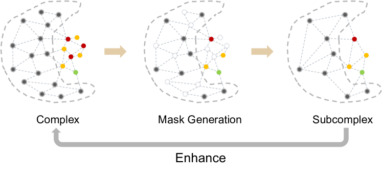
To address these issues, we propose BindDM, a new binding-adaptive diffusion model for SBDD. Instead of using pre-defined fragments of pockets or molecules (e.g., subpockets or motifs), at each time step of denoising process, we directly extract essential binding subcomplex from protein-ligand complex with a learnable structural pooling. Then we process the selected subcomplex with SE(3)-equivariant GNNs, and transmit them back to the complex as enhanced binding context to improve the atomic target-aware 3D molecule generation. To facilitate the exchange between the complex and its subcomplex, we iterate the above process via our designed cross-hierarchy interaction nodes. Extensive experiments demonstrate that BindDM can generate molecules with more realistic 3D structures and higher binding affinities towards the protein targets, while maintaining proper molecular properties. We highlight our main contributions as follows:
-
•
We propose a hierarchical complex-subcomplex diffusion model for structure-based drug design, which incorporates essential binding-adaptive subcomplex for 3D molecule diffusion generation.
-
•
We design and incorporate cross-hierarchy interaction nodes into our iterative denoising networks in the generation process for sufficiently fusing context information.
-
•
Empirical results on CrossDocked2020 dataset demonstrate that our BindDM achieves better performance compared with previous methods, higher affinity with target protein and other drug properties.
Related Work
Structure-Based Drug Design
As the increasing availability of 3D-structure protein-ligand data (Kinnings et al. 2011), structure-based drug design (SBDD) becomes a hot research area and it aims to generate diverse molecules with high binding affinity to specific protein targets (Luo et al. 2021; Yang et al. 2022b; Schneuing et al. 2023; Tan, Gao, and Li 2023). Early attempts learn to generate SMILES strings or 2D molecular graphs given protein contexts (Skalic et al. 2019; Xu, Ran, and Chen 2021). However, it is uncertain whether the resulting compounds with generated strings or graphs could really fit the geometric landscape of the 3D structural pockets. More works start to involve 3D structures of both proteins and molecules (Li, Pei, and Lai 2021; Ragoza, Masuda, and Koes 2022b; Zhang et al. 2023a). Luo et al. (2021), Liu et al. (2022b), and Peng et al. (2022) adopt autoregressive models to generate 3D molecules in an atom-wise manner. Recently, powerful diffusion models (Sohl-Dickstein et al. 2015; Song and Ermon 2019; Ho, Jain, and Abbeel 2020) begin to play a role in SBDD, and have achieved promising generation results with non-autoregressive sampling (Lin et al. 2022; Schneuing et al. 2023; Guan et al. 2023a). TargetDiff (Guan et al. 2023a), DiffBP (Lin et al. 2022), and DiffSBDD (Schneider et al. 1999) utilize E(n)-equivariant GNNs (Satorras, Hoogeboom, and Welling 2021) to parameterize conditional diffusion models for protein-aware 3D molecular generation. Despite progress, existing methods pay little attention to binding-specific protein-ligand substructures. In contrast, We propose BindDM to automatically extracts essential binding-adaptive subcomplex, and design a hierarchical equivariant molecular diffusion model for SBDD.
Diffusion Models for SBDD
As a new family of deep generative models, diffusion models (Sohl-Dickstein et al. 2015; Ho, Jain, and Abbeel 2020; Song et al. 2020; Yang et al. 2022a, 2023c, 2023a) have been recently applied in SBDD tasks. They usually represent the protein-ligand complex by treating protein binding pockets and ligand molecules as atom point sets in the 3D space, and define a diffusion process for both continuous atom coordinates and discrete atom types for reverse diffusion generation. TargetDiff (Guan et al. 2023a) and DiffBP (Lin et al. 2022) both propose a target-aware molecular diffusion process with a SE(3)-equivariant GNN denoiser. DecompDiff (Guan et al. 2023b) proposes a two-stage diffusion model, which uses an open-source software to obtain molecule-agnostic binding priors as templates for the generation process. In contrast, our BindDM is a single-stage approach that generates molecules from scratch without relying on external knowledge. It adaptively mines binding-related subcomplexes from the original complex to enhance the generation process, fully considering the interaction between protein pockets and ligands.
Preliminary
The SBDD task from the perspective of generative models can be defined as generating molecules which can bind to a given protein pocket. The target protein and molecule can be represented as and , respectively. Here (resp. ) refers to the number of atoms of the protein (resp. the molecule ). and denote the position and type of the atom, respectively. And denotes the number of atom types. In the sequel, matrices are denoted by uppercase boldface. For a matrix , denotes the vector on its -th row, and denotes the submatrix comprising its -st to -th rows. For brevity, the molecule is denoted as where and , and the protein is denoted as where and . The task can be formulated as modeling the conditional distribution .
Denoising Diffusion Probabilistic Models (DDPMs) equipped with SE(3)-invariant prior and SE(3)-equivariant transition kernel have been applied on the SBDD task (Guan et al. 2023a; Schneuing et al. 2023; Lin et al. 2022). Specifically, types and positions of the ligand molecule are modeled by DDPM, while the number of atoms is usually sampled from an empirical distribution (Hoogeboom et al. 2022; Guan et al. 2023a) or predicted by a neural network (Lin et al. 2022), and bonds are determined as post-processing.
In the forward diffusion process, a small Gaussian noise is gradually injected into data as a Markov chain. Because noises are only added on ligand molecules but not proteins in the diffusion process, we denote the atom positions and types of the ligand molecule at time step as and and omit the subscript without ambiguity. The diffusion transition kernel can be defined as follows:
| (1) | ||||
where and stand for the Gaussian and categorical distribution respectively, is defined by fixed variance schedules. The corresponding posterior can be derived as follows:
| (2) | ||||
where , , , , , and .
In the approximated reverse process, also known as the generative process, a neural network parameterized by learns to recover data by iteratively denoising. The reverse transition kernel can be approximated with predicted atom types and atom positions as follows:
| (3) | ||||
The Proposed BindDM
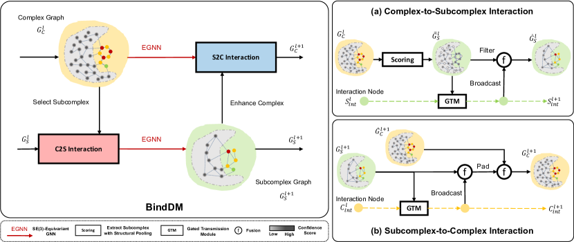
As discussed in previous sections, we aim to develop a hierarchical binding-specific diffusion model for SBDD. We here present our proposed BindDM, as illustrated in Figure 2. In this subsection, we will describe how to introduce the selected protein-ligand binding subcomplex into the design of the neural network which predicts (i.e., reconstructs) in the reverse generation process:
| (4) |
To extract essential interaction binding-adaptive protein-ligand subcomplex, we design a learnable structural pooling to filter the nodes in the original complex graph. To sufficiently utilize both the complex and the subcomplex, we apply SE(3)-equivariant neural networks on them. Finally, we design cross-hierarchy interaction nodes to iteratively exchange information between the complex and the subcomplex, and facilitate the target-aware 3D molecule generation.
Binding-Adaptive Subcomplex Extraction
We first elaborate on how we adaptively extract essential binding subcomplex at each time step . Different from the denoising networks in previous SBDD methods (Guan et al. 2023a, b; Schneuing et al. 2023) that only process the full-atom complex graph, our BindDM produces a binding-adaptive subcomplex graph from the complex graph with a learnable structural pooling. Formally, we have a -nearest neighbors graph based on the protein-ligand complex at each denoising time step, where the superscripts denotes the -th graph layer of the denoising network, and denotes the concatenation along the first dimension. We aim to extract a binding subcomplex graph from (and , for ), where is the node hidden state matrix (initialized with in first layer), is the node position matrix. We calculate the confidence scores of all nodes in the complex graph contributing to the molecule generation with provided binding sites:
| (5) | ||||
| (6) |
where is the adjacency matrix with pair-wise node connections defined on -nn graph according to , is the degree matrix of , is an MLP, is the learnable parameter, is the operation of filling empty nodes into the position of filtered nodes according to the indices of selected nodes. In this way, the padded subcomplex graph has the same number of nodes as the complex graph. The is indices of the top nodes which are selected based on confidence scores , and is the selection ratio that determines the number of nodes to keep:
| (7) |
where the top-rank is the function that returns the indices of the top values. In practice, we set . Then, the hidden state matrix and position matrix of subcomplex are obtained:
| (8) | ||||
| (9) |
where is an indexing operation, is the broadcasted elementwise product, and are the row-wise (i.e. node-wise) indexed matrix and , respectively. Next, we process the selected subcomplex to better leverage binding context for molecule generation.
3D Equivariant Complex-Subcomplex Processing
Our goal is to generate 3D molecules based on target protein binding sites, the model needs to generate both continuous atom coordinates and discrete atom types, while being SE(3)-equivariant to global translation and rotation during the entire generative process. This property is a critical inductive bias for generating 3D molecules (Hoogeboom et al. 2022; Schneuing et al. 2023; Guan et al. 2023a), and an invariant distribution composed with an equivariant transition function will result in an invariant distribution. Thus, for our hierarchical complex-subcomplex denoising network, we have the following proposition in the setting of protein-aware molecule generation.
Proposition 1.
Denoting SE(3)-transformation as , we can achieve invariant likelihood w.r.t on both the protein-ligand complex and its subcomplex: if we shift the Center of Mass (CoM) of protein atoms to zero and parameterize the Markov transition with a SE(3)-equivariant network.
We apply two SE(3)-equivariant neural networks on the -nn graphs ( and ) of the protein-ligand complex and its corresponding subcomplex in the denoising process, respectively. For the subcomplex graph updated through the complex-to-subcomplex (C2S) interaction, the SE(3)-invariant hidden states and SE(3)-equivariant positions are updated as follows to obtain the :
| (10) | ||||
where is the set of -nearest neighbors of atom on the subcomplex graph, indicates the atom and atom are both protein atoms or both ligand atoms or one protein atom and one ligand atom, and is the ligand atom mask since the protein atom coordinates are known and thus supposed to remain unchanged during this update. The similar process are applied on the complex graph to obtained the .
Iterative Cross-Hierarchy Interaction
In BindDM, we introduce two cross-hierarchy interaction nodes to facilitate the information exchange between the binding contexts of two hierarchies, the complex graph and its subcomplex graph. Specifically, we initialize the interaction node of subcomplex graph via sum pooling:
| (11) |
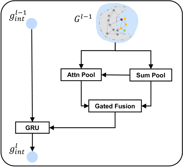
Then the binding context of the extracted subcomplex graph is transmitted back to the complex graph for cross-hierarchy information fusion via the interaction node and the gated transmission module as shown in Figure 3:
| (12) | |||
| (13) | |||
| (14) | |||
| (15) |
where is sigmoid, , and are MLPs, is the SE(3)-invariant hidden state of -th node in . Equations 12, 13 and 14 mix the messages between the subcomplex graph and the interaction node through gated recurrent unit (GRU) (Chung et al. 2014) for updating . Equation 15 perform node-wise fusion with for subcomplex-to-complex (S2C) interaction. Similarly, we also have the interaction node for complex-to-subcomplex (C2S) interaction, and we iterate these cross-hierarchy processes for sufficiently incorporating binding-adaptive subcomplex into the 3D molecule generation process as shown in Figure 2.
Training and Sampling
To train BindDM (i.e., optimize the evidence lower bound induced by BindDM), we use the same objective function as Guan et al. (2023a). The atom position loss and atom type loss at time step are defined as follows respectively:
| (16) | ||||
| (17) |
where and are predicted from and , and . Kindly recall that , , , and correspond to the -th row of , , , and , respectively. The final loss is a weighted sum of atom coordinate loss and atom type loss with a hyperparameter as: .
Experiments
Experimental Settings
Datasets and Baseline Methods
As for molecular generation, following the previous work (Luo et al. 2021; Peng et al. 2022; Guan et al. 2023a), we train and evaluate BindDM on the CrossDocked2020 dataset (Francoeur et al. 2020). Adhering to the data preparation and splitting procedures outlined by Luo et al. (2021), we refine the million docked binding complexes to high-quality docking poses (RMSD between the docked pose and the ground truth Å) and diverse proteins (sequence identity ). This meticulous process produces protein-ligand pairs for training and proteins for testing. We compare our model against four recent representative methods for SBDD. LiGAN (Ragoza, Masuda, and Koes 2022a) is a conditional VAE model trained on an atomic density grid representation of protein-ligand structures. AR (Luo et al. 2021) and Pocket2Mol (Peng et al. 2022) are autoregressive schemes that generate 3D molecules atoms conditioned on the protein pocket and previous generated atoms. TargetDiff (Guan et al. 2023a) and DecompDiff (Guan et al. 2023b) represent state-of-the-art diffusion methods, generating atom coordinates and atom types in a non-autoregressive manner.
Evaluation
We conduct a comprehensive assessment of the generated molecules, evaluating them from three key perspectives: molecular structures, target binding affinity, and molecular properties. In terms of molecular structures, we quantify the Jensen-Shannon divergences (JSD) in empirical distributions of atom/bond distances between the generated molecules and the reference ones. To evaluate the target binding affinity, following previous work (Luo et al. 2021; Ragoza, Masuda, and Koes 2022b; Guan et al. 2023a), we adopt AutoDock Vina (Eberhardt et al. 2021) to compute and report the mean and median of binding-related metrics, including Vina Score, Vina Min, Vina Dock and High Affinity. Vina Score directly estimates the binding affinity; Vina Min involves local structure minimization before estimation; Vina Dock integrates an additional re-docking process for optimal binding affinity; High affinity measures the ratio of generated molecules binding better than the reference molecule per test protein. To evaluate molecular properties, we utilize QED, SA, Diversity as metrics following Luo et al. (2021); Ragoza, Masuda, and Koes (2022a). QED is a quantitative estimation of drug-likeness combining several desirable molecular properties; SA (synthesize accessibility) estimates the difficulty of synthesizing the ligands; Diversity is computed as average pairwise dissimilarity between all generated ligands. All sampling and evaluation procedures follow Guan et al. (2023a) for fair comparison.
Bond liGAN AR Pocket2 Mol Target Diff Decomp Diff Ours CC 0.601 0.609 0.496 0.369 0.359 0.380 CC 0.665 0.620 0.561 0.505 0.537 0.229 CN 0.634 0.474 0.416 0.363 0.344 0.265 CN 0.749 0.635 0.629 0.550 0.584 0.245 CO 0.656 0.492 0.454 0.421 0.376 0.329 CO 0.661 0.558 0.516 0.461 0.374 0.249 CC 0.497 0.451 0.416 0.263 0.251 0.282 CN 0.638 0.552 0.487 0.235 0.269 0.130
Methods Vina Score () Vina Min () Vina Dock () High Affinity () QED () SA () Diversity () Avg. Med. Avg. Med. Avg. Med. Avg. Med. Avg. Med. Avg. Med. Avg. Med. Reference -6.36 -6.46 -6.71 -6.49 -7.45 -7.26 - - 0.48 0.47 0.73 0.74 - - LiGAN - - - - -6.33 -6.20 21.1% 11.1% 0.39 0.39 0.59 0.57 0.66 0.67 GraphBP - - - - -4.80 -4.70 14.2% 6.7% 0.43 0.45 0.49 0.48 0.79 0.78 AR -5.75 -5.64 -6.18 -5.88 -6.75 -6.62 37.9% 31.0% 0.51 0.50 0.63 0.63 0.70 0.70 Pocket2Mol -5.14 -4.70 -6.42 -5.82 -7.15 -6.79 48.4% 51.0% 0.56 0.57 0.74 0.75 0.69 0.71 TargetDiff -5.47 -6.30 -6.64 -6.83 -7.80 -7.91 58.1% 59.1% 0.48 0.48 0.58 0.58 0.72 0.71 DecompDiff -5.67 -6.04 -7.04 -6.91 -8.39 -8.43 64.4% 71.0% 0.45 0.43 0.61 0.60 0.68 0.68 BindDM -5.92 -6.81 -7.29 -7.34 -8.41 -8.37 64.8% 71.6% 0.51 0.52 0.58 0.58 0.75 0.74
Main Results
Generated 3D Molecular Structures
We compare our BindDM and the representative methods in terms of molecular structures. We compute different bond distributions of the generated molecules and compare them against the corresponding reference empirical distributions in Tab. 1. Our model has a comparable performance with TargetDiff and DecompDiff and substantially outperforms all other baselines across all major bond types, indicating the great potential of BindDM for generating stable molecular structures.
Target Binding Affinity and Molecule Properties
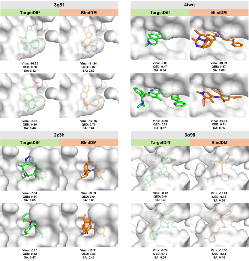
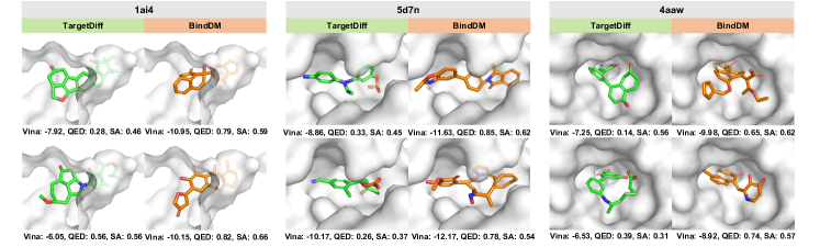
We evaluate the effectiveness of BindDM in terms of binding affinity. We can see in Tab. 2 that our BindDM outperforms baselines in binding-related metrics. Specifically, BindDM surpasses strong autoregressive method Pocket2Mol by a large margin of 15.2%, 13.6% and 17.6% in Avg. Vina Score, Vina Min and Vina Dock, respectively. Compared with the state-of-the-art diffusion-based method DecompDiff, BindDM not only increased the binding-related metrics Avg. Vina Score and Vina Min by 4.4% and 3.6%, respectively, but also significantly increased the property-related metric Avg. QED by 13.3%. In terms of high-affinity binder, we find that on average 64.8% of the BindDM molecules show better binding affinity than the reference molecule, which is significantly better than other baselines. These gains demonstrate that the proposed BindDM effectively captures significant binding-related subcomplex to enable generating molecules with improved target binding affinity. Moreover, we can see a trade-off between property-related metrics QED and binding-related metrics in previous methods. DecompDiff performs better than AR and Pocket2Mol in binding-related metrics, but falls behind them in QED scores. In contrast, our BindDM not only achieves the state-of-the-art binding-related scores but also maintains proper QED score, achieving a better trade-off than DecompDiff. Nevertheless, we put less emphasis on QED and SA because they are often applied as rough screening metrics in real drug discovery scenarios, and it would be fine as long as they are within a reasonable range. Figure 4 shows some examples of generated ligand molecules and their properties. The molecules generated by our model have valid structures and reasonable binding poses to the target, which are supposed to be promising candidate ligands.
Model Analysis
Effect of the Iterative Cross-Hierarchy Interaction on Target-specific Molecule Generation
We conduct a set of ablation experiments to study the effect of iterative cross-hierarchy interaction on the generation ability of diffusion models for the target-specific molecules: (1) Exp0: the baseline model without applying the iterative cross-hierarchy interaction, (2) Exp1: we replace the binding-adaptive subcomplex extraction (BASE) module with a random selection of atoms from the complex for constructing the subcomplex. The selection ratio is set to 0.5, (3) Exp2: we remove subcomplex graphs in iterative cross-hierarchy interaction and keep interaction nodes unchanged for information propagation between cross-layer complex graphs, (4) Exp3: we remove interaction nodes and and keep the extracted subcomplex graphs unchanged, (5) Exp4: we remove the gated transmission module in the update of interaction nodes and . The results are present in Tab. 3.
In the comparison between Exp0 and Exp1, we can find that randomly selected subcomplex can not provide useful information about pocket-ligand binding. And the comparison between Exp1 and BindDM suggests that BASE is more effective than random selection in exploring binding-related clues from the complex. The effectiveness of BASE is beneficial for BindDM in generating molecules that are tightly bound to the given protein pocket. In comparing Exp2 with BindDM, it is evident that solely relying on global interaction nodes for information propagation between cross-layer complex graphs does not provide significant binding-related information for pocket-specific molecular generation. In comparing Exp3 with BindDM, we observe that the utilization of global interaction nodes for information exchange between complex and subcomplex not only improves the performance of BindDM in binding-related metrics but also contributes to the molecular property-related ones. And the same conclusion is also observed in the comparison between Exp4 and BindDM.
Methods Vina Score () Vina Min () Vina Dock () QED () Avg. Med. Avg. Med. Avg. Med. Avg. Med. Exp0 -5.04 -5.75 -6.38 -6.52 -7.55 -7.72 0.46 0.46 Exp1 -4.79 -5.92 -6.36 -6.66 -7.71 -7.63 0.50 0.51 Exp2 -5.65 -6.25 -6.64 -6.65 -7.96 -7.77 0.45 0.45 Exp3 -5.62 -6.74 -6.83 -6.92 -8.11 -8.15 0.47 0.46 Exp4 -5.60 -6.28 -6.78 -6.83 -7.94 -8.01 0.47 0.47 BindDM -5.92 -6.81 -7.29 -7.34 -8.41 -8.37 0.51 0.52
Influence of Extracting Binding Clues from Complex, Pocket and Ligand
Since the presence of binding clues in both the molecular ligands and protein pockets, we conduct three experiments to explore the effects of extracting binding-related clues from different structures on how tightly the generated molecules bind to the specific protein pockets: the binding-related substructures are extracted from (1) the molecular ligands, (2) the protein pockets, and (3) the complexes (treating the molecule and pocket as a unified entity) to enhance the generation of molecular ligands binding tightly to specific protein pockets, respectively. As present in Tab. 4, BindDM can achieve the best performance on binding-related metrics when binding-related substructures are extracted from complexes and used to enhance the generation process of protein-specific molecular ligands.
Methods Vina Score () Vina Min () Vina Dock () QED () Avg. Med. Avg. Med. Avg. Med. Avg. Med. baseline -5.04 -5.75 -6.38 -6.52 -7.55 -7.72 0.46 0.46 Pocket -5.37 -6.84 -7.03 -7.38 -8.30 -8.36 0.51 0.52 Ligand -5.46 -6.77 -6.98 -7.27 -8.13 8.29 0.51 0.52 Complex -5.92 -6.81 -7.29 -7.34 -8.41 -8.37 0.51 0.52
Correlation between Adaptively Extracted Subcomplex and Pocket-Ligand Binding Clues
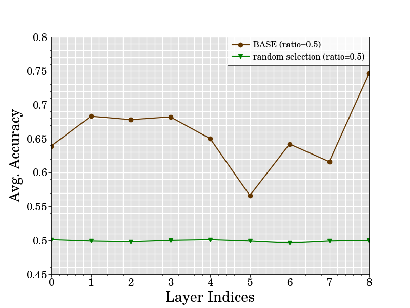
To validate the presence of binding-related clues in the subcomplex extracted by BASE in BindDM and their suitability for generating molecular ligands tightly bound to specific protein pockets, we initially employed the pre-trained binding affinity prediction model BAPNet (Li, Pei, and Lai 2021). By predicting binding affinity of the complex which consists of the given protein pocket and the molecules generated by BindDM, the binding-related subcomplex is obtained by ranking the complex atoms according to contributions to the binding affinity prediction. We take the subcomplexes predicted by BAPNet as the reference subcomplexes, and calculate the accuracy of the subcomplexes predicted by BASE as a metric to assess the effectiveness of BASE in extracting binding-related subcomplex. Considering that the sampling process consists of 1000 steps, we calculate the average accuracy by comparing the reference subcomplex with all the subcomplexes extracted by each layer of the denoising network in BindDM (9 layers in total) throughout the entire sampling process. As shown in Figure 5, each layer of the denoising network of BindDM achieves an accuracy rate of around 0.65 for subcomplex extracted through BASE, which is higher than the accuracy rate of around 0.5 for random selection (in practice, the selection ratio is set to 0.5). This suggests that BASE in BindDM is capable of extracting binding-related subcomplex to a certain degree. In addition, we replace the process of using BASE to adaptively select binding-related subcomplex with randomly selecting atoms from the complex to construct a substructure. The performance present in Tab. 3 (Exp1) demonstrates the subcomplex extracted from BASE benefit the final performance.
Conclusion
In this paper, we propose an effective diffusion model BindDM to adaptively extract the essential part of binding sites responsible for protein-ligand interactions, subcomplex, for enhancing protein-aware 3D molecule generation. We further design cross-hierarchy interaction node to facilitate the hierarchical information exchange between complex and subcomplex. Empirical results sufficiently demonstrate BindDM can generate more realistic 3D molecules with higher binding affinities towards the protein targets, while maintaining proper molecular properties. For future work, we will extend our BindDM to few-shot scenarios (Yang et al. 2020) by leveraging recent advances in graph representation learning (Yang et al. 2023b; Yang and Hong 2022).
Acknowledgement
The work was partly supported by the National Natural Science Foundation of China (No.62171251), the Major Key Project of GZL under Grant SRPG22-001 and the Major Key Project of PCL under Grant PCL2023A09.
References
- Anderson (2003) Anderson, A. C. 2003. The process of structure-based drug design. Chemistry & biology, 10(9): 787–797.
- Atz, Grisoni, and Schneider (2021) Atz, K.; Grisoni, F.; and Schneider, G. 2021. Geometric deep learning on molecular representations. Nature Machine Intelligence, 3(12): 1023–1032.
- Bajusz et al. (2021) Bajusz, D.; Wade, W. S.; Satała, G.; Bojarski, A. J.; Ilaš, J.; Ebner, J.; Grebien, F.; Papp, H.; Jakab, F.; Douangamath, A.; et al. 2021. Exploring protein hotspots by optimized fragment pharmacophores. Nature Communications, 12(1): 3201.
- Basanta et al. (2020) Basanta, B.; Bick, M. J.; Bera, A. K.; Norn, C.; Chow, C. M.; Carter, L. P.; Goreshnik, I.; Dimaio, F.; and Baker, D. 2020. An enumerative algorithm for de novo design of proteins with diverse pocket structures. Proceedings of the National Academy of Sciences, 117(36): 22135–22145.
- Batool, Ahmad, and Choi (2019) Batool, M.; Ahmad, B.; and Choi, S. 2019. A structure-based drug discovery paradigm. International journal of molecular sciences, 20(11): 2783.
- Bronstein et al. (2021) Bronstein, M. M.; Bruna, J.; Cohen, T.; and Veličković, P. 2021. Geometric Deep Learning: Grids, Groups, Graphs, Geodesics, and Gauges. arXiv:2104.13478.
- Chung et al. (2014) Chung, J.; Gulcehre, C.; Cho, K.; and Bengio, Y. 2014. Empirical Evaluation of Gated Recurrent Neural Networks on Sequence Modeling. arXiv:1412.3555.
- Du et al. (2022) Du, Y.; Fu, T.; Sun, J.; and Liu, S. 2022. MolGenSurvey: A Systematic Survey in Machine Learning Models for Molecule Design. arXiv:2203.14500.
- Eberhardt et al. (2021) Eberhardt, J.; Santos-Martins, D.; Tillack, A. F.; and Forli, S. 2021. AutoDock Vina 1.2. 0: New docking methods, expanded force field, and python bindings. Journal of Chemical Information and Modeling, 61(8): 3891–3898.
- Francoeur et al. (2020) Francoeur, P. G.; Masuda, T.; Sunseri, J.; Jia, A.; Iovanisci, R. B.; Snyder, I.; and Koes, D. R. 2020. Three-dimensional convolutional neural networks and a cross-docked data set for structure-based drug design. Journal of Chemical Information and Modeling, 60(9): 4200–4215.
- Gaudelet et al. (2021) Gaudelet, T.; Day, B.; Jamasb, A. R.; Soman, J.; Regep, C.; Liu, G.; Hayter, J. B.; Vickers, R.; Roberts, C.; Tang, J.; et al. 2021. Utilizing graph machine learning within drug discovery and development. Briefings in bioinformatics, 22(6): bbab159.
- Guan et al. (2023a) Guan, J.; Qian, W. W.; Peng, X.; Su, Y.; Peng, J.; and Ma, J. 2023a. 3D Equivariant Diffusion for Target-Aware Molecule Generation and Affinity Prediction. In International Conference on Learning Representations.
- Guan et al. (2023b) Guan, J.; Zhou, X.; Yang, Y.; Bao, Y.; Peng, J.; Ma, J.; Liu, Q.; Wang, L.; and Gu, Q. 2023b. DecompDiff: Diffusion Models with Decomposed Priors for Structure-Based Drug Design. In Krause, A.; Brunskill, E.; Cho, K.; Engelhardt, B.; Sabato, S.; and Scarlett, J., eds., Proceedings of the 40th International Conference on Machine Learning, volume 202 of Proceedings of Machine Learning Research, 11827–11846. PMLR.
- Hawkins (2017) Hawkins, P. C. 2017. Conformation generation: the state of the art. Journal of Chemical Information and Modeling, 57(8): 1747–1756.
- Ho, Jain, and Abbeel (2020) Ho, J.; Jain, A.; and Abbeel, P. 2020. Denoising diffusion probabilistic models. Advances in Neural Information Processing Systems, 33: 6840–6851.
- Hoogeboom et al. (2022) Hoogeboom, E.; Satorras, V. G.; Vignac, C.; and Welling, M. 2022. Equivariant diffusion for molecule generation in 3d. In International conference on machine learning, 8867–8887. PMLR.
- Kinnings et al. (2011) Kinnings, S. L.; Liu, N.; Tonge, P. J.; Jackson, R. M.; Xie, L.; and Bourne, P. E. 2011. A machine learning-based method to improve docking scoring functions and its application to drug repurposing. Journal of chemical information and modeling, 51(2): 408–419.
- Kozakov et al. (2015) Kozakov, D.; Hall, D. R.; Jehle, S.; Luo, L.; Ochiana, S. O.; Jones, E. V.; Pollastri, M.; Allen, K. N.; Whitty, A.; and Vajda, S. 2015. Ligand deconstruction: Why some fragment binding positions are conserved and others are not. Proceedings of the National Academy of Sciences, 112(20): E2585–E2594.
- Li, Pei, and Lai (2021) Li, Y.; Pei, J.; and Lai, L. 2021. Structure-based de novo drug design using 3D deep generative models. Chemical science, 12(41): 13664–13675.
- Lin et al. (2022) Lin, H.; Huang, Y.; Liu, M.; Li, X.; Ji, S.; and Li, S. Z. 2022. DiffBP: Generative Diffusion of 3D Molecules for Target Protein Binding. arXiv:2211.11214.
- Liu et al. (2022a) Liu, M.; Luo, Y.; Uchino, K.; Maruhashi, K.; and Ji, S. 2022a. Generating 3D Molecules for Target Protein Binding. In International Conference on Machine Learning.
- Liu et al. (2022b) Liu, M.; Luo, Y.; Uchino, K.; Maruhashi, K.; and Ji, S. 2022b. Generating 3D Molecules for Target Protein Binding. arXiv:2204.09410.
- Luo et al. (2021) Luo, S.; Guan, J.; Ma, J.; and Peng, J. 2021. A 3D generative model for structure-based drug design. Advances in Neural Information Processing Systems, 34: 6229–6239.
- Luo and Ji (2021) Luo, Y.; and Ji, S. 2021. An autoregressive flow model for 3d molecular geometry generation from scratch. In International Conference on Learning Representations.
- Peng et al. (2022) Peng, X.; Luo, S.; Guan, J.; Xie, Q.; Peng, J.; and Ma, J. 2022. Pocket2mol: Efficient molecular sampling based on 3d protein pockets. In International Conference on Machine Learning, 17644–17655. PMLR.
- Powers et al. (2022) Powers, A. S.; Yu, H. H.; Suriana, P.; and Dror, R. O. 2022. Fragment-based ligand generation guided by geometric deep learning on protein-ligand structure. bioRxiv, 2022–03.
- Ragoza, Masuda, and Koes (2022a) Ragoza, M.; Masuda, T.; and Koes, D. R. 2022a. Generating 3D molecules conditional on receptor binding sites with deep generative models. Chem Sci, 13: 2701–2713.
- Ragoza, Masuda, and Koes (2022b) Ragoza, M.; Masuda, T.; and Koes, D. R. 2022b. Generating 3D molecules conditional on receptor binding sites with deep generative models. Chemical science, 13(9): 2701–2713.
- Satorras, Hoogeboom, and Welling (2021) Satorras, V. G.; Hoogeboom, E.; and Welling, M. 2021. E (n) equivariant graph neural networks. In International conference on machine learning, 9323–9332. PMLR.
- Schneider et al. (1999) Schneider, G.; Neidhart, W.; Giller, T.; and Schmid, G. 1999. “Scaffold-hopping” by topological pharmacophore search: a contribution to virtual screening. Angewandte Chemie International Edition, 38(19): 2894–2896.
- Schneuing et al. (2023) Schneuing, A.; Du, Y.; Harris, C.; Jamasb, A.; Igashov, I.; Du, W.; Blundell, T.; Lió, P.; Gomes, C.; Welling, M.; Bronstein, M.; and Correia, B. 2023. Structure-based Drug Design with Equivariant Diffusion Models. arXiv:2210.13695.
- Skalic et al. (2019) Skalic, M.; Jiménez, J.; Sabbadin, D.; and De Fabritiis, G. 2019. Shape-based generative modeling for de novo drug design. Journal of chemical information and modeling, 59(3): 1205–1214.
- Sohl-Dickstein et al. (2015) Sohl-Dickstein, J.; Weiss, E.; Maheswaranathan, N.; and Ganguli, S. 2015. Deep unsupervised learning using nonequilibrium thermodynamics. In International Conference on Machine Learning, 2256–2265. PMLR.
- Song and Ermon (2019) Song, Y.; and Ermon, S. 2019. Generative modeling by estimating gradients of the data distribution. Advances in Neural Information Processing Systems, 32.
- Song et al. (2020) Song, Y.; Sohl-Dickstein, J.; Kingma, D. P.; Kumar, A.; Ermon, S.; and Poole, B. 2020. Score-Based Generative Modeling through Stochastic Differential Equations. In International Conference on Learning Representations.
- Spitzer, Cleves, and Jain (2011) Spitzer, R.; Cleves, A. E.; and Jain, A. N. 2011. Surface-based protein binding pocket similarity. Proteins: Structure, Function, and Bioinformatics, 79(9): 2746–2763.
- Tan, Gao, and Li (2023) Tan, C.; Gao, Z.; and Li, S. Z. 2023. Target-aware molecular graph generation. In Joint European Conference on Machine Learning and Knowledge Discovery in Databases, 410–427. Springer.
- Xu, Ran, and Chen (2021) Xu, M.; Ran, T.; and Chen, H. 2021. De novo molecule design through the molecular generative model conditioned by 3D information of protein binding sites. Journal of Chemical Information and Modeling, 61(7): 3240–3254.
- Yang and Hong (2022) Yang, L.; and Hong, S. 2022. Omni-granular ego-semantic propagation for self-supervised graph representation learning. In International Conference on Machine Learning, 25022–25037. PMLR.
- Yang et al. (2022a) Yang, L.; Huang, Z.; Song, Y.; Hong, S.; Li, G.; Zhang, W.; Cui, B.; Ghanem, B.; and Yang, M.-H. 2022a. Diffusion-based scene graph to image generation with masked contrastive pre-training. arXiv preprint arXiv:2211.11138.
- Yang et al. (2020) Yang, L.; Li, L.; Zhang, Z.; Zhou, X.; Zhou, E.; and Liu, Y. 2020. Dpgn: Distribution propagation graph network for few-shot learning. In IEEE Conference on Computer Vision and Pattern Recognition, 13390–13399.
- Yang et al. (2023a) Yang, L.; Liu, J.; Hong, S.; Zhang, Z.; Huang, Z.; Cai, Z.; Zhang, W.; and Bin, C. 2023a. Improving Diffusion-Based Image Synthesis with Context Prediction. In Thirty-seventh Conference on Neural Information Processing Systems.
- Yang et al. (2023b) Yang, L.; Tian, Y.; Xu, M.; Liu, Z.; Hong, S.; Qu, W.; Zhang, W.; Cui, B.; Zhang, M.; and Leskovec, J. 2023b. VQGraph: Graph Vector-Quantization for Bridging GNNs and MLPs. arXiv preprint arXiv:2308.02117.
- Yang et al. (2023c) Yang, L.; Zhang, Z.; Song, Y.; Hong, S.; Xu, R.; Zhao, Y.; Zhang, W.; Cui, B.; and Yang, M.-H. 2023c. Diffusion models: A comprehensive survey of methods and applications. ACM Computing Surveys, 56(4): 1–39.
- Yang et al. (2022b) Yang, Y.; Ouyang, S.; Dang, M.; Zheng, M.; Li, L.; and Zhou, H. 2022b. Knowledge Guided Geometric Editing for Unsupervised Drug Design.
- Zhang and Liu (2023) Zhang, Z.; and Liu, Q. 2023. Learning Subpocket Prototypes for Generalizable Structure-based Drug Design. In International Conference on Machine Learning.
- Zhang et al. (2023a) Zhang, Z.; Min, Y.; Zheng, S.; and Liu, Q. 2023a. Molecule generation for target protein binding with structural motifs. In The Eleventh International Conference on Learning Representations.
- Zhang et al. (2023b) Zhang, Z.; Yan, J.; Liu, Q.; Chen, E.; and Zitnik, M. 2023b. A Systematic Survey in Geometric Deep Learning for Structure-based Drug Design. arXiv:2306.11768.
Appendix A Training and Sampling Procedure of BindDM
Following TargetDiff (Guan et al. 2023a), the training and sampling procedure of BindDM as summarized as follows:
Input: Protein-ligand binding dataset as described in Preliminary, denoising network
Output: Denoising network
Input: The protein binding site , the learned denoising network
Output: Generated ligand molecule that binds to the protein pocket
Appendix B Details of Hierarchical Complex-Subcomplex Denoising Network in BindDM
Input Initialization
Following TargetDiff (Guan et al. 2023a), we use a one-hot element indicator {H, C, N, O, S, Se} and one-hot amino acid type indicator (20 types) to represent each protein atom. Similarly, we represent each ligand atom using a one-hot element indicator {C, N, O, F, P, S, Cl}. Additionally, we introduce a one-dimensional flag to indicate whether the atoms belong to the protein or ligand. Two 1-layer MLPs are introduced to map the inputs of protein and ligand into 128-dim spaces respectively. For representing the connection between atoms, we introduce a 4-dim one-hot vector to indicate four bond types: bond between protein atoms, ligand atoms, protein-ligand atoms or ligand-protein atoms. And we introduce distance embeddings by using the distance with radial basis functions located at 20 centers between 0 Å and 10 Å. Finally we calculate the outer products of distance embedding and bond types to obtain the edge features.
Model Architectures
At the -th layer, we dynamically construct the protein-ligand complex and subcomplex with a -nearest neighbors (knn) graph based on coordinates of the given protein and the ligand from previous layer. In practice, we set the number of neighbors . And we apply an SE(3)-equivariant neural network for message passing. The 9-layer equivariant neural network consists of Transformer layers with 128-dim hidden layer and 16 attention heads. Following Guan et al. (2023a), in the diffusion process, we select the fixed sigmoid schedule with and as variance schedule for atom coordinates, and the cosine schedule with for atom types. The number of diffusion steps are set to 1000.
Training Details
We use the Adam as our optimizer with learning rate 0.001, , batch size 4 and clipped gradient norm 8. We balance the atom type loss and atom position loss by multiplying a scaling factor on the atom type loss.
Appendix C More Ablation Studies
Time Complexity
For investigating the sampling efficiency, we report the inference time of our model and other baselines for generating 100 valid molecules on average. Pocket2Mol, TargetDiff and DecompDiff use 2037s, 1987s and 3218s, and BindDM takes 2851s / 3372s when the selection ratio are set to 0.3 and 0.5 respectively. It worth noting that, DecompDiff is a two-stage method which needs to obtain the priors through the external software, and TargetDiff and BindDM are single-stage methods. Besides, the inference time of BindDM with different selection ratio are present in the Tab. 5.
Effect of Subcomplex Selection Ratio
We conduct a series of experiments to explore the impact of different selection ratios in BASE on the performance of BindDM. As present in Tab. 5, when the selection ratio is set to 0.1, BindDM adds almost no computational complexity compared to the baseline, yet it still achieves a significant improvement in performance. Notably, BindDM achieves the best performance on both binding- and molecular property-related metrics when the selection ratio is set to 0.5.
Methods Vina Score () Vina Min () Vina Dock () High Affinity () QED () SA () Diversity () Inference Time () Avg. Med. Avg. Med. Avg. Med. Avg. Med. Avg. Med. Avg. Med. Avg. Med. (100 molecules) baseline -5.04 -5.75 -6.38 -6.52 -7.55 -7.72 54.2% 54.1% 0.46 0.46 0.57 0.57 0.71 0.69 1729 s r=0.1 -5.61 -6.58 -7.00 -7.12 -8.19 -8.23 63.4% 62.2% 0.50 0.51 0.59 0.59 0.74 0.73 2060 s r=0.3 -5.64 -6.64 -7.11 -7.22 -8.35 -8.33 66.0% 67.3% 0.52 0.53 0.58 0.58 0.74 0.74 2851 s r=0.5 -5.92 -6.81 -7.29 -7.34 -8.41 -8.37 64.8% 71.6% 0.51 0.52 0.58 0.58 0.75 0.74 3372 s r=0.7 -5.74 -6.64 -7.08 -7.18 -8.22 -8.17 64.7% 66.2% 0.51 0.52 0.59 0.59 0.74 0.74 3553 s r=0.9 -5.20 -6.48 -6.97 -7.12 -8.20 -8.31 62.5% 66.3% 0.50 0.52 0.58 0.58 0.74 0.73 3795 s
Complete Results
The complete results (including all evaluation metrics) of Tab. 3 and Tab. 4 are present in Tab. 6 and Tab. 7, respectively.
Methods Vina Score () Vina Min () Vina Dock () High Affinity () QED () SA () Diversity () Avg. Med. Avg. Med. Avg. Med. Avg. Med. Avg. Med. Avg. Med. Avg. Med. Exp0 -5.04 -5.75 -6.38 -6.52 -7.55 -7.72 54.2% 54.1% 0.46 0.46 0.57 0.57 0.71 0.69 Exp1 -4.79 -5.92 -6.36 -6.66 -7.71 -7.63 57.9% 53.4% 0.50 0.51 0.59 0.58 0.72 0.70 Exp2 -5.65 -6.25 -6.64 -6.65 -7.96 -7.77 61.6% 60.8% 0.45 0.45 0.60 0.59 0.70 0.72 Exp3 -5.62 -6.74 -6.83 -6.92 -8.11 -8.15 62.7% 63.3% 0.47 0.46 0.58 0.59 0.74 0.73 Exp4 -5.60 -6.28 -6.78 -6.83 -7.94 -8.01 62.2% 62.5% 0.47 0.47 0.56 0.55 0.73 0.75 BindDM -5.92 -6.81 -7.29 -7.34 -8.41 -8.37 64.8% 71.6% 0.51 0.52 0.58 0.58 0.75 0.74
Methods Vina Score () Vina Min () Vina Dock () High Affinity () QED () SA () Diversity () Avg. Med. Avg. Med. Avg. Med. Avg. Med. Avg. Med. Avg. Med. Avg. Med. baseline -5.04 -5.75 -6.38 -6.52 -7.55 -7.72 54.2% 54.1% 0.46 0.46 0.57 0.57 0.71 0.69 Pocket -5.37 -6.84 -7.03 -7.38 -8.30 -8.36 64.2% 63.5% 0.51 0.52 0.57 0.57 0.74 0.74 Ligand -5.46 -6.77 -6.98 -7.27 -8.13 -8.29 63.6% 62.3% 0.51 0.52 0.58 0.58 0.75 0.74 Complex -5.92 -6.81 -7.29 -7.34 -8.41 -8.37 64.8% 71.6% 0.51 0.52 0.58 0.58 0.75 0.74
Appendix D More Results
We provide the visualization of more ligand molecules generated by BindDM, comparing to both reference and TargetDiff (Guan et al. 2023a), as shown in Figure 6.