UniMODE: Unified Monocular 3D Object Detection

Abstract

Realizing unified monocular 3D object detection, including both indoor and outdoor scenes, holds great importance in applications like robot navigation. However, involving various scenarios of data to train models poses challenges due to their significantly different characteristics, e.g., diverse geometry properties and heterogeneous domain distributions. To address these challenges, we build a detector based on the bird’s-eye-view (BEV) detection paradigm, where the explicit feature projection is beneficial to addressing the geometry learning ambiguity when employing multiple scenarios of data to train detectors. Then, we split the classical BEV detection architecture into two stages and propose an uneven BEV grid design to handle the convergence instability caused by the aforementioned challenges. Moreover, we develop a sparse BEV feature projection strategy to reduce computational cost and a unified domain alignment method to handle heterogeneous domains. Combining these techniques, a unified detector UniMODE is derived, which surpasses the previous state-of-the-art on the challenging Omni3D dataset (a large-scale dataset including both indoor and outdoor scenes) by 4.9% $\rm AP_{3D}$, revealing the first successful generalization of a BEV detector to unified 3D object detection.

1 Introduction

Monocular 3D object detection aims to accurately determine the precise 3D bounding boxes of targets using only single images captured by cameras [13, 16]. Compared to 3D object detection based on other modalities such as LiDAR point cloud, the monocular-based solution offers advantages in terms of cost-effectiveness and comprehensive semantic features [19, 17]. Moreover, owing to the wide-ranging applications like autonomous driving [8], monocular 3D object detection has drawn much attention recently.

Thanks to the efforts paid by the research community, numerous detectors have been developed. Some are designed for outdoor scenarios [9, 38] such as urban driving, and the others focus on indoor detection [28]. Despite their common goal of monocular 3D object detection, these detectors exhibit significant differences in their network architectures [5]. This divergence hinders researchers from combining data of various scenarios to train a unified model that performs well in diverse scenes, which is demanded by many important applications like robot navigation [30].

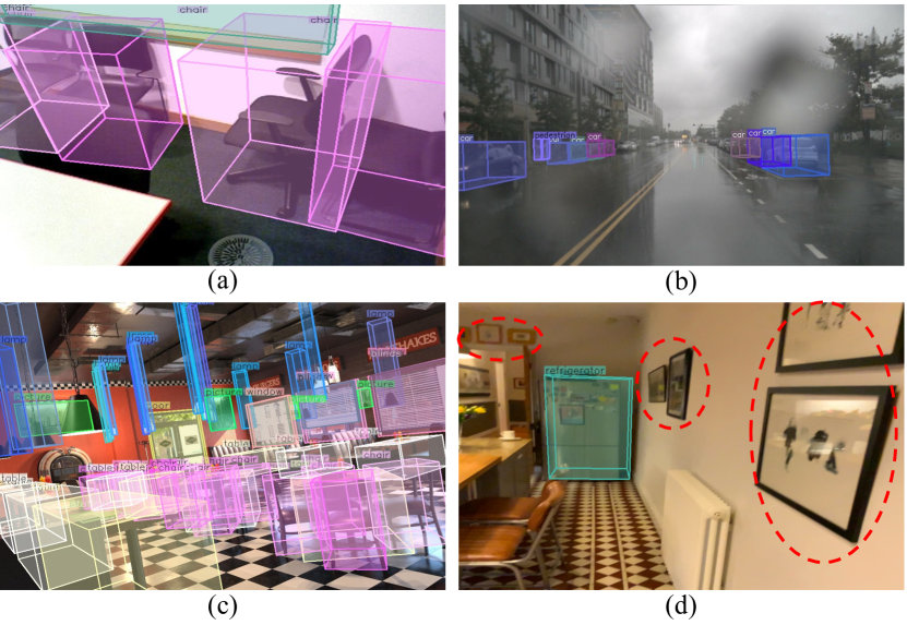
Figure 1: Illustration of some challenges (e.g., diverse geometry properties, heterogeneous domain distributions) in unified detection. (1) Comparing sub-figures (a) and (b), indoor objects are small and close, while outdoor objects are far and sparse. Besides, the camera parameters are highly varying. (2) Comparing sub-figures (a), (b), and (c), which correspond to a real-world indoor image, real-world outdoor image, and synthetic indoor image, the image styles are different. (3) Although the category “Picture” is labeled in sub-figure (c), it is not labeled in sub-figure (d), which suggests label conflict among different sub-datasets. Unlabeled objects are highlighted by red ellipses.

The most critical challenge in unified 3D object detection lies in addressing the distinct characteristics of different scenarios. For example, indoor objects are smaller and closer in proximity, while outdoor detection needs to cover a vast perception range. Recently, Cube RCNN [5] has served as a predecessor in studying this problem. It directly produces 3D box predictions in the camera view and adopts a depth decoupling strategy to tackle the domain gap among scenes. However, we observe it suffers serious convergence difficulty and is prone to collapsing during training.

To overcome the unstable convergence of Cube RCNN, we employ the recent popular bird’s-eye-view (BEV) detection paradigm to develop a unified 3D object detector. This is because the feature projection in the BEV paradigm aligns the image space with the 3D real-world space explicitly [15], which alleviates the learning ambiguity in monocular 3D object detection. Nevertheless, after extensive exploration, we find that naively adopting existing BEV detection architectures [15, 18] does not yield promising performance, which is mainly blamed on the following obstacles.

First of all, as shown in Fig. 1 (a) and (b), the geometry properties (e.g., perception ranges, target positions) between indoor and outdoor scenes are quite diverse. Specifically, indoor objects are typically a few meters away from the camera, while outdoor targets can be more than 100m away. Since a unified BEV detector is required to recognize objects in all scenarios, the BEV feature has to cover the maximum possible perception range. Meanwhile, as indoor objects are often small, the BEV grid resolution for indoor detection needs to be precise. All these characteristics can lead to unstable convergence and significant computational burden. To address these challenges, we develop a two-stage detection architecture. In this architecture, the first stage produces initial target position estimation, and the second stage locates targets using this estimation as prior information, which helps stabilize the convergence process. Moreover, we introduce an innovative uneven BEV grid split strategy that expands the BEV space range while maintaining a manageable BEV grid size. Furthermore, a sparse BEV feature projection strategy is developed to reduce the projection computational cost by 82.6%.

Another obstacle arises from the heterogeneous domain distributions (e.g., image styles, label definitions) across various scenarios. For example, as depicted in Fig. 1 (a), (b), and (c), the data can be collected in real scenes or synthesized virtually. Besides, comparing Fig. 1 (c) and (d), a class of objects may be annotated in a scene but not labeled in another scene, leading to confusion during network convergence. To handle these conflicts, we propose a unified domain alignment technique consisting of two parts, the domain adaptive layer normalization to align features, and the class alignment loss for alleviating label definition conflict.

Combining all these innovative techniques, a Unified Monocular Object DEtector named UniMODE is developed, and it achieves state-of-the-art (SOTA) performance on the Omni3D benchmark. In the unified detection setting, UniMODE surpasses the SOTA detector, Cube RCNN, by an impressive 4.9% in terms of $\rm AP_{3D}$ (average precision based on 3D intersection over union). Furthermore, when evaluated in indoor and outdoor detection settings individually, UniMODE outperforms Cube RCNN by 11.9% and 9.1%, respectively. This work represents a pioneering effort to explore the generalization of BEV detection architectures to unified detection, seamlessly integrating indoor and outdoor scenes. It showcases the immense potential of BEV detection across a broad spectrum of scenarios and underscores the versatility of this technology.

2 Related Work

Monocular 3D object detection. Due to its advantages of being economical and flexible, monocular 3D object detection grabs much research attention [22]. Existing detectors can be broadly categorized into two groups, camera-view detectors and BEV detectors. Among them, camera-view detectors generate results in the 2D image plane before converting them into the 3D real space [10, 25]. This group is generally easier to implement. However, the conversion from the 2D camera plane to 3D physical space can introduce additional errors [32], which negatively impact downstream planning tasks typically performed in 3D [7].

BEV detectors, on the other hand, transform image features from the 2D camera plane to the 3D physical space before generating results in 3D [12]. This approach benefits downstream tasks, as planning is also performed in the 3D space [18]. However, the challenge with BEV detectors is that the feature transformation process relies on accurate depth estimation, which can be difficult to achieve with only camera images [23]. As a result, convergence becomes unstable when dealing with diverse data scenarios [5].

Unified object detection. In order to improve the generalization ability of detectors, some works have explored the integration of multiple data sources during model training [34, 14]. For example, in the field of 2D object detection, SMD [40] improves the performance of detectors through learning a unified label space. In the 3D object detection domain, PPT [36] investigates the utilization of extensive 3D point cloud data from diverse datasets for pre-training detectors. In addition, Uni3DETR [35] reveals how to devise a unified point-based 3D object detector that behaves well in different domains. For the camera-based detection track, Cube RCNN [5] serves as the sole predecessor in the study of unified monocular 3D object detection. However, Cube RCNN is plagued by the unstable convergence issue, necessitating further in-depth analysis within this track.

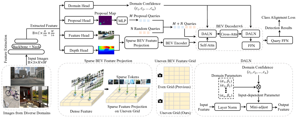
Figure 2: The overall detection framework of UniMODE. The illustrated modules proposed in this work include the proposal head, sparse BEV feature projection, uneven BEV feature grid, domain adaptive layer normalization, and class alignment loss.

3 Method

3.1 Overall Framework

The overall framework of UniMODE is illustrated in Fig. 2. As shown, a monocular image $I\in\mathbb{R}^{3\times H\times W}$ sampled from multiple scenarios (e.g., indoor and outdoor, real and synthetic, daytime and nighttime) are input to the feature extraction module (including a backbone and a neck) to produce representative feature $F\in\mathbb{R}^{C\times\frac{H}{16}\times\frac{W}{16}}$. Then, $F$ is processed by 4 fully convolutional heads, namely “domain head”, “proposal head”, “feature head”, and “depth head”, respectively. Among them, the role of the domain head is to predict which pre-defined data domain an input image is most relevant to, and the classification confidence produced by the domain head is subsequently utilized in domain alignment. The proposal head aims to estimate the rough target distribution before the 6 Transformer decoders, and the estimated distribution serves as prior information for the second-stage detection. This design alleviates the distribution mismatch between diverse training domains (refer to Section 3.2). The proposal head output is encoded as $M$ proposal queries. In addition, $N$ queries are randomly initialized and concatenated with the proposal queries for the second-stage detection, leading to $M+N$ queries in the second stage.

The feature head and depth head are responsible for projecting the image feature into the BEV plane and obtaining BEV feature. During this projection, we develop a technique to remove unnecessary projection points, which reduces the computing burden by about 82.6% (refer to Section 3.4). Besides, we propose the uneven BEV feature (refer to Section 3.3), which means the BEV grids closer to the camera enjoy more precise resolution, and the grids farther to the camera cover broader perception areas. This design well balances the grid size contradiction between indoor detection and outdoor detection without extra memory burden.

Obtaining the projected BEV feature, a BEV encoder is employed to further refine the feature, and 6 decoders are adopted to generate the second-stage detection results. As mentioned before, $M+N$ queries are used during this process. After the 6 decoders, the queries are decoded as detection results by querying the FFN. In the decoder part, the unified domain alignment strategy is devised to align the data of various scenarios via both the feature and loss perspectives. Refer to Section 3.5 for more details.

3.2 Two-Stage Detection Architecture

The integration of indoor and outdoor 3D object detection is challenging due to diverse geometry properties (e.g., perception ranges, target positions). Indoor detection typically involves close-range targets, while outdoor detection concerns targets scattered over a broader 3D space. As depicted in Fig. 3, the perception ranges and target positions in indoor and outdoor detection scenes vary significantly, which are challenging for traditional BEV 3D object detectors because of their fixed BEV feature resolutions.

The geometry property difference is identified as an essential reason causing the unstable convergence of BEV detectors [15]. For example, the target position distribution difference makes it challenging for Transformer-based detectors to learn how to update the query reference points gradually toward concerned objects. In fact, through visualization, we find the reference point updating in the 6 Transformer decoders is disordered. As a result, if we adopt the classical deformable DETR architecture [41] to build a 3D object detector, the training is easy to collapse due to the inaccurate positions of learned reference points, resulting in sudden gradient vanishing or exploding.

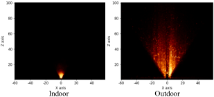
Figure 3: Indoor and outdoor target position distributions in the BEV space. The brighter a point shows, the more targets the corresponding BEV grid contains. The perception camera is located at the point with the coordinate $(0,0)$.

To overcome this challenge, we construct UniMODE in a two-stage detection fashion. In the first stage, we design a CenterNet [39] style head (the proposal head in Fig. 2) to produce detection proposals. Specifically, its predicted attributes include the 2D center Gaussion heatmap, offset from 2D centers to 3D centers, and 3D center depths of targets. The 3D center coordinates of proposals can be derived from these predicted attributes. Then, the proposals with top $M$ confidences are selected and encoded as $M$ proposal queries by an MLP layer. To account for any potential missed targets, another $N$ randomly initialized queries are concatenated with these proposal queries to perform information interaction in the 6 decoders of the second stage (the Transformer stage). In this way, the initial query reference points of the second detection stage are adjusted adaptively. Our experiments reveal that this two-stage architecture is essential for stable convergence.

Besides, since the positions of query reference points are not randomly initialized, the iterative bounding box refinement strategy proposed in deformable DETR [41] is abandoned as it may lead to a deterioration of reference points’ quality. In fact, we observe that this iterative bounding box refinement strategy could result in convergence collapse.

3.3 Uneven BEV Grid

A notable difference between indoor and outdoor 3D object detection lies in the geometry information (e.g., scale, proximity) of objects to the camera during data collection. Indoor environments typically feature smaller objects located closer to the camera, whereas outdoor environments involve larger objects positioned at greater distances. Furthermore, outdoor 3D object detectors must account for a wider perceptual range of the environment. Consequently, existing indoor 3D object detectors typically use smaller voxel or pillar sizes. For instance, the voxel size of CAGroup3D [31], a SOTA indoor 3D object detector, is 0.04 meters, and the maximum target depth in the SUN-RGBD dataset [29], a classic indoor dataset, is approximately 8 meters. In contrast, outdoor datasets exhibit much larger perception ranges. For example, the commonly used outdoor detection dataset KITTI [8] has a maximum depth range of 100 meters. Due to this vast perception range and limited computing resources, outdoor detectors employ larger BEV grid sizes, e.g. the BEV grid size in BEVDepth [11], a state-of-the-art outdoor 3D object detector, is 0.8 meters.

Therefore, the BEV grid sizes of current outdoor detectors are typically large to accommodate the vast perception range, while those of indoor detectors are small because of the intricate indoor scenes. However, since UniMODE aims to address both indoor and outdoor 3D object detection using a unified model structure and network weight, its BEV feature must cover a large perception area while still utilizing small BEV grids, which poses a massive challenge due to the limited GPU memory.

To overcome this challenge, we propose a solution that involves partitioning the BEV space into uneven grids, in contrast to the even grids utilized by existing detectors. As depicted in the bottom part of Fig. 2, we achieve this by employing a smaller size of grids closer to the camera and larger grids for those farther away. This approach enables UniMODE to effectively perceive a wide range of objects while maintaining small grid sizes for objects in close proximity. Importantly, this does not increase the total number of grids, thereby avoiding any additional computational burden. Specifically, assuming there are $N_{z}$ grids in the depth axis and the depth range is $(z_{min},z_{max})$, the grid size of the $i_{\rm th}$ grid $z_{i}$ is set to:

$$z_{i}=z_{min}+\frac{z_{max}-z_{min}}{N_{z}(N_{z}+1)}\cdot i(i+1).$$ (1)

Notably, the mathematical form in Eq. 1 is similar to the linear-increasing discretization of depth bin in CaDDN [26], while the essence is fundamentally different. In CaDDN, the feature projection distribution is adjusted to allocate more features to grids closer to the camera. In experiments, we observe that this adjustment results in a more imbalanced BEV feature, i.e., denser features in closer grids and more empty grids in farther grids. Since features in all grids are extracted by the same network, this imbalance degrades the performance. By contrast, our uneven BEV grid approach enhances detection precision by making the feature density more balanced.

3.4 Sparse BEV Feature Projection

The step of transforming the camera view feature into the BEV space is quite computationally expensive due to its numerous projection points. Specifically, considering the image feature $F_{i}\in\mathbb{R}^{C_{i}\times 1\times H_{f}\times W_{f}}$ and depth feature $F_{d}\in\mathbb{R}^{1\times C_{d}\times H_{f}\times W_{f}}$, the projection feature $F_{p}\in\mathbb{R}^{C_{i}\times C_{d}\times H_{f}\times W_{f}}$ is obtained by multiplying $F_{i}$ and $F_{d}$. Therefore, the projection point number $C_{i}\times C_{d}\times H_{f}\times W_{f}$ increases dramatically as the growth of $C_{d}$. The heavy computational burden of this feature projection step restricts the BEV feature resolution, and thus hinders unifying indoor and outdoor 3D object detection.

In this work, we observe that most projection points in $F_{p}$ are unnecessary because their values are quite tiny. This is essentially because of the small corresponding values in $F_{d}$, which imply that the model predicts there is no target in these specific BEV grids. Hence, the time spent on projecting features to these unconcerned grids can be saved.

Based on the above insights, we propose to remove the unnecessary projection points based on a pre-defined threshold $\tau$. Specifically, we eliminate the projection points in $F_{p}$ whose corresponding depth confidence of $F_{d}$ is smaller than $\tau$. In this way, most projection points are eliminated. For instance, when setting $\tau$ to 0.001, about 82.6% of projection points can be excluded.

3.5 Unified Domain Alignment

Heterogeneous domain distributions exist in diverse scenarios and we address this challenge via feature and loss views.

Domain adaptive layer normalization. For the feature view, we initialize domain-specific learnable parameters to address the variations observed in diverse training data domains. However, this strategy must adhere to two crucial requirements. Firstly, the detector should exhibit robust performance during inference, even when confronted with images from domains that are not encountered during training. Secondly, the introduction of these domain-specific parameters should incur minimal computational overhead.

Considering these two requirements, we propose the domain adaptive layer normalization (DALN) strategy. In this strategy, we first split the training data into $D$ domains. For the classic implementation of layer normalization (LN) [2], denoting the input sequence as $X_{l}\in\mathbb{R}^{B\times L\times C}$ and its element with the index $(b,l,c)$ as $x_{l}^{(b,l,c)}$, the corresponding output $\hat{x}_{l}^{(b,l,c)}$ of processing $x_{l}^{(b,l,c)}$ by LN is obtained as:

$$\hat{x}_{l}^{(b,l,c)}=\frac{x_{l}^{(b,l,c)}-\mu^{(b,l)}}{\sigma^{(b,l)}},$$ (2)

where

$$\mu^{(b,l)}=\frac{1}{C}\sum\limits_{i=1}^{C}x_{l}^{(b,l,i)},\sigma^{(b,l)}=\sqrt{\frac{1}{C}\sum\limits_{i=1}^{C}(x_{l}^{(b,l,c)}-\mu^{(b,l)})^{2}}.$$ (3)

In DALN, we build a set of learnable domain-specific parameters, i.e., $\{(\alpha_{i},\beta_{i})\}_{i=1}^{D}$, where $(\alpha_{i},\beta_{i})$ are the parameters corresponding to the $i_{\rm th}$ domain. $\{\alpha_{i}\}_{i=1}^{D}$ are initialized as 1 and $\{\beta_{i}\}_{i=1}^{D}$ are set to 0. Then, we establish a domain head consisting of several convolutional layers. As shown in Fig. 2, the domain head takes the feature $F$ as input and predicts the confidence scores that the input images $I$ belong to these $D$ domains. Denoting the confidence of the $b_{\rm th}$ image as $\{c_{i}\}_{i=1}^{D}$, the input-dependent parameters $(\alpha,\beta)$ are computed following:

$$\alpha=\sum\limits_{i=1}^{D}c_{i}\cdot\alpha_{i},\;\beta=\sum\limits_{i=1}^{D}c_{i}\cdot\beta_{i}.$$ (4)

Obtaining $(\alpha,\beta)$, we employ them to adjust the distribution of $\hat{x}_{l}^{(b,l,c)}$ with respect to $\bar{x}_{l}^{(b,l,c)}=\alpha\cdot\hat{x}_{l}^{(b,l,c)}+\beta$, where $\bar{x}_{l}^{(b,l,c)}$ denotes the updated distribution. In this way, the feature distribution in UniMODE can be adjusted according to input images self-adaptively, and the increased parameters are negligible. Additionally, when an image unseen in the training set is input, DALN still works well, because the unseen image can still be classified as a weighted combination of these $D$ domains.

Although there exist a few previous techniques related to adaptive normalization, almost all of them are based on regressing input-dependent parameters directly [36]. So, they need to build a special regression head for every normalization layer. By contrast, DALN enables all layers to share the same domain head, so the computing burden is much smaller. Besides, DALN introduces domain-specific parameters, which are more stable to train.

Class alignment loss. In the loss view, we aim to address the heterogeneous label conflict when combining multiple data sources. Specifically, there are 6 independently labeled sub-datasets in Omni3D, and their label spaces are different. For example, as presented in Fig. 4, although the Window class is annotated in ARKitScenes, while it is not labeled in Hypersim. As the label space of Omni3D is the union of all classes in all subsets, the unlabeled window in Fig. 4 (a) becomes a missing target that harms convergence stability.

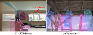
Figure 4: An example of heterogeneous label conflict among sub-datasets in Omni3D. As shown, “Window” is not labeled in ARKitScenes while labeled in Hypersim, so the unlabeled window in (a) could harm the convergence stability of detectors.

The two-stage detection architecture described in Section 3.2 can alleviate the aforementioned problem to some extent, because it helps the detector concentrate on foreground objects, and the unlabeled objects are overlooked to compute loss. To address this problem further, we devise a simple strategy, the class alignment loss. Specifically, denoting the label space of the $i_{\rm th}$ dataset as $\Omega_{i}$, we compute loss on the $i_{\rm th}$ dataset as:

$$L_{i}=\{\begin{array}[]{lcl}\gamma\cdot l(y,\bar{y}),(\bar{y}\notin\Omega_{i})\wedge(\bar{y}=\mathcal{B})\\ l(y,\bar{y}),others\\ \end{array},$$ (7)

where $l(\cdot)$, $y$, $\bar{y}$, $\mathcal{B}$ are the loss function, class prediction, class label, and background class, respectively. $\gamma$ is a factor for reducing the punishment to classes not included in the label space of this sample.

Method	OMNI3D_OUT			OMNI3D_IN		OMNI3D
	${\rm AP^{kit}_{3D}}\uparrow$	${\rm AP^{nus}_{3D}}\uparrow$	${\rm AP^{out}_{3D}}\uparrow$	${\rm AP^{sun}_{3D}}\uparrow$	${\rm AP^{in}_{3D}}\uparrow$	${\rm AP_{3D}^{25}}\uparrow$	${\rm AP_{3D}^{50}}\uparrow$	${\rm AP_{3D}^{near}}\uparrow$	${\rm AP_{3D}^{med}}\uparrow$	${\rm AP_{3D}^{far}}\uparrow$	${\rm AP_{3D}}\uparrow$
M3D-RPN [4]	10.4%	17.9%	13.7%	-	-	-	-	-	-	-	-
SMOKE [19]	25.4%	20.4%	19.5%	-	-	-	-	-	-	-	9.6%
FCOS3D [32]	14.6%	20.9%	17.6%	-	-	-	-	-	-	-	9.8%
PGD [33]	21.4%	26.3%	22.9%	-	-	-	-	-	-	-	11.2%
GUPNet [21]	24.5%	20.5%	19.9%	-	-	-	-	-	-	-	-
ImVoxelNet [28]	23.5%	23.4%	21.5%	30.6%	-	-	-	-	-	-	9.4%
BEVFormer [15]	23.9%	29.6%	25.9%	-	-	2718	2718	2718	2718	2718	2718
PETR [18]	30.2%	30.1%	27.8%	-	-	2718	2718	2718	2718	2718	2718
Cube RCNN [5]	36.0%	32.7%	31.9%	36.2%	15.0%	24.9%	9.5%	27.9%	12.1%	8.5%	23.3%
UniMODE	40.2%	40.0%	39.1%	36.1%	22.3%	28.3%	7.4%	29.7%	12.7%	8.1%	25.5%
UniMODE*	41.3%	43.6%	41.0%	39.8%	26.9%	30.2%	10.6%	31.1%	14.9%	8.7%	28.2%

Table 1: Performance comparison between the proposed UniMODE and other 3D object detectors. In the $2_{\rm nd}\sim 4_{\rm th}$ columns, the detectors are trained using KITTI and nuScenes. These three columns reflect the detection precision on KITTI, nuScenes, and overall outdoor detection performance, respectively. The $5_{\rm th}\sim 6_{\rm th}$ columns correspond to indoor detection results. Among them, the $5_{\rm th}$ column is the performance that detectors are trained and validated on SUN-RGBD. In the $6_{\rm th}$ column, detectors are trained and evaluated by combining SUN-RGBD, ARKitScenes, and Hypersim. The $7_{\rm th}\sim 12_{\rm th}$ columns represent the overall detection performance where detectors are trained and validated utilizing all data in Omni3D. UniMODE and UniMODE* denote the proposed detectors, taking DLA34 and ConvNext-Base as the backbones, respectively. The best results given various metrics are marked in bold. The “2718” means that the model does not converge well, and the obtained performance is quite poor. The “-” means this result is reported in previous literature.

Backbone	$\rm AP_{3D}^{sun}\uparrow$	$\rm AP_{3D}^{hyp}\uparrow$	$\rm AP_{3D}^{ark}\uparrow$	$\rm AP_{3D}^{obj}\uparrow$	$\rm AP_{3D}^{kit}\uparrow$	$\rm AP_{3D}^{nus}\uparrow$
DLA34	21.0%	6.7%	42.3%	52.5%	27.8%	31.7%
ConvNext	23.0%	8.1%	48.0%	66.1%	29.2%	36.0%

Table 2: Detailed performance of UniMODE on various sub-datasets in Omni3D. The detectors are trained and evaluated using the whole Omni3D training and testing data. The results of adopting two different backbones are presented.

4 Experiment

Implementation details. The perception ranges in the X-axis, Y-axis, and Z-axis of the camera coordinate system are $(-30,30)$, $(-40,40)$, $(0,80)$ meters, respectively. If without a special statement, the BEV grid resolution is $(60,80)$. The factor $\gamma$ defined in the class alignment loss is set to 0.2. $M$ and $N$ are set to 100. The adopted optimizer is AdamW, and the learning rate is set to $12e^{-4}$ for a batch size of 192. The experiments are primarily conducted on 4 A100 GPUs. The total loss includes two parts, the proposal head loss and the query FFN loss. The proposal head loss consists of the heatmap classification loss and depth regression loss. The query FFN loss comprises the classification loss (a cross-entropy loss) and regression loss ($L_{1}$ loss for predicting 3D center, dimension, and orientation). The total loss is the weighted sum of these loss items. No special loss is set for the $M$ proposal query generation.

Dataset. The experiments in this section are performed on Omni3D, the sole large-scale 3D object detection benchmark encompassing both indoor and outdoor scenes. Omni3D is built upon six well-known datasets including KITTI [8], SUN-RGBD [29], ARKitScenes [3], Objectron [1], nuScenes [6], and Hypersim [27]. Among these datasets, KITTI and nuScenes focus on urban driving scenes, which are real-world outdoor scenarios. SUN-RGBD, ARKitScenes, and Objectron primarily pertain to real-world indoor environments. Compared with outdoor datasets, the required perception ranges of indoor datasets are smaller and the object categories are more diverse. Hypersim, distinct from the aforementioned five datasets, is a virtually synthesized dataset. Thus, Hypersim allows for the annotation of object classes that are challenging to label in real scenes, such as transparent objects (e.g., windows) and very thin objects (e.g., carpets). The Omni3D dataset comprises a total of 98 object categories and 3 million 3D box annotations, spanning 234,000 images. The evaluation metric is $\rm AP_{3D}$, which reflects the 3D Intersection over Union (IoU) between 3D box prediction and label.

Experimental settings. As Omni3D is a large-scale dataset, training models on it necessitates many GPUs. For example, the authors of Cube RCNN run each experiment with 48 V100s for 4$\sim$5 days. In this work, the experiments in Section 4.1 are performed in the high computing resource setting (the input image resolution is $1280\times 1024$, the backbone is ConvNext-Base [20], all training data). Since our computing resources are limited, unless explicitly stated otherwise, the remaining experiments are conducted in the low computing resource setting (the input resolution is $640\times 512$, the backbone is DLA34 [37], fixed 20% of all training data sampled from all 6 sub-datasets).

4.1 Performance Comparison

In this part, we compare the performance of the proposed detector with previous methods. Among them, Cube RCNN is the sole detector that also explores unified detection. BEVFormer [15] and PETR [18] are two popular BEV detectors, and we reimplement them in the Omni3D benchmark to get the detection scores. The performance of the other compared detectors is obtained from [5]. All the results are given in Table 1. In addition, we present the detailed detection scores of UniMODE on various sub-datasets in Omni3D as Table 2.

According to the results, we can observe that UniMODE achieves the best results in all metrics. It surpasses the SOTA Cube RCNN by 4.9% given the primary metric $\rm AP_{3D}$. Besides DLA34, we also try another backbone ConvNext-Base. This is because previous papers suggest that DLA34 is commonly used in camera-view detectors like Cube RCNN but not suitable for BEV detectors [13]. Since UniMODE is a BEV detector, only testing the performance of UniMODE with DLA34 is unfair. Thus, we also test the UniMODE with ConvNext-Base, and the result suggests that the performance is boosted significantly. Additionally, the speed of UniMODE is also promising. Test on 1 A100 GPU, the inference speeds of UniMODE under the high and low computing resource settings are 21.41 FPS and 43.48 FPS separately.

In addition, it can be observed from Table 1 that BEVFormer and PETR do not converge well in the unified detection setting while behaving promisingly trained with outdoor datasets. This phenomenon implies the difficulty of unifying indoor and outdoor 3D object detection. Through analysis, we find that BEVFormer obtains poor results when using data of all domains because its convergence is quite unstable, and the loss curve often boosts to a high value during training. PETR does not behave well since it implicitly learns the correspondence relation between 2D pixels and 3D voxels. When the camera parameters keep similar across all samples in a dataset like nuScenes [6], PETR converges smoothly. Nevertheless, when trained in a dataset with dramatically changing camera parameters like Omni3D, PETR becomes much more difficult to train.

4.2 Ablation Studies

PH	UBG	SBFP	UDA	$\rm AP_{3D}^{in}\uparrow$	$\rm AP_{3D}^{out}\uparrow$	$\rm AP_{3D}\uparrow$	Improvement
				10.9%	14.3%	12.3%	-
✓				13.4%	22.2%	15.9%	3.6%$\uparrow$
✓	✓			14.00%	23.8%	16.6%	0.7%$\uparrow$
✓	✓	✓		13.4%	23.7%	16.6%	0.0$\%\uparrow$
✓	✓	✓	✓	14.8%	24.5%	17.4%	0.8%$\uparrow$

Table 3: Ablation study on proposed strategies, which verify the effects of proposal head (PH), uneven BEV grid (UBG), sparse BEV feature projection(SBFP), and unified domain alignment (UDA). The last column presents the improvement of each row compared with the top row. $\rm AP_{3D}^{in}$ and $\rm AP_{3D}^{out}$ reflect the indoor and outdoor detection performance, respectively. Notably, although SBFP does not boost the detection precision, it reduces the computational cost of the BEV feature projection by 82.6%.

Key component designs. We ablate the effectiveness of the proposed strategies in UniMODE, including proposal head, uneven BEV grid, sparse BEV feature projection, and unified domain alignment. The experimental results are presented in Table 3. Notably, as mentioned before, the experiments in this part are conducted in the low computing resource setting due to the limited computing resources.

According to the results in Table 3, we can observe that all these strategies are very effective. Among them, the proposal head boosts the result by the most significant margin. Specifically, the proposal head enhances the overall detection performance metric $\rm AP_{3D}$ by 3.6%. Meanwhile, the indoor and outdoor detection metrics $\rm AP_{3D}^{in}$ and $\rm AP_{3D}^{out}$ are boosted by 2.5% and 7.9% separately. As discussed in Section 3.2, the proposal head is quite effective because it stabilizes the convergence process of UniMODE and thus favors detection accuracy. The collapse does not happen after using the proposal head. In addition, although the sparse BEV feature projection strategy does not improve the detection precision, it reduces the projection cost by 82.6%.

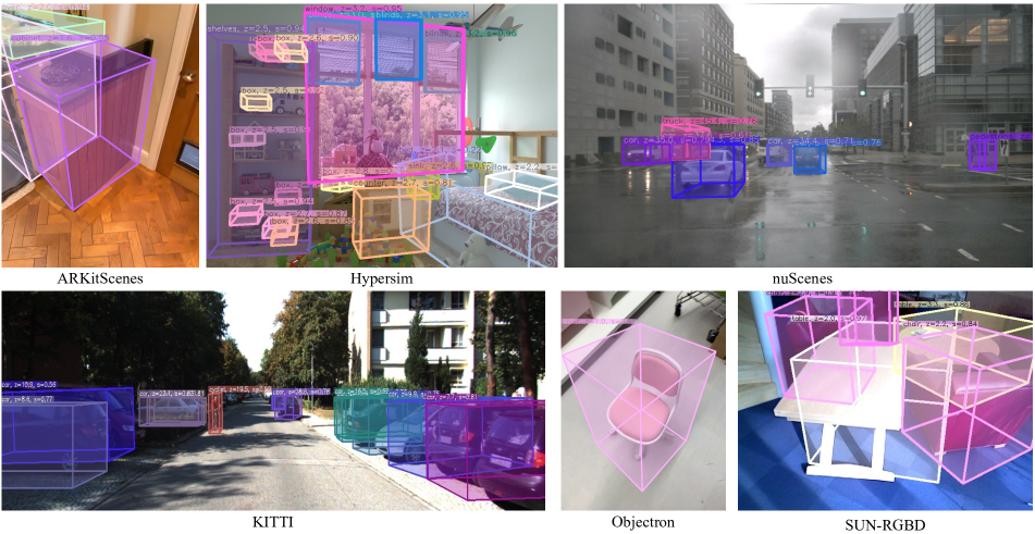
Figure 5: Visualization of detection results on various sub-datasets in Omni3D.

Grid Size (m)	Depth Bin	$\rm AP_{3D}^{in}\uparrow$	$\rm AP_{3D}^{out}\uparrow$	$\rm AP_{3D}\uparrow$
1	Even	14.8%	24.5%	17.4%
1	Uneven	12.1%	22.6%	15.3%
0.5	Even	15.4%	25.5%	18.1%
2	Even	14.0%	23.9%	16.5%

Table 4: Ablation study on grid size and depth bin split strategy in uneven BEV grid.

$\tau$	Remove Ratio (%)	$\rm AP_{3D}^{in}\uparrow$	$\rm AP_{3D}^{out}\uparrow$	$\rm AP_{3D}\uparrow$
0	0.0	14.9%	24.7%	17.4%
1e-3	82.6	14.8%	24.5%	17.4%
1e-2	94.3	12.1%	21.9%	15.0%
1e-1	98.3	4.7%	3.6%	4.7%

Table 5: Ablation study on $\tau$ in sparse BEV feature projection.

Uneven BEV grid. We study the effect of BEV feature grid size and depth bin split strategy in uneven BEV grid design, and the results are presented in Table 4. When the depth bin split is uneven, we split the depth bin range following Eq. 1.

Comparing the $1_{\rm st}$ and $2_{\rm nd}$ rows of results in Table 4, we can find that uneven depth bin deteriorates detection performance. We speculate this is because this strategy projects more points in closer BEV grids while fewer points in farther grids, which further increases the imbalanced distribution of projection features. Additionally, comparing the $1_{\rm st}$, $3_{\rm rd}$, and $4_{\rm th}$ rows of results in Table 4, it is observed that smaller BEV grids lead to better performance. We set the BEV grid size to 1m rather than 0.5m in all the other experiments due to limited computing resources and the vast training data volume of Omni3D, i.e., if we decrease the size of BEV grids, the performance of UniMODE can be further boosted compared with the current performance.

Sparse BEV feature projection. As mentioned in Section 3.4, the BEV feature projection process is computationally expensive. To reduce this cost, we propose to remove unimportant projection points. Although this strategy enhances network efficiency significantly, it could deteriorate detection accuracy and convergence stability, which is exactly a trade-off. In this part, we study this trade-off through experiments. Specifically, as introduced in Section 3.4, we remove unimportant projection points based on a pre-defined hyper-parameter $\tau$. The value of $\tau$ is adjusted to analyze how the removed projection point ratio affects performance. The results are reported in Table 5.

It can be observed from Table 5 that when $\tau$ is 0, which means no feature is discarded, the best performance across all rows is arrived. When we set $\tau$ to $1e^{-3}$, about 82.6% of the feature is discarded while the performance of the detector remains very similar to the one with $\tau=0$. This phenomenon suggests that the discarded feature is unimportant for final detection accuracy. Then, when we increase $\tau$ to $1e^{-2}$ and $1e^{-1}$, we can find that the corresponding performances drop dramatically. This observation indicates that when we discard superfluous features, the detection precision and even training stability are influenced significantly. Combining all the observations, we set $\tau$ to $1e^{-3}$ and drop $82.6\%$ of unimportant feature in UniMODE, which reduces the computational cost by $82.6\%$ while maintaining similar performance as the one without dropping features.

Effectiveness of DALN. In this experiment, we validate the effectiveness of DALN through comparing the performances of the naive baseline without any domain adaptive strategy, the baseline predicting dynamic parameters with direct regression (DR) [24], and the baseline with DALN (our proposed). All these models are trained using only ARKitScenes and evaluated with ARKitScenes (in-domain) and SUN-RGBD (out-of-domain) separately. The result is presented in Table 6. It can be observed that DR could degrade the detection accuracy while DALN boosts the performance significantly, which reveals the zero-shot out-of-domain effectiveness of DALN.

Method	None		DR		DALN
	${\rm AP^{ark}_{3D}}\uparrow$	${\rm AP^{sun}_{3D}}\uparrow$	${\rm AP^{ark}_{3D}}\uparrow$	${\rm AP^{sun}_{3D}}\uparrow$	${\rm AP^{ark}_{3D}}\uparrow$	${\rm AP^{sun}_{3D}}\uparrow$
Result	33.6%	12.3%	33.9%	12.1%	35.0%	13.0%

Table 6: Analysis on the effectiveness of DALN.

4.3 Cross-domain Evaluation

We evaluate the generalization ability of UniMODE in this part by conducting the cross-domain evaluation. Specifically, we train a detector on a sub-dataset in Omni3D and test the performance of this detector on different other sub-datasets. The experiments are conducted in two settings. In the zero-shot setting, the test domain is completely unseen. In the $\delta$-tune setting, 1% of training set data from the test domain is used to fine-tune the Query FFN in UniMODE for 1 epoch. The experimental results are presented in Table 7.

Train	Zero-Shot			$\delta$-Tune
	$\rm AP_{3D}^{hyp}\uparrow$	$\rm AP_{3D}^{sun}\uparrow$	$\rm AP_{3D}^{ark}\uparrow$	$\rm AP_{3D}^{hyp}\uparrow$	$\rm AP_{3D}^{sun}\uparrow$	$\rm AP_{3D}^{ark}\uparrow$
Hypersim	14.7%	5.6%	3.6%	14.7%	18.5%	18.9%
SUN-RGBD	3.0%	28.5%	8.8%	7.5%	28.5%	27.2%
ARKitScenes	4.2%	13.0%	35.0%	10.4%	22.8%	35.0%

Table 7: Cross-domain evaluation in indoor sub-datasets. In this experiment, the detector is first trained in a domain and tested on other domains in two settings, zero-shot and $\delta$-tune.

According to the results in the $2_{\rm st}\sim 4_{\rm th}$ columns of Table 7, we can find that when a detector is trained and validated in the same indoor sub-dataset, its performance is promising. However, when evaluated on another completely unseen sub-dataset, the accuracy is limited. This is partly because monocular 3D depth estimation is an ill-posed problem. When the training and validation data belong to differing domains, predicting depth accurately is challenging, especially for the virtual dataset Hypersim.

Then, we introduce another testing setting, $\delta$-tuning. In this setting, if a detector is tested on another domain different from the train domain, the Query FFN is fine-tuned by 1% of training data from the test domain. The results of this $\delta$-tuning setting are reported in the $5_{\rm st}\sim 7_{\rm th}$ columns of Table 7. We can observe that when fine-tuned with only a handful of data, the performance of UniMODE becomes much more promising. This result suggests that the superiority of UniMODE in serving as a foundational model. It can benefit practical applications by only incorporating a little training data from the test domain.

4.4 Visualization

We visualize the detection results of UniMODE on various sub-datasets in Omni3D. The illustrated results are shown in Fig. 5, where UniMODE performs quite well on all the data samples, and accurately captures the 3D object bounding boxes under both complex indoor and outdoor scenarios.

Besides, as mentioned before, training instability is the primary challenge in unifying diverse training domains. To explain the meaning of training instability more clearly, we present the loss curves of UniMODE and an unstable case of PETR in Fig. 6. It can be found that there exists sudden loss boost and continuous gradient collapse in the training of PETR, while UniMODE converges smoothly.

Figure 6: The trainings loss curves of UniMODE and PETR.

5 Conclusion and Limitation

In this work, we have proposed a unified monocular 3D object detector named UniMODE, which contains several well-designed techniques to address many challenges observed in unified 3D object detection. The proposed detector has achieved SOTA performance on the Omni3D benchmark and presented high efficiency. Extensive experiments are conducted to verify the effectiveness of the proposed techniques. The limitation of the detector is its zero-shot generalization ability on unseen data scenarios is still limited. In the future, we will continue to study how to boost the zero-shot generalization ability of UniMODE through strategies like scaling up the training data.

References

- Ahmadyan et al. [2021] Adel Ahmadyan, Liangkai Zhang, Artsiom Ablavatski, Jianing Wei, and Matthias Grundmann. Objectron: A large scale dataset of object-centric videos in the wild with pose annotations. In CVPR, pages 7822–7831, 2021.
- Ba et al. [2016] Jimmy Lei Ba, Jamie Ryan Kiros, and Geoffrey E Hinton. Layer normalization. arXiv preprint arXiv:1607.06450, 2016.
- Baruch et al. [2021] Gilad Baruch, Zhuoyuan Chen, Afshin Dehghan, Yuri Feigin, Peter Fu, Thomas Gebauer, Daniel Kurz, Tal Dimry, Brandon Joffe, Arik Schwartz, et al. Arkitscenes: A diverse real-world dataset for 3d indoor scene understanding using mobile rgb-d data. In NeurIPS, 2021.
- Brazil and Liu [2019] Garrick Brazil and Xiaoming Liu. M3d-rpn: Monocular 3d region proposal network for object detection. In ICCV, pages 9287–9296, 2019.
- Brazil et al. [2023] Garrick Brazil, Abhinav Kumar, Julian Straub, Nikhila Ravi, Justin Johnson, and Georgia Gkioxari. Omni3d: A large benchmark and model for 3d object detection in the wild. In CVPR, pages 13154–13164, 2023.
- Caesar et al. [2020] Holger Caesar, Varun Bankiti, Alex H Lang, Sourabh Vora, Venice Erin Liong, Qiang Xu, Anush Krishnan, Yu Pan, Giancarlo Baldan, and Oscar Beijbom. nuscenes: A multimodal dataset for autonomous driving. In CVPR, pages 11621–11631, 2020.
- Claussmann et al. [2019] Laurene Claussmann, Marc Revilloud, Dominique Gruyer, and Sébastien Glaser. A review of motion planning for highway autonomous driving. IEEE Transactions on Intelligent Transportation Systems, 21(5):1826–1848, 2019.
- Geiger et al. [2012] Andreas Geiger, Philip Lenz, and Raquel Urtasun. Are we ready for autonomous driving? the kitti vision benchmark suite. In CVPR, pages 3354–3361, 2012.
- Li and Zhao [2021] Peixuan Li and Huaici Zhao. Monocular 3d detection with geometric constraint embedding and semi-supervised training. IEEE Robotics and Automation Letters, 6(3):5565–5572, 2021.
- Li et al. [2022a] Yingyan Li, Yuntao Chen, Jiawei He, and Zhaoxiang Zhang. Densely constrained depth estimator for monocular 3d object detection. In ECCV, pages 718–734, 2022a.
- Li et al. [2023a] Yinhao Li, Zheng Ge, Guanyi Yu, Jinrong Yang, Zengran Wang, Yukang Shi, Jianjian Sun, and Zeming Li. Bevdepth: Acquisition of reliable depth for multi-view 3d object detection. In AAAI, pages 1477–1485, 2023a.
- Li et al. [2023b] Yinhao Li, Zheng Ge, Guanyi Yu, Jinrong Yang, Zengran Wang, Yukang Shi, Jianjian Sun, and Zeming Li. Bevdepth: Acquisition of reliable depth for multi-view 3d object detection. In AAAI, pages 1477–1485, 2023b.
- Li et al. [2022b] Zhuoling Li, Zhan Qu, Yang Zhou, Jianzhuang Liu, Haoqian Wang, and Lihui Jiang. Diversity matters: Fully exploiting depth clues for reliable monocular 3d object detection. In CVPR, pages 2791–2800, 2022b.
- Li et al. [2022c] Zhuoling Li, Haohan Wang, Tymosteusz Swistek, En Yu, and Haoqian Wang. Efficient few-shot classification via contrastive pre-training on web data. IEEE Transactions on Artificial Intelligence, 2022c.
- Li et al. [2022d] Zhiqi Li, Wenhai Wang, Hongyang Li, Enze Xie, Chonghao Sima, Tong Lu, Yu Qiao, and Jifeng Dai. Bevformer: Learning bird’s-eye-view representation from multi-camera images via spatiotemporal transformers. In ECCV, pages 1–18, 2022d.
- Li et al. [2023c] Zhuoling Li, Chunrui Han, Zheng Ge, Jinrong Yang, En Yu, Haoqian Wang, Hengshuang Zhao, and Xiangyu Zhang. Grouplane: End-to-end 3d lane detection with channel-wise grouping. arXiv preprint arXiv:2307.09472, 2023c.
- Li et al. [2023d] Zhuoling Li, Chuanrui Zhang, Wei-Chiu Ma, Yipin Zhou, Linyan Huang, Haoqian Wang, SerNam Lim, and Hengshuang Zhao. Voxelformer: Bird’s-eye-view feature generation based on dual-view attention for multi-view 3d object detection. arXiv preprint arXiv:2304.01054, 2023d.
- Liu et al. [2022a] Yingfei Liu, Tiancai Wang, Xiangyu Zhang, and Jian Sun. Petr: Position embedding transformation for multi-view 3d object detection. In ECCV, pages 531–548, 2022a.
- Liu et al. [2020] Zechen Liu, Zizhang Wu, and Roland Tóth. Smoke: Single-stage monocular 3d object detection via keypoint estimation. In CVPR Workshops, pages 996–997, 2020.
- Liu et al. [2022b] Zhuang Liu, Hanzi Mao, Chao-Yuan Wu, Christoph Feichtenhofer, Trevor Darrell, and Saining Xie. A convnet for the 2020s. In CVPR, pages 11976–11986, 2022b.
- Lu et al. [2021] Yan Lu, Xinzhu Ma, Lei Yang, Tianzhu Zhang, Yating Liu, Qi Chu, Junjie Yan, and Wanli Ouyang. Geometry uncertainty projection network for monocular 3d object detection. In ICCV, pages 3111–3121, 2021.
- Mao et al. [2022] Jiageng Mao, Shaoshuai Shi, Xiaogang Wang, and Hongsheng Li. 3d object detection for autonomous driving: A review and new outlooks. arXiv preprint arXiv:2206.09474, 2022.
- Park et al. [2021] Dennis Park, Rares Ambrus, Vitor Guizilini, Jie Li, and Adrien Gaidon. Is pseudo-lidar needed for monocular 3d object detection? In ICCV, pages 3142–3152, 2021.
- Park et al. [2019] Taesung Park, Ming-Yu Liu, Ting-Chun Wang, and Jun-Yan Zhu. Semantic image synthesis with spatially-adaptive normalization. In CVPR, pages 2337–2346, 2019.
- Peng et al. [2022] Liang Peng, Xiaopei Wu, Zheng Yang, Haifeng Liu, and Deng Cai. Did-m3d: Decoupling instance depth for monocular 3d object detection. In ECCV, pages 71–88, 2022.
- Reading et al. [2021] Cody Reading, Ali Harakeh, Julia Chae, and Steven L Waslander. Categorical depth distribution network for monocular 3d object detection. In CVPR, pages 8555–8564, 2021.
- Roberts et al. [2021] Mike Roberts, Jason Ramapuram, Anurag Ranjan, Atulit Kumar, Miguel Angel Bautista, Nathan Paczan, Russ Webb, and Joshua M Susskind. Hypersim: A photorealistic synthetic dataset for holistic indoor scene understanding. In ICCV, pages 10912–10922, 2021.
- Rukhovich et al. [2022] Danila Rukhovich, Anna Vorontsova, and Anton Konushin. Imvoxelnet: Image to voxels projection for monocular and multi-view general-purpose 3d object detection. In WACV, pages 2397–2406, 2022.
- Song et al. [2015] Shuran Song, Samuel P Lichtenberg, and Jianxiong Xiao. Sun rgb-d: A rgb-d scene understanding benchmark suite. In CVPR, pages 567–576, 2015.
- Tellex et al. [2011] Stefanie Tellex, Thomas Kollar, Steven Dickerson, Matthew Walter, Ashis Banerjee, Seth Teller, and Nicholas Roy. Understanding natural language commands for robotic navigation and mobile manipulation. In AAAI, pages 1507–1514, 2011.
- Wang et al. [2022a] Haiyang Wang, Shaocong Dong, Shaoshuai Shi, Aoxue Li, Jianan Li, Zhenguo Li, Liwei Wang, et al. Cagroup3d: Class-aware grouping for 3d object detection on point clouds. NeurIPS, 35:29975–29988, 2022a.
- Wang et al. [2021] Tai Wang, Xinge Zhu, Jiangmiao Pang, and Dahua Lin. Fcos3d: Fully convolutional one-stage monocular 3d object detection. In ICCV, pages 913–922, 2021.
- Wang et al. [2022b] Tai Wang, ZHU Xinge, Jiangmiao Pang, and Dahua Lin. Probabilistic and geometric depth: Detecting objects in perspective. In CoRL, pages 1475–1485, 2022b.
- Wang et al. [2019] Xudong Wang, Zhaowei Cai, Dashan Gao, and Nuno Vasconcelos. Towards universal object detection by domain attention. In CVPR, pages 7289–7298, 2019.
- Wang et al. [2023] Zhenyu Wang, Ya-Li Li, Xi Chen, Hengshuang Zhao, and Shengjin Wang. Uni3detr: Unified 3d detection transformer. In NeurIPS, 2023.
- Wu et al. [2023] Xiaoyang Wu, Zhuotao Tian, Xin Wen, Bohao Peng, Xihui Liu, Kaicheng Yu, and Hengshuang Zhao. Towards large-scale 3d representation learning with multi-dataset point prompt training. arXiv preprint arXiv:2308.09718, 2023.
- Yu et al. [2018] Fisher Yu, Dequan Wang, Evan Shelhamer, and Trevor Darrell. Deep layer aggregation. In CVPR, pages 2403–2412, 2018.
- Zhang et al. [2021] Yunpeng Zhang, Jiwen Lu, and Jie Zhou. Objects are different: Flexible monocular 3d object detection. In CVPR, pages 3289–3298, 2021.
- Zhou et al. [2019] Xingyi Zhou, Dequan Wang, and Philipp Krähenbühl. Objects as points. arXiv preprint arXiv:1904.07850, 2019.
- Zhou et al. [2022] Xingyi Zhou, Vladlen Koltun, and Philipp Krähenbühl. Simple multi-dataset detection. In CVPR, pages 7571–7580, 2022.
- Zhu et al. [2020] Xizhou Zhu, Weijie Su, Lewei Lu, Bin Li, Xiaogang Wang, and Jifeng Dai. Deformable detr: Deformable transformers for end-to-end object detection. In ICLR, 2020.