A New Probe of Cosmic Birefringence Using Galaxy Polarization and Shapes

Abstract

We propose a new method to search for parity-violating new physics via measurements of cosmic birefringence and demonstrate its power in detecting the topological effect originating from an axion string network with an axion-photon coupling as a motivated source of cosmic birefringence. The method, using large galaxy samples, exploits an empirical correlation between the polarization direction of the integrated radio emission from a spiral galaxy and its apparent shape. We devise unbiased minimum-variance quadratic estimators for discrete samples of galaxies with both integrated radio polarization and shape measurements. Assuming a synergy with overlapping optical imaging surveys, we forecast the sensitivity to polarization rotation of the forthcoming SKA radio continuum surveys of spiral galaxies out to $z\sim 1.5$. The angular noise power spectrum of polarization rotation using our method can be lower than that expected from CMB Stage-IV experiments, when assuming a wide survey covering $\sim 1000\,{\rm deg}^{2}$ and reaching an RMS flux of $\sim 1\,\mu{\rm Jy}$. Our method will be complementary to CMB-based methods as it will be subject to different systematics. It can be generalized to probe time-varying or redshift-varying birefringence signals.

Introduction — The question of whether discrete transformations—charge conjugation (C), parity (P), and time reversal (T)—are fundamental symmetries of the Universe has led to important discoveries [1, 2, 3]. The axion was originally proposed to solve the strong CP problem in Quantum Chromodynamics [4, 5, 6, 7]. More recently, generic axions are shown to arise abundantly in string theory [8, 9]. The Chern-Simons interaction between the axion and electromagnetism leads to the parity-violating cosmic birefringence effect [10]:

$$\mathcal{L}=-\frac{1}{4}\,g_{a\gamma\gamma}\,a\,F^{\mu\nu}\,\tilde{F}_{\mu\nu}=g_{a\gamma\gamma}\,a\,{\bf E}\cdot{\bf B},$$ (1)

where $a$ is the axion field, $F^{\mu\nu}$ is the electromagnetic field strength tensor, and $\tilde{F}^{\mu\nu}\equiv(1/2)\,\epsilon_{\mu\nu\rho\sigma}\,F^{\rho\sigma}$ is its dual. As a photon travels through a background axion field, its plane of polarization rotates by an angle proportional to the net change in the axion field value along the photon’s worldline, multiplied by the axion-photon coupling constant $g_{a\gamma\gamma}$. The rotation is independent of the photon’s frequency due to the topological nature of the interaction [11, 12, 13]. Recent analyses of the cosmic microwave background (CMB) have shown hints of a rotation of its polarization anisotropies that is highly coherent across the sky, on the order of a fraction of a degree [14, 15]. Possible contamination from foregrounds is being investigated [16]. On the other hand, searches for anisotropic birefrigence have not so far uncovered a signal [17, 18, 19, 20].

Measuring birefringence toward any single astrophysical source or along any single sightline is hindered by our lack of knowledge about the intrinsic polarization direction of the source. When the CMB is used as the probe, this fundamental problem is solved statistically. Rotation angles that are correlated across the sky are measurable owing to the state-of-the-art cosmological model that accurately predicts the Gaussian statistics of the primary CMB polarization anisotropies [21, 22, 23, 20]. To confidently confirm a signal of cosmic birefringence, it is important to consider alternative methods of detection based on distinct cosmological or astrophysical probes whose systematics are independent of CMB measurements.

In this paper, we propose a new probe of cosmic birefringence that relies on a large sample of spiral galaxies with both radio polarization and apparent shape measurements. This is motivated by empirical findings that the integrated radio emission of nearby spiral galaxies, at least at $4.8\,\mathrm{GHz}$, is significantly polarized and aligns on average with the apparent minor axis of the optical galactic disk [24]. A plausible explanation for this alignment is that the polarized radio emission is predominantly synchrotron radiation powered by star-formation feedback and has a polarization direction perpendicular to the local toroidal magnetic field that is ordered on the galactic scale. Integrating over the entire disk results in a non-zero net polarization if the disk is inclined. It seems reasonable to assume that a similar empirical correlation is true for a cosmological population of spiral galaxies. The apparent disk shape can be measured with either optical imaging or interferometric radio imaging, with the former available from existing weak lensing catalogs [25, 26, 27] or from upcoming imaging surveys [28, 29].

In reality, the polarization-shape alignment is imperfect either due to the poloidal component of the ordered magnetic field or due to randomly arising asymmetry in the disk structure. Nonetheless, one expects that the mean polarization-shape misalignment angle is zero among a sample of unrelated galaxies, as long as all the physics on the (sub-)galactic scale responsible for the polarization-shape correlation respects parity. If there is one galaxy whose integrated radio polarization is offset from the apparent minor axis to the clockwise side, it would be equally probable that another galaxy appears as its mirror reflection and has a misalignment to the counter-clockwise side (Fig. 1).

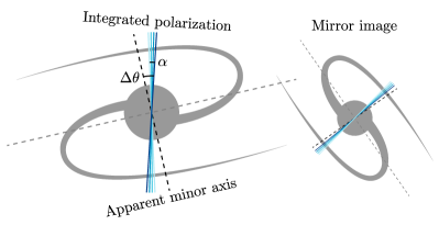
Figure 1: An illustration of the parity-violating effect cosmic birefringence has on the (mis)alignment between the linear polarization of the integrated radio emission (solid blue) and the apparent minor axis (dashed black) of a spiral galaxy. For every spiral galaxy with a mislignment angle $\Delta\theta$ (left), another galaxy whose structure is its mirror image (right) would have the opposite misalignment angle, and so $\Delta\theta$ is expected to average to zero over many galaxies. In the presence of birefringence, the integrated polarization is rotated by an angle $\alpha$ (from light to dark blue) for both the galaxy and its mirror image, and $\Delta\theta$ would be statistically biased from zero.

It has been proposed that such polarization-shape correlation can be exploited to calibrate the intrinsic shapes of galaxies, assuming that polarization is not externally modified, which reduces noise in weak lensing shear measurements [30, 31, 32]. By reversing this logic, one can calibrate the intrinsic polarization direction relative to source morphology [33, 34]. With cosmic birefringence, unrelated galaxies in a patch of the sky will have their polarization rotated by nearly the same angle, leading to a polarization-shape correlation that is biased from zero.

In this Letter, we construct a minimum-variance quadratic estimator for polarization rotation angles using a catalog of galaxies with both integrated radio polarization and shape measurements, and forecast the angular noise power spectrum for the estimator. Radio polarization measurements may come from the existing VLA Sky Survey [35] or the upcoming SKA continuum surveys [36], while the optical counterparts can come from an overlapping photometric galaxy catalog with shape measurements, such as from the DESI Legacy Surveys (DECaLS) [28] or the forthcoming LSST [29].

Galaxy Radio Polarization — When a galaxy is viewed at an inclination, the magnetic fields appear aligned with the apparent major axis. This leads to a net linear polarization of the integrated radio emission as found in [24]. The degree of polarization of the integrated emission depends on the galaxy’s disk inclination and radio luminosity, as well as the presence of a randomly oriented component of the magnetic field throughout the galaxy. Ref. [24] found in the $4.8\,\mathrm{GHz}$ emission from nearby spiral galaxies that the net degree of polarization ranges from $\sim 1\%$ to $\sim 18\%$, with a mean of $\sim 4\%$. While the alignment between the net polarization and the minor axis is not exact in any individual galaxy, the sample of [24] shows a mean misalignment angle consistent with zero and an RMS value of $\sim 26^{\circ}$. As we will see later, the effective scatter in this misalignment angle, which limits the precision of cosmic birefringence measurements, is only as small as $\sim 5^{\circ}$, once a proper quadratic estimator is constructed. This rather remarkable result is uncovered empirically from the sample of [24], which indicates a strong correlation between the scatter in misalignment angle and disk inclination.

Estimating Cosmic Birefrigence — the linear polarization of a galaxy can be described by a pair of Stokes parameters $(Q,\,U)$. A spin-2 variable $P_{\pm}$ can be defined

$$P_{\pm}\equiv Q\pm i\,U=I\,p\,e^{\pm 2\,i\,\theta_{P}},$$ (2)

where $I$ is the intensity , $p$ is the degree of polarization ($0<p<1$), and $\theta_{P}$ is the position angle of the linear polarization in the sky. The apparent elliptical shape of an inclined galaxy can be described by another spin-2 variable, the ellipticity $\epsilon_{\pm}$ [38, p. 11]

$$\epsilon_{\pm}\equiv q\pm i\,u=(a-b)/(a+b)\,e^{\pm 2\,i\,\theta_{\epsilon}},$$ (3)

where $a$ and $b$ are the semi-minor and semi-major axes, respectively, and $\theta_{\epsilon}$ is the position angle of the semi-major axis in the sky.

Since $\theta_{P}-\theta_{\epsilon}$ is invariant under rotations of the sky, we define the following (dimensionless) spin-0 quantities

$$X\pm i\,Y\equiv-P_{\pm}\,\epsilon_{\mp}/I=p\,|\epsilon|\,e^{\pm 2\,i\,\Delta\theta},$$ (4)

where $\Delta\theta\equiv\theta_{P}-\theta_{\epsilon}-\pi/2$ is the polarization-shape misalignment angle and $|\epsilon|\equiv(a-b)/(a+b)$. The quantities $X$ and $Y$ have even and odd parity, respectively.

The quantities $p$, $|\epsilon|$, and $\Delta\theta$ are intrinsic to each galaxy. Since there is no known mechanism for macroscopic parity violation in the synchrotron radiation in the interstellar medium (ISM), we assume that $\Delta\theta$ has a distribution symmetric about $\Delta\theta=0$, and that possible parity-violating effects occur externally as a result of cosmic birefringence. Cosmic birefringence can be quantified by a sightline-dependent polarization rotation field $\alpha(\bm{\mathbf{\hat{n}}})$, coherent over some angular scale on the sky. Depending on the birefringence source, $\alpha(\bm{\mathbf{\hat{n}}})$ may be uniform on the sky [39], or behave as a Gaussian random field [40, 41], or have a highly non-Gaussian spatial pattern [13]. Thus, cosmic birefringence causes the distribution of $\Delta\theta$ to be biased from zero by an amount $\alpha(\bm{\mathbf{\hat{n}}})$ for galaxies in a local sky patch in the direction $\bm{\mathbf{\hat{n}}}$. For a first analysis, we assume that $\alpha(\bm{\mathbf{\hat{n}}})$ is independent of galaxy distance, and that $(I\,p,\Delta\theta)$ are independently drawn from the same global distribution for individual galaxies.

While the Faraday effect of the Milky Way (MW)’s ISM also rotates the polarization coherently on the sky, the rotation angle scales as the wavelength squared. This can be distinguished from the wavelength-independent birefringence effect induced by an axion [11]. We therefore assume that MW Faraday rotation is subtracted as a foreground effect prior to the following analysis. This does require observation in multiple radio bands, the effectiveness of which is subject to further study. On the other hand, Faraday effect within the source galaxy causes incoherent polarization rotation across the galactic disk, which leads to the depolarization of the integrated radio emission that is stronger at lower radio frequencies [24, 42]. This is not a concern in the following analysis, as depolarization at $4.8\,\mathrm{GHz}$ is included in the empirical polarization-shape (mis)alignment data.

Parity-odd combinations of $X$ and $Y$ have a vanishing mean over the ensemble of galaxies when $\alpha(\bm{\mathbf{\hat{n}}})=0$:

$$\expectationvalue{Y}=\expectationvalue{X\,Y}=0.$$ (5)

Statistically significant deviation of $\expectationvalue{Y}$ or $\expectationvalue{XY}$ from zero would therefore be a smoking gun of parity violation.

In the presence of a nonzero $\alpha(\bm{\mathbf{\hat{n}}})$, the disk shape is unaffected while the integrated polarization is rotated:

$$P_{\pm}\to P_{\pm}\,e^{\pm 2\,i\,\alpha(\bm{\mathbf{\hat{n}}})},\quad\epsilon_{\pm}\to\epsilon_{\pm}.$$ (6)

This implies transformation rules for $X$ and $Y$

$$X \to X\,\cos 2\alpha(\bm{\mathbf{\hat{n}}})-Y\,\sin 2\alpha(\bm{\mathbf{\hat{n}}}),$$ (7)

$$Y \to Y\,\cos 2\alpha(\bm{\mathbf{\hat{n}}})+X\,\sin 2\alpha(\bm{\mathbf{\hat{n}}}).$$ (8)

Notably, the value of $\alpha(\bm{\mathbf{\hat{n}}})$ does not change observables of a galaxy along a different direction $\bm{\mathbf{\hat{n}}}^{\prime}\neq\bm{\mathbf{\hat{n}}}$.

We construct an estimator for $\alpha(\bm{\mathbf{\hat{n}}})$ using $X$ and $Y$, inspired by the minimum-variance quadratic estimators for weak lensing [43] and for polarization rotation [21, 23, 22, 44] in analyzing CMB anistropies. In App. B, this estimator is confirmed by a maximum likelihood approach [45].

For CMB anisotropies, quadratic estimators for cosmic shear and for polarization rotation are orthogonal to each other to first order in each of the effects [20]. Cosmic shear induces a white-noise $Y\approx p\,|\epsilon|\,\gamma=0.002\,(p/0.1)\,(\gamma/0.02)\,|\epsilon|$, where $\sqrt{\langle\gamma^{2}\rangle}\approx 0.02$ at $z\sim 1$ [46], which however is smaller than the intrinsic $\sigma_{Y}=0.004$ (Eq. (13)). With both weak lensing and galaxy intrinsic alignment, a correlated noise contribution to $\hat{\alpha}$ arises, but with a magnitude significantly smaller than the noise floor derived here. We will therefore disregard weak lensing in the following calculation.

To estimate the polarization rotation $\alpha(\bm{\mathbf{\hat{n}}})$ using a single galaxy in the direction $\bm{\mathbf{\hat{n}}}$, we write down an estimator $\hat{\alpha}(\bm{\mathbf{\hat{n}}})$ as the general combination of the observed quantities $\tilde{X}$ and $\tilde{Y}$ (including measurement noise) for this galaxy up to quadratic terms:

$$\hat{\alpha}\equiv u\,\tilde{X}+v\,\tilde{Y}+u^{\prime}\,\tilde{X}^{2}+v^{\prime}\,\tilde{Y}^{2}+w\,\tilde{X}\,\tilde{Y},$$ (9)

where the coefficients $u,v,u^{\prime},v^{\prime},w$ are to be determined. We omit the dependence on $\bm{\mathbf{\hat{n}}}$ for clarity of notation whenever only a single galaxy is concerned.

Following the idea underlying the minimum-variance quadratic estimator, we require that $\hat{\alpha}$ be an unbiased estimator of $\alpha$. That is, $\expectationvalue{\hat{\alpha}}=\alpha$ when averaged over an ensemble of galaxies with independent intrinsic properties. Subject to this requirement, we then minimize the variance of $\hat{\alpha}$ under the null hypothesis $\alpha=0$. To carry out the calculation analytically, we approximate $X$ as a Gaussian random variable with mean $\overline{X}$ and variance $\sigma_{X}^{2}$, and $Y$ a Gaussian random variable with zero mean and variance $\sigma_{Y}^{2}$. Since $X$ and $Y$ are only approximately Gaussian, this gives a nearly optimal quadratic estimator. The true optimal estimator could be obtained by numerically minimizing $\expectationvalue{\hat{\alpha}^{2}}$, given the empirically measured distributions for $Ip$, $|\epsilon|$, and $\Delta\theta$.

Observed quantities have measurement uncertainties. If the radio intensity measurement has an RMS uncertainty of $\sigma_{I}$, then the uncertainty on the polarization degree $p$ is $\sigma_{I}/I$, which equals the inverse unpolarized signal-to-noise ratio (SNR) of the galaxy. We find that with realistic deep optical imaging surveys that include shape measurement, the radio polarization measurement error dominates over the error in ellipticity measurement. This leads to the overall errors for $\tilde{X}$ and $\tilde{Y}$, also assumed to be Gaussian:

$$\tilde{\sigma}_{X,Y}^{2}=\sigma_{X,Y}^{2}+(1/2)\,\left(\Delta\epsilon/\mathrm{SNR}\right)^{2},$$ (10)

where $\Delta\epsilon\approx 0.3$ is the intrinsic spread in galaxy ellipticity, and $\sigma^{2}_{X,Y}$ are the intrinsic variances of $X$ and $Y$.

Since large rotation angles have been ruled out by observation, it is reasonable to assume that polarization rotation is small $\alpha\ll 1$. We find the following unbiased minimum-variance quadratic estimator (detailed derivation can be found in App. A):

$$\hat{\alpha}=\frac{\tilde{\sigma}_{Y}^{2}\,\overline{X}\,\tilde{Y}+(\sigma_{X}^{2}-\sigma_{Y}^{2})\,\tilde{X}\,\tilde{Y}}{2\left[(\sigma_{X}^{2}-\sigma_{Y}^{2})^{2}+\tilde{\sigma}_{X}^{2}\,\overline{X}^{2}\right]},$$ (11)

whose variance under the null hypothesis is

$$\expectationvalue{\hat{\alpha}^{2}}=\frac{\tilde{\sigma}_{X}^{2}\,\tilde{\sigma}_{Y}^{2}}{4\left[(\sigma_{X}^{2}-\sigma_{Y}^{2})^{2}+\tilde{\sigma}_{X}^{2}\,\overline{X}^{2}\right]}.$$ (12)

Conceptually, we have obtained the expected result that the estimator for the parity-violating $\alpha(\bm{\mathbf{\hat{n}}})$ is constructed from the parity-odd observables $Y$ and $X\,Y$ only. Since $\expectationvalue{\hat{\alpha}(\bm{\mathbf{\hat{n}}})}=0$ when $\alpha(\bm{\mathbf{\hat{n}}})=0$, a statistically significant deviation of $\expectationvalue{\hat{\alpha}(\bm{\mathbf{\hat{n}}})}$ from zero toward any direction $\bm{\mathbf{\hat{n}}}$ over a number of galaxies would be evidence for cosmic birefringence in that direction.

Sensitivity — From the observables $p$, $|\epsilon|$, and $\Delta\theta$, $X$ and $Y$ for each galaxy can be computed. We obtain values for $p$ and $\Delta\theta$ for 13 nearby spiral galaxies from Ref. [24], and compute values for $|\epsilon|$ from the angular major and minor axes given in the SIMBAD Astronomical Database [47]. We exclude M31 from that sample, as its close proximity and its particularly high degree of polarization at $18\%$ hint at possible systematics. This results in the following:

$$\overline{X}\pm\sigma_{X} =(1.3\pm 2.1)\times 10^{-2},$$

$$\overline{Y}\pm\sigma_{Y} =(0.04\pm 4.4)\times 10^{-3}.$$ (13)

Despite the small sample size used here, we find $\sqrt{\langle|\epsilon|^{2}\rangle}=0.30$, in good agreement with the typical value for cosmological samples. It is more uncertain whether the properties of the integrated radio polarization of this sample are representative of a cosmological sample. Verification would require analyses of samples of distant galaxies (e.g. [35, 48, 42]). Using values in Eq. (13) for $\overline{X}$, $\sigma_{X}$ and $\sigma_{Y}$ while fixing $\overline{Y}=0$, Eq. (12) gives the standard error in the rotation estimator for a single galaxy, $\sqrt{\expectationvalue{\hat{\alpha}^{2}}}=5^{\circ}$, for negligible measurement error.

Remarkably, $\sqrt{\expectationvalue{\hat{\alpha}^{2}}}=5^{\circ}$ is about five times smaller than the standard deviation of $\Delta\theta$ at $26^{\circ}$ as estimated from nearby spiral galaxies. We attribute this startling difference to an anti-correlation between the scatter in the misalignment angle $\Delta\theta$ and the product $p\,|\epsilon|$. According to Eq. (4), when computing the statistics of $X$ and $Y$ in Eq. (13), galaxies with large $\Delta\theta$ values are weighted less due to smaller $p\,|\epsilon|$ values.

This anti-correlation has a geometrical origin (the effect is quantitatively modelled in [24]). The intrinsic misalignment angle has a large variance for galaxies showing a low integrated polarization degree and a low ellipticity, as these galaxies mostly have a low inclination and appear rather circular. Since $p$ and $|\epsilon|$ both increase with inclination, the prefactor $p\,|\epsilon|$ effectively down-weights face-on galaxies and emphasizes edge-on galaxies on which birefringence would have a larger detectable effect. While we do not pursue it in this work, it seems possible to us that if this anti-correlation is accurately modelled as a function of the inclination, then an improved definition of $X$ and $Y$ could be derived to replace Eq. (4).

To make sure that the surprisingly small value of $\sqrt{\langle\hat{\alpha}^{2}\rangle}=5^{\circ}$ is not a fluke of low-number statistics from only 13 galaxies, we perform bootstrapping on the data extracted from Refs. [24, 47]. In each run, 4,000 pairs of $(p|\epsilon|,\Delta\theta)$ are generated by independent draws from the 13 galaxies with replacement. The value of $\expectationvalue{\hat{\alpha}^{2}}$ is then computed from the $4,000$ artificial pairs using Eq. (12). We repeat this procedure 2,000 times, and obtain $\sqrt{\expectationvalue{\hat{\alpha}^{2}}}=(44\pm 5)^{\circ}$ (see Fig. 2), strongly suggesting that the anti-correlation between $\Delta\theta$ and $p\,|\epsilon|$ is real.

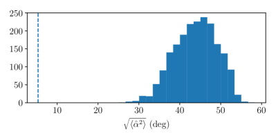
Figure 2: Histogram of the standard error of $\hat{\alpha}$ when the anti-correlation between $p|\epsilon|$ and $\Delta\theta$ is erased by bootstrapping using a sample of 13 galaxies, repeated 2,000 times. The dashed line marks the standard error of $\hat{\alpha}$ measured from the 13 galaxies without boostrapping. Its significantly lower value compared to the bootstrapped distribution indicates that there is a genuine anti-correlation between $\Delta\theta$ and $p\,|\epsilon|$.

Galaxy Survey — Under the flat-sky approximation, the estimator is given by a finite sum over $N$ discrete galaxies

$$\hat{\alpha}(\mathbf{L})=(\Omega/N)\,\sum_{i=1}^{N}\,e^{-i\mathbf{L}\cdot\bm{\mathbf{\hat{n}}}_{i}}\,\hat{\alpha}(\bm{\mathbf{\hat{n}}}_{i}),$$ (14)

where $\Omega$ is survey area in steradians. The variance of the estimator is then

$$\expectationvalue{\hat{\alpha}(\mathbf{L})\,\hat{\alpha}(\mathbf{L}^{\prime})^{*}}=(\Omega/N)^{2}\,\expectationvalue{\hat{\alpha}^{2}}\sum_{i=1}^{N}e^{-i\,(\mathbf{L}-\mathbf{L}^{\prime})\cdot\bm{\mathbf{\hat{n}}}_{i}}.$$ (15)

When galaxies are dense on the sky, the sum approximates a Dirac delta function:

$$\expectationvalue{\hat{\alpha}(\mathbf{L})\,\hat{\alpha}(\mathbf{L}^{\prime})^{*}}=(\Omega/N)\,\expectationvalue{\hat{\alpha}^{2}}(2\pi)^{2}\,\delta^{(2)}(\mathbf{L}-\mathbf{L}^{\prime}).$$ (16)

In the absence of birefringence, the estimation for the rotation power spectrum is therefore limited by a white-noise floor

$$C_{\hat{\alpha}\hat{\alpha}}(\mathbf{L})=(\Omega/N)\,\expectationvalue{\hat{\alpha}^{2}},$$ (17)

analogous to the shot noise in cosmic shear estimation from a discrete sample of galaxies.

We adapt the procedure used in Ref. [49] to count the number of available spiral galaxies. We first compute the redshift-dependent radio luminosity function of spiral galaxies. The radio luminosity function at $4.8\,\mathrm{GHz}$ at redshift $z$ can be expressed in terms of the radio luminosity function at $1.4\,\mathrm{GHz}$ at $z=0$, taking into account luminosity evolution [50] and the spectral index ($S_{\nu}\propto\nu^{\alpha}$ where $\alpha=-0.7$ [51, 52]). We choose $4.8\,\mathrm{GHz}$ because Ref. [24] established the empirical correlation at this frequency and because Faraday rotation in both the source and the MW is greatly reduced at higher frequencies. Next, the local radio luminosity function can be obtained from the far-infrared (FIR) luminosity function [53, 54] by exploiting an approximately linear relation between the radio and FIR luminosities of star-forming galaxies [55, 56].

The number of spiral galaxies with an observed spectral flux density $S_{\nu}$ above a threshold $S_{\nu}^{\mathrm{min}}$ is given by

$$N[S_{\nu}>S_{\nu}^{\mathrm{min}}]=$$ (18)

$$\quad\Omega\int{\rm d}z\int_{\log\lambda(z)^{-1}L_{4.8}^{\mathrm{min}}(z)}^{\log L_{4.8}^{\mathrm{max}}}\,{\rm d}\log L_{4.8}\,\frac{c\,s(z)^{2}}{H(z)}\,\phi(\log L_{4.8}),$$

where $s(z)=\int_{0}^{z}c/H(z^{\prime})\,{\rm d}z^{\prime}$ is the comoving distance to redshift $z$; $H(z)$ is the expansion rate for $H_{0}=70\,\mathrm{km\,s^{-1}\,Mpc^{-1}},\Omega_{\Lambda}=0.7,\Omega_{m}=0.3$; $\Omega$ is the surveyed sky area in steradians; $\phi$ is the $4.8\,\mathrm{GHz}$ radio luminosity function (per unit comoving volume) of spiral galaxies at $z=0$ (details can be found in App. D); $L_{4.8}^{\mathrm{max}}=10^{25}\,\mathrm{W\,Hz^{-1}}$ is a generous upper bound on the radio luminosity of a spiral galaxy; $L_{4.8}^{\mathrm{min}}$ is the luminosity of a galaxy at redshift $z$ with an observed spectral flux density of $S_{\nu}^{\mathrm{min}}$:

$$L_{4.8}^{\mathrm{min}}(z)=4\pi\,s(z)^{2}\,(1+z)^{1-\alpha}\,S_{\nu}^{\mathrm{min}};$$ (19)

and $\lambda(z)$ describes the luminosity evolution with $z$ for spiral galaxies [50]. The upper limit in the $z$ integral should not exceed $z=1.5$; above that, nearly all massive halos host spheroidal galaxies [57]. The lower limit in the $z$ integral ideally should exceed the redshift of detectable sources of birefringence. There is then a trade-off between the galaxy number and the accumulation of birefringence along the line of sight. A more sophisticated treatment would consider birefringence sources interspersed amongst the galaxies throughout all redshift $0<z<1.5$. We leave such model-dependent calculations to a future study.

The highest sensitivity achievable with available data in the near future will likely come from correlating polarized SKA radio galaxies with LSST shape data (or using radio shapes from resolved SKA images). Similar to Ref. [58], we consider Wide, Deep, and Ultradeep reference surveys, which have $\sigma_{I}=1\,\mathrm{\mu Jy}$, $0.2\,\mathrm{\mu Jy}$, and $0.05\,\mathrm{\mu Jy}$, and cover $1000\,\mathrm{deg}^{2}$, $20\,\mathrm{deg}^{2}$, and $1\,\mathrm{deg}^{2}$ on the sky, respectively, but for SKA-MID Band 5a ($4.6$–$8.5\,$GHz [59]). Including galaxies whose integrated radio intensities have ${\rm SNR}>5$ at $4.8\,\mathrm{GHz}$, we estimate the number of measurable spiral galaxies at $0.2<z<1.5$ to be $N=1.6\times 10^{6}$, $2.1\times 10^{5}$ and $2.8\times 10^{4}$ for each survey, respectively. For $0.8<z<1.5$, the numbers are $N=2.8\times 10^{5}$, $9.5\times 10^{4}$ and $1.7\times 10^{4}$, respectively. App. D details the calculation behind these numbers.

While most detectable galaxies will have polarization measurement errors making an important contribution to the variance of the estimator $\hat{\alpha}$, they collectively provide a non-negligible amount of information to reduce the variance in the estimation of $\alpha$. Consider $N$ detectable spiral galaxies in a small sky patch ${\rm d}\Omega$, each with a rotation estimator $\hat{\alpha}_{i}$. From a general linear combination $\hat{\alpha}_{\mathrm{best}}\equiv\sum^{N}_{i=1}w_{i}\,\hat{\alpha}_{i}$, we can obtain the weights that lead to an unbiased minimum-variance estimator, namely $w_{i}=\expectationvalue{\hat{\alpha}_{i}^{2}}^{-1}/\sum_{j}\expectationvalue{\hat{\alpha}_{j}^{2}}^{-1}$. For different galaxies, $\expectationvalue{\hat{\alpha}_{i}^{2}}$ only depends on the unpolarized radio SNR, which in turn only depends on $z$ and $L_{4.8}$. Let us denote it as $\expectationvalue{\hat{\alpha}^{2}}(x)$, where $x=(z,\,\log L_{4.8})$.

With Eq. (18) rewritten as $N={\rm d}\Omega\,\int\Phi(x)\,{\rm d}x$, the weights take the form

$$w(x)={\rm d}\Omega^{-1}\,\expectationvalue{\hat{\alpha}^{2}}(x)^{-1}\,\left[\int\expectationvalue{\hat{\alpha}^{2}}(x^{\prime})^{-1}\Phi(x^{\prime})\,{\rm d}x^{\prime}\right]^{-1},$$ (20)

where $\Phi(x)$ quantifies the galaxy distribution with redshift and luminosity as defined in Eq. (40). This leads to

$$\expectationvalue{\hat{\alpha}_{\mathrm{best}}^{2}}={\rm d}\Omega^{-1}\left[\int\expectationvalue{\hat{\alpha}^{2}}(x)^{-1}\Phi(x)\,{\rm d}x\right]^{-1}.$$ (21)

Accounting for the SNR distribution is therefore equivalent to having $N$ identically measured galaxies, each with an effective estimator variance of

$$\expectationvalue{\hat{\alpha}^{2}}_{\mathrm{eff}}=N\expectationvalue{\hat{\alpha}_{\mathrm{best}}^{2}}=\frac{\int\Phi(x)\,{\rm d}x}{\int\expectationvalue{\hat{\alpha}(x^{\prime})^{2}}^{-1}\Phi(x^{\prime})\,{\rm d}x^{\prime}}.$$ (22)

We replace $\expectationvalue{\hat{\alpha}^{2}}$ in Eq. (17) with $\expectationvalue{\hat{\alpha}^{2}}_{\rm eff}$ to estimate the effective noise power spectrum

$$C_{\hat{\alpha}\hat{\alpha}}(\mathbf{L})=\left[\int\expectationvalue{\hat{\alpha}(x)^{2}}^{-1}\Phi(x)\,{\rm d}x\right]^{-1}.$$ (23)

While the $x$-integration formally depends on the choice of the threshold intensity $S_{\nu}^{\mathrm{min}}$ as in Eq. (18), the integral approaches a minimal value as $S_{\nu}^{\mathrm{min}}$ decreases, until it is practically saturated for $S_{\nu}^{\mathrm{min}}/\sigma_{I}\lesssim 5$.

In Fig. 3, the noise angular power spectrum of the rotation estimator is plotted, along with the corresponding sensitivity curves for current and projected CMB surveys [20]. SKA will enable a noise power spectrum lower than that of CMB-S4 for $L\gtrsim 5$, but probe a more limited $z$ range for the birefringence sources. The noise spectra are compared to the maximal signal allowed by Planck [20] due to a network of ultralight axion strings [13] approximated by the loop crossing model [60].

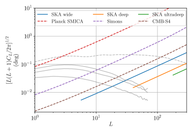
Figure 3: Polarization rotation noise power spectra for SKA radio galaxy surveys combined with an overlapping optical imaging galaxy survey, compared to those for three CMB surveys. The low-$L$ cutoffs of SKA curves are set by the proposed survey areas. We show signal power spectra from ultralight axion strings (see main text) up to $z=z_{\mathrm{cmb}}$ (gray dashed) and up to $z=1.5,\,1,\,0.5$ (gray solid; from top to bottom).

Discussion — Using Eq. (11), noisy rotation estimations can be done at discrete galaxy locations $\{\hat{\alpha}_{i}\}_{i}$, which is suited for real-space approaches that exploit the non-Gaussian statistics of $\alpha(\bm{\mathbf{\hat{n}}})$. This is applicable to birefringence from an axion string network [61, 62].

Measuring polarization rotation in the CMB has the advantage of being sensitive to all birefringence sources up to $z\approx 1100$. Spiral galaxies do not effectively probe birefringence sources at $z\gtrsim 1.5$. Nonetheless, galaxies present an opportunity for extracting tomographic information, i.e. the $z$-dependence of the birefringence sources. One could compare rotation estimated from the CMB with that from radio galaxies, or compare estimates from galaxies in different $z$ bins. For example, if axion strings exist for much of the cosmic history, this would enable the measurement of their size and number evolution with $z$ [60]. Furthermore, an axion field that is homogeneous but dynamic for $z\lesssim 1100$ is indistinguishable from a constant uniform axion field via a CMB measurement, but could show up as $z$-dependent in galaxy-based birefringence tomography. This also means that any detection of cosmic birefringence through the CMB [14] can then be validated through galaxy surveys. Foreground systematics that are unaccounted for, e.g. from the MW, would show up coherently for galaxies in every redshift bin and could thus be identified and subtracted.

Conclusion — We have proposed a new statistical technique to estimate anisotropic cosmic birefringence from correlation between radio polarization and shape in spiral galaxies. This offers an independent technique that complements CMB probes. This will be enabled by a synergy between upcoming large radio galaxy surveys such as SKA and optical imaging surveys such as LSST. The noise floor of the polarization rotation angular power spectrum of the galaxy-based method using SKA will be better than that of CMB-S4. We plan to test the empirical correlations of [24] on cosmological galaxy samples using data from existing smaller radio surveys [35, 48, 42].

Appendix A Quadratic estimator

Polarization and shape measurements have errors. For example, the polarized flux has a squared error

$$\sigma_{P}^{2}=\frac{\sigma_{I}^{2}}{2},$$ (24)

where $\sigma_{I}$ is the RMS flux of the detector in units of Jansky. We assume that the effect of measurement errors on the variance of the quadratic estimator $\hat{\alpha}$ is dominated by the measurement error for polarization, and the shape error is much smaller. In this case,

$$\tilde{\sigma}_{X,Y}^{2}=\sigma_{X,Y}^{2}+\frac{\sigma_{I}^{2}\,\sigma_{\epsilon}^{2}}{2\,I^{2}}=\sigma_{X,Y}^{2}+\frac{\sigma_{\epsilon}^{2}}{2\,\mathrm{SNR}^{2}},$$ (25)

where the total flux SNR enters the expression.

We now calculate the propagation of this error into the variance of the quadratic estimator. Let $\hat{\alpha}$ for each galaxy be constructed from the observed quantities (with tilde) including measurement errors, up to quadratic combinations:

$$\hat{\alpha}\equiv u\,\tilde{X}+v\,\tilde{Y}+u^{\prime}\,\tilde{X}^{2}+v^{\prime}\,\tilde{Y}^{2}+w\,\tilde{X}\,\tilde{Y},$$ (26)

where the coefficients are to be determined. Under a polarization rotation $\alpha$ at the galaxy’s location, the observed quantities are transformed:

$$\tilde{X}\to\tilde{X}-2\alpha\,Y,\quad\tilde{Y}\to\tilde{Y}+2\alpha\,X.$$ (27)

Note that the transformation is proportional to quantities without measurement noises, since cosmic birefringence is applied before detection. By requiring that the estimator $\hat{\alpha}$ be unbiased, namely $\expectationvalue{\hat{\alpha}}=\alpha$, we have

$$0 =u\expectationvalue{X}+u^{\prime}\expectationvalue{X^{2}}+v^{\prime}\expectationvalue{Y^{2}}$$ (28)

$$\frac{1}{2} =v\expectationvalue{X}+w\expectationvalue{X^{2}}-w\expectationvalue{Y^{2}}.$$ (29)

Using these, $u$ can be expressed in terms of $u^{\prime}$ and $v^{\prime}$, and $v$ can be expressed in terms of $w$. It remains to minimize the variance of the estimator, $\expectationvalue{\hat{\alpha}^{2}}$, under the null hypothesis, with respect to $u^{\prime}$, $v^{\prime}$, and $w$. After some algebra, we obtain the claimed result in Eq. (11):

$$u=u^{\prime}=v^{\prime}=0,\quad v=\frac{\tilde{\sigma}_{Y}^{2}\,\overline{X}}{2\left[(\sigma_{X}^{2}-\sigma_{Y}^{2})^{2}+\tilde{\sigma}_{X}^{2}\,\overline{X}^{2}\right]},\quad w=\frac{\sigma_{X}^{2}-\sigma_{Y}^{2}}{2\left[(\sigma_{X}^{2}-\sigma_{Y}^{2})^{2}+\tilde{\sigma}_{X}^{2}\,\overline{X}^{2}\right]}.$$ (30)

Appendix B Maximum likelihood approach

Inspired by the idea originally put forth in Ref. [45] and closely following the formalism presented in Ref. [20], we pursue an maximum-likelihood approach to estimating the polarization rotation field $\alpha(\bm{\mathbf{\hat{n}}})$. For detailed justifications of some assumptions we are about to make, we refer to Sections 3 and 4.1 of Ref. [20].

Let $\mathbf{X}_{i}\equiv\begin{pmatrix}\tilde{X}_{i}&\tilde{Y}_{i}\end{pmatrix}^{T}$ denote the observed quantities including measurement error for the $i$-th galaxy, located in the direction $\bm{\mathbf{\hat{n}}}_{i}$, among a total of $N$ galaxies. We start by assuming the following log-likelihood function:

$$\ln\mathcal{L}[\alpha;\{\mathbf{X}_{i},\mathbf{N}_{i}\}]=-\frac{1}{2}\sum_{i=1}^{N}\left\{\left[M(\alpha(\bm{\mathbf{\hat{n}}}_{i}))^{-1}(\mathbf{X}_{i}-\mathbf{N}_{i})-\overline{\mathbf{X}}_{i}\right]^{T}\,C_{\mathbf{X}_{i}}^{-1}\,\left[M(\alpha(\bm{\mathbf{\hat{n}}}_{i}))^{-1}(\mathbf{X}_{i}-\mathbf{N}_{i})-\overline{\mathbf{X}}_{i}\right]+\mathbf{N}_{i}^{T}C_{\mathbf{N}_{i}}^{-1}\mathbf{N}_{i}\right\},$$ (31)

where $\mathbf{N}_{i}$ is the measurement error of $\mathbf{X}_{i}$; $\overline{\mathbf{X}}_{i}$ is the mean of $\mathbf{X}$ over an ensemble of galaxies; $C_{\mathbf{X}_{i}}$ is the covariance matrix of the intrinsic, unrotated quantities $\mathbf{X}_{i}$ (which in general may depend on the type or other properties of the $i$-th galaxy); $C_{\mathbf{N}_{i}}$ is the covariance matrix of the measurement noise given by the second term in Eq. (10); and $M(\alpha(\bm{\mathbf{\hat{n}}}_{i}))$ is the effect of polarization rotation on the intrinsic quantities. Eq. (31) assumes that each $\mathbf{X}_{i}$ is a random Gaussian variable, the same approximation we used in the main text, meaning $C_{\mathbf{X}_{i}}=\operatorname{diag}(\tilde{\sigma}_{X_{i}}^{2},\tilde{\sigma}_{Y_{i}}^{2})$. Our goal is then to obtain an estimator $\hat{\alpha}_{\mathrm{ML}}(\bm{\mathbf{\hat{n}}})$ which maximizes $\ln\mathcal{L}$ given a set of observations $\{\mathbf{X}_{i}\}$.

Since the sum in Eq. (31) has completely independent terms, it suffices to individually maximize each term:

$$\ln\mathcal{L}_{i}[\alpha(\bm{\mathbf{\hat{n}}}_{i});\mathbf{X}_{i},\mathbf{N}_{i}]=-\frac{1}{2}\left[M(\alpha(\bm{\mathbf{\hat{n}}}_{i}))^{-1}(\mathbf{X}_{i}-\mathbf{N}_{i})-\overline{\mathbf{X}}_{i}\right]^{T}\,C_{\mathbf{X}_{i}}^{-1}\,\left[M(\alpha(\bm{\mathbf{\hat{n}}}_{i}))^{-1}(\mathbf{X}_{i}-\mathbf{N}_{i})-\overline{\mathbf{X}}_{i}\right]-\frac{1}{2}\mathbf{N}_{i}^{T}C_{\mathbf{N}_{i}}^{-1}\mathbf{N}_{i}.$$ (32)

From now on, we will omit the galaxy index $i$ and suppress the $\bm{\mathbf{\hat{n}}}_{i}$ dependence for clarity. For any fixed $\mathbf{X}$, the likelihood is maximized when the noise is

$$\mathbf{N}_{\mathrm{max}}=(\mathbf{M}^{-T}C_{\mathbf{X}}^{-1}\mathbf{M}^{-1}+C_{\mathbf{N}}^{-1})^{-1}\mathbf{M}^{-T}C_{\mathbf{X}}^{-1}(\mathbf{M}^{-1}\mathbf{X}-\overline{\mathbf{X}}).$$ (33)

The value of the likelihood at this noise realisation is

$$\ln\mathcal{L}[\alpha;\mathbf{X},\mathbf{N}=\mathbf{N}_{\mathrm{max}}]=-\frac{1}{2}(\mathbf{X}-\mathbf{M}^{-1}\overline{\mathbf{X}})^{-1}(C_{\mathbf{N}}+\mathbf{M}^{T}C_{\mathbf{X}}\mathbf{M})^{-1}(\mathbf{X}-\mathbf{M}^{-1}\overline{\mathbf{X}}).$$ (34)

It would have been more justifiable to marginalize over the noise $\mathbf{N}$, which would produce an additional logarithmic term that is numerically negligible.

The matrix $M(\alpha)$ depends on the angle $\alpha$ non-linearly. Using Eqs. (7)–(8), we expand it up to $O(\alpha^{2})$:

$$M(\alpha)=e^{2\,\alpha\,T}=1+2\,\alpha\,T+2\,\alpha^{2}\,T^{2},\quad T=\begin{pmatrix}0&1\\ -1&0\end{pmatrix}.$$ (35)

We insert this expansion into Eq. (34) and take the derivative with respect to $\alpha$, keeping terms up to linear order:

$$\frac{\partial\mathcal{L}}{\partial\alpha}=\frac{2}{\tilde{\sigma}_{X}^{2}\,\tilde{\sigma}_{Y}^{2}}\left[\tilde{\sigma}_{Y}^{2}\,\overline{X}\,\tilde{Y}+(\sigma_{X}^{2}-\sigma_{Y}^{2})\,\tilde{X}\,\tilde{Y}\right]-\frac{4\,\alpha}{\tilde{\sigma}_{X}^{4}\,\tilde{\sigma}_{Y}^{4}}\left[(\cdots)+(\cdots)\tilde{X}+(\cdots)\tilde{X}^{2}+(\cdots)\tilde{Y}^{2}\right],$$ (36)

where $(\cdots)$ are combinations of statistical quantities whose exact forms are not enlightening. This results in the maximum-likelihood estimator

$$\hat{\alpha}_{\mathrm{ML}}=\frac{\tilde{\sigma}_{X}^{2}\,\tilde{\sigma}_{Y}^{2}\left[\tilde{\sigma}_{Y}^{2}\,\overline{X}\,\tilde{Y}+(\sigma_{X}^{2}-\sigma_{Y}^{2})\,\tilde{X}\,\tilde{Y}\right]}{2\left[(\cdots)+(\cdots)\tilde{X}+(\cdots)\tilde{X}^{2}+(\cdots)\tilde{Y}^{2}\right]}.$$ (37)

We then introduce the approximation by replacing the denominator of the estimator with its ensemble average (expectation value):

$$\hat{\alpha}_{\mathrm{ML}}=\frac{\tilde{\sigma}_{X}^{2}\,\tilde{\sigma}_{Y}^{2}\left[\tilde{\sigma}_{Y}^{2}\,\overline{X}\tilde{Y}+(\sigma_{X}^{2}-\sigma_{Y}^{2})\,\tilde{X}\,\tilde{Y}\right]}{2\left[(\cdots)+(\cdots)\overline{X}+(\cdots)(\tilde{\sigma}_{X}^{2}+\overline{X}^{2})+(\cdots)\tilde{\sigma}_{Y}^{2}\right]}.$$ (38)

After some simplification, the quadratic estimator in Eq. (11) is recovered:

$$\hat{\alpha}_{\mathrm{ML}}=\frac{\tilde{\sigma}_{Y}^{2}\,\overline{X}\,\tilde{Y}+(\sigma_{X}^{2}-\sigma_{Y}^{2})\,\tilde{X}\,\tilde{Y}}{2\left[(\sigma_{X}^{2}-\sigma_{Y}^{2})^{2}+\tilde{\sigma}_{X}^{2}\,\overline{X}^{2}\right]},$$ (39)

which agrees with the quadratic estimator Eq. (11). When $\alpha=0$, the variance $\expectationvalue{\hat{\alpha}_{\mathrm{ML}}^{2}}$ is therefore also given by Eq. (12).

Appendix C Effective estimator variance

Eq. (12) and Eq. (10) tell us the dependence of the estimator error $\sqrt{\expectationvalue{\hat{\alpha}^{2}}}$ on the RMS flux $\sigma_{I}$ of a given radio survey. For a cosmological sample of galaxies, we can use the redshift-dependent radio luminosity function of galaxies to obtain a distribution of values for $\expectationvalue{\hat{\alpha}^{2}}$ when measurement errors are accounted for.

We wish to include as many galaxies as possible in our estimation of $\alpha$, even if many may have low SNR for the polarized flux. We now calculate the lowest estimator variance achievable by including all galaxies observable by an experiment with a given $\sigma_{I}$.

Suppose we are estimating the birefringence $\alpha$ within a small solid angle ${\rm d}\Omega$ around a direction $\bm{\mathbf{\hat{n}}}$. The galaxies located within this patch of sky follow the redshift-dependent radio luminosity function. That is, in a redshift bin from $z$ to $z+{\rm d}z$ and a luminosity bin from $\log L$ to $\log L+{\rm d}\log L$, the number of galaxies in a solid angle ${\rm d}\Omega$ is

$${\rm d}N=\Phi(z,\log L)\,{\rm d}z\,{\rm d}\log L\,{\rm d}\Omega.$$ (40)

Each of these galaxies corresponds to an independent estimator $\hat{\alpha}_{i}$ whose variance $\expectationvalue{\hat{\alpha}(p)^{2}}$ only depends on $p=(z,\log L)$ of the galaxy. We define a new estimator as a linear combination of them:

$$\hat{\alpha}_{\mathrm{best}}\equiv\sum_{i}w_{i}\,\hat{\alpha}_{i}.$$ (41)

The weights are required to sum to unity:

$$1=\sum_{i}\,w_{i}.$$ (42)

We assume that the weight $w_{i}=w(p)$ only depends on $p$. In the continuum limit, we have

$$1={\rm d}\Omega\,\int w(p)\,\Phi(p)\,{\rm d}p.$$ (43)

Under this constraint, we choose weights that minimise the variance of $\hat{\alpha}_{\mathrm{best}}$:

$$\expectationvalue{\hat{\alpha}_{\mathrm{best}}^{2}}=\sum_{ij}w_{i}w_{j}\expectationvalue{\hat{\alpha}_{i}\hat{\alpha}_{j}}=\sum_{i}w_{i}^{2}\expectationvalue{\hat{\alpha}_{i}^{2}}.$$ (44)

In the continuum limit, this can be written as

$$\expectationvalue{\hat{\alpha}_{\mathrm{best}}^{2}}={\rm d}\Omega\,\int w(p)^{2}\expectationvalue{\hat{\alpha}(p)^{2}}\Phi(p)\,{\rm d}p.$$ (45)

A standard application of the Lagrange multiplier method leads to

$$w(p)={\rm d}\Omega^{-1}\,\left[\int\expectationvalue{\hat{\alpha}(p^{\prime})^{2}}^{-1}\,\Phi(p^{\prime})\,{\rm d}p^{\prime}\right]^{-1}\,\expectationvalue{\hat{\alpha}(p)^{2}}^{-1}.$$ (46)

The minimum variance is

$$\expectationvalue{\hat{\alpha}_{\mathrm{best}}^{2}}={\rm d}\Omega^{-1}\,\left[\int\expectationvalue{\hat{\alpha}(p^{\prime})^{2}}^{-1}\,\Phi(p^{\prime})\,{\rm d}p^{\prime}\right]^{-1}.$$ (47)

This is the best estimator variance achieved from a total of $N$ galaxies following the luminosity function, where

$$N={\rm d}\Omega\,\int\Phi(p)\,{\rm d}p.$$ (48)

If there were instead $N$ galaxies with the same estimator variance $\expectationvalue{\hat{\alpha}^{2}}_{\mathrm{eff}}$, the variance of the arithmetic mean of their corresponding estimators would be $\expectationvalue{\hat{\alpha}^{2}}_{\mathrm{eff}}/N$. What would $\expectationvalue{\hat{\alpha}^{2}}_{\mathrm{eff}}$ have to be so that the arithmetic mean would produce the same variance as $\hat{\alpha}_{\mathrm{best}}$? The answer is

$$\expectationvalue{\hat{\alpha}^{2}}_{\mathrm{eff}}=N\,\expectationvalue{\hat{\alpha}_{\mathrm{best}}^{2}}=\frac{\int\Phi(p)\,{\rm d}p}{\int\expectationvalue{\hat{\alpha}(p)^{2}}^{-1}\Phi(p)\,{\rm d}p},$$ (49)

which is correctly independent of the solid angle ${\rm d}\Omega$.

We can use this $\expectationvalue{\hat{\alpha}^{2}}_{\mathrm{eff}}$ to estimate the noise floor of the power spectrum:

$$C_{\hat{\alpha}\hat{\alpha}}=\frac{\Omega}{N_{\mathrm{tot}}}\,\expectationvalue{\hat{\alpha}^{2}}_{\mathrm{eff}}=\frac{\Omega}{N_{\mathrm{tot}}}\frac{\int\Phi(p)\,{\rm d}p}{\int\expectationvalue{\hat{\alpha}(p)^{2}}^{-1}\,\Phi(p)\,{\rm d}p}=\left[\int\expectationvalue{\hat{\alpha}(p)^{2}}^{-1}\,\Phi(p)\,{\rm d}p\right]^{-1},$$ (50)

which is independent of the sky area surveyed.

Appendix D Radio luminosity function

In this Appendix, we outline our procedure for estimating the source count of spiral galaxies for radio continuum surveys, thus providing the calculation details underlying Eq. (18).

The number of galaxies observable within a solid angle ${\rm d}\Omega$ of the sky, in a redshift interval between $z$ and $z+{\rm d}z$ and in a logarithmic interval of intrinsic spectral luminosity between $\log L$ and $\log L+{\rm d}\log L$, can be written as

$${\rm d}N=\frac{c\,s^{2}(z)}{H(z)}\,\phi(z,\log L)\,{\rm d}\Omega\,{\rm d}z\,{\rm d}\log L,$$ (51)

where the luminosity function $\phi(z,\log L)$ gives the number density (per unit comoving volume) of galaxies per decade of luminosity at redshift $z$, and $c\,s(z)^{2}/H(z)\,{\rm d}\Omega\,{\rm d}z$ is the comoving volume corresponding to the solid angle ${\rm d}\Omega$ and the redshift slice from $z$ to $z+{\rm d}z$. We need to know the functional form of $\phi$ for radio-emitting spiral galaxies.

The radio galaxy luminosity function $\phi$ at $z>0$ can be related to that at $z=0$:

$$\phi(z,\log L)=\phi(0,\log[\lambda(z)L]),$$ (52)

where the factor $\lambda(z)$ accounts for the redshift evolution of spiral galaxies. For this, we adopt the simple formula from [63] that fits observed counts (also see [50]):

$$\lambda(z)=\begin{cases}(1+z)^{-1.5},&0\leq z<1\\ 2^{-1.5},&1\leq z<1.5\end{cases}.$$ (53)

The number density of spiral galaxies appear to drop quickly above $z=1.5$ [57], so we set $\phi(z,\log L)=0$ for $z\geq 1.5$.

Suppose the radio luminosity function $\phi_{\nu}(z,\log L)$ at some frequency $\nu$ is known. The function at a different frequency $\nu^{\prime}$ can be derived as:

$$\phi_{\nu^{\prime}}(z,\log L)=\phi_{\nu}(z,\log[(\nu^{\prime}/\nu)^{-\alpha}L]),$$ (54)

by exploiting the power-law frequency dependence of the spectral flux density with respect to frequency: $S_{\nu}\propto\nu^{\alpha}$, where the spectral index has an appropriate value $\alpha=-0.7$ [51, 52]. While [24] reported the empirical polarization-shape correlation at $4.8\,$GHz, we would like to relate sources at $4.8\,$GHz to sources at $\nu=1.4\,$GHz in order to make contact with observed counts.

For local star-forming galaxies, it is known that the radio and far infrared (FIR) luminosities are nearly linearly related [64, 65, 66, 67]. Consider a general mean relation between the FIR luminosity and the radio luminosity at $z=0$:

$$L_{1.4}=f(L_{\mathrm{FIR}}).$$ (55)

The corresponding luminosity functions at $z=0$ are related by

$$\phi_{1.4}(0,\log L_{1.4})=\frac{L_{1.4}}{f^{-1}(L_{1.4})\,f^{\prime}(f^{-1}(L_{1.4}))}\,\phi_{\mathrm{FIR}}(f^{-1}(\log L_{1.4})),$$ (56)

where $f^{-1}$ is the inverse function to $f$. This reduces to a simple shift in the logarithmic luminosity when $f$ is linear.

The FIR luminosity function is given by a phenomenological Schechter model [53]:

$$\phi_{\mathrm{FIR}}(\log L_{\mathrm{FIR}})=\phi_{*}\left(\frac{L_{\mathrm{FIR}}}{L_{*}}\right)^{1-a}\exp{-\frac{1}{2\,\sigma^{2}}\left[\log(1+\frac{L_{\mathrm{FIR}}}{L_{*}})\right]^{2}}.$$ (57)

The parameter values are taken from Eq. (6) in [53], which correspond to the “cool” galaxies, which are interpreted as star-forming spiral galaxies. Corrections from [54] are applied, assuming $h=0.7$:

$$\phi_{*}=0.635\,\mathrm{Mpc^{-3}},\quad a=1.25,\quad L_{*}=1.95\times 10^{9}\,L_{\odot},\quad\sigma=0.5.$$ (58)

Following Eq. (16) in [56], we find that the following fitting function for Eq. (55) in combination with the FIR luminosity function above reproduces the appropriate curve in Fig. 8 of [56]:

$$L_{1.4}=A\left[\left(\frac{L_{\mathrm{FIR}}}{L_{b}}\right)^{-3.1}+\left(\frac{L_{\mathrm{FIR}}}{L_{b}}\right)^{-1}\right]^{-1},$$ (59)

where the fitting parameters are given as

$$A=7.66\times 10^{20}\,\mathrm{W\,Hz^{-1}},\quad L_{b}=3.34\times 10^{35}\,\mathrm{W}.$$ (60)

Having found the redshift-dependent radio luminosity function $\phi_{\nu}(z,\log L)$ for any radio frequency $\nu$, we can now compute the total source count within a sky patch by integrating Eq. (51):

$$N=\Omega\int{\rm d}z\int_{L_{\mathrm{min}}}^{L_{\mathrm{max}}}{\rm d}\log L\,\frac{c\,s(z)^{2}}{H(z)}\,\phi_{\nu(z)}(z,\log L),$$ (61)

where $\nu(z)=\nu_{0}\,(1+z)$ is the intrinsic frequency at the location of a galaxy at redshift $z$ corresponding to an observed frequency $\nu_{0}$. If the radio continuum survey has an RMS flux of $S_{\nu}^{\mathrm{min}}$, then the luminosity cutoff is given by

$$L_{\mathrm{min}}=4\pi\,s(z)^{2}\,(1+z)\,S_{\nu}^{\mathrm{min}}.$$ (62)

Writing $\phi(\log L)\equiv\phi_{\nu_{0}}(0,\log L)$ and performing a change of variables on $\log L$ from $1.4\,$GHz to $4.8\,$GHz, we derive Eq. (18) in the main text.