Primordial Magnetic Fields in Light of Dark Ages Global 21-cm Signal

Abstract

We study the constraints on the primordial magnetic fields in light of dark ages global 21-cm signal. An early absorption signal in the redshift of 200 $\lesssim z\lesssim$ 30 is predicted in the $\Lambda$CDM model of cosmology. During the Dark Ages, there were no stars, therefore, measuring the global 21-cm signal can provide pristine cosmological information. However, measuring the Dark Ages global 21-cm signal from ground-based telescopes is challenging. To overcome this difficulty, recently lunar and space-based experiments have been proposed, such as FARSIDE, DAPPER, FarView, etc. Primordial magnetic fields can heat the intergalactic medium gas via magnetohydrodynamic effects. We study the effects of magnetic fields on the Dark Ages global 21-cm signal and constrain the present-day strength of primordial magnetic fields and the spectral index. We find that measuring the Dark Ages signal can provide stronger bounds compared to the existing constraints from Planck 2016. Additionally, we also explore the dark-ages consistency ratio which can identify the magnetic heating of IGM by measuring the 21-cm signal at only three different redshifts in future experiments.

1 Introduction

After the recombination epoch ending around a redshift of $z\approx 1100$, the primordial plasma predominantly contained neutral hydrogen gas. In addition to neutral hydrogen, residual free electrons and protons, and the free streaming photons filled the early Universe. The photons get decoupled from the plasma and are observed today as the cosmic microwave background radiation (CMB). Due to the hyperfine transition between $F=1$ and $F=0$ states in neutral hydrogen, it can emit a photon of a wavelength of 21 cm. The relative population density of neutral hydrogen atoms in $F=1$ and $F=0$ states at a temperature of $T$ can be expressed as $n_{1}/n_{0}=3\,\exp\left(-T_{*}/T\right)$, where, $T_{*}=68$ mK corresponds to the temperature of hyperfine transition in neutral Hydrogen. Consequently, any process which can modify the equilibrium temperature $T$ can alter the relative population density $(n_{1}/n_{0})$. This temperature (T) is known as the spin temperature $(T_{s})$. Any modification in the $(n_{1}/n_{0})$ will be reflected in the global 21-cm signal.

After recombination, the residual free electrons and CMB share the same temperature due to efficient inverse Compton scattering. The free electrons and other plasma species remained in thermal equilibrium due to efficient scattering between them. Therefore, the spin temperature will be the same as the CMB temperature, and there will not be any global 21-cm signal. Around the redshift of $250$, the number density of free electrons becomes very small and the inverse-Compton scattering becomes inefficient. As a result, the CMB and IGM start evolving adiabatically in the $\Lambda$CDM framework, and their temperature falls as $(1+z)$ and $(1+z)^{2}$, respectively. During this era, the spin temperature is defined by the IGM temperature, and we can observe an absorption profile in the global 21-cm signal. This signal is known as the dark ages global 21-cm signal. The Universe was mostly homogeneous and isotropic during this era with no stars and CMB as the background radiation. Unlike the present-day Universe, the dark ages was independent of astrophysical uncertainties. Around the redshift of $z\sim 40$, the scattering between Hydrogen and other species becomes inefficient, and the spin temperature is defined by the CMB temperature. Therefore, we don’t see any global 21-cm signal. After the star formation took place, around the redshift of $z\sim 30$, radiations emitted by the stars started to heat and ionize the IGM. Before the IGM was completely ionized, known to be the epoch of reionization in the redshift $(14\lesssim z\lesssim 6)$, Lyman alpha photons from the astrophysical sources strongly coupled IGM temperature $(T_{g})$ to $T_{s}$ leading to absorption in $T_{\gamma}$ in the redshift $(30\lesssim z\lesssim 14)$. For detailed discussion refer to the review article [1].

To observe the dark ages 21 cm signal, we need the sensitivity of radio antennas to be below $45\text{ MHz}$, thus making it extremely difficult to observe it from a ground-based telescope in the presence of ionospheric distortion and radio frequency interference (RFI). However, a recently proposed experiment MIST (ground-based) might observe the signal in the frequency $25-105$ MHz [2]. Additionally, many lunar and space-based experiments have also been proposed to overcome the Earth’s atmospheric distortion and RFI. Some of those proposed experiments are: FARSIDE [3], DAPPER [4], FarView [4], SEAMS [5], LuSee Night [6], and so on. Furthermore, it has been recently shown that measuring the dark ages global 21-cm signal for 1,000 hours would allow us to measure a combination of cosmological parameters to within 10% accuracy [7]. This measurement can be improved even further, going down to 1% accuracy, for a longer integration time. The significance of detection of the global 21-cm signal with respect to the existence of a zero signal has been reported to be $4.12\sigma$ and $41.2\sigma$ for an integration time of 1,000 and 100,000 hours respectively (refer Table 1 of Ref. [8]). Lastly, authors of article [9] have shown the independence of the global 21-cm signal from the cosmological parameters and thus, distinguishing a standard signal from a signal in the presence of a non-standard heating and excess radio background radiation, using the ratio of brightness temperature at three different redshifts. They have shown that this ratio holds irrespective of the value of cosmological parameters thus naming it the “dark-age consistency ratio”.

Recent detection by EDGES have reported an anomalous absorption signal with amplitude $-0.5^{+0.3}_{-0.5}$ K in the redshift $20<z<14$ [10]. However, the SARAS 3 experiment has rejected the entire signal with $95\%$ CL [11]. The future measurements, such as HERA [12], REACH [13], MWA-II [14] and so on, might be able to relax this tensions. Consequently, this has motivated many authors to explain this anomalous signal by invoking different standard and non-standard scenarios. One method is to cool the IGM gas by introducing baryon dark matter interaction [15, 16]. The signal can also be explained by excess background radio radiation [17, 18, 19, 20]. The absorption signal in the 21-cm line during cosmic dawn has also been used to constrain various physics, such as primordial magnetic fields in light of dark matter baryon interaction [21] and excess radiation, primordial black hole dark matter, sterile neutrino dark matter [22], and energy injection by Primordial Black Holes [23, 24].

Studies suggest the existence of magnetic fields in the galaxy clusters [25], large-scale structures [26], and even in the voids [27, 28]. For a detailed discussion refer to the thesis [29]. However, the origin and evolution of large-scale magnetic fields lack a comprehensive understanding. Hence, numerous studies have investigated the potential origin of magnetic fields, exploring the hypothesis that these fields may have originated during the early universe from different physical phenomena. For example, the generation of the primordial magnetic fields from the inflationary era [30, 31], pre-heating [32], topological defects [33], the Harrison mechanism [34], and so on. Different constraints on the primordial magnetic fields have been obtained from different observations: cosmic microwave background (CMB) temperature anisotropy and polarisation [35, 36], CMB spectral distortion [37], the baryon-to-photon number constraints between the BBN and the recombination epoch [38], the Sunyaev-Zel’dovich effect [39].

Primordial magnetic fields (PMFs) can affect the IGM gas through magnetohydrodynamic (MHD) effects [40]. Therefore, measuring the global 21-cm signal can shed light and put constraints on the PMFs. Future observation of 21-cm fluctuation can constrain PMFs [41]. Previous studies also suggest the PMFs as a plausible solution for Hubble tension [42]. In Ref. [43], the author has constrained the PMFs following EDGES detection in the presence of excess-radio background. Bounds on the PMFs from first-order phase transition [44], Fermi-LAT [45], TeV blazar [46], have been studied. The lower bound on the intergalactic magnetic fields is found to be $3\times 10^{-5}\text{ nG}$ from TeV blazar [27]. Additionally, authors in previous studies have considered decaying MHD effects, such as ambipolar diffusion and turbulent decay, affecting the primordial IGM [47, 48, 40], and in the presence of baryon dark-matter interaction [21].

In this work, we study the effect of IGM heating due to PMFs on the Dark Ages global 21-cm signal. PMFs can heat the IGM through decaying MHD effects such as ambipolar diffusion and turbulent decay [40, 48]. Therefore, studying its effect on the IGM evolution during the dark ages can help to constrain it. The Dark Ages signal being independent of astrophysical uncertainty can provide pristine cosmological information and the existence of any non-standard heating or cooling sources. Heating of IGM by the PMFs can alter the Dark Ages signal significantly. Thus, under the condition of IGM temperature less than CMB temperature $\left(T_{g}<T_{\gamma}\right)$ at a redshift of $z=89$ and $z=17$, we derived the most stringent constraint from the all existing and future forecasting constraints (Fig. 4). Furthermore, we have shown that under the condition that the primordial magnetic fields wipe out the Dark Ages 21-cm signal, can put a stronger upper bound on the magnetic field’s spectral index $(n_{B})$ compared to the cosmic dawn signal as shown by Ref. [48]. Recently, authors in Ref. [9] have defined a new observable named “dark-ages consistency ratio”, which can be used to distinguish the presence of a non-standard physics from the standard $\Lambda$CDM scenario. Lastly, we have shown that the dark-ages consistency ratio can distinguish the presence of PMFs from the standard scenario.

The paper is organized as follows. In Sec. 2 we describe the evolution of the Dark Ages global 21-cm signal $(T_{21})$ with redshift. In addition, we study the variation of $T_{21}$ due to cosmological parameter uncertainty, and the consistency ratio $Q_{i}$. In Sec. 3, we study the thermal evolution of IGM in the presence of primordial magnetic fields via ambipolar diffusion and turbulent decay. We also discuss the evolution of $T_{21}$ in the presence of PMFs. Further in Sec. 5, we discuss the constraint on PMFs from the Dark Ages and cosmic dawn $T_{21}$ signal. We also discuss, how the Dark Ages signal can put a stringent constraint on PMFs, especially on higher values of the spectral index $(n_{B})$. Lastly in Sec. 6, we summarize our results with available present and forecast bounds on PMFs. In this work, we have considered a flat $\Lambda$CDM Universe with cosmological parameters fixed to $\Omega_{b}=0.048,\Omega_{m}=0.31,\text{ and, }h\equiv\rm H_{0}/100\text{ Km}/s/Mpc=0.6766$, where $\Omega_{b}$ and $\Omega_{m}$ are the dimensionless energy density parameters for the baryon and matter, and $h$ is the reduced Hubble parameter taken from Planck 2018 [49].

2 Dark Ages global 21-cm signal

2.1 Absorption signal in Dark Ages

The intensity distribution of 21-cm photons in CMB can be approximated by Rayleigh-Jeans law. Therefore, the redshifted global (sky-averaged) intensity in terms of temperature with respect to CMB $(T_{\gamma})$, can be expressed as

$$T_{21}=\frac{T_{s}-T_{\gamma}}{1+z}\left(1-e^{-\tau_{21}}\right)$$ (1)

where, $\tau_{21}$ is the optical depth of 21-cm photon. In the limit of $\tau_{21}\ll 1$, the above equation can be re-written as [1],

$$T_{21}\approx 27\left(1-x_{e}\right)\left(1-\frac{T_{\gamma}}{T_{s}}\right)\left(\frac{1-Y_{p}}{1-0.24}\right)\sqrt{\left(\frac{0.1424}{\Omega_{m}h^{2}}\right)}\left(\frac{\Omega_{b}h^{2}}{0.02242}\right)\sqrt{\left(\frac{1+z}{10}\right)}~{}\rm{mK}$$ (2)

where $Y_{p}$ represents the Helium fraction. Furthermore, $h$ represents the Hubble parameter in units of $100\mbox{\ }\rm Km/\rm s/\rm Mpc$. In addition to cosmological parameters ($Y_{p}$, $\Omega_{b}$ and $\Omega_{m}$), $T_{21}$ depends upon $T_{\gamma}$, $T_{s}$, and ionization fraction, $x_{e}=n_{e}/n_{H}$. Here, $n_{e}$ and $n_{H}$ represent the number density of free electrons and Hydrogen, respectively, in the Universe.

The spin temperature determines the relative population density of hyperfine states in a HI atom. However, different processes can affect $T_{s}$ such as Lyman-alpha (Ly$\alpha$) photons via Wouthuysen-Field effect [50, 51], 21-cm photons from CMB and non-thermal sources via hyperfine transition [1], and collision between HI atoms and constituents of IGM via spin-exchange [52]. Therefore, the evolution of $T_{s}$ can be expressed as,

$$T_{s}^{-1}=\frac{T_{\gamma}^{-1}+x_{\alpha}T_{\alpha}^{-1}+x_{c}T_{g}^{-1}}{1+x_{\alpha}+x_{c}}$$ (3)

where, $x_{\alpha}$ and $T_{\alpha}$ represent Ly$\alpha$ coupling and effective temperature of Ly$\alpha$ photons, respectively. Assuming an absence of Ly$\alpha$ source during the Dark Ages era– as there are no star formation during the Dark Ages in the $\Lambda$CDM framework of cosmology, Eq. (3) can be written as,

$$\left(1-\frac{T_{\gamma}}{T_{s}}\right)=\frac{x_{c}}{1+x_{c}}\left(1-\frac{T_{\gamma}}{T_{g}}\right)$$ (4)

$$x_{c}=\frac{T_{*}}{T_{\gamma}}\frac{n_{i}\ k_{10}^{iH}}{A_{10}}$$ (5)

where, $T_{*}=68~{}\rm mK$ is the temperature equivalent of $21\mbox{\ }\rm cm$ photons and $T_{g}$ represents the kinetic temperature of the IGM gas. $x_{c}$ stands for collisional coupling via spin-exchange. Furthermore, $n_{i}$, $k_{10}^{iH}$, and $A_{10}=2.85\times 10^{-15}~{}\rm Hz$ respectively represent number density of the species ”$i$” present in the IGM, the spin de-excitation rate coefficient due to collisions of species ”$i$” with the hydrogen atom, and the Einstein coefficient for spontaneous emission in the hyperfine state. Estimating the coefficient values requires quantum mechanical calculations. The tabulated values of $k^{HH}_{10}$, $k^{eH}_{10}$, and $k^{pH}_{10}$ in terms of $T_{g}$ [53, 54, 55], representing collisions between H-H atoms, H-e (free electrons), and H-p (free protons) respectively, have been calculated earlier (for detailed discussion refer [1]). As the main species in the IGM are Hydrogen, free electrons and protons, the $n_{i}k_{10}^{iH}$ can be written as,

$$n_{i}k_{10}^{iH}=n_{H}k^{HH}_{10}+n_{e}k^{eH}_{10}+n_{p}k^{pH}_{10}$$ (6)

where, $k^{HH}_{10}$ , $k^{eH}_{10}$, and $k^{pH}_{10}$ can be approximated in a functional form as follows [56, 57, 58, 1],

$$k^{HH}_{10} = 3.1\times 10^{-17}T^{0.357}_{g}\cdot e^{-32\mathrm{K}/T_{g}}$$ (7)

$$\log_{10}{k^{eH}_{10}} = -15.607+\frac{1}{2}\log_{10}T_{g}\cdot e^{-(\log_{10}T_{g})^{4.5}/1800}$$ (8)

$$k^{pH}_{10} = 10^{-16}\left(b_{0}+b_{1}\log_{10}T_{g}+b_{2}\log^{2}_{10}T_{g}+b_{3}\log^{3}_{10}T_{g}\right)$$ (9)

where, $b_{0}=4.28$, $b_{1}=0.24$, $b_{2}=-1.37$, and $b_{3}=0.53$ for the available data. All $k^{iH}_{10}$ have the dimension of $\rm m^{3}\rm s^{-1}$. Here, $k^{eH}_{10}$ has been approximated under the consideration that $T_{g}<10^{4}\,\rm K$. As shown in figure (2), for all the viable cases the gas temperature remains below $10^{4}$ K during the Dark Ages, therefore, we can consider the above mentioned approximation. Considering the Universe to be electrically neutral $(n_{e}\approx n_{p})$, $x_{c}$ can be written as [1],

$$x_{c}=\frac{n_{H}T_{*}}{A_{10}T_{\gamma}}\left\{(1-x_{e})k_{10}^{HH}+x_{e}\left(k^{eH}_{10}+k^{pH}_{10}\right)\right\}$$ (10)

After the recombination, $T_{\gamma}$ and $T_{g}$ start to evolve adiabatically, $\propto(1+z)$ and $(1+z)^{2}$, respectively. However, due to the inverse Compton scattering between the residual free electrons and CMB, both share the same temperature. The free electrons remain in thermal equilibrium with gas due to efficient scattering between the other gas species and free electrons. Therefore, the IGM and CMB photons remain coupled till the redshift $z\approx 300$, after which inverse Compton scattering started to become ineffective, $\left(\Gamma_{c}\ll H\right)$. Here, $H$ is the Hubble parameter, and the exact expression for $\Gamma_{c}$ is expressed later in Sec. (4) (Eq. 29). It can be seen from equation (10) that collisional coupling, $x_{c}$, is a function of $x_{e}$, $T_{\gamma}$, and $T_{g}$. Therefore, over time due to expansion of the Universe $x_{c}$ value reduced from $\sim 50$ at $z\sim 300$ to $\sim 2$ at $z\sim 90$. Therefore $T_{s}$ remain coupled to $T_{g}$ till $z\approx 89$, and as soon as $x_{c}$ become ineffective, $T_{s}$ start approaching $T_{\gamma}$ causing an expected absorption in the redshift range $\left(300\lesssim z\lesssim 30\right)$.

Recently Mondal and Barkana have shown (in Table 2 of Ref. [59]), that the detection of the Dark Ages global $T_{21}$ signal from a well-calibrated lunar or space-based single antenna can measure cosmological parameters more precise than $\rm Planck+BAO$ [49]. They have shown that an integration time of 100,000 hours can constrain $Y_{p}$ with a relative error of $3.14\%$ compared to $\rm Planck+BAO$ having $4.96\%$ [49]. Along with this, future detection would be able to constrain $\rm C_{\rm Global}=\Omega_{b}h^{2}/(\Omega_{m}h^{2})^{0.248}$ with a relative error of $1.01\%$. In addition, another work by them has shown the significance of detection of the standard Dark Ages global $T_{21}$ signal from a zero signal [8], meaning the existence of no signal, to be $4.12\sigma$ and $41.2\sigma$ for an integration time of 1000 hours and 100,000 hours, respectively.

The Dark Ages signal to be free from astrophysical uncertainty requires accurate modelling of $T_{21}$ for a precision cosmology. For example, the calculation of $k^{iH}$ has been performed in the absence of velocity-dependent non-thermal distribution of hyperfine coupling whose inclusion could lead to a $5\%$ suppression in Dark Ages $T_{21}$ [60, 1]. In addition, recently it was found out that CMB photons can heat the IGM in addition to the x-ray heating during the Cosmic Dawn era thereby suppressing $T_{21}$ [61], however later it was pointed out to be an over-estimation [62]. In this work, we have not considered either of these cases and we leave it for future studies.

2.2 Shape of the signal

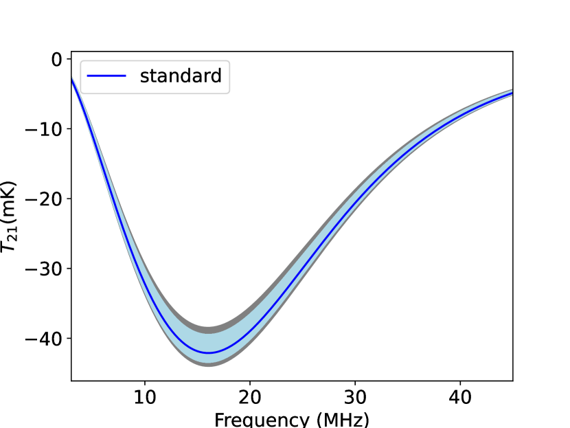
(a)

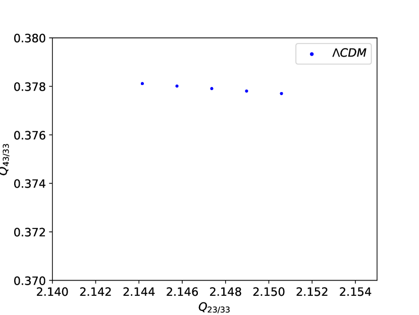
(b)

Figure 1: Left: Variation in $T_{21}$ with redshifted frequency upon varying cosmological parameters $(\Omega_{b},\Omega_{m},Y_{p},h)$ within $68\%$ CL [49], depicted by the grey band, whereas the solid blue line shows the $T_{21}$ signal for mean and the light blue band depicts the variation of $T_{21}^{\prime}$ (Eq. 11). Right: Shows variation in the consistency ratio $(Q_{i})$ corresponding to the grey band shown in the left figure.

The Universe was mostly homogeneous and isotropic during the Dark Ages in the absence of star formation. Thus, the Dark Ages 21-cm signal is independent of all astrophysical uncertainties which can be found during the cosmic dawn and reionization era. Thus, its future measurement may unveil pristine cosmological information, as discussed above. Along with the total signal, the shape of the signal in the frequency range $20\text{ MHz}\leq\nu\leq 45\text{ MHz}$ can provide valuable cosmological information.

Recently, authors in Ref. [9] have pointed out that $T_{21}$ shape is independent of cosmological parameters. Thereby, introducing an independent parameter, known as the “Dark Ages consistency ratio”, capable of testing the consistency of standard cosmology by distinguishing standard $T_{21}$ signal from any presence of the other type of exotic physics.

$$T_{21}^{\prime} = \frac{T_{21}}{\mathcal{M}(\phi)}\mathcal{M}(\phi^{\prime})$$ (11)

$$\mathcal{M}(\phi) = \frac{\left[\Omega_{b}h^{2}(1-Y_{p})\right]^{2}}{\sqrt{\Omega_{m}h^{2}}}$$ (12)

$$\mathcal{M}(\phi^{\prime}) = \mathcal{M}(\Omega_{m}^{\prime},\Omega_{b}^{\prime},h^{\prime},Y_{p}^{\prime})$$ (13)

$${Q}_{i/33}=\frac{T_{21}(\nu_{i})}{T_{21}(33\mbox{\ }\rm MHz)}$$ (14)

From Eq. (2), it is evident that $T_{21}$ depends primarily on cosmological parameters: $\Omega_{m}$, $\Omega_{b}$, $h$, and $Y_{p}$. Although their values are known accurately, still we vary them within $68\%$ CL to observe the variations in $T_{21}$ [49], depicted by grey color in Fig. (1(a)). From the figure, it can be seen that $T_{21}$ shape is almost independent of these cosmological parameters, especially in the frequency range $20\mbox{\ }\rm{MHz}<\nu<45\mbox{\ }\rm MHz$. To verify the dependency we scaled $T_{21}$ with $\mathcal{M}(\phi)$ (Eq. 12). We plot $T_{21}/\mathcal{M}(\phi)$ in Fig. (1(a)) depicted in lightblue color. We can see that the shape of $T_{21}/\mathcal{M}(\phi)$ remains almost unchanged.

The reason for considering $\mathcal{M}(\phi)$ can be easily found out from Eq. (2). As discussed earlier, $x_{c}$ become ineffective $(\ll 1)$ for $z\lesssim 69$ and it is $\propto\left[\Omega_{b}h^{2}(1-Y_{p})\right]$ thus for such redshift range $T_{21}\propto\mathcal{M}(\phi)$. To verify that in the frequency range of $20\text{ MHz}\leq\nu\leq 45\text{ MHz}$, we randomly selected a frequency to $33\,\rm MHz$ as a base frequency. Further, we calculated the ratio $Q_{i/33}$ (Eq. 14) which always take a certain definite value for $\Lambda\rm CDM$ model for a given frequency $\nu_{i}$ in the frequency range of $20\mbox{\ }\rm{MHz}<\nu<50\mbox{\ }\rm MHz$. After varying the cosmological parameters $h$, $\Omega_{b}$, $\Omega_{m}$, and $Y_{p}$ in their corresponding $68\%$ CL range, that is, $(0.6724-0.6808)$, $(0.0485-0.0491)$, $(0.3046-0.316)$, and $(0.216-0.28)$ respectively [49], for illustration, we take 625 combinations in the aforementioned range to generate different $T_{21}$ signals. In Fig. (1(b)) we show the $Q_{i/33}$ ratio corresponding to those 625 $T_{21}$ signals, shown in the grey band of Fig. (1(a)). It can be seen that $Q_{43}$ remains almost constant whereas $Q_{23}$ lies between $[2.144,2.152]$. The reason for this can be analysed easily from the fact that the ratio $Q_{23/33}$ strongly depends on $\left[x_{c}/(1+x_{c})\right]$. As explained earlier, $x_{c}\ll 1$ for $\nu\gtrsim 30\text{ MHz}$ therefore, $Q_{43}$ attains a constant value whereas $Q_{23}$ varies mildly.

Future 21-cm observations may consider any two frequencies to check the consistency of the signal. Thus, any deviation from this value will conclude the presence of non-standard physics during the Dark Ages. This motivated us to look at the possibility of the 21-cm signal shape being independent of cosmological uncertainties.

3 Primordial magnetic fields

After the recombination epoch, there are two processes through which the primordial magnetic field can transfer energy into the IGM— ambipolar diffusion and turbulent decay. Ambipolar diffusion is important when plasma is partially ionized, whereas non-linear effects can lead to turbulent decay [40]. In this work, we follow Sethi and Subramanian [40] to explain the energy dissipation by PMFs via ambipolar diffusion and turbulent decay into the IGM.

Before writing the expression for energy dissipation, it is important to explain the statistical properties of the primordial magnetic fields. We consider a statistically isotropic and homogeneous Gaussian field. Therefore, the statistical properties of PMFs can be determined by the power spectrum. Following Ref. [48], we consider the power spectrum $P_{B}(k)$ in $k$ modes as,

$$P_{B}(k)=\frac{B_{n}^{2}\ (2\pi)^{n_{B}+5}}{\Gamma\left[\left(n_{B}+3\right)/2\right]}\frac{k^{n_{B}}}{k_{n}^{n_{B}+3}}\,,$$ (15)

where, $B_{n}$ is the PMFs amplitude normalised at a length scale of $1\text{ Mpc}$, $\Gamma$ is the Gamma function, $k_{n}=2\pi\text{ Mpc}^{-1}$, and $n_{B}$ is the spectral index of PMFs. The magnetic field $B_{l}^{2}$ smoothed at any length scale $l$ can be expressed as [48, 29],

$$B_{l}^{2}=\int_{0}^{\infty}\frac{d^{3}k}{(2\pi)^{3}}e^{-k^{2}l^{2}}P_{B}(k)=B_{n}^{2}\left(k_{l}/k_{n}\right)^{n_{B}+3}\,.$$ (16)

It can be seen that for $n_{B}=-3.0$, PMFs become scale independent thus in this work we have considered $n_{B}\gtrsim-3.0$ and $B_{n}^{2}=B_{1\text{Mpc}}^{2}$. Radiative viscosit can damp the PMFs on a small length scale ($k>k_{c}$) before recombination [40, 63, 64]. Therefore, $P_{B}(k)$ vanishes on inverse length scales greater than the cut-off scale $k_{c}$, which can be expressed as follows.

$$P_{B}(k)=0\quad\forall~{}k\geq k_{c}$$ (17)

$$k_{n}^{2}=k_{c,i}^{2}\frac{V_{a}^{2}}{\sigma_{T}}\int_{0}^{1088}\frac{(1+z)dz}{n_{e}(z)}\,,$$ (18)

The expanding Universe makes the cut-off scale evolve over time as $k_{c}=g(z)k_{c,i}$ with $g(1088)=1$, where $k_{c,i}$ is the cut-off scale at $z=1088$, $g(z)$ determines temporal evolution of the cut-off scale, and $z=1088$ represents the end of the recombination epoch. Thus, Eq.(15) holds true for $k<k_{c}$. The $k_{c,i}$ can be expressed as Eq. (18) which can be approximated as follows [65].

$$k_{c,i}=k_{n}\left[1.32\times 10^{-3}B_{n}^{2}\left(\frac{0.02}{\Omega_{b}h^{2}}\right)\left(\frac{\Omega_{m}h^{2}}{0.15}\right)^{1/2}\right]^{-\frac{1}{(n_{B}+5)}}$$ (19)

In Eq. (18), $V_{a}^{2}=B_{n}(k_{c},z)/\left(4\pi\rho_{b}(z)\right)$ is the Alfvén wave velocity, $\sigma_{T}$ is the Thompson scattering cross-section, and $n_{e}$ is electron number density.

In the presence of magnetic fields, the Lorentz force will only act on the ionized component of the IGM. This force can accelerate the ionized components thereby increasing the relative velocity between neutral and ionized components. This enhanced relative velocity is damped via ion-neutral collisions in plasma draining the energy of the magnetic fields [40, 66]. This process is called ambipolar diffusion which is crucial in a nearly neutral molecular cloud [67]. In the early Universe, the neutral component of the IGM contained primarily hydrogen atoms and some fraction of Helium atom. Thus, we ignore the dissipation of energy into Helium and formulate the volume rate of energy transfer proportional to average Lorentz force squared as [68, 40],

$$\Gamma_{\rm ambi}=\frac{\rho_{\rm HI}}{\rho_{b}^{2}\rho_{i}}\frac{1}{16\pi^{2}\gamma_{e}}\big{|}\left(\vec{\nabla}\times\vec{B}\right)\times\vec{B}\big{|}^{2}$$ (20)

here, $\rho_{\rm HI}$, $\rho_{b}$ and $\rho_{i}$ are the energy densities of the neutral hydrogen atoms, total baryons and ions, respectively, present in the plasma. Here, $\gamma_{e}$ is the ion-neutral coupling coefficient, which can be approximated as $\gamma_{e}\approx 1.9\times 10^{14}\left(T_{g}/\rm K\right)^{0.375}\rm cm^{3}/g/s$ [40, 69]. $\rho_{\rm HI}/\rho_{i}\sim(1-x_{e})/x_{e}$ and $\rho_{b}\sim m_{H}n_{H}$, where $m_{H}$ and $n_{H}$ are mass of hydrogen atom and hydrogen number density in comoving coordinate, respectively. Therefore, now Eq. (20) can be written as [43],

$$\Gamma_{\rm ambi}=\frac{(1-x_{e})/x_{e}}{16\pi^{2}\gamma_{e}(m_{H}n_{H})^{2}}\big{|}\left(\vec{\nabla}\times\vec{B}\right)\times\vec{B}\big{|}^{2}$$ (21)

Now, by substituting Eq. (15), we can calculate $\vec{L}=(\vec{\nabla}\times\vec{B})\times\vec{B}$ at redshift $z$ as,

$$\big{|}\vec{L}\big{|}^{2}=\int\int\frac{d^{3}k_{1}d^{3}k_{2}}{(2\pi)^{6}}k_{1}^{2}P_{B}(k_{1})P_{B}(k_{2})g^{2n_{B}+8}(z)(1+z)^{10}$$ (22)

It should be noted that the derivative operator in the Lorentz force $\vec{L}$ is taken with respect to proper coordinate and $B\sim B_{n}(1+z)^{2}$ where $B_{n}$ is the present-day magnetic field strength, thus $\vec{L}\propto(1+z)^{5}$. After the decoupling of IGM from CMB, $T_{g}$ fell $\propto(1+z)$ till $z\sim 300$ and soon after that it fell $\propto(1+z)^{2}$, which brings us to notice that $\Gamma_{\rm ambi}\propto(1+z)^{3.63}\,(1-x_{e})/x_{e}$ for $z\gtrsim 300$ and $\propto(1+z)^{3.25}/x_{e}$ otherwise [70].

Before recombination, turbulent motion in plasma is highly damped due to large radiative viscosity. However, the damping lowers down after recombination which leads to the transfer of energy to small scales from non-linear interaction dissipating the magnetic field on larger scales— known as turbulence decay [71]. In the matter-dominated epoch, the approximate decay rate for a non-helical field is given by [40],

$$\Gamma_{\rm decay}=\frac{3\,q_{B}\,E_{B}\,H(z)}{2}\frac{[\ln(1+t_{d}/t_{\rm rec})]^{q_{B}}}{\left[\ln(1+t_{d}/t_{\rm rec})+\ln(t/t_{\rm rec})\right]^{1+q_{B}}}$$ (23)

where, $q_{B}=2(n_{B}+3)/(n_{B}+5)$, $t_{d}=1/\left(k_{c}V_{a}\right)$ for $n_{B}>-3.0$ represents Alfvén time scale for cut-off scale [40], $t_{\rm rec}=2/(3H)$ is recombination time-period, and $E_{B}=B^{2}/8\pi$ is the magnetic energy. Similar to Eq. (22), now $E_{B}$ in terms of $g(z)$ can be calculated as,

$$E_{B}=\frac{1}{8\pi}\int\frac{d^{3}k}{(2\pi)^{3}}P_{B}(k)g^{n_{B}+3}(z)(1+z)^{4}\,,$$ (24)

The evolution of $k_{c}$, as discussed above, is defined by $g(z)$. Therefore, the evolution of $g(z)$ can be found by substituting Eq. (21), Eq. (22), Eq. (23), Eq. (24) in the below equation representing conservation of magnetic energy [70].

$$\frac{dE_{B}}{dz}=4\frac{E_{B}}{1+z}+\frac{1}{(1+z)H(z)}\left(\Gamma_{\rm decay}+\Gamma_{\rm ambi}\right)$$ (25)

4 Thermal evolution of IGM in PMFs

The evolution of the kinetic temperature of IGM $(T_{g})$ and the ionization fraction $(x_{i}\approx x_{e})$ with redshift in the absence of any exotic source of energy injection can be expressed as follows

$$\frac{dx_{e}}{dz}=\frac{\mathcal{P}}{(1+z)H}\left[n_{H}x_{e}^{2}\alpha_{B}-(1-x_{e})\beta_{B}e^{-E_{\alpha}/T_{\gamma}}\right]$$ (26)

$$\mathcal{P}=\frac{1+\mathcal{K}_{H}\Lambda_{H}n_{H}(1-x_{e})}{1+\mathcal{K}_{H}(\Lambda_{H}+\beta_{H})n_{H}(1-x_{e})}$$ (27)

$$\frac{dT_{g}}{dz}=2\frac{Tg}{1+z}+\frac{\Gamma_{c}}{(1+z)H}\left(T_{g}-T_{\gamma}\right)$$ (28)

In Eq. (26), $\mathcal{P}$ is Peebles coefficient [72, 73], while $\alpha_{B}$ and $\beta_{B}$ are the case-B recombination and photo-ionization rates, respectively [74, 75, 76]. $\mathcal{K}_{H}=\pi^{2}/(E_{\alpha}^{3}H)$, $E_{\alpha}=10.2\,\rm eV$, and $\Lambda_{H}=8.22/\text{sec}$ in Eq. (27) represents redshifting of Ly${\alpha}$ photons, rest frame energy of Ly$\alpha$ photon, and 2S-1S level two-photon decay rate in hydrogen atom respectively [77]. The first term of Eq. (28) represents adiabatic cooling of IGM and the second term represents the coupling between CMB and IGM due to inverse-Compton scattering [78]. The Compton scattering rate $(\Gamma_{c})$ can be defined as,

$$\Gamma_{c}=\frac{8n_{e}\sigma_{T}a_{r}T_{\gamma}^{4}(z)}{3m_{e}n_{\text{tot}}}$$ (29)

where, $m_{e}$, $\sigma_{T}$, and $f_{He}=0.08$ represent the mass of an electron, Thomson scattering cross-section, and Helium fraction, respectively. Whereas, $a_{r}=7.57\times 10^{-16}$ J $\text{m}^{-3}\,\text{K}^{-4}$ represents the radiation density constant, $n_{\rm tot}=n_{H}(1+f_{He}+x_{e})$ represents the total number density of gas, and the CMB temperature is represented by $T_{\gamma}(z)=T_{0}(1+z)$ where $T_{0}=2.725\rm K$ [74, 75].

The primordial magnetic fields cannot ionize the IGM directly, instead, it heats the IGM via ambipolar diffusion (Eq. 21) and turbulent decay (Eq. 23) thereby ionizing it via collision mechanism. Therefore, in the presence of PMFs, Eq. (26) remains the same whereas, Eq. (28) can be written as follows, which we use to evaluate the thermal evolution of IGM in the presence of PMFs,

$$\frac{dT_{g}}{dz}=2\frac{Tg}{1+z}+\frac{\Gamma_{c}}{(1+z)H}\left(T_{g}-T_{\gamma}\right)+\frac{2}{3n_{\rm tot}(1+z)H(z)}\left(\Gamma_{\rm ambi}+\Gamma_{\rm decay}\right)$$ (30)

5 Results and Discussions

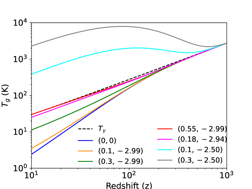
(a)

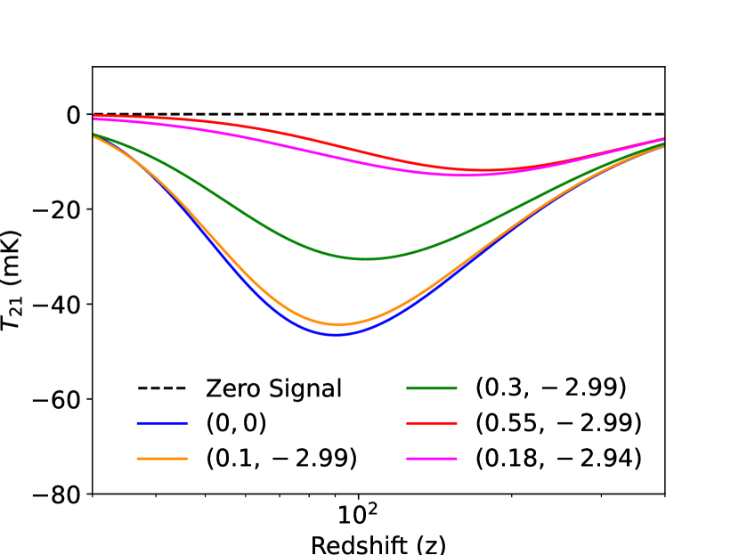
(b)

Figure 2: Left: The thermal evolution IGM with redshift. The black dashed line represents CMB temperature $(T_{\gamma})$, and the blue solid line represents standard IGM temperature evolution. Other solid lines represent the IGM evolution in the presence of PMFs with different $(B_{n}/\text{nG},n_{B})$. Right: The Dark Ages global 21-cm signal with redshift in the presence and absence of PMFs. The blue solid curve depicted by $(0,0)$ shows the standard global 21-cm signal. The black dashed line represents zero or non-existence of a signal whereas other solid lines represent the presence of PMFs for different $(B_{n}/\text{nG},n_{B})$.

To evaluate the thermal evolution of IGM in the presence of PMFs, we calculated the average squared Lorentz force in Eq. (21) from Eq. (22) and magnetic energy $(E_{B})$ from Eq. (24). By substituting Eq. (21), Eq. (23), and Eq. (24) in Eq. (25) we determined $dg(z)/dz$ with the initial condition $g(1088)=1$ [48]. Consequently, Eq. (25) provide the evolution of cut-off scale $(k_{c})$ over redshift. Subsequently, the thermal evolution of IGM over redshift is achieved by simultaneously solving Eq. (25), Eq. (26), and Eq. (30) with the initial condition of $T_{g}=2967.6\text{ K}$ and $x_{e}=0.1315$ at redshift $z=1088$ taken from Recfast++ [79, 80].

From Fig. (2(a)), we can see that $T_{\gamma}$ evolves $\propto(1+z)$ whereas $T_{g}$ evolves $\propto(1+z)^{2}$ in the absence of PMFs, representing standard cosmological scenario— depicted by the black dashed and blue solid lines respectively. However, after the inclusion of PMFs, the temperature of the IGM starts to increase, as shown by the orange solid line corresponding to $B_{n}=0.1\text{ nG}$ and $n_{B}=-2.99$. To examine further effects of the magnetic field on IGM, we gradually increased the strength of $B_{n}$ while keeping the spectral index $(n_{B})$ fixed to $-2.99$. We observed an increase in the IGM heating, eventually reaching $T_{\gamma}$— depicted by the solid orange, green, and red lines, where, we increased $B_{n}$ from $0.1-0.55\,\rm nG$, respectively. It should be noted that, despite increasing the magnetic field strength $(B_{n})$, the redshift of decoupling remained almost unaffected. However, increasing $n_{B}$ from $-2.99$ to $-2.50$ resulted in an early heating of IGM, $z\sim 945$. This has been shown by the cyan and grey solid lines, where $n_{B}$ is $-2.50$ while $B_{n}$ are $0.1$ nG and $0.3$ nG respectively. In a comparison of the orange and green solid lines, where $n_{B}=-2.99$, the significant heating due to change in $n_{B}$ can be observed. Furthermore, we plotted IGM evolution for $B_{n}=0.18\,\rm nG$ and $n_{B}=-2.94$, shown by the magenta solid line. Next, we discuss the effects of magnetic field strength and spectral index on the IGM evolution.

As discussed earlier in Sec. (3), $\Gamma_{\rm ambi}$ varies $\propto(1+z)^{3.625}$ for $z\gtrsim 300$, and $\propto(1+z)^{3.25}$ otherwise. Furthermore by analysing Eq. (15) and Eq. (22), the dependency on $n_{B}$ and $B_{n}$ can be found as follow $\left(\Gamma\left[(n_{B}+3)/2\right]\right)^{-2}$ and $B_{n}^{4}$, respectively. From Eq. (23) it can be seen that, upon ignoring the logarithmic terms, the variation of $\Gamma_{\rm decay}$ follows $(1+z)^{5.5}$. Similarly from Eq. (24), the dependency of the magnetic energy density on $n_{B}$ and $B_{n}$ can be found as follows $\left(\Gamma\left[(n_{B}+3)/2\right]\right)^{-1}$ and $B_{n}^{2}$, respectively. Thus, for a fixed $n_{B}$ and $B_{n}$, the heating of IGM in the presence of PMFs is dominated by turbulent decay over high redshifts compared to the ambipolar diffusion dominating the lower redshift regime. In addition, the quantified dependency of $\Gamma_{\rm decay}$ and $\Gamma_{\rm ambi}$ on $n_{B}$ for a fixed $B_{n}$ and $z$ can be analysed by calculating $\Gamma[(n_{B}+3)/2]$. For example, $\Gamma[(n_{B}+3)/2]$ takes a value of $2.5\times 10^{-5}$, $9.3\times 10^{-4}$, and $0.076$ for $n_{B}$ equals to $-2.99$, $-2.94$, and $-2.5$, respectively. Therefore, a small change in $n_{B}$ can lead to a huge difference in the dissipation of magnetic energy. The higher value of $n_{B}$ enhances the dissipation of magnetic fields resulting in a rapid draining of magnetic energy $(E_{B})$. Hence, after a certain redshift, the magnetic heating gradually becomes small thereby making the IGM following $\propto(1+z)^{2}$ due to adiabatic expansion. The same has been shown by the cyan and grey solid lines in Fig. (2(a)), where we have fixed $n_{B}$ to $-2.50$ while varying $B_{n}$ from $0.1$ to $0.5\,\rm nG$. It can seen that both dissipate magnetic energy efficiently into the IGM till a redshift $\sim 122$ and $\sim 85$, respectively, and decline afterwards making the IGM temperature fall due to adiabatic expansion. However, a higher $B_{n}$ is capable of dissipating energy for a longer time due to the availability of magnetic energy $(E_{B})$.

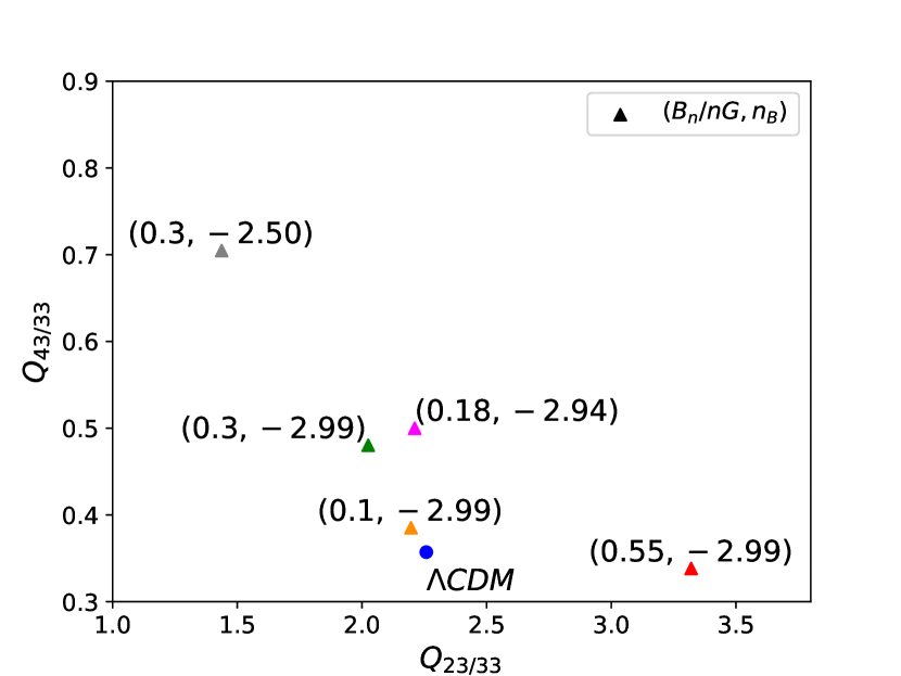
(a)

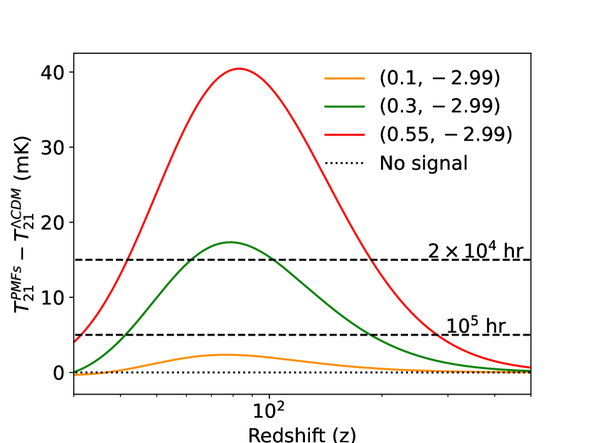
(b)

Figure 3: Left: Shows the consistency ratio (Eq. 14) for different $(B_{n}/\text{nG},n_{B})$ values plotted as $Q_{43}$ and $Q_{23}$ with the reference frequency $\nu_{i}=33\text{ MHz}$. Right: Shows the difference between the 21-cm signal for the $\Lambda$CDM model and the scenarios including primordial magnetic fields. The black-dashed line represents uncertainties in the Dark Ages $T_{21}$ signal with integration time of observation. For an integration time of 20,000 and $10^{5}$ hours, the uncertainty in the detection of the standard $T_{21}$ signal becomes 15 mK and 5 mK, respectively [81, 82]. Thus, the green and red curves can be measured with an integration time of less than 20,000 hours which represents PMFs with spectral index fixed at $-2.99$ while $B_{n}/\text{nG}$ equals 0.3 and 0.5 respectively.

To study the effects of PMFs on the Dark Ages $T_{21}$ signal we evaluated Eq. (2) and Eq. (4), and plotted $T_{21}$ for different $(B_{n}/\text{nG},n_{B})$ values. In Fig. (2(b)), the black dashed lines depict $T_{21}=0$ mK representing the non-existence of the Dark Ages 21-cm signal. To begin with, we studied the evolution of $T_{21}$ over the frequency in the absence of PMFs representing the standard cosmological scenarios which has been shown by the blue solid line. Furthermore, to study the effect of primordial magnetic fields, we increase $B_{n}$ gradually as: 0, 0.1, 0.3 and $0.55\,\rm nG$— represented by blue, orange, green and red solid lines, respectively. As the IGM gets heated due to PMFs, the absorption peak of $T_{21}$ becomes smaller. It happens because the ratio $(T_{\gamma}/T_{g})$ reaches toward unity. We need to point out that, the values of $(B_{n}/\text{nG},n_{B})$ are nearly degenerated, which has been shown by the red and magenta solid line representing different values of magnetic field and spectral index and having almost similar $T_{21}$ features. The magnetic field strength for the magenta line is smaller than the red line but, we see nearly the same absorption in both lines— because it is compensated by a larger spectral index. In the present study, we constrain the parameter space $(B_{n}/\text{nG},n_{B})$ such that $T_{g}\simeq T_{\gamma}$— depicting a wiping out of the Dark Ages $T_{21}$ signal in the redshift $z\lesssim 89$. In the next paragraph, we discuss the consistency ratio.

We also study the consistency ratio $(Q_{i/33})$ shown in equation (14), for different magnetic field strength $(B_{n})$ and spectral index $(n_{B})$. We followed the definition of the consistency ratio provided in Ref. [9]. The authors have considered the reference frequency, $\nu_{i}=30\,\rm MHz$ while calculating $Q$ at frequencies of $40\,\rm MHz$ and $20\,\rm MHz$. Here, the frequency can be mapped with redshift as $\nu=1420/(1+z)\,\rm MHz$. The authors have shown that the ratio for a standard scenario attains nearly a constant value while plotting $Q_{40/30}$ vs $Q_{20/30}$, and the existence of an additional IGM heating can be distinguished clearly from the standard $\Lambda$CDM scenario. In Fig. (3(a)), we show the values of $Q_{i/33}$, where we calculated $Q$ values at $43\,\rm MHz$ and $23\,\rm MHz$ while taking $33\,\rm MHz$ as the base frequency. All the $Q$ values for different $(B_{n}/\rm nG,n_{B})$ acquire different places compared to the standard scenario depicted by the blue dot. Therefore, as suggested by the authors in Ref. [9], the “dark-ages consistency ratio” can be used by future experiments to check the consistency in their early stages of observations, where one requires the observation of $T_{21}$ at just three different frequencies to distinguish the non-standard IGM evolution from $\Lambda$CDM scenario.

Before we discuss the results of the present study, we need to check the detectability of the Dark Ages 21-cm signal. Future lunar-based experiments [81, 82], are capable of detecting $T_{21}$ at redshift $z\sim 89$ with $68\%$ CL $\left(\Delta T_{21}\sim 5\text{ mK}\right)$ in an integration time of $10^{5}$ hours. Where, $\Delta T_{21}$ is the deviation of detected $T_{21}$ from the standard $T_{21}$ signal. However, from Fig. (1(a)) it can seen that cosmological parameter uncertainty can vary the $T_{21}$ signal about 6 mK (grey band) at a frequency of $15.78$ MHz— the corresponding redshift is about 89. The mean value of $T_{21}$ at $15.78$ MHz is $-42\,\rm mK$ while the upper and lower values correspond to $-38\,\rm mK$ and $-44\,\rm mK$, respectively. Therefore, any observation of $T_{21}$ out of the grey band will indicate a new physics for the cosmological evolution. Therefore, we require the accuracy of $T_{21}$ observations to be greater than $\sim 6\,\rm mK$ to conclude the existence of beyond $\Lambda$CDM physics. In Fig. (3(b)), we have represented the same. The black dotted line represents no signal, whereas the two black dashed lines represent a variation in $T_{21}$ standard signal by $15\,\rm mK$ and $5\,\rm mK$ corresponding to 20,000 hours and $10^{5}$ hours of integration times, respectively for future lunar and space-based telescope [81, 82]. Recently in Ref. [8], the authors discuss the significance of the detection time of the standard Dark Ages global $T_{21}$ signal from a zero signal, to be $4.12\sigma$ and $41.2\sigma$ for an integration time of $10^{3}$ hours and $10^{5}$ hours respectively. Therefore, detecting and constraining PMFs having magnetic field strength and spectral index corresponding to $(0.1\text{ nG},-2.99)$, represented by the orange solid line, requires a well-calibrated instrument with detection of an uncertainty $<5\text{ mK}$. However, detecting a $(0.3\text{ nG},-2.99)$, depicted by the green solid line, can be achieved with an integration time of $10^{5}$ hours. Furthermore, the case with $(0.55\text{ nG},-2.99)$ depicted by the red solid line, can be difficult to observe. Therefore, the magnetic field strengths and spectral indexes which can heat the gas such that $T_{21}=0$ at $z\sim 89$, can be constrained with $10^{3}$ hours of integration time.

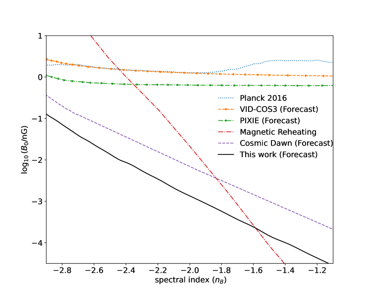
Figure 4: The upper bound on the present-day strength of primordial magnetic fields as a function of spectral index. The red dash-dotted and the blue dashed lines show existing constraints from Planck 2016 and the magnetic reheating process before CMB spectral distortion ($z\gtrsim 2\times 10^{6}$), respectively [35, 38]. In addition, we have also plotted some forecasting constraints by future experiments, such as PIXIE (green dot-dashed line)[37] and VID-COS3 line intensity measurement (orange dot-dashed line)[83]. The purple dashed line depicts the bound by considering $T_{21}\sim 0$ during the cosmic dawn [48]. The black solid line shows the bounds from the present work.

To get the upper bounds on the present-day strength of primordial magnetic fields in $(B_{n}/\text{nG},n_{B})$ plane, we consider that $T_{21}\simeq 0$ at $z=89$. In addition to this, we also check that the combination $(B_{n}/\text{nG},n_{B})$ do not give an emission signal during the cosmic dawn ($z\sim 17$). In a previous article [48], authors constrain the parameter space $(B_{n}/\text{nG},n_{B})$ such that $T_{g}\leq T_{\gamma}$ at $z_{\rm abs}=17$— shown by purple dashed line in Fig. (4). It is to be noted that, in this article, the authors consider that the gas temperature is completely coupled to the spin temperature— $T_{s}\sim T_{g}$. In Fig. (4), we have shown the existing and possible future bounds on $(B_{n}/\text{nG},n_{B})$. The red dash-dotted line represents the upper bound on the present-day strength of PMFs as a function of spectral index by considering the “magnetic reheating” of plasma before CMB spectral distortion era [38]. Here, “magnetic reheating” is a process which changes the baryon-to-photon number ratio by dissipating the magnetic fields. The blue dotted line depicts the bound from Planck 2016 [35]. In addition to these bounds, we have also shown some forecast bounds from future experiments– PIXIE (green dot-dashed line) and VID-COS3 (orange dot-dashed line) [37, 83]. The black solid line represents the bound from this paper. We found that for the nearly scale-invariant spectral index, $-2.99$, the present-day strength of PMFs should be smaller than $0.55\,\rm nG$. For the spectral index of $-2.5$, $-2.0$, $-1.5$ and $-1.0$ the upper limits on $B_{0}$ are $2.2\times 10^{-2}$, $2.1\times 10^{-3}$, $2.0\times 10^{-4}$ and $2.5\times 10^{-5}\,\rm nG$, respectively. As we increase the spectral index the bounds get stronger. As discussed earlier, increasing the spectral index increases the magnetic heating of IGM. Therefore, to get the desired gas temperature we have to reduce the value of $B_{0}$ when we increase the spectral index. The obtained bound can be summarised approximately by the following equation,

$$\log_{10}\left({B_{n}}/{\text{nG}}\right)\lesssim-\left(2n_{B}+1.2\right)\,.$$ (31)

6 Summary and Conclusion

In this work, we have studied the effect of primordial magnetic fields (PMFs) on the Dark Ages global 21-cm signal $(T_{21})$. Primordial magnetic fields can dissipate energy into IGM via ambipolar diffusion (Eq. 21) and turbulent decay (Eq. 23) after recombination. The Dark Ages 21-cm signal being independent of astrophysical uncertainty can help identify the existence of any non-standard physics. Recently proposed experiments, such as FARSIDE [3], DAPPER [4], SEAMS [5], LuSee Night [6], might be able to measure the $T_{21}$ during the Dark Ages in the near future.

To begin with, we studied the implications of cosmological parameter uncertainties on the $T_{21}$ signal. We varied the cosmological parameter $\Omega_{m},\Omega_{b},Y_{p}$, and $h$ within their corresponding $68\%$ CL, and found a total variation in 21-cm signal to be $\sim 6\,\rm mK$ at $z\simeq 89$. Furthermore, we have also studied the Dark Ages consistency ratio as defined in Ref. [9]. Using this technique, we can identify the presence of any non-standard exotic source of IGM heating by observing the global 21-cm signal at only three different frequencies during the Dark Ages. Further, in Fig (3(a)), we have shown the possibility of detecting PMFs parameter space using the Dark Ages consistency ratio. Finally, in Fig (4), we have shown the upper bound on the preset-day strength of PMFs as a function of the spectral index. We would also like to note that, our constraints are stronger compared to Planck 2016 [35] and bounds obtained from magnetic reheating prior to CMB spectral distortion for some parameter space ($n_{B}\lesssim-1.58$) [38].

References

- \bibcommenthead
- Pritchard and Loeb [2012] Pritchard, J.R., Loeb, A.: 21-cm cosmology. Rept. Prog. Phys. 75, 086901 (2012) https://doi.org/10.1088/0034-4885/75/8/086901 arXiv:1109.6012 [astro-ph.CO]
- Monsalve et al. [2023] Monsalve, R.A., et al.: Mapper of the IGM Spin Temperature (MIST): Instrument Overview (2023) arXiv:2309.02996 [astro-ph.IM]
- Burns et al. [2019] Burns, J., Hallinan, G., Lux, J., Romero-Wolf, A., Teitelbaum, L., Chang, T.-C., Kocz, J., Bowman, J., MacDowall, R., Kasper, J., Bradley, R., Anderson, M., Rapetti, D.: FARSIDE: A Low Radio Frequency Interferometric Array on the Lunar Farside. In: Bulletin of the American Astronomical Society, vol. 51, p. 178 (2019). https://doi.org/10.48550/arXiv.1907.05407
- Burns et al. [2021] Burns, J., Bale, S., Bradley, R., Ahmed, Z., Allen, S.W., Bowman, J., Furlanetto, S., MacDowall, R., Mirocha, J., Nhan, B., Pivovaroff, M., Pulupa, M., Rapetti, D., Slosar, A., Tauscher, K.: Global 21-cm Cosmology from the Farside of the Moon. arXiv e-prints, 2103–05085 (2021) https://doi.org/10.48550/arXiv.2103.05085 arXiv:2103.05085 [astro-ph.CO]
- Borade et al. [2021] Borade, R., George, G.N., Gharpure, D.C.: FPGA based data acquisition and processing system for space electric and magnetic sensors (SEAMS). AIP Conference Proceedings 2335(1), 030005 (2021) https://doi.org/10.1063/5.0043435
- Bale et al. [2023] Bale, S.D., Bassett, N., Burns, J.O., Dorigo Jones, J., Goetz, K., Hellum-Bye, C., Hermann, S., Hibbard, J., Maksimovic, M., McLean, R., Monsalve, R., O’Connor, P., Parsons, A., Pulupa, M., Pund, R., Rapetti, D., Rotermund, K.M., Saliwanchik, B., Slosar, A., Sundkvist, D., Suzuki, A.: LuSEE ’Night’: The Lunar Surface Electromagnetics Experiment. arXiv e-prints, 2301–10345 (2023) https://doi.org/10.48550/arXiv.2301.10345 arXiv:2301.10345 [astro-ph.IM]
- Mondal and Barkana [2023] Mondal, R., Barkana, R.: Prospects for precision cosmology with the 21 cm signal from the dark ages. Nature Astronomy 7, 1025–1030 (2023) https://doi.org/10.1038/s41550-023-02057-y arXiv:2305.08593 [astro-ph.CO]
- Mondal et al. [2024] Mondal, R., Barkana, R., Fialkov, A.: Constraining exotic dark matter models with the dark ages 21-cm signal. Mon. Not. Roy. Astron. Soc. 527(1), 1461–1471 (2024) https://doi.org/10.1093/mnras/stad3317 arXiv:2310.15530 [astro-ph.CO]
- Okamatsu et al. [2023] Okamatsu, F., Minoda, T., Takahashi, T., Yamauchi, D., Yoshiura, S.: Dark age consistency in the 21cm global signal (2023) arXiv:2309.06762 [astro-ph.CO]
- Bowman et al. [2018] Bowman, J.D., Rogers, A.E.E., Monsalve, R.A., Mozdzen, T.J., Mahesh, N.: An absorption profile centred at 78 megahertz in the sky-averaged spectrum. Nature 555(7694), 67–70 (2018) https://doi.org/10.1038/nature25792 arXiv:1810.05912 [astro-ph.CO]
- Singh et al. [2022] Singh, S., Nambissan T., J., Subrahmanyan, R., Udaya Shankar, N., Girish, B.S., Raghunathan, A., Somashekar, R., Srivani, K.S., Sathyanarayana Rao, M.: On the detection of a cosmic dawn signal in the radio background. Nature Astron. 6(5), 607–617 (2022) https://doi.org/10.1038/s41550-022-01610-5 arXiv:2112.06778 [astro-ph.CO]
- DeBoer et al. [2017] DeBoer, D.R., et al.: Hydrogen Epoch of Reionization Array (HERA). Publ. Astron. Soc. Pac. 129(974), 045001 (2017) https://doi.org/10.1088/1538-3873/129/974/045001 arXiv:1606.07473 [astro-ph.IM]
- de Lera Acedo et al. [2022] Lera Acedo, E., et al.: The REACH radiometer for detecting the 21-cm hydrogen signal from redshift z 7.5–28. Nature Astron. 6(7), 998 (2022) https://doi.org/10.1038/s41550-022-01817-6 arXiv:2210.07409 [astro-ph.CO]
- Tiwari et al. [2023] Tiwari, H., McKinley, B., Trott, C.M., Thyagarajan, N.: Measuring the global 21-cm signal with the MWA-II: improved characterisation of lunar-reflected radio frequency interference. Publ. Astron. Soc. Austral. 40, 055 (2023) https://doi.org/10.1017/pasa.2023.57 arXiv:2306.01013 [astro-ph.IM]
- Barkana et al. [2018] Barkana, R., Outmezguine, N.J., Redigolo, D., Volansky, T.: Strong constraints on light dark matter interpretation of the EDGES signal. Phys. Rev. D 98(10), 103005 (2018) https://doi.org/%****␣sn-article.bbl␣Line␣325␣****10.1103/PhysRevD.98.103005 arXiv:1803.03091 [hep-ph]
- Fialkov et al. [2018] Fialkov, A., Barkana, R., Cohen, A.: Constraining Baryon–Dark Matter Scattering with the Cosmic Dawn 21-cm Signal. Phys. Rev. Lett. 121, 011101 (2018) https://doi.org/10.1103/PhysRevLett.121.011101 arXiv:1802.10577 [astro-ph.CO]
- Feng and Holder [2018] Feng, C., Holder, G.: Enhanced global signal of neutral hydrogen due to excess radiation at cosmic dawn. Astrophys. J. Lett. 858(2), 17 (2018) https://doi.org/10.3847/2041-8213/aac0fe arXiv:1802.07432 [astro-ph.CO]
- Lawson and Zhitnitsky [2019] Lawson, K., Zhitnitsky, A.R.: The 21 cm absorption line and the axion quark nugget dark matter model. Phys. Dark Univ. 24, 100295 (2019) https://doi.org/10.1016/j.dark.2019.100295 arXiv:1804.07340 [hep-ph]
- Lawson and Zhitnitsky [2013] Lawson, K., Zhitnitsky, A.R.: Isotropic Radio Background from Quark Nugget Dark Matter. Phys. Lett. B 724, 17–21 (2013) https://doi.org/10.1016/j.physletb.2013.05.070 arXiv:1210.2400 [astro-ph.CO]
- Pospelov et al. [2018] Pospelov, M., Pradler, J., Ruderman, J.T., Urbano, A.: Room for New Physics in the Rayleigh-Jeans Tail of the Cosmic Microwave Background. Phys. Rev. Lett. 121(3), 031103 (2018) https://doi.org/10.1103/PhysRevLett.121.031103 arXiv:1803.07048 [hep-ph]
- Bhatt et al. [2020] Bhatt, J.R., Natwariya, P.K., Nayak, A.C., Pandey, A.K.: Baryon-Dark matter interaction in presence of magnetic fields in light of EDGES signal. Eur. Phys. J. C 80(4), 334 (2020) https://doi.org/10.1140/epjc/s10052-020-7886-x arXiv:1905.13486 [astro-ph.CO]
- Natwariya and Nayak [2022] Natwariya, P.K., Nayak, A.C.: Bounds on sterile neutrino lifetime and mixing angle with active neutrinos by global 21 cm signal. Phys. Lett. B 827, 136955 (2022) https://doi.org/10.1016/j.physletb.2022.136955 arXiv:2202.06007 [hep-ph]
- Natwariya et al. [2021] Natwariya, P.K., Nayak, A.C., Srivastava, T.: Constraining spinning primordial black holes with global 21-cm signal. Mon. Not. Roy. Astron. Soc. 510, 4236 (2021) https://doi.org/10.1093/mnras/stab3754 arXiv:2107.12358 [astro-ph.CO]
- Saha and Laha [2022] Saha, A.K., Laha, R.: Sensitivities on nonspinning and spinning primordial black hole dark matter with global 21-cm troughs. Phys. Rev. D 105(10), 103026 (2022) https://doi.org/%****␣sn-article.bbl␣Line␣475␣****10.1103/PhysRevD.105.103026 arXiv:2112.10794 [astro-ph.CO]
- Carilli and Taylor [2002] Carilli, C.L., Taylor, G.B.: Cluster Magnetic Fields. Ann. Rev. Astron. Astrophys. 40, 319–348 (2002) https://doi.org/10.1146/annurev.astro.40.060401.093852 arXiv:astro-ph/0110655 [astro-ph]
- Vacca et al. [2018] Vacca, V., et al.: Observations of a nearby filament of galaxy clusters with the Sardinia Radio Telescope. Mon. Not. Roy. Astron. Soc. 479(1), 776–806 (2018) https://doi.org/10.1093/mnras/sty1151 arXiv:1804.09199 [astro-ph.CO]
- Neronov and Vovk [2010] Neronov, A., Vovk, I.: Evidence for strong extragalactic magnetic fields from Fermi observations of TeV blazars. Science 328, 73–75 (2010) https://doi.org/10.1126/science.1184192 arXiv:1006.3504 [astro-ph.HE]
- Vovk et al. [2012] Vovk, I., Taylor, A.M., Semikoz, D., Neronov, A.: Fermi/LAT observations of 1ES 0229+200: implications for extragalactic magnetic fields and background light. Astrophys. J. Lett. 747, 14 (2012) https://doi.org/10.1088/2041-8205/747/1/L14 arXiv:1112.2534 [astro-ph.CO]
- Natwariya [2022] Natwariya, P.K.: 21 cm Line Astronomy and Constraining New Physics. PhD thesis, Indian Inst. Tech., Gandhinagar (2022)
- Turner and Widrow [1988] Turner, M.S., Widrow, L.M.: Inflation-produced, large-scale magnetic fields. Phys. Rev. D. 37(10), 2743–2754 (1988) https://doi.org/10.1103/PhysRevD.37.2743
- Ratra [1992] Ratra, B.: Cosmological “Seed” Magnetic Field from Inflation. Astrophys. J. Lett. 391, 1 (1992) https://doi.org/10.1086/186384
- Bassett et al. [2001] Bassett, B.A., Pollifrone, G., Tsujikawa, S., Viniegra, F.: Preheating-cosmic magnetic dynamo? Phys. Rev. D. 63(10), 103515 (2001) https://doi.org/10.1103/PhysRevD.63.103515 arXiv:astro-ph/0010628 [astro-ph]
- Sicotte [1997] Sicotte, H.: Large-scale magnetic fields in texture-seeded cosmological models. Mon. Not. Roy. Astron. Soc. 287(1), 1–9 (1997) https://doi.org/10.1093/mnras/287.1.1
- Hutschenreuter et al. [2018] Hutschenreuter, S., Dorn, S., Jasche, J., Vazza, F., Paoletti, D., Lavaux, G., Enßlin, T.A.: The primordial magnetic field in our cosmic backyard. Classical and Quantum Gravity 35(15), 154001 (2018) https://doi.org/10.1088/1361-6382/aacde0 arXiv:1803.02629 [astro-ph.CO]
- Planck Collaboration et al. [2016] Planck Collaboration, et al.: Planck 2015 results - xix. constraints on primordial magnetic fields. Astron. Astrophys. 594, 19 (2016) https://doi.org/10.1051/0004-6361/201525821
- Zucca et al. [2017] Zucca, A., Li, Y., Pogosian, L.: Constraints on primordial magnetic fields from Planck data combined with the South Pole Telescope CMB B -mode polarization measurements. Phys. Rev. D. 95(6), 063506 (2017) https://doi.org/10.1103/PhysRevD.95.063506 arXiv:1611.00757 [astro-ph.CO]
- Kunze and Komatsu [2014] Kunze, K.E., Komatsu, E.: Constraining primordial magnetic fields with distortions of the black-body spectrum of the cosmic microwave background: pre- and post-decoupling contributions. JCAP 2014(1), 009 (2014) https://doi.org/10.1088/1475-7516/2014/01/009 arXiv:1309.7994 [astro-ph.CO]
- Saga et al. [2017] Saga, S., Tashiro, H., Yokoyama, S.: Magnetic reheating. Monthly Notices of the Royal Astronomical Society: Letters 474(1), 52–55 (2017) https://doi.org/10.1093/mnrasl/slx195
- Minoda et al. [2017] Minoda, T., Hasegawa, K., Tashiro, H., Ichiki, K., Sugiyama, N.: Thermal Sunyaev-Zel’dovich effect in the intergalactic medium with primordial magnetic fields. Phys. Rev. D. 96(12), 123525 (2017) https://doi.org/10.1103/PhysRevD.96.123525 arXiv:1705.10054 [astro-ph.CO]
- Sethi and Subramanian [2005] Sethi, S.K., Subramanian, K.: Primordial magnetic fields in the post-recombination era and early reionization. Mon. Not. Roy. Astron. Soc. 356(2), 778–788 (2005) https://doi.org/10.1111/j.1365-2966.2004.08520.x arXiv:astro-ph/0405413 [astro-ph]
- Tashiro and Sugiyama [2006] Tashiro, H., Sugiyama, N.: Probing primordial magnetic fields with the 21-cm fluctuations. Mon. Not. Roy. Astron. Soc. 372(3), 1060–1068 (2006) https://doi.org/10.1111/j.1365-2966.2006.10901.x arXiv:astro-ph/0607169 [astro-ph]
- Jedamzik and Pogosian [2020] Jedamzik, K., Pogosian, L.: Relieving the Hubble tension with primordial magnetic fields. Phys. Rev. Lett. 125(18), 181302 (2020) https://doi.org/10.1103/PhysRevLett.125.181302 arXiv:2004.09487 [astro-ph.CO]
- Natwariya [2021] Natwariya, P.K.: Constraint on Primordial Magnetic Fields In the Light of ARCADE 2 and EDGES Observations. Eur. Phys. J. C 81(5), 394 (2021) https://doi.org/10.1140/epjc/s10052-021-09155-z arXiv:2007.09938 [astro-ph.CO]
- Ellis et al. [2019] Ellis, J., Fairbairn, M., Lewicki, M., Vaskonen, V., Wickens, A.: Intergalactic Magnetic Fields from First-Order Phase Transitions. JCAP 09, 019 (2019) https://doi.org/10.1088/1475-7516/2019/09/019 arXiv:1907.04315 [astro-ph.CO]
- Ackermann et al. [2018] Ackermann, M., et al.: The Search for Spatial Extension in High-latitude Sources Detected by the Large Area Telescope. Astrophys. J. Suppl. 237(2), 32 (2018) https://doi.org/10.3847/1538-4365/aacdf7 arXiv:1804.08035 [astro-ph.HE]
- Tavecchio et al. [2010] Tavecchio, F., Ghisellini, G., Foschini, L., Bonnoli, G., Ghirlanda, G., Coppi, P.: The intergalactic magnetic field constrained by Fermi/LAT observations of the TeV blazar 1ES 0229+200. Mon. Not. Roy. Astron. Soc. 406, 70–74 (2010) https://doi.org/10.1111/j.1745-3933.2010.00884.x arXiv:1004.1329 [astro-ph.CO]
- Chluba et al. [2015] Chluba, J., Paoletti, D., Finelli, F., Rubiño-Martín, J.-A.: Effect of primordial magnetic fields on the ionization history. Mon. Not. Roy. Astron. Soc. 451(2), 2244–2250 (2015) https://doi.org/10.1093/mnras/stv1096 arXiv:1503.04827 [astro-ph.CO]
- Minoda et al. [2019] Minoda, T., Tashiro, H., Takahashi, T.: Insight into primordial magnetic fields from 21-cm line observation with EDGES experiment. Mon. Not. Roy. Astron. Soc. 488(2), 2001–2005 (2019) https://doi.org/10.1093/mnras/stz1860 arXiv:1812.00730 [astro-ph.CO]
- Aghanim et al. [2020] Aghanim, N., et al.: Planck 2018 results. VI. Cosmological parameters. Astron. Astrophys. 641, 6 (2020) https://doi.org/10.1051/0004-6361/201833910 arXiv:1807.06209 [astro-ph.CO]. [Erratum: Astron.Astrophys. 652, C4 (2021)]
- Wouthuysen [1952] Wouthuysen, S.A.: On the excitation mechanism of the 21-cm (radio-frequency) interstellar hydrogen emission line. Astrophys. J. 57, 31–32 (1952) https://doi.org/10.1086/106661
- Field [1959] Field, G.B.: The Spin Temperature of Intergalactic Neutral Hydrogen. Astrophys. J. 129, 536 (1959) https://doi.org/10.1086/146653
- Field [1958] Field, G.B.: Excitation of the Hydrogen 21-CM Line. Proceedings of the IRE 46, 240–250 (1958) https://doi.org/10.1109/JRPROC.1958.286741
- Zygelman [2006] Zygelman, B.: Spin Changing Collisions of Hydrogen. In: Weck, P.F., Kwong, V.H.S., Salama, F. (eds.) NASA LAW 2006, p. 296 (2006)
- Furlanetto and Furlanetto [2007a] Furlanetto, S.R., Furlanetto, M.R.: Spin-exchange rates in electron-hydrogen collisions. Mon. Not. Roy. Astron. Soc. 374(2), 547–555 (2007) https://doi.org/10.1111/j.1365-2966.2006.11169.x arXiv:astro-ph/0608067 [astro-ph]
- Furlanetto and Furlanetto [2007b] Furlanetto, S.R., Furlanetto, M.R.: Spin exchange rates in proton-hydrogen collisions. Mon. Not. Roy. Astron. Soc. 379(1), 130–134 (2007) https://doi.org/10.1111/j.1365-2966.2007.11921.x arXiv:astro-ph/0702487 [astro-ph]
- Kuhlen et al. [2006] Kuhlen, M., Madau, P., Montgomery, R.: The Spin Temperature and 21 cm Brightness of the Intergalactic Medium in the Pre-Reionization era. Astrophys. J. Lett. 637(1), 1–4 (2006) https://doi.org/10.1086/500548 arXiv:astro-ph/0510814 [astro-ph]
- Liszt [2001] Liszt, H.: The spin temperature of warm interstellar H I. Astron. Astrophys. 371, 698–707 (2001) https://doi.org/10.1051/0004-6361:20010395 arXiv:astro-ph/0103246 [astro-ph]
- Mittal et al. [2022] Mittal, S., Ray, A., Kulkarni, G., Dasgupta, B.: Constraining primordial black holes as dark matter using the global 21-cm signal with X-ray heating and excess radio background. JCAP 03, 030 (2022) https://doi.org/10.1088/1475-7516/2022/03/030 arXiv:2107.02190 [astro-ph.CO]
- Mondal and Barkana [2023] Mondal, R., Barkana, R.: Prospects for precision cosmology with the 21 cm signal from the dark ages. Nature Astronomy 7, 1025–1030 (2023) https://doi.org/10.1038/s41550-023-02057-y arXiv:2305.08593 [astro-ph.CO]
- Hirata and Sigurdson [2007] Hirata, C.M., Sigurdson, K.: The spin-resolved atomic velocity distribution and 21-cm line profile of dark-age gas. Mon. Not. Roy. Astron. Soc. 375(4), 1241–1264 (2007) https://doi.org/10.1111/j.1365-2966.2006.11321.x arXiv:astro-ph/0605071 [astro-ph]
- Venumadhav et al. [2018] Venumadhav, T., Dai, L., Kaurov, A., Zaldarriaga, M.: Heating of the intergalactic medium by the cosmic microwave background during cosmic dawn. Phys. Rev. D 98(10), 103513 (2018) https://doi.org/10.1103/PhysRevD.98.103513 arXiv:1804.02406 [astro-ph.CO]
- Meiksin [2021] Meiksin, A.: Intergalactic heating by Lyman-alpha photons including hyperfine structure corrections. Res. Notes AAS 5, 126 (2021) https://doi.org/10.3847/2515-5172/ac053d arXiv:2105.14516 [astro-ph.CO]
- Jedamzik et al. [1998] Jedamzik, K., Katalinic, V., Olinto, A.V.: Damping of cosmic magnetic fields. Phys. Rev. D 57, 3264–3284 (1998) https://doi.org/10.1103/PhysRevD.57.3264
- Subramanian and Barrow [1998] Subramanian, K., Barrow, J.D.: Magnetohydrodynamics in the early universe and the damping of nonlinear alfvén waves. Phys. Rev. D 58, 083502 (1998) https://doi.org/10.1103/PhysRevD.58.083502
- Mack et al. [2002] Mack, A., Kahniashvili, T., Kosowsky, A.: Microwave background signatures of a primordial stochastic magnetic field. Phys. Rev. D 65, 123004 (2002) https://doi.org/10.1103/PhysRevD.65.123004
- Mestel and Spitzer [1956] Mestel, L., Spitzer, J. L.: Star Formation in Magnetic Dust Clouds. Mon. Not. Roy. Astron. Soc. 116(5), 503–514 (1956) https://doi.org/10.1093/mnras/116.5.503 https://academic.oup.com/mnras/article-pdf/116/5/503/9404726/mnras116-0503.pdf
- Shu [1992] Shu, F.H.: The Physics of Astrophysics. Volume II: Gas Dynamics., (1992)
- Cowling [1956] Cowling, T.G.: The dissipation of magnetic energy in an ionized gas. Mon. Not. Roy. Astron. Soc. 116, 114 (1956) https://doi.org/10.1093/mnras/116.1.114
- Schleicher et al. [2008] Schleicher, D.R.G., Banerjee, R., Klesser, R.S.: Reionization - A probe for the stellar population and the physics of the early universe. Phys. Rev. D 78, 083005 (2008) https://doi.org/10.1103/PhysRevD.78.083005 arXiv:0807.3802 [astro-ph]
- Natwariya and Bhatt [2020] Natwariya, P.K., Bhatt, J.R.: EDGES signal in the presence of magnetic fields. Mon. Not. Roy. Astron. Soc. 497(1), 35–39 (2020) https://doi.org/10.1093/mnrasl/slaa108 arXiv:2001.00194 [astro-ph.CO]
- Kunze and Komatsu [2014] Kunze, K.E., Komatsu, E.: Constraining primordial magnetic fields with distortions of the black-body spectrum of the cosmic microwave background: pre- and post-decoupling contributions. Journal of Cosmology and Astroparticle Physics 2014(01), 009 (2014) https://doi.org/10.1088/1475-7516/2014/01/009
- Peebles [1968] Peebles, P.J.E.: Recombination of the Primeval Plasma. Astrophys. J. 153, 1 (1968) https://doi.org/10.1086/149628
- D’Amico et al. [2018] D’Amico, G., Panci, P., Strumia, A.: Bounds on Dark Matter annihilations from 21 cm data. Phys. Rev. Lett. 121(1), 011103 (2018) https://doi.org/10.1103/PhysRevLett.121.011103 arXiv:1803.03629 [astro-ph.CO]
- Seager et al. [1999] Seager, S., Sasselov, D.D., Scott, D.: A new calculation of the recombination epoch. Astrophys. J. Lett. 523, 1–5 (1999) https://doi.org/10.1086/312250 arXiv:astro-ph/9909275
- Seager et al. [2000] Seager, S., Sasselov, D.D., Scott, D.: How exactly did the universe become neutral? Astrophys. J. Suppl. 128, 407–430 (2000) https://doi.org/10.1086/313388 arXiv:astro-ph/9912182
- Mitridate and Podo [2018] Mitridate, A., Podo, A.: Bounds on Dark Matter decay from 21 cm line. JCAP 05, 069 (2018) https://doi.org/10.1088/1475-7516/2018/05/069 arXiv:1803.11169 [hep-ph]
- Tung et al. [1984] Tung, J.H., Salamo, X.M., Chan, F.T.: Two-photon decay of hydrogenic atoms. Phys. Rev. A 30, 1175–1184 (1984) https://doi.org/10.1103/PhysRevA.30.1175
- Weymann [1965] Weymann, R.: Diffusion Approximation for a Photon Gas Interacting with a Plasma via the Compton Effect. Physics of Fluids 8(11), 2112–2114 (1965) https://doi.org/10.1063/1.1761165
- Chluba et al. [2010] Chluba, J., Vasil, G.M., Dursi, L.J.: Recombinations to the Rydberg states of hydrogen and their effect during the cosmological recombination epoch. Monthly Notices of the Royal Astronomical Society 407(1), 599–612 (2010) https://doi.org/10.1111/j.1365-2966.2010.16940.x
- Chluba and Thomas [2011] Chluba, J., Thomas, R.M.: Towards a complete treatment of the cosmological recombination problem. Monthly Notices of the Royal Astronomical Society 412(2), 748–764 (2011) https://doi.org/10.1111/j.1365-2966.2010.17940.x
- Burns [2020] Burns, J.O.: Transformative Science from the Lunar Farside: Observations of the Dark Ages and Exoplanetary Systems at Low Radio Frequencies. Philosophical Transactions of the Royal Society A: Mathematical, Physical and Engineering Sciences 379(2188) (2020) https://doi.org/10.1098/rsta.2019.0564 arXiv:2003.06881 [astro-ph.IM]
- Rapetti et al. [2020] Rapetti, D., Tauscher, K., Mirocha, J., Burns, J.O.: Global 21-cm Signal Extraction from Foreground and Instrumental Effects II: Efficient and Self-Consistent Technique for Constraining Nonlinear Signal Models. Astrophys. J. 897(2), 174 (2020) https://doi.org/10.3847/1538-4357/ab9b29 arXiv:1912.02205 [astro-ph.CO]
- Adi et al. [2023] Adi, T., Libanore, S., Cruz, H.A.G., Kovetz, E.D.: Constraining primordial magnetic fields with line-intensity mapping. JCAP 2023(9), 035 (2023) https://doi.org/10.1088/1475-7516/2023/09/035 arXiv:2305.06440 [astro-ph.CO]