Lossy anharmonic polaritons under periodic driving

Abstract

We report on the anharmonic signatures in dissipative polaritons’ stationary energy distribution and thermodynamics under external periodic driving. First, we introduce a dynamic model for the dissipative anharmonic Jaynes-Cummings polariton with a generic time-periodic interaction representing modulations of the polariton’s energy due to an external force or field. We characterize the stationary state in terms of the exciton, phonon, and interaction energy dependence on the phonon anharmonicity, exciton-phonon coupling strength, and intensity and form of the external field-polariton coupling. Our model also captures the quantum thermodynamics of the driven polariton, which we analyze in connection with the irreversible heat, maximum power, and efficiency of the process. We find considerable differences in energy distribution and thermodynamics between harmonic, moderate, and strongly anharmonic polaritons. Moreover, comparing the external modulations to the phonon and exciton energy, we conclude that the former enhances the polariton’s energy storage capacity and is occasionally limited by interference effects and energy saturation at the exciton.

I Introduction

Polaritons originating on light-matter interactions between quantum emitters and cavities [1, 2], molecules near plasmonic nanoparticles[3, 4, 5, 6], optically-stimulated semiconductors[7, 8, 9, 10, 11, 12], and nanomechanical devices[13, 14, 15], are ideal systems to investigate hybrid quantum state formation, their optical response, design and quantum control[16]. Typically, the exciton-photon coupling strength modulates the polariton characteristics, ranging from regimes with weak to strong coupling relative to the exciton and photon energies. A weakly-coupled composite shows properties that are close to those of its components, while strong coupling often leads to hybrid states with distinct and unique properties. External fields and forces provide additional control on the polartonic state. This tunability makes polaritions attractive platforms for quantum technologies[17, 18], quantum materials[19], polaritonic chemistry[20, 21, 22], and nanoscale devices.

The Jaynes-Cummings model[23, 24, 25] (JCM) is the prime model from which most basic polariton physics has been rationalized, serving also as the foundation for more elaborate representations[26], such as the Tavis-Cummings model[27, 28, 29, 30, 31], the quantum Rabi model[32, 33] and the Dicke model[34, 35]. In the JCM a two-level system and a single phonon represent correspondingly the exciton and the light, and the energy-preserving interactions assumes the rotating-wave approximation. Adding relaxation to the JCM model, either phenomenologically[36, 37, 38, 39] or by including explicit reservoirs[40, 41, 42, 43, 44], transforms the JCM into a dissipative open system modified by the environment properties, such as the environment’s spectral density and temperature. When the polaritonic state consists of an emitter in a cavity, these dissipative processes account for deviations of the real system from the ideal JCM model. Recent studies in the polariton dynamics [45, 46, 47, 48] research on the dissipation[49, 50, 48] in open or lossy systems. Moreover, it is imperative to account for environment-polariton interactions and external driving fields to analyze techonological applications deriving from the polariton’s response and dynamics. The field of quantum thermodynamic[51, 52, 53, 54, 55, 56] develops physically meaningful definitions for quantities such as work[57], heat[58, 51, 59], entropy[52, 60], and efficiency[61] applicable to exciton polaritons in nonequilibrium. Recent studies focus on the dynamics of periodically driven nanoscale systems[62, 63] utilizing methods based on reduced quantum master equations[64, 65, 66, 43] and Floquet theory[67, 68, 69, 70, 71, 72].

In Ref. 43, we investigated the quantum thermodynamics of a periodically driven polariton after developing a consistent dynamic and thermodynamic formalism for weakly damped polaritons. We analyzed, in particular, the energy distribution, heat dissipation and maximum power as a function of exciton-phonon coupling in stationary state for a dissipative JCM. The formalism introduced in Ref. 43 overcomes the difficulties in propagating a system with slow dissipative/relaxation processes driven by a periodic-in-time external field. We showed that when the polartion-external field coupling is weak, there is an efficient and approximate form for the polariton’s density-matrix propagator, which readily allows computing the polariton stationary state. Significantly, we found that when the driving strength is independent of the exciton-phonon coupling, the energy stored by the polariton, the thermodynamics performance and the irreversible heat are maximal in resonance.

In this paper we extend the study of the dissipative JCM model for lossy polaritons introduced in Ref. [43] focusing in the dynamic and thermodynamic signatures resulting from the phonon anharmonicity and variations in the coupling between the polariton and the periodic driving field. Several studies[31, 73] report on the importance of accounting for anharmonic effects systems comprising molecules in cavities. Our results suggest that anharmonicity can limit the performance and stored energy in a periodically driven polariton, occasionally shifting from resonance to an off-resonance polariton state the configuration with the largest stored energy capacity upon driving. We also find that the stationary polariton energy is larger when the driving field modulates the phonon degrees of freedom, but can be limited by saturation at the exciton. When the external field drives simultaneously the exciton and phonon, destructive interference occasionally occurs manifesting in a nontrivial polariton energy dependence on the external field-polariton coupling strength. A figure of merit defined in terms of the average work and irreversible heat, reveals that the phonon anharmonicity can improve the relative efficiency of the driving process while still reducing the absolute polariton energy.

The organization of the paper is as follows. In Sec. II we introduce the dissipative anharmonic JCM, our polariton model, describing dynamic and thermodynamic properties for generic periodic driving protocols. Then, in Sec. III, we analyze the anharmonic signatures in the energy distribution and thermodynamics for polariton coupled to the external driving field to the exciton. Next, in Sec. IV we analyze the polariton’s response to independent and concerted modulations of exciton and phonon state. We summarize in Sec. V

II Dissipative Jaynes-Cummings model dynamics and thermodynamics

Our model for an excitonic polariton consists of a two-level exciton, with energies $\varepsilon_{i}$, and anharmonic phonon, with a characteristic energy $\omega$ and anharmonicity constant $\chi$, which are coupled with coupling strength $V$ ($\hbar=1$)

$$\hat{H}_{\rm S}= \sum_{i=1}^{2}\varepsilon_{i}\hat{d}_{i}^{\dagger}\hat{d}_{i}+\hat{H}_{\rm pho}(\omega,\chi)+V\hat{d}_{2}^{\dagger}\hat{d}_{1}\hat{a}+V^{*}\hat{a}^{\dagger}\hat{d}_{1}^{\dagger}\hat{d}_{2}$$ (1)

In Eq. (1), $\hat{d}_{i}^{\dagger}$ ($\hat{d}_{i}$) is the creation (annihilation) operator for an electron in the $i$-th level, and $\hat{a}^{\dagger}$ ($\hat{a}$) creates (annihilates) a phonon. $\hat{H}_{\rm pho}(\omega,\chi)$ is the Hamiltonian of the free phonon and, in the phonon-mode basis $\{|m\rangle\}$, it is a diagonal operator with nonzero elements

$$\langle m|\hat{H}_{\rm pho}|m\rangle=\omega m+\omega\chi(m+1/2)^{2}.$$ (2)

We set the zero-point energy to zero in Eq. (2). Note that when $\chi$ vanishes, $\hat{H}_{\rm pho}\to\omega\hat{a}^{\dagger}\hat{a}$. The system Hamiltonian can be analytically diagonalized obtaining eigenvalues

$$\lambda_{\pm}^{(m)}=\frac{\varepsilon_{2}+\varepsilon_{1}}{2}+\omega\left(\frac{1}{2}+m\right)\\ -\omega\chi\left(\frac{5}{4}+m(m+2)\right)\pm\Delta,$$ (3)

with the discriminant $\Delta$ given by

$$\Delta=\sqrt{|V|^{2}+\left(\frac{\varepsilon_{2}-\varepsilon_{1}-\omega}{2}+\omega\chi(1+m)\right)^{2}}.$$ (4)

The eigenvalues in Eq. (3) converge to the standard JCM form when $\chi\to 0$ and, if the exciton and phonon characteristic energies are in resonance (i.e., $\varepsilon_{2}-\varepsilon_{1}=\omega$), the assume the simpler form $\lambda_{\pm}\to\omega(m+1)\pm|V|$.

Exciton and phonon forming the polariton dissipate energy to their independent thermal baths $\hat{H}_{X}=\sum_{k}\varepsilon_{k}\hat{c}_{k}^{\dagger}\hat{c}_{k}$ and $\hat{H}_{P}=\sum_{k}\omega_{k}\hat{b}_{k}^{\dagger}\hat{b}_{k}$ according to the linear coupling

$$\hat{H}_{\rm IX}= \sum_{k}W^{X}_{k}\hat{c}_{k}^{\dagger}\hat{d}_{1}^{\dagger}\hat{d}_{2}+W^{X*}_{k}\,\hat{d}_{2}^{\dagger}\hat{d}_{1}c_{k}$$ (5)

$$\hat{H}_{\rm IP}= \sum_{k}W^{P}_{k}\hat{b}_{k}^{\dagger}\hat{a}+\text{ h.c}\,;$$ (6)

with coupling strengths $W^{X}_{k}$ and $W^{P}_{k}$.

The polariton is periodically modulated by an external field, with frequency $\omega^{\prime}$, driving the exciton and phonon population following the generic driving Hamiltonian

$$\hat{H}_{d}(t)= 2A_{X}\cos(\omega^{\prime}t)$$

$$\hskip 22.76228pt\sum_{m}|1,m\rangle\langle m,2|+|2,m\rangle\langle m,1|$$

$$+2A_{P}\cos(\omega^{\prime}t)$$

$$\hskip 22.76228pt\sum_{i\in\{1,2\}}\sum_{m}|i,m\rangle\langle m+1,i|+|i,m+1\rangle\langle m,i|.$$ (7)

In Eq. (7), $A_{X}$ and $A_{P}$ represent the corresponding exciton and phonon driving strength energies – which are proportional to the incident field amplitude and polariton response– and $m,i$ are the electronic quantum number and phonon mode.

Following Ref. [43], we solve the the Liouville-von Neumann equation for the density matrix in the interaction picture with interacting Hamiltonian $\hat{H}_{d}(t)+\hat{H}_{I}$, invoking the Born-Markov approximation. The resulting time-local quantum master equation (QME)

$$\frac{d}{dt}\vec{\rho}(t)=-\left(\mathcal{D}+\mathcal{L}_{X}+\mathcal{L}_{P}+\mathcal{L}_{d}(t)\right)\vec{\rho}(t),$$ (8)

is valid to second order in $W^{X},W^{P}$, $A_{X}$ and $A_{P}$; and holds for arbitrary exciton-phonon coupling strength $V$. The QME in Eq. (8) propagates the polariton’s reduced density matrix $\vec{\rho}(t)$, which we write as a vector with elements $\rho_{\alpha}^{\beta}(t)=\langle\alpha|\rho(t)|\beta\rangle$ in the basis $\{|\alpha\rangle\}$ of $\hat{H}_{\rm S}$ eigenstates. In Eq. (8), the operator $\mathcal{D}$ is diagonal with matrix element $\mathcal{D}_{\alpha_{2}\beta_{2}}^{\alpha_{1}\beta_{1}}=-i(\lambda_{\alpha_{1}}-\lambda_{\beta_{1}})\delta_{\alpha_{1}}^{\alpha_{2}}\delta_{\beta_{1}}^{\beta_{2}}$ describing the free evolution of the polariton; $\mathcal{L}_{X}$ and $\mathcal{L}_{P}$ are operators accounting for the independent exciton and phonon relaxation which are proportional to the damping rates $\Gamma_{\square}=2\pi\sum_{k}|W_{k}^{\square}|^{2}\delta(\omega_{k}-\omega)$ with $\square=X,P$, respectively. Reference [43] provides the explicit form of these operators. The external-field induced modulation leads to the time-dependent operator $\mathcal{L}_{d}(t)$, which we conveniently write as a linear combination of two operators $\mathcal{L}_{dX}(t)$ and $\mathcal{L}_{dP}(t)$. $\mathcal{L}_{dX}$ arises from the first term in Eq. (7), is proportional to $A_{X}^{2}$ and corresponds to the operator $\mathcal{L}_{d}(t)$ in Ref. [43]. Likewise, $\mathcal{L}_{dP}$ is bounded by $A_{P}^{2}$ and accounts for the phonon external field modulation.

Next, we solve the QME in Eq. (8) by truncating the system size to include only the lowest $m_{o}$ phonon modes – higher energy modes will not significantly contribute to the full dynamics due to the polariton environment-induced relaxation – obtaining and approximate form for the dissipative time propagator for the density matrix

$$\vec{\rho}(t)=\exp\left[-(\mathcal{D}+\mathcal{L}_{X}+\mathcal{L}_{P})t-\int_{0}^{t}\mathcal{L}_{d}(t^{\prime})dt^{\prime}\right]\vec{\rho}(0),$$ (9)

where $\rho(0)$ is the polariton initial equilibrium state. Utilizing the propagator in Eq. (9), we obtain the polariton stationary state by considering a propagation time $t$ larger than the relaxation times given by $\Gamma_{X}$, and $\Gamma_{P}$. In Appendix B, we show that the solution to Eq.  (8), with the driving Hamiltonian $\hat{H}_{d}$ in Eq. (7), is local-in-time, and that Eq. (9) is the approximate form valid whenever the damping rates and $A_{X}$, $A_{P}$ are small. In fact, we find that corrections to Eq. (9) accounting for contributions from commutators of $\mathcal{L}_{X}$, $\mathcal{L}_{p}$, $\mathcal{L}_{dX}$ and $\mathcal{L}_{dP}$ are bounded by products of the damping rates and driving field strengths $\Gamma_{X}$, $\Gamma_{p}$, $A_{x}$ and $A_{P}$. These terms are potentially relevant in the transient regime.

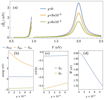
Figure 1: Anharmonic polariton energy distribution. (a) Stationary anharmonic polariton energy $\langle\hat{H}_{S}\rangle$ as a function of coupling strength $V$ for three different values in the anharmonicity constant $\chi$, $0$ (blue), $3\times 10^{-5}$ (orange), $6\times 10^{-5}$ (green). (b) Stationary exciton, phonon and interaction energy $E_{\rm TLS}$, $E_{\rm pho}$ and $E_{\rm int}$ (b) heat rates $\dot{Q}_{X}$ and $\dot{Q}_{P}$, and (d) total work $\overline{W}$ at resonance $V=2\omega$ as a function of the anharmonicity parameter $\chi$. Parameters for this system are $\omega^{\prime}=\omega=1.0$ eV, $\Gamma_{X}=0.2$ eV, $\Gamma_{P}=0.4$ eV, $A_{X}=0.1$ eV, $A_{P}=0$, $\varepsilon_{1}=0$, $\varepsilon_{2}=1.0$ eV, $T=300$ K. Propagation time $t=8.27$ ps.

The polariton thermodynamic properties in stationary state follow from its density matrix and the definitions for heat and work[43],

$$\dot{Q}_{\square}(t)= -{\rm Tr}\left[L_{\square}(t)\hat{H}_{\rm S}\right]$$ (10)

$$\dot{W}_{\square}(t)= -{\rm Tr}\left[L_{d\square}(t)\hat{H}_{\rm S}\right].\hskip 14.22636pt(\square=X,P),$$ (11)

where

$$L^{\;\;\beta_{1}}_{\square\,\alpha_{1}}=\sum_{\alpha_{2}\beta_{2}}\mathcal{L}^{\;\;\;\alpha_{1}\beta_{1}}_{\square\,\alpha_{2}\beta_{2}}\rho^{\beta_{2}}_{\alpha_{2}}(t)\hskip 14.22636pt(\square=X,P,dX,dP),$$ (12)

From the polariton’s von Neumann entropy

$$S(t)= -{\rm Tr}\left[\rho(t)\ln\rho(t)\right],$$ (13)

we obtain the entropy change rate

$$\dot{S}(t)= \sum_{\square=X,P}\dot{S}_{\square}(t)+\dot{S}_{d\square}(t),$$ (14)

$$\dot{S}_{\square}= {\rm Tr}\left[L_{\square}(t)\ln\rho(t)\right]\hskip 14.22636pt(\square=X,P,dX,dP),$$ (15)

which as a consequence of Spohn’s theorem[74, 75] provides the definition of irreversible heat rate relative to the polaritons equilibrium density matrix $\rho_{o}=e^{-\beta_{o}\hat{H}_{\rm S}}/{\rm Tr}[e^{-\beta_{o}\hat{H}_{\rm S}}]$, with $\beta_{o}=1/(k_{B}T_{\rm env})$ and $T_{\rm env}$ the absolute temperature

$$\dot{Q}_{\rm irrev}(t)= \beta_{o}^{-1}Tr[{(\mathcal{L}_{X}(t)+\mathcal{L}_{P}(t))(\ln\rho_{o}-\ln\rho(t)\,)]}$$

$$= \beta_{o}^{-1}(\dot{S}_{X}(t)+\dot{S}_{p}(t))-(\dot{Q}_{X}(t)+\dot{Q}_{P}(t)).$$ (16)

III Anharmonic polaritons

Next, we numerically investigate the polariton energy distribution between the exciton, phonon and interaction parts and how such distribution depends on the polariton’s anharmonic character and exciton-phonon coupling strength. We also analyze how energy dissipation depends on these factors. For simplicity, we consider the case where the driving field directly modulates the exciton by setting $A_{P}=0$ postponing until the next section the study of arbitrary external periodic drivings.

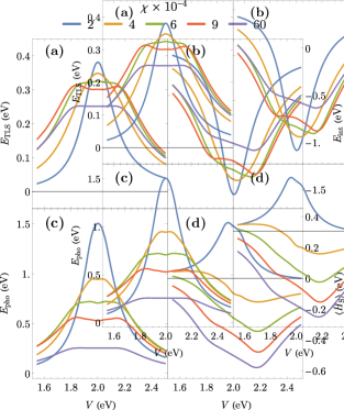
Figure 2: Energy distribution in strongly anharmonic polaritons. (a) Exciton energy $E_{\rm TLS}$ (b) exciton-phonon interaction energy $E_{\rm int}$, (c) phonon energy $E_{\rm pho}$, and (d) total energy $\langle\hat{H}_{\rm S}\rangle$ as a function of the exciton-phonon coupling strength $V$. The lineshapes shown are for polaritons with anharmonicity constant $\chi$ varying from $2\times 10^{-4}$ to $6\times 10^{-3}$. Other paremeters are as in Fig. 1.

We begin by studying the hybrid exciton-phonon total energy profile, as a function of the coupling strength $V$, and its deviation from the harmonic limit. Figure 1(a) shows $\langle\hat{H}_{S}\rangle$ for three polaritons characterized by different values in the anharmonicity constant $\chi$. The system with $\chi=0$ is the harmonic model analyzed in Ref. 43 when $\chi=0$. We note that while the qualitative dependence of the system energy $\langle H_{S}\rangle$ on $V$ is preserved in weakly anharmonic polaritons with $\chi<10^{-4}$, the total energy is consistently lower as the anharmonic character increases. Indeed, as illustrated in Fig. 1(b) for a polariton in resonance $V=2\omega$, the phonon energy $E_{\rm pho}$ for a system with $\chi=9\times 10^{-5}$ is about 50% of its expected value in the harmonic limit $\chi=0$, while the stationary $E_{\rm int}$ and $E_{\rm TLS}$ do not vary significantly. Thus, the observed energy difference is the result of the lower energy storage capacity in the phonon modes. Figure 1(c) shows the reversible heat rates reveling a linear decrease in the absolute value of both $\dot{Q}_{P}$ and $\dot{Q}_{X}$ with $\chi$. Similarly, the mean work rate in stationary state $\overline{W}$ decreases with an approximate linear dependence on $\chi$, as illustrated in Fig. 1(d), suggesting that even in the situation in which the driving field couples exclusively with the exciton, the phonon anharmonicity can modify the maximum power during periodic modulation.

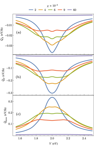
Figure 3: Reversible and irreversible heat rates in a periodically-driven strongly-anharmonic polariton. (a) $\dot{Q}_{X}$ (b)$\dot{Q}_{P}$ (c) $\dot{Q}_{\rm irrev}$ . The lineshapes shown are for polaritons with anharmonicity constant $\chi$ varying from $2\times 10^{-4}$ to $6\times 10^{-3}$. Other parameters are as in Fig. 1.

The functional dependence of the polariton energy on $V$ takes a remarkably different form from the one observed near the harmonic limit when the polariton’s anharmonicity character is stronger. For the particular system under consideration, we observe such transition in Fig. 2 occurring when $\chi>10^{-4}$. In constrast to the finding for weakly anharmonic systems, for $\chi$ between $10^{-4}$ and $10^{-3}$, we observe in Figs. 2(a) and 2(b) a decrease on the absolute exciton $E_{\rm TLS}$ and the interaction $E_{\rm int}$ energies near resonance. Moreover, the lineshape broadens for larger values in $\chi$, deviating from the Lorentzian form identified for the harmonic limit in Ref. [43], resulting incidentally in larger absolute exciton and interaction energies off-resonance. Significantly, the resonance energy varies from a highly excited state, close to the population inversion in the harmonic limit to one third population ratio. For an exciton decoupled to the phonon mode and under similar driving conditions, the weak damping rate allows for the exciton energy to reach values close to 0.5 eV corresponding to an excited population of $\rho_{2}\sim 0.5$, near saturation. We conclude that anharmonicity character is detrimental near resonance but can enhance the energy absorption at the exciton off-resonance (i.e., $V\neq 2\omega$). The phonon energy, presented in Fig. 2(c), follows a similar trend to the one observed for the exciton with a more considerable reduction in maximum energy with $\chi$. Consequently, we find in Fig. 2(d) that the total polariton energy is dominated by the interaction energy, leading to negative energy relative to the free exction ground state with a minimum in energy occurring off-resonance $V>2\omega$.

The functional dependence of reversible and irreversible heat rates on $V$ also changes with the polariton anharmonic character as illustrated in Fig. 3. The trends are similar to the ones described above for the phonon or exciton energies: broadening of the lineshape near resonance with the consequent decay the the absolute value of these rates at $V=2\omega$ with a relative increase off resonance. Remarkably, for $\chi>10^{-3}$, $E_{\rm pho}$, $\dot{Q}_{X}$, $\dot{Q}_{P}$ and $\dot{Q}_{\rm irrev}$ drop several orders of magnitude.

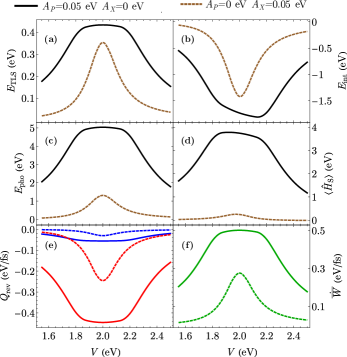
Figure 4: Contrasts in the energy distribution, dissipated heat and mean work performed on a periodically driven polariton when the external field couples to the exciton ($A_{X}=0.05$ eV and $A_{P}=0$, dashed lines) versus coupling to the phonon($A_{X}=0$ and $A_{P}=0.05$ eV, solid lines). (a) exciton energy $E_{\rm TLS}$ (b) interaction energy $E_{\rm int}$ (c) phonon energy $E_{\rm pho}$ (d) total energy $\langle\hat{H}_{\rm S}\rangle$, (e) reversible heat rates $\dot{Q}_{X}$ (blue), and $\dot{Q}_{P}$ (red), and (f) mean work rate $\dot{\overline{W}}$ . The polariton is harmonic with $\chi=0$. Other parameters are as in Fig. 1 .

IV External Driving protocols

In this section we study general driving regimes that include direct coupling of the external driving field to the phonon, which are expected to be relevant in, for instance, plasmonic cavities.

We begin by comparing the two extreme cases in which the driving field modulates exclusively the exciton and the phonon forming the harmonic polariton ($\chi=0$) in Fig. 4, where we juxtapose the stationary state for a periodically driven polariton in both cases. We take as the external driving coupling strengths $A_{X}=0.05$ eV and $A_{P}=0$ in one case, and $A_{X}=0$ and $A_{P}=0.05$ eV in the other one. All other parameters are identical, such that any observed dissimilarity results from differences in the driving protocols. In Fig. 4(a) we find that $E_{\rm TLS}$ is consistently smaller when the driving field modulates exclusively the exciton population for all values in $V$. Moreover, when the external field modulates the phonon, the exciton energy is nearly the saturation energy for an interval of $V$ values close to the resonance coupling strength $V=2\omega$, displaying a plateau in energy. Put it other way, this observation indicates that the exciton excited population is closed to the maximum allowed by the weak system interaction with the heat reservoir, suggesting also the lack of population inversion ($E_{TLS}<0.5$ such that $\rho_{2}<\rho_{1}$). The exciton-phonon coupling energy is also larger in absolute value when the external field couples to the phonon (see Fig. 4(b)). The phonon energy in Fig. 4(c) is also larger in this case, showing a plateau near resonance similar in form to the one observed for $E_{\rm TLS}$. Surprisingly, this finding reveals that $E_{\rm pho}$ can be limited by the maximum excited population achievable by the exciton when the exciton and phonon interact strongly. The total polariton energy, 4(d), is one order of magnitude larger when the field couples to the phonon only, and shows an asymmetry near resonance resulting from the linear dependence on $V$ of $E_{\rm int}$. We conclude that energy storage in the polariton is enhanced when the external field couples to the phonon in all cases. Figure 4(e) shows $\dot{Q}_{X}$ and $\dot{Q}_{P}$ revealing that these rates follow similar trends to those observed for $E_{\rm TLS}$ and $E_{\rm pho}$, as described above. Lastly, we find in Fig. 4(f) that the periodic driving of the phonon results in larger mean power $\dot{\overline{W}}$.

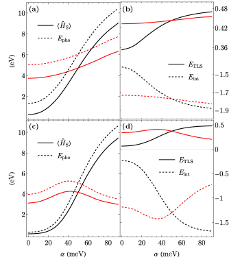
Figure 5: Simultaneous exciton and phonon driving. The black lines are for a protocol with fixed $A_{X}=0.05$ eV and varying $A_{P}$, such that $A_{P}=\alpha$. The read lines show the opposite situation, with $A_{X}=\alpha$ and fixed $A_{P}=0.05$. Panels (a) and (b) show energies in resonance, i.e., $V=2\omega$, while (c) and (d) are off resonance with $V=1.75\,\omega$. Panels (a) and (c) show total and phonon energy, $\langle\hat{H}_{\rm TLS}\rangle$ and $E_{\rm pho}$; (b) and (d) show the exciton and interaction energies, $E_{\rm TLS}$ and $E_{\rm pho}$, for each protocol. The polariton is harmonic with $\chi=0$ in all cases. Other parameters are as in Fig. 1.

Next, we analyze mixed situations in Fig. 5, where the external driving field couples simultaneously to both the exciton and the phonon with varying strengths $A_{X}$, $A_{P}$. Specifically, we consider how the total energy and its distribution changes when we fix either $A_{X}$ or $A_{P}$ to $0.05$ eV while modulating the other coupling parameter from $0$ to $0.09$ eV. Figures 5(a) and (b) present results for a polariton in resonance ($V=2\omega$). In this case, the total energy stored by the polariton is considerably enhanced by several orders of magnitude when $A_{P}$ increases in the range considered while we fixed $A_{X}$. In contrast, the inverted situation leads to an increase of nearly 50% and minor variations in $E_{\rm TLS}$ and $E_{\rm int}$. These patterns may change off-resonance. As an illustration, in Figs. 5(c) and (d) we investigate the same protocols when $V=1.75\omega$, finding a nonmonotonic change for fixed $A_{P}$ and varying $A_{X}$. Looking at the variation in $E_{\rm TLS}$, $E_{\rm pho}$, and $\langle\hat{H}_{\rm S}\rangle$, we observe that each one of these energies reaches its maximum value near $A_{X}=\alpha=0.04$ eV, resulting in a drop in the same as $A_{X}$ increases for $A_{X}>0.04$ eV. This observation suggests the occurrence of destructive interference between the exciton and photon dynamics induced by the external field for particular coupling strenghts during their simultaneous periodic driving.

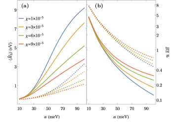
Figure 6: Total stored energy $\langle\hat{H}_{\rm S}\rangle$ (a) and driving efficiency %Eff Eq. (17) (b) for the periodic modulation of several anharmonic polaritons as a function of driving strengths $A_{X}$ and $A_{P}$. We show results for two driving forms: fixed $A_{X}=0$ and varying $A_{P}=\alpha$ (Solid lines), and varying $A_{X}=\alpha$ with fix $A_{P}=0$ (dashed lines). Other parameters are as in Fig. 1.

Finally, we return to our investigation of anharmonic polaritons in Fig. 6, where we show stationary state properties for several anharmonic polariton periodically modulated according to the two protocols discussed in Fig. 4. In this case we limit our consideration to polaritons in resonance, and find that for both protocols the total energy $\langle\hat{H}_{\rm S}\rangle$ decreases with $\chi$, and increases as the coupling term $A_{X}$ or $A_{P}$ (Fig. 6(a)). Moreover, the trend identified above, indicating that the energy stored in the polariton is larger when the external field modulates the phonon population persists in weakly anharmonic polaritons. Remarkably, considering the following figure of merit to evaluate the efficiency driving protocols

$${\rm Eff}=\frac{\bar{W}-\bar{Q}_{\rm irr}}{\bar{W}},$$ (17)

where $\bar{W}$ and $\bar{Q}_{\rm irr}$ are the mean work and irreversible heat per period, we observe in Fig. 6(b) higher efficiencies the larger $\chi$ is, in both protocols. The figure of merit in Eq. (17) is the ratio between the total energy transferred from the external field to the polariton and the actual “useful” energy in stationary state. In addition, the figure of merit in Eq. (17) quickly decays with the external field coupling strength. Surprisingly, the periodic modulation of the exciton population has consistently larger values in the figure of merit than the protocol driving the phonon. Based on these results, we conclude that while an external periodic field coupled to phonon favors larger energy storage in the polariton, the ratio between input energy and useful energy per period of time is smaller when compared with the direct modulation of exciton population.

V Conclusions

We presented a systematic study of the dynamics and thermodynamic properties of anharmonic polaritons under several periodic driving protocols. When the phonon in the polariton is weakly anharmonic, the energy distribution and thermodynamic properties are very similar to those observed in harmonic polaritons[43]. Still, when the anharmonic character is moderate or significant, the total stationary energy of the hybrid system is lower than the expected energy for the individual components. When the polariton is off-resonance, we observed destructive interference during the simultaneous exciton and phonon driving, resulting in lower exciton and phonon energies than those observed for the uncoupled components. Moreover, after defining a figure of merit for the polariton periodic modulation in terms of the ratio between the mean work and useful energy, we found that while an external periodic field coupled to the phonon enhances the polariton’s energy storage capacity, the ratio input energy useful energy per period is smaller than when the external field modulates only exciton population.

Appendix A Polariton energy distribution with weakly damped phonons

Figure 7: Energy distribution in a periodically-driven strongly-anharmonic polariton as a fxunction of the exciton-phonon coupling energy $V$, and for three different phonon relaxation rates $\Gamma_{P}=0.01$ (blue), $0.08$ (orange), and 0.4 (green) eV. (a) exciton energy $E_{\rm TLS}$ (b) interaction energy $E_{\rm int}$ (c) phonon energy $E_{\rm pho}$ and(d) total energy $\langle\hat{H}_{\rm S}\rangle$. Other parameters are as in Fig. 1.

Appendix B Propagator

In this section we demonstrate that under weak periodic driving, the propagation of an intial state is well described by the local-in-time propagator in Eq. (9)

Fist, we note that the QME in Eq. (8), can be written in the following form

$$\frac{d}{dt}\vec{\rho}(t)=-\left\{\mathcal{A}_{o}+f_{+}(t)\mathcal{A}_{+}+f_{-}(t)\mathcal{A}_{-}\right\}\vec{\rho(t)},$$ (18)

where $\mathcal{A}_{o}$ and $\mathcal{A}_{\pm}$ are time-independent matrices, and $f_{\pm}(t)=2\cos(\omega t)e^{\pm i\omega t}$. By direct integration we find

$$\vec{\rho}(t)=\vec{\rho}(0)-\int_{0}^{t}dt_{1}\left\{\mathcal{A}_{o}+f_{+}(t_{1})\mathcal{A}_{+}+f_{-}(t_{1})\mathcal{A}_{-}\right\}\vec{\rho}(t_{1})$$ (19)

and by sequential substitution we obtain the series

$$s_{o}= \vec{\rho}(0)$$ (20)

$$s_{n}(t)= s_{0}-\int_{0}^{t}dt_{n}\left\{\mathcal{A}_{o}+f_{+}(t_{n})\mathcal{A}_{+}+f_{-}(t_{n})\mathcal{A}_{-}\right\}s_{n-1}(t_{n}),$$ (21)

which leads to the solution to the differential equation Eq. (18) of the form

$$\vec{\rho}(t)=\sum_{n=0}^{\infty}(-1)^{n}I_{n}(t)\vec{\rho}(0),$$ (22)

with

$$I_{0}(t)= 1$$ (23)

$$I_{n}(t)= \int_{0}^{t}dt_{1}\left\{\mathcal{A}_{o}+f_{+}(t_{1})\mathcal{A}_{+}+f_{-}(t_{1})\mathcal{A}_{-}\right\}I_{n-1}(t_{1}).$$ (24)

Alternatively, we write

$$I_{n}(t)= \int_{0}^{t}dt_{1}\int_{0}^{t_{1}}dt_{2}\dots\int_{0}^{t_{n-1}}dt_{n}$$

$$\hskip 8.5359pt\prod_{k=1}^{n}\left\{\mathcal{A}_{o}+f_{+}(t_{k})\mathcal{A}_{+}+f_{-}(t_{k})\mathcal{A}_{-}\right\}$$ (25)

$$= \sum_{l\in 3^{n}}\left(\prod_{k=1}^{n}\mathcal{A}_{o}^{\delta_{0}^{l_{k}}}\mathcal{A}_{-}^{\delta_{-}^{l_{k}}}\mathcal{A}_{+}^{\delta_{+}^{l_{k}}}\right)\times$$

$$\hskip 19.91684pt\int_{0}^{t}dt_{1}f_{+}(t_{1})^{\delta_{+}^{l_{1}}}f_{-}(t_{1})^{\delta_{-}^{l_{1}}}$$

$$\hskip 39.83368pt\dots\int_{0}^{t_{n}-1}dt_{1}f_{+}(t_{n})^{\delta_{+}^{l_{n}}}f_{-}(t_{n})^{\delta_{-}^{l_{n}}}$$ (26)

Each $l\in 3^{n}$ is an $n$-tuple ${l_{1},\dots,l_{n}}$ with $\l_{i}=1,2,3$. Defining the correspondence $1\iff 0$, $1\iff-$, $3\iff+$; every $l$ corresponds to one term in the expansion of the product in Eq. (B).

We define

$$F(t,l_{i})=\int_{0}^{t}dt^{\prime}f_{+}(t^{\prime})^{\delta_{+}^{l_{i}}}f_{-}(t^{\prime})^{\delta_{-}^{l_{i}}},$$ (27)

such that

$$\frac{d}{dt}F(t,l_{i})=f_{+}(t)^{\delta_{+}^{l_{i}}}f_{-}(t)^{\delta_{-}^{l_{i}}}$$ (28)

and

$$I_{n}(t)= \sum_{l\in 3^{n}}\left(\prod_{k=1}^{n}\mathcal{A}_{o}^{\delta_{0}^{l_{k}}}\mathcal{A}_{-}^{\delta_{-}^{l_{k}}}\mathcal{A}_{+}^{\delta_{+}^{l_{k}}}\right)\times$$

$$\hskip 8.5359pt\int_{0}^{t}dt_{1}\frac{d}{dt_{1}}F(t_{1},l_{1})\dots\int_{0}^{t_{n}-1}dt_{1}\frac{d}{dt_{n}}F(t_{n},l_{n}).$$ (29)

Then we use integration by part to evaluate the integrals in Eq. (29) and the identity

$$\frac{t_{1}^{n-1}}{(n-1)!}=\int_{0}^{t_{1}}dt_{2}\dots\int_{0}^{t_{n-1}}dt_{n}.$$ (30)

As a result, we obtain the relation

$$\int_{0}^{t}dt_{1}\frac{d}{dt} F(t_{1},l_{1})\int_{0}^{t_{1}}dt_{2}\dots\int_{0}^{t_{n-1}}dt_{n}=$$

$$F(t,l_{1})\frac{t_{1}^{n-1}}{(n-1)!}-\int_{0}^{t}dt_{1}F(t_{1},l_{1})\frac{t_{1}^{n-1}}{(n-1)!},$$ (31)

from which we collect the first term and obtain the exponential form for the propagator. The excluded terms in this expansion are bounded by the field amplitude. In addition, this result shows that the sequence is uniformly convergent and the the propagator time-local.

References

- Li et al. [2021] T. E. Li, B. Cui, J. E. Subotnik, and A. Nitzan, Molecular polaritonics: Chemical dynamics under strong light–matter coupling, Annual review of physical chemistry 73 (2021).
- Dunkelberger et al. [2022] A. D. Dunkelberger, B. S. Simpkins, I. Vurgaftman, and J. C. Owrutsky, Vibration-cavity polariton chemistry and dynamics, Annual Review of Physical Chemistry 73 (2022).
- Fofang et al. [2011] N. T. Fofang, N. K. Grady, Z. Fan, A. O. Govorov, and N. J. Halas, Plexciton dynamics: exciton- plasmon coupling in a j-aggregate- au nanoshell complex provides a mechanism for nonlinearity, Nano letters 11, 1556 (2011).
- Bitton and Haran [2022] O. Bitton and G. Haran, Plasmonic cavities and individual quantum emitters in the strong coupling limit, Accounts of chemical research 55, 1659 (2022).
- Mondal et al. [2022] M. Mondal, M. A. Ochoa, M. Sukharev, and A. Nitzan, Coupling, lifetimes, and “strong coupling” maps for single molecules at plasmonic interfaces, The Journal of Chemical Physics 156, 154303 (2022).
- [6] M. Mondal, A. Semenov, M. A. Ochoa, and A. Nitzan, Strong coupling in infrared plasmonic cavities, The Journal of Physical Chemistry Letters 13, 9673.
- Kaitouni et al. [2006] R. I. Kaitouni, O. El Daïf, A. Baas, M. Richard, T. Paraiso, P. Lugan, T. Guillet, F. Morier-Genoud, J. Ganière, J. Staehli, et al., Engineering the spatial confinement of exciton polaritons in semiconductors, Physical Review B 74, 155311 (2006).
- Deng et al. [2010] H. Deng, H. Haug, and Y. Yamamoto, Exciton-polariton bose-einstein condensation, Reviews of modern physics 82, 1489 (2010).
- Byrnes et al. [2014] T. Byrnes, N. Y. Kim, and Y. Yamamoto, Exciton–polariton condensates, Nature Physics 10, 803 (2014).
- Ochoa et al. [2020] M. A. Ochoa, J. E. Maslar, and H. S. Bennett, Extracting electron densities in n-type gaas from raman spectra: Comparisons with hall measurements, Journal of applied physics 128, 075703 (2020).
- Khan et al. [2021] W. Khan, P. P. Potts, S. Lehmann, C. Thelander, K. A. Dick, P. Samuelsson, and V. F. Maisi, Efficient and continuous microwave photoconversion in hybrid cavity-semiconductor nanowire double quantum dot diodes, Nature communications 12, 1 (2021).
- Denning et al. [2022] E. V. Denning, M. Wubs, N. Stenger, J. Mørk, and P. T. Kristensen, Cavity-induced exciton localization and polariton blockade in two-dimensional semiconductors coupled to an electromagnetic resonator, Physical Review Research 4, L012020 (2022).
- Pigeau et al. [2015] B. Pigeau, S. Rohr, L. Mercier de Lépinay, A. Gloppe, V. Jacques, and O. Arcizet, Observation of a phononic mollow triplet in a multimode hybrid spin-nanomechanical system, Nature Communications 6, 1 (2015).
- Li et al. [2016] P.-B. Li, Z.-L. Xiang, P. Rabl, and F. Nori, Hybrid quantum device with nitrogen-vacancy centers in diamond coupled to carbon nanotubes, Physical review letters 117, 015502 (2016).
- Muñoz et al. [2018] C. S. Muñoz, A. Lara, J. Puebla, and F. Nori, Hybrid systems for the generation of nonclassical mechanical states via quadratic interactions, Physical review letters 121, 123604 (2018).
- Blais et al. [2021] A. Blais, A. L. Grimsmo, S. M. Girvin, and A. Wallraff, Circuit quantum electrodynamics, Reviews of Modern Physics 93, 025005 (2021).
- Kurizki et al. [2015] G. Kurizki, P. Bertet, Y. Kubo, K. Mølmer, D. Petrosyan, P. Rabl, and J. Schmiedmayer, Quantum technologies with hybrid systems, Proceedings of the National Academy of Sciences 112, 3866 (2015).
- Ghosh and Liew [2020] S. Ghosh and T. C. Liew, Quantum computing with exciton-polariton condensates, npj Quantum Information 6, 16 (2020).
- Guan et al. [2022] J. Guan, J.-E. Park, S. Deng, M. J. Tan, J. Hu, and T. W. Odom, Light–matter interactions in hybrid material metasurfaces, Chemical Reviews 122, 15177 (2022).
- Li et al. [2022a] T. E. Li, B. Cui, J. E. Subotnik, and A. Nitzan, Molecular polaritonics: Chemical dynamics under strong light–matter coupling, Annual review of physical chemistry 73, 43 (2022a).
- Mandal et al. [2023] A. Mandal, M. A. Taylor, B. M. Weight, E. R. Koessler, X. Li, and P. Huo, Theoretical advances in polariton chemistry and molecular cavity quantum electrodynamics, Chemical Reviews 123, 9786 (2023).
- Campos-Gonzalez-Angulo et al. [2023] J. Campos-Gonzalez-Angulo, Y. Poh, M. Du, and J. Yuen-Zhou, Swinging between shine and shadow: Theoretical advances on thermally activated vibropolaritonic chemistry, The Journal of Chemical Physics 158 (2023).
- Shore and Knight [1993] B. W. Shore and P. L. Knight, The jaynes-cummings model, Journal of Modern Optics 40, 1195 (1993).
- Casanova et al. [2010] J. Casanova, G. Romero, I. Lizuain, J. J. García-Ripoll, and E. Solano, Deep strong coupling regime of the jaynes-cummings model, Physical review letters 105, 263603 (2010).
- Bina [2012] M. Bina, The coherent interaction between matter and radiation: A tutorial on the jaynes-cummings model, The European Physical Journal Special Topics 203, 163 (2012).
- Larson and Mavrogordatos [2022] J. Larson and T. K. Mavrogordatos, The jaynes-cummings model and its descendants, arXiv preprint arXiv:2202.00330 (2022).
- Fink et al. [2009] J. Fink, R. Bianchetti, M. Baur, M. Göppl, L. Steffen, S. Filipp, P. J. Leek, A. Blais, and A. Wallraff, Dressed collective qubit states and the tavis-cummings model in circuit qed, Physical review letters 103, 083601 (2009).
- Agarwal et al. [2012] S. Agarwal, S. H. Rafsanjani, and J. Eberly, Tavis-cummings model beyond the rotating wave approximation: Quasidegenerate qubits, Physical Review A 85, 043815 (2012).
- Zhu et al. [2016] C. Zhu, L. Dong, and H. Pu, Effects of spin-orbit coupling on jaynes-cummings and tavis-cummings models, Physical Review A 94, 053621 (2016).
- Sun et al. [2022] K. Sun, C. Dou, M. F. Gelin, and Y. Zhao, Dynamics of disordered tavis–cummings and holstein–tavis–cummings models, The Journal of Chemical Physics 156 (2022).
- Campos-Gonzalez-Angulo et al. [2021] J. A. Campos-Gonzalez-Angulo, R. F. Ribeiro, and J. Yuen-Zhou, Generalization of the tavis–cummings model for multi-level anharmonic systems, New Journal of Physics 23, 063081 (2021).
- Xie et al. [2017] Q. Xie, H. Zhong, M. T. Batchelor, and C. Lee, The quantum rabi model: solution and dynamics, Journal of Physics A: Mathematical and Theoretical 50, 113001 (2017).
- Rossatto et al. [2017] D. Z. Rossatto, C. J. Villas-Bôas, M. Sanz, and E. Solano, Spectral classification of coupling regimes in the quantum rabi model, Physical Review A 96, 013849 (2017).
- Chen et al. [2008] Q.-H. Chen, Y.-Y. Zhang, T. Liu, and K.-L. Wang, Numerically exact solution to the finite-size dicke model, Physical Review A 78, 051801 (2008).
- Garraway [2011] B. M. Garraway, The dicke model in quantum optics: Dicke model revisited, Philosophical Transactions of the Royal Society A: Mathematical, Physical and Engineering Sciences 369, 1137 (2011).
- Garraway [1997] B. Garraway, Nonperturbative decay of an atomic system in a cavity, Physical Review A 55, 2290 (1997).
- Wang et al. [2021] D. S. Wang, T. Neuman, J. Flick, and P. Narang, Light–matter interaction of a molecule in a dissipative cavity from first principles, The Journal of Chemical Physics 154 (2021).
- Deffner [2014] S. Deffner, Optimal control of a qubit in an optical cavity, Journal of Physics B: Atomic, Molecular and Optical Physics 47, 145502 (2014).
- Li et al. [2022b] T. E. Li, A. Nitzan, and J. E. Subotnik, Polariton relaxation under vibrational strong coupling: Comparing cavity molecular dynamics simulations against fermi’s golden rule rate, The Journal of Chemical Physics 156 (2022b).
- Barnett and Knight [1986] S. Barnett and P. Knight, Dissipation in a fundamental model of quantum optical resonance, Physical Review A 33, 2444 (1986).
- del Pino et al. [2015] J. del Pino, J. Feist, and F. J. Garcia-Vidal, Quantum theory of collective strong coupling of molecular vibrations with a microcavity mode, New Journal of Physics 17, 053040 (2015).
- Martínez-Martínez and Yuen-Zhou [2018] L. A. Martínez-Martínez and J. Yuen-Zhou, Comment on ‘quantum theory of collective strong coupling of molecular vibrations with a microcavity mode’, New Journal of Physics 20, 018002 (2018).
- Ochoa [2022] M. A. Ochoa, Quantum thermodynamics of periodically driven polaritonic systems, Physical Review E 106, 064113 (2022).
- Bleu et al. [2023] O. Bleu, K. Choo, J. Levinsen, and M. M. Parish, Effective dissipative light-matter coupling in nonideal cavities, arXiv preprint arXiv:2301.02221 (2023).
- Bamba and Ogawa [2012] M. Bamba and T. Ogawa, Dissipation and detection of polaritons in the ultrastrong-coupling regime, Physical Review A 86, 063831 (2012).
- Sieberer et al. [2013] L. Sieberer, S. D. Huber, E. Altman, and S. Diehl, Dynamical critical phenomena in driven-dissipative systems, Physical review letters 110, 195301 (2013).
- Drezet [2017] A. Drezet, Quantizing polaritons in inhomogeneous dissipative systems, Physical Review A 95, 023831 (2017).
- Pistorius et al. [2020] T. Pistorius, J. Kazemi, and H. Weimer, Quantum many-body dynamics of driven-dissipative rydberg polaritons, Physical Review Letters 125, 263604 (2020).
- Kyriienko et al. [2014] O. Kyriienko, T. C. H. Liew, and I. A. Shelykh, Optomechanics with cavity polaritons: dissipative coupling and unconventional bistability, Physical review letters 112, 076402 (2014).
- Liu et al. [2014] Y.-C. Liu, X. Luan, H.-K. Li, Q. Gong, C. W. Wong, and Y.-F. Xiao, Coherent polariton dynamics in coupled highly dissipative cavities, Physical Review Letters 112, 213602 (2014).
- Pekola [2015] J. P. Pekola, Towards quantum thermodynamics in electronic circuits, Nature Physics 11, 118 (2015).
- Esposito et al. [2015a] M. Esposito, M. A. Ochoa, and M. Galperin, Quantum thermodynamics: A nonequilibrium green’s function approach, Physical review letters 114, 080602 (2015a).
- Vinjanampathy and Anders [2016] S. Vinjanampathy and J. Anders, Quantum thermodynamics, Contemporary Physics 57, 545 (2016).
- Deffner and Campbell [2019] S. Deffner and S. Campbell, Quantum Thermodynamics: An introduction to the thermodynamics of quantum information (Morgan & Claypool Publishers, 2019).
- Kosloff [2019] R. Kosloff, Quantum thermodynamics and open-systems modeling, The Journal of chemical physics 150, 204105 (2019).
- Kurizki and Kofman [2022] G. Kurizki and A. G. Kofman, Thermodynamics and Control of Open Quantum Systems (Cambridge University Press, 2022).
- Talkner et al. [2007] P. Talkner, E. Lutz, and P. Hänggi, Fluctuation theorems: Work is not an observable, Physical Review E 75, 050102 (2007).
- Esposito et al. [2015b] M. Esposito, M. A. Ochoa, and M. Galperin, Nature of heat in strongly coupled open quantum systems, Physical Review B 92, 235440 (2015b).
- Whitney et al. [2018] R. S. Whitney, R. Sánchez, and J. Splettstoesser, Quantum thermodynamics of nanoscale thermoelectrics and electronic devices, in Thermodynamics in the quantum regime (Springer, 2018) pp. 175–206.
- Kalaee and Wacker [2021] A. A. S. Kalaee and A. Wacker, Positivity of entropy production for the three-level maser, Physical Review A 103, 012202 (2021).
- Esposito et al. [2015c] M. Esposito, M. A. Ochoa, and M. Galperin, Efficiency fluctuations in quantum thermoelectric devices, Physical Review B 91, 115417 (2015c).
- Ochoa et al. [2015] M. A. Ochoa, Y. Selzer, U. Peskin, and M. Galperin, Pump–probe noise spectroscopy of molecular junctions, The journal of physical chemistry letters 6, 470 (2015).
- Chen et al. [2023] R. Chen, T. Gibson, and G. T. Craven, Energy transport between heat baths with oscillating temperatures, Physical Review E 108, 024148 (2023).
- Hotz and Schaller [2021] R. Hotz and G. Schaller, Coarse-graining master equation for periodically driven systems, Physical Review A 104, 052219 (2021).
- Tanimura [2020] Y. Tanimura, Numerically “exact” approach to open quantum dynamics: The hierarchical equations of motion (heom), The Journal of chemical physics 153, 020901 (2020).
- Wacker [2022] A. Wacker, Nonresonant two-level transitions: Insights from quantum thermodynamics, Physical Review A 105, 012214 (2022).
- Hone et al. [2009] D. W. Hone, R. Ketzmerick, and W. Kohn, Statistical mechanics of floquet systems: The pervasive problem of near degeneracies, Physical Review E 79, 051129 (2009).
- Restrepo et al. [2018] S. Restrepo, J. Cerrillo, P. Strasberg, and G. Schaller, From quantum heat engines to laser cooling: Floquet theory beyond the born–markov approximation, New Journal of Physics 20, 053063 (2018).
- Deng et al. [2016] C. Deng, F. Shen, S. Ashhab, and A. Lupascu, Dynamics of a two-level system under strong driving: Quantum-gate optimization based on floquet theory, Physical Review A 94, 032323 (2016).
- Wang and Dou [2023] Y. Wang and W. Dou, Nonadiabatic dynamics near metal surfaces under floquet engineering: Floquet electronic friction vs. floquet surface hopping, arXiv preprint arXiv:2306.06128 (2023).
- Bätge et al. [2023] J. Bätge, Y. Wang, A. Levy, W. Dou, and M. Thoss, Periodically driven open quantum systems with vibronic interaction: Resonance effects and vibrationally mediated decoupling, Physical Review B 108, 195412 (2023).
- [72] Y. Wang, V. Mosallanejad, W. Liu, and W. Dou, Nonadiabatic dynamics near metal surfaces with periodic drivings: A generalized surface hopping in floquet representation, Journal of Chemical Theory and Computation .
- Campos-Gonzalez-Angulo and Yuen-Zhou [2022] J. A. Campos-Gonzalez-Angulo and J. Yuen-Zhou, Generalization of the tavis–cummings model for multi-level anharmonic systems: Insights on the second excitation manifold, The Journal of Chemical Physics 156 (2022).
- Spohn [1978] H. Spohn, Entropy production for quantum dynamical semigroups, Journal of Mathematical Physics 19, 1227 (1978).
- Alicki [1979] R. Alicki, The quantum open system as a model of the heat engine, Journal of Physics A: Mathematical and General 12, L103 (1979).