Constructing Bayesian Optimal Designs for Discrete Choice Experiments by Simulated Annealing

Abstract

Discrete Choice Experiments (DCEs) investigate the attributes that influence individuals’ choices when selecting among various options. To enhance the quality of the estimated choice models, researchers opt for Bayesian optimal designs that utilize existing information about the attributes’ preferences. Given the nonlinear nature of choice models, the construction of an appropriate design requires efficient algorithms. Among these, the Coordinate-Exchange (CE) algorithm is most commonly employed for constructing designs based on the multinomial logit model. Since this is a hill-climbing algorithm, obtaining better designs necessitates multiple random starting designs. This approach increases the algorithm’s run-time, but may not lead to a significant improvement in results. We propose the use of a Simulated Annealing (SA) algorithm to construct Bayesian $\mathcal{D}$-optimal designs. This algorithm accepts both superior and inferior solutions, avoiding premature convergence and allowing a more thorough exploration of potential designs. Consequently, it ultimately obtains higher-quality choice designs within the same time-frame. Our work represents the first application of an SA algorithm in constructing Bayesian optimal designs for DCEs. Through computational experiments and a real-life case study, we demonstrate that the SA designs consistently outperform the CE designs in terms of Bayesian $\mathcal{D}$-efficiency, especially when the prior preference information is highly uncertain.

Keywords: Discrete Choice Experiments; Bayesian Optimal Design; Algorithm; Simulated Annealing; Coordinate Exchange

1 Introduction

Discrete Choice Experiments (DCEs) are frequently used to study consumer preferences for the attributes of various goods and have been widely used in fields such as marketing (Rossi and Allenby,, 2003; Train,, 2009), health care (Luyten et al.,, 2015), and transportation (Zijlstra et al.,, 2019). Typically, in a DCE, respondents are provided with a group of choice sets containing different alternatives or profiles that are defined by combinations of attribute levels associated with the product or service being studied. By observing and analyzing respondents’ selections within these choice sets, researchers can estimate the attractiveness of each attribute and level and further make predictions about consumers’ behaviors in real-world scenarios.

When planning DCEs, researchers often face the challenge of conducting experiments that can be costly, cumbersome, and time-consuming. The construction of Bayesian $\mathcal{D}$-optimal designs ensures that these experiments deliver accurate parameter estimations and precise predictions (Kessels et al.,, 2006). Given that choice models are nonlinear in their parameters, the Bayesian design methodology offers a robust solution for nonlinear choice design by incorporating a prior distribution into the formulation of the optimality criterion, thereby avoiding the necessity of specifying point parameter values (Sándor and Wedel,, 2001).

Since Bayesian optimal designs are difficult to construct theoretically, search algorithms are frequently employed to derive these designs, such as the the modified Federov algorithm (Cook and Nachtsheim,, 1980; Kessels et al.,, 2006), the Relabeling and Swapping (RS) algorithm (Huber and Zwerina,, 1996), the Relabeling, Swapping, and Cycling (RSC) algorithm (Sándor and Wedel,, 2001) and the Coordinate-Exchange (CE) algorithm (Meyer and Nachtsheim,, 1995; Kessels et al.,, 2009). In current DCEs, the CE algorithm is most widely used due to its relatively rapid execution speed. This algorithm can be viewed as a special case of a greedy profile-exchange algorithm. During its iterative process, the CE algorithm modifies only one “coordinate” or attribute level in a given profile, instead of exploring all possible combinations of attribute levels within the profile.

The CE algorithm begins with the generation of a random starting design and improves this design by evaluating changes on an attribute-by-attribute basis. For each attribute in each profile of the design, the value of the optimality criterion is calculated across all levels of that attribute. A level is only updated if the resulting new design yields a superior criterion value. This procedure is repeated until all profiles of the design are completed. If any attribute level changes in the current cycle, another complete cycle or iteration through the design is undertaken. This process is continued until no changes occur in a complete cycle or a predefined maximum number of iterations is reached. The candidate-set-free nature of the CE algorithm gives it a significant advantage, particularly in scenarios where profiles contain a large number of attributes or attribute levels (Kessels et al.,, 2009).

Because the CE algorithm is a heuristic optimization algorithm, it cannot guarantee that the resulting design is globally optimal. To increase the quality of the solution, a common practice is to initiate the algorithm with multiple random starting designs (Kessels et al.,, 2009; Goos and Jones,, 2011). However, given that these random starting points are independent of each other, adding a new starting point does not necessarily guarantee a better design. This results in a substantial amount of redundant computations, significantly increasing the algorithm’s run time. Consequently, this paper proposes the adoption of an algorithm that does not require multiple starting points, that is the Simulated Annealing (SA) algorithm, for obtaining superior Bayesian optimal choice designs within the same time frame.

The SA method was first proposed by Kirkpatrick et al., (1983) for finding the global minimum of a cost function that may possess several local minima. For a given objective function, the SA algorithm initiates from a random or specific starting point, coupled with a relatively high initial temperature. As the algorithm progresses, the temperature is gradually decreased until it reaches a predetermined termination criterion. At each temperature level, the algorithm generates a new solution by adding a random perturbation to the old solution and accepts this new solution based on specific rules. The probability of acceptance is calculated with reference to the annealing process in metallurgy, which is also the origin of the name “Simulated Annealing”. More specifically, if the new solution is superior to the current one, it is accepted. If not, the decision to accept the solution is made based on certain criteria, such as the Metropolis acceptance criterion (Metropolis et al.,, 1953). This approach allows for the acceptance of new solutions that may initially worsen the objective function value, particularly at higher temperatures. Such flexibility enables the algorithm to escape local optima. As the temperature is slowly lowered, the algorithm is more likely to converge to a global optimum.

The SA algorithm is widely employed in various optimization problems due to its efficiency in globally exploring for more possible solutions, such as in traveling salesman problems (Aarts et al.,, 1988; Malek et al.,, 1989) and knapsack problems (Liu et al.,, 2006; Qian and Ding,, 2007). However, its application in the field of optimal experimental design is relatively scarce. To the best of our knowledge, only a few studies, namely Bohachevsky et al., (1986), Meyer and Nachtsheim, (1988) and Angelis et al., (2001) have delved into this area. Nonetheless, these works primarily focus on optimal exact experimental designs based on Gaussian models. Their approaches have not been applied to choice models, nor Bayesian optimal designs for these models, thus differing significantly from our research. Our work is the inaugural application of the SA algorithm in constructing Bayesian optimal designs for DCEs. Through extensive computational experiments and a real-life application, we evaluate the performance of both the CE and SA algorithms, observing that the SA designs invariably surpass the CE designs, particularly when the prior preference information is highly uncertain.

The rest of the paper is organized as follows. In Section 2, we introduce the multinomial logit model and the Bayesian $\mathcal{D}$-optimal design approach. In Section 3, we describe how to apply the SA algorithm to construct Bayesian $\mathcal{D}$-optimal designs. In Section 4, we set up computational experiments to evaluate the performance of the SA algorithm against the CE algorithm. In Section 5, we apply our algorithms to a real-life case study. Finally, in Section 6, we discuss the results and future research directions.

2 The Multinomial Logit Model and Bayesian $\mathcal{D}$-optimality

We introduce the multinomial logit model with notations from Train, (2009), and explain how to construct Bayesian $\mathcal{D}$-optimal designs for this model.

2.1 Multinomial Logit Model

The multinomial logit model assumes that respondents to a DCE belong to a target group of decision makers with homogeneous preferences. The model employs random utility theory which describes the utility that a respondent attaches to profile $j$ ($j=1,\dots,J$) in choice set $s$ ($s=1,\dots,S$) as the sum of a systematic and a stochastic component:

$$U_{js}={\boldsymbol{x}}^{\prime}_{js}\boldsymbol{\beta}+\varepsilon_{js}.$$ (1)

In the systematic component ${\boldsymbol{x}}^{\prime}_{js}\boldsymbol{\beta}$, ${\boldsymbol{x}}_{js}$ is a $m\times 1$ vector containing the attribute levels of profile $j$ in choice set $s$. The vector $\boldsymbol{\beta}$ is a $m\times 1$ vector of parameter values representing the effects of the attribute levels on the utility. This parameter vector is the same for every respondent. The stochastic component $\varepsilon_{js}$ is the error term, which is assumed independently and identically extreme value distributed. Therefore, the multinomial logit probability that a respondent chooses profile $j$ in choice set $s$ is the closed-form expression

$$p_{js}=\frac{\mbox{exp}\left({\boldsymbol{x}}^{\prime}_{js}\boldsymbol{\beta}\right)}{\sum_{j=1}^{J}\mbox{exp}\left({\boldsymbol{x}}^{\prime}_{js}\boldsymbol{\beta}\right)},$$ (2)

where $\boldsymbol{\beta}$ can be estimated using a maximum likelihood approach.

2.2 Bayesian $\mathcal{D}$-optimal Design

The $\mathcal{D}$-optimality criterion has been most often employed to construct efficient choice designs (Huber and Zwerina,, 1996; Sándor and Wedel,, 2001). The $\mathcal{D}$-optimality criterion focuses on precise estimation of the parameters by maximizing the determinant of the information matrix related to the model under investigation. Given a design matrix $\bf{X}$ and parameter vector $\boldsymbol{\beta}$, the $\mathcal{D}$-optimality criterion can be defined as

$$\mathcal{D}=\mbox{log}\left|{\bf M}\left({\bf X},\boldsymbol{\beta}\right)\right|,$$ (3)

where ${\bf M}\left({\bf X},\boldsymbol{\beta}\right)$ is the information matrix of the parameter estimates. For the multinominal logit model, the information matrix ${\bf M}\left({\bf X},\boldsymbol{\beta}\right)$ can be obtained as the sum of the information matrices of each of the $S$ choice sets:

$${\bf M}\left({\bf X},\boldsymbol{\beta}\right)=\sum_{s=1}^{S}{\bf X}^{\prime}_{s}\left({\bf P}_{s}-{\bf p}_{s}{\bf p}^{\prime}_{s}\right){\bf X}_{s},$$ (4)

where $\bf{X}=(\bf{X}_{1},...,\bf{X}_{S})$ represents the model matrix over all choice sets, ${\bf P}_{s}=\mbox{diag}\left({\bf p}_{s}\right)$ with ${\bf p}_{s}=\left(p_{1s},\dots,p_{Js}\right)^{\prime}$ denoting the multinomial logit probabilities corresponding to all alternatives in choice set $s$.

Since the information matrix ${\bf M}\left({\bf X},\boldsymbol{\beta}\right)$ depends on the unknown parameter vector $\boldsymbol{\beta}$ through the choice probabilities, a prior distribution is often specified on the model parameters, which leads to the Bayesian optimal design (Kessels et al., 2011b, ; Ruseckaite et al.,, 2017). The Bayesian $\mathcal{D}$-optimality criterion seeks to maximize the determinant of the information matrix averaged over the prior distribution $\pi(\boldsymbol{\beta})$, and is defined as

$$\mathcal{D}_{B}=\int_{\mathcal{R}^{m}}\mbox{log}\left|{\bf M}\left({\bf X},\boldsymbol{\beta}\right)\right|\pi(\boldsymbol{\beta})\mbox{d}\boldsymbol{\beta}.$$ (5)

Since the formula in Eq. (5) has no closed-form solution, the Bayesian $\mathcal{D}$-optimality criterion is usually numerically approximated by taking draws from the prior distribution. In our work, we adopted the sampling methodology developed by Gotwalt et al., (2009), which is based on the radial-spherical integration rule initially proposed by Monahan and Genz, (1997). This method decomposes the integral in Eq. (5) into a radial and a spherical surface component. The radial integration leverages the generalized Gauss-Laguerre quadrature, while the spherical integration employs a randomly rotated extended simplex quadrature (Mysovskikh,, 1980). Yu et al., (2010) have demonstrated the superiority of quadrature methods over alternative approaches in assessing the Bayesian optimality criterion.

For the purpose of comparing the performance of two experimental designs with the same number of choice sets and profiles in each choice set, we adopt the relative $\mathcal{D}_{B}$-efficiency as a measure (Holling and Schwabe,, 2011). The Bayesian $\mathcal{D}$-efficiency of a design $\bf X$, relative to another design $\bf X^{*}$ can be defined as

$$\mathcal{D}_{B}\text{-eff}(\mathbf{X},\mathbf{X^{*}})=\exp\left(\frac{\mathcal{D}_{B}(\mathbf{X})-\mathcal{D}_{B}(\mathbf{X^{*}})}{\textit{m}}\right).$$ (6)

In terms of $\mathcal{D}_{B}\text{-eff}(\bf{X},\bf{X^{*}})$, a value of 1 indicates equivalent performance between the two designs. A value greater than 1 suggests that design $\bf X$ outperforms design $\bf X^{*}$. Conversely, a value less than 1 implies superior performance of design $\bf X^{*}$.

3 Simulated Annealing Algorithm

We describe how we apply the SA algorithm to construct Bayesian $\mathcal{D}$-optimal designs for DCEs. In Section 3.1, we provide a standard description of the SA algorithm for Bayesian design generation, and in Section 3.2, we delve into the details of the SA algorithm’s parameter settings.

3.1 Standard Description of the Simulated Annealing Algorithm

Input : Initial random choice design $\mathbf{X}$

Output : The best choice design $\mathbf{X}_{Best}$ found by the algorithm

1 Set a value for Initial Temperature $T_{0}$ by a random walk approach;

2 Set the number of iterations $k=0$;

3 Set $\mathbf{X}_{Best}=\mathbf{X}$;

4 while Stopping Criterion not met do

5       Update temperature $T_{k}$ according to a Cooling Function $f(k,T_{0})$ such that: $T_{k}=\frac{T_{0}}{k+1}$;

6       Define the new design $\mathbf{X^{\prime}}$ such that $\mathbf{X^{\prime}}$ is a transformation of $\mathbf{X}$ where one attribute in one profile is changed;

7       Let $\mathcal{D}_{B}(\mathbf{X})$ be the Bayesian $\mathcal{D}$-optimality criterion for the choice design $\mathbf{X}$. Accept $\mathbf{X^{\prime}}$ as the new solution with probability $\alpha$ such that:

$$\alpha(\mathbf{X},\mathbf{X^{\prime}})=\min\left\{1,\exp\left(\frac{\mathcal{D}_{B}(\mathbf{X^{\prime}})-\mathcal{D}_{B}(\mathbf{X})}{T_{k}}\right)\right\}$$ (7)

8       if $\mathbf{X^{\prime}}$ is accepted then

9             Set $\mathbf{X}=\mathbf{X^{\prime}}$;

10             if $\mathcal{D}_{B}(\mathbf{X})>\mathcal{D}_{B}(\mathbf{X}_{Best})$ then

11                   $\mathbf{X}_{Best}=\mathbf{X}$;

12                   $T_{Best}=T_{k}$;

13                  

14             end if

15            

16       end if

17      $k=k+1$;

18       if no new solutions are accepted in the last 1000 iterations then

19            Reset the temperature to a higher value $T_{New}$ according to a Reheating Scheme such that:

20             $T_{New}=2T_{Best}$;

21             $k=\frac{T_{0}}{T_{New}}-1$;

22            

23       end if

24      

25 end while

return $\mathbf{X}_{Best}$

Algorithm 1 Pseudo code for Simulated Annealing

The SA algorithm is defined in Algorithm 1. This algorithm starts by taking an initial random choice design $\mathbf{X}$ as input. It then proceeds to determine an appropriate value of the Initial Temperature $T_{0}$ by using a random walk approach. After that, the algorithm sets the number of iterations $k$ to $0$ and memorizes $\mathbf{X}$ as the current best choice design $\mathbf{X}_{Best}$. Starting from $T_{0}$, in each iteration, we employ a Cooling Function $f(k,T_{0})$ to update the current system temperature $T_{k}$. At the same time, we create a new choice design $\bf X^{\prime}$ by randomly selecting a profile from $\bf X$ and modifying one of the attributes (once again, randomly chosen). This results in a relatively minor perturbation to $\bf X$, facilitating exhaustive search by the algorithm. The new design $\bf X^{\prime}$ is assessed against the current design $\mathbf{X}$ by using the the Metropolis acceptance criterion as defined in Eq. (7). The main reason we use this criterion is that it will always lead to two cases:

If $\mathcal{D}_{B}(\mathbf{X^{\prime}})\geq\mathcal{D}_{B}(\mathbf{X})$:

Then we know that $e^{\frac{\mathcal{D}_{B}(\mathbf{X^{\prime}})-\mathcal{D}_{B}(\mathbf{X})}{T_{k}}}\geq 1$ and $\alpha=1$. We accept $\mathbf{X^{\prime}}$ every time, or probability $\alpha$ is 1.

If $\mathcal{D}_{B}(\mathbf{X^{\prime}})<\mathcal{D}_{B}(\mathbf{X})$:

Then we know that $e^{\frac{\mathcal{D}_{B}(\mathbf{X^{\prime}})-\mathcal{D}_{B}(\mathbf{X})}{T_{k}}}<1$ and $\alpha<1$. We accept $\mathbf{X^{\prime}}$ with probability $\alpha$. Note that the “worse” the value of $\mathcal{D}_{B}(\mathbf{X^{\prime}})$ compared to $\mathcal{D}_{B}(\mathbf{X})$, the smaller the value of $\alpha$.

When an accepted solution $\bf X^{\prime}$ also exhibits better performance than the best design so far, it is then adopted as the best design $\mathbf{X}_{Best}$, with the system temperature $T_{k}$ at that iteration being duly recorded as $T_{Best}$. In each iteration, $k$ is increased by $1$, leading to a corresponding decrease in $T_{k}$ as the iterations progress. Consequently, the probability of the algorithm accepting a worse solution also decreases over time, eventually approaching near zero. To prevent premature convergence, we reset the temperature to a higher value $T_{New}=2T_{Best}$ according to a Reheating Scheme, when no more new solutions are accepted in the last 1000 iterations. The more frequent the reheating, the wider the range of choice designs covered by the algorithm, thereby enhancing the probability of obtaining better designs. However, the computational workload for the algorithm increases proportionally with the number of annealing cycles. Therefore, selecting the number of annealing cycles necessitates a balance between the quality of the results and computational effort. The aforementioned process is repeated until the Stopping Criterion is met. In that case, the algorithm terminates and returns the optimal design $\mathbf{X}_{Best}$.

3.2 Parameter Settings

The parameters that guide the SA algorithm are collectively referred to as the cooling schedule, and are generally the following (Franzin and Stützle,, 2019):

1. Initial Temperature $T_{0}$ (line 1 in Algorithm 1): The Initial Temperature $T_{0}$ sets the starting point for the cooling process in the SA algorithm. To facilitate an extensive exploration of the solution space, $T_{0}$ should be large enough to allow for the acceptance of even the worst solutions in the initial phase of the SA algorithm. Typically, the value of $T_{0}$ can be adjusted to achieve a predetermined initial acceptance rate (Johnson et al.,, 1989; Tam,, 1992). By the Metropolis acceptance criterion as defined in Eq. (7) we have

   $$T_{0}=\frac{|\Delta|_{max}}{|\log p_{0}|},$$ (8)

   where $p_{0}$ represents the predefined initial probability of accepting a worse solution, which is typically set close to 1. $|\Delta|_{max}$ denotes the maximum absolute gap in the objective function between two consecutive iterations and is often estimated by a random walk approach (Burkard and Rendl,, 1984).

   Suppose we perform a random walk in the search space and create a sequence of choice designs $\mathbf{X}_{0},\mathbf{X}_{1},\dots,\mathbf{X}_{L}$, where $L$ is the length of the random walk. The resulting Bayesian $\mathcal{D}$-optimality criteria can then be defined as $\mathcal{D}_{B}(\mathbf{X}_{0}),\mathcal{D}_{B}(\mathbf{X}_{1}),\dots,\mathcal{D}_{B}(\mathbf{X}_{L})$. Let $\Delta_{i,i+1}=\mathcal{D}_{B}(\mathbf{X}_{i+1})-\mathcal{D}_{B}(\mathbf{X}_{i})$ represent the difference in the Bayesian $\mathcal{D}$-optimality criteria between the $i$-th and $i+1$-th step. The maximum absolute gap $|\Delta|_{max}$ can then be estimated as

   $$\widehat{|\Delta|_{max}}=\max_{0\leq i\leq L}|\Delta_{i,i+1}|.$$ (9)

   By incorporating both $\widehat{|\Delta|_{max}}$ and predefined $p_{0}$ into Eq. (8), an appropriate value for $T_{0}$ can be determined.

2. Cooling Function $f(k,T_{0})$ (line 5 in Algorithm 1): The Cooling Function governs the decrease in temperature. Typically, a cooling function $f(k,T_{0})$ should be monotonically decreasing with respect to the number of iterations $k$, thereby progressively reducing the probability of accepting worse solutions. To date, a variety of Cooling Functions have been extensively employed, such as the Geometric Cooling Function (Kirkpatrick et al.,, 1983), Logarithmic Cooling Function (Geman and Geman,, 1984; Strenski and Kirkpatrick,, 1991), Hyperbolic Cooling Function (Lundy and Mees,, 1986; Szu and Hartley,, 1987; Connolly,, 1990), and Linear Cooling Function (Dueck,, 1993). We opt for the Hyperbolic Cooling Function, which can be formulated as

   $$f(k,T_{0})=\frac{T_{0}}{k+1}.$$ (10)

   Compared to other Cooling Functions, this function exhibits a more rapid annealing rate, which is advantageous for enhancing the computational efficiency of the SA algorithm (Wang and Xu,, 2020).

3. Stopping Criterion (line 4 in Algorithm 1): The Stopping Criterion governs the termination of the SA algorithm. Common Stopping Criteria include reaching a fixed maximum amount of time (Tam,, 1992; Hussin and Stützle,, 2014) or a fixed number of iterations for the algorithm’s run (Connolly,, 1990). We opt for the maximum run time as Stopping Criterion, providing us the flexibility to adjust the algorithm’s run time as required.

4. Reheating Scheme (line 17 in Algorithm 1): In the SA algorithm, there is a continuous decrease in temperature, which correspondingly lowers the probability of accepting worse solutions. Eventually, the probability of accepting worse solutions becomes very low, leading to behavior akin to Hill Climbing algorithms. This tendency causes the SA algorithm to easily and quickly converge to a local optimum. To address this issue, a common strategy is to increase the system temperature to a higher value when the algorithm fails to accept new solutions in a certain number of iterations. We employ the Reheating Scheme proposed by Anagnostopoulos et al., (2006). Specifically, when no new solutions are accepted over 1000 iterations, we adjust the temperature to a higher level $T_{New}$ such that

   $$T_{New}=2T_{Best},$$ (11)

   where $T_{Best}$ is the temperature of the best solution found thus far.

4 Computational Experiments

We assess the performance of the SA and CE algorithms in four distinct experimental setups, each characterized by different prior information settings. In each experiment, we deal with six attributes with levels being 3, 3, 2, 4, 5, and 6. Our approach utilizes effects-type coding for the attributes which ensures that the sum of the levels for each attribute equals zero, necessitating the estimation of the coefficients for all but the last level of each attribute. As a result, the dimension $m$ of the parameter $\boldsymbol{\beta}$ in the multinomial logit model is reduced to $3+3+2+4+5+6-6=17$.

Bayesian optimal designs require the specification of a prior distribution for the parameter values, which includes both a mean vector $\boldsymbol{\beta_{0}}$ and a variance-covariance matrix $\boldsymbol{\Sigma_{0}}$. For the mean vector, we consider two distinct preference strengths among participants: notably stronger preferences represented by $\boldsymbol{\beta}_{\boldsymbol{0}}^{S}$, and comparatively weaker preferences denoted by $\boldsymbol{\beta}_{\boldsymbol{0}}^{W}$. The specific values for the mean parameters are detailed in Table 1, where $\beta_{ij}$ represents the coefficient associated with the $j$-th level of the $i$-th attribute. Consider now the two-profile choice set illustrated in Table 2. Profile I is comprised of the best levels for each attribute based on the prior mean, either $\boldsymbol{\beta}_{\boldsymbol{0}}^{S}$ or $\boldsymbol{\beta}_{\boldsymbol{0}}^{W}$. On the other hand, Profile II aligns with Profile I for the levels of attributes 1, 5 and 6, but for attributes 2, 3 and 4, Profile II is characterized by the least favorable levels, again based on the prior means $\boldsymbol{\beta}_{\boldsymbol{0}}^{S}$ or $\boldsymbol{\beta}_{\boldsymbol{0}}^{W}$. In this choice set, using prior mean $\boldsymbol{\beta}_{\boldsymbol{0}}^{S}$, the probability of selecting profile I is 0.998, indicating very strong prior information. However, using prior mean $\boldsymbol{\beta}_{\boldsymbol{0}}^{W}$, the probability of selecting profile I drops to 0.690, implying relatively weak prior information.

Table 1: The values of the mean vectors $\boldsymbol{\beta}_{\boldsymbol{0}}^{S}$ and $\boldsymbol{\beta}_{\boldsymbol{0}}^{W}$

	$\beta_{11}$	$\beta_{12}$	$\beta_{21}$	$\beta_{22}$	$\beta_{31}$	$\beta_{41}$	$\beta_{42}$	$\beta_{43}$	$\beta_{51}$	$\beta_{52}$	$\beta_{53}$	$\beta_{54}$	$\beta_{61}$	$\beta_{62}$	$\beta_{63}$	$\beta_{64}$	$\beta_{65}$
$\boldsymbol{\beta_{0}}^{S}$	-1	0	-1	0	-1	-1	0	0	-1	0	0	0	-1	0	0	0	0
$\boldsymbol{\beta_{0}}^{W}$	-0.6	0	-0.4	0	0	0	0	0	-0.6	-0.3	0	0.3	-0.5	-0.3	0	0	0.4

Table 2: A two-profile choice set example

Profile	Attribute
I	3	3	2	4	5	6
II	3	1	1	1	5	6

Regarding the prior variance-covariance matrix $\boldsymbol{\Sigma_{0}}$, when our prior information is insufficient, we typically employ a larger variance to reflect the uncertainty, whereas a smaller variance is used to indicate a higher degree of certainty. In our experiments, we also use two different prior variance-covariance matrices to correspond to varying levels of certainty. For instances with higher uncertainty, we set the prior variance-covariance matrix $\boldsymbol{\Sigma}_{\boldsymbol{0}}^{H}$ to the identity matrix ${\bf I}_{17}$. In scenarios with lower uncertainty, we set the diagonal elements of the prior variance-covariance matrix $\boldsymbol{\Sigma}_{\boldsymbol{0}}^{L}$ to 0.1. Additionally, we let the parameters corresponding to all but the last level of each attribute $i$ be negatively correlated with the parameter of the last level, with a coefficient of $-0.1/(L_{i}-1)$, where $L_{i}$ represents the level of attribute $i$ (Kessels et al.,, 2008). That is

$$\boldsymbol{\Sigma}_{\boldsymbol{0}}^{L}=\begin{bmatrix}A_{1}&&&&&\\ &A_{2}&&&&\\ &&A_{3}&&&\\ &&&A_{4}&&\\ &&&&A_{5}&\\ &&&&&A_{6}\end{bmatrix},$$

where $A_{1}=A_{2}=\begin{bmatrix}0.1&-0.05\\ -0.05&0.1\end{bmatrix}$, $A_{3}=\begin{bmatrix}0.1\end{bmatrix}$, $A_{4}=\begin{bmatrix}0.1&-0.033&-0.033\\ -0.033&0.1&-0.033\\ -0.033&-0.033&0.1\end{bmatrix}$,

$A_{5}=\begin{bmatrix}0.1&-0.025&-0.025&-0.025\\ -0.025&0.1&-0.025&-0.025\\ -0.025&-0.025&0.1&-0.025\\ -0.025&-0.025&-0.025&0.1\end{bmatrix}$, and $A_{6}=\begin{bmatrix}0.1&-0.02&-0.02&-0.02&-0.02\\ -0.02&0.1&-0.02&-0.02&-0.02\\ -0.02&-0.02&0.1&-0.02&-0.02\\ -0.02&-0.02&-0.02&0.1&-0.02\\ -0.02&-0.02&-0.02&-0.02&0.1\end{bmatrix}$.
This specification is grounded in the principles of effects-type coding, where the prior variance for the parameter of the final level is the cumulative sum of the prior variances for the parameters of the preceding levels.

By combining the aforementioned prior mean vectors with the respective prior variance-covariance matrices, we establish four distinct prior distributions: $N(\boldsymbol{\beta}_{\boldsymbol{0}}^{S}$,$\boldsymbol{\Sigma}_{\boldsymbol{0}}^{H})$, $N(\boldsymbol{\beta}_{\boldsymbol{0}}^{W}$,$\boldsymbol{\Sigma}_{\boldsymbol{0}}^{H})$, $N(\boldsymbol{\beta}_{\boldsymbol{0}}^{S}$,$\boldsymbol{\Sigma}_{\boldsymbol{0}}^{L})$, and $N(\boldsymbol{\beta}_{\boldsymbol{0}}^{W}$,$\boldsymbol{\Sigma}_{\boldsymbol{0}}^{L})$. These prior distributions can encompass the majority of scenarios encountered in real-life experiments. In addition to the four prior distributions mentioned above, our study also considered a special case where there is no information about the true parameters. In such instances, a naive prior distribution $N(\mathbf{0}_{17}$,$\boldsymbol{\Sigma}_{\boldsymbol{0}}^{h})$ can be employed, where $\mathbf{0}_{17}$ is a $17\times 1$ vector of zeros.

The specific settings of the experiments could potentially impact the performance of the algorithms. Therefore, in our work, we consider scenarios where each choice set comprises either two or three profiles, and we also account for varying numbers of choice sets. To avoid the impact of the initial starting point, in each case, we provide both the CE and SA algorithms with the same random design. Specifically, we first run the CE algorithm, setting the number of random starting points to 30, with each starting point undergoing a maximum of 10 iteration cycles. We record the total run time of the CE algorithm and use this as the maximum run time for the SA algorithm, as detailed in the final column of Table LABEL:tab:_T0 in Appendix A, thus ensuring that both algorithms operate within the same time frame. Regarding the Initial Temperature of the SA algorithm, we utilized the random walk approach introduced in Section 3.2. Specifically, in each case, we performed a random walk within the solution space with a length of 100 to estimate $|\Delta|_{max}$. As for the initial probability $p_{0}$ of accepting worse solutions, we set it at 0.99. By inserting these values into Eq. (8), we determined the corresponding Initial Temperature $T_{0}$, as detailed in Table LABEL:tab:_T0 in Appendix A. All code was developed using MATLAB R2023b and executed on a system equipped with an 11th Gen Intel(R) Core(TM) i5-1135G7 processor, running at 2.40 GHz (with a turbo boost up to 2.42 GHz).

Table 3 presents the outcomes of four experimental groups. The first two columns represent the number of choice sets and the number of profiles per choice set, respectively. Designs obtained from the CE algorithm are denoted as ${\bf{X}}_{CE}$ , while those from the SA algorithm are marked as ${\bf{X}}_{SA}$. The last four columns display the relative $\mathcal{D}_{B}$-efficiency, or $\mathcal{D}_{B}\text{-eff}({\bf{X}}_{CE},{\bf{X}}_{SA})$. We conducted t-tests on the relative $\mathcal{D}_{B}$-efficiency derived from each distinct prior distribution to assess whether it is significantly less than 1. The P-values obtained from these tests are recorded in the final row of the table. The results of the t-tests indicate that in each scenario, our SA algorithm outperforms the CE algorithm. This difference is particularly pronounced in scenarios with larger prior variances. In scenarios with smaller prior variances, the performances of the two algorithms are more comparable. This may be attributed to the increased certainty of the prior information, simplifying the optimization problem and leading both algorithms to converge more rapidly, thus resulting in smaller performance discrepancies.

Let us look into a design example with large prior variances assuming the prior distribution $N(\boldsymbol{\beta}_{\boldsymbol{0}}^{S}$,$\boldsymbol{\Sigma}_{\boldsymbol{0}}^{H})$. For this case, we present the $\mathcal{D}_{B}$-optimal designs of 30 choice sets with 2 profiles per set, shown in Table LABEL:tab:design30_2. The relative $\mathcal{D}_{B}$-efficiency of the CE design compared to the SA design is 94.24%, indicating a significant divergence in the designs generated by the two algorithms. Note that both designs display some attribute level overlap. As in the work of Sándor and Wedel, (2001), we calculated the proportion of level overlap in the attributes of the choice sets, which is reported in the last row of Table LABEL:tab:design30_2. The percentage of level overlap in the SA design is 13.89%, which is lower than the 15.56% observed in the CE design.

Figure 1 illustrates the temporal Bayesian $\mathcal{D}$-efficiency for optimal choice designs derived from the CE and SA algorithms under the prior distribution $N(\boldsymbol{\beta}_{\boldsymbol{0}}^{S},\boldsymbol{\Sigma}_{\boldsymbol{0}}^{H})$, with the logarithm of run time in seconds represented on the $X$-axis. Notably, the final designs from the SA algorithm consistently surpass those from the CE algorithm in all scenarios, leading us to benchmark the Bayesian $\mathcal{D}$-efficiency of SA’s final designs at 1. Initially, the CE algorithm tends to perform better than SA but reaches convergence more quickly, which often results in less optimal final designs. This pattern reflects the fundamental mechanisms of these algorithms: CE strictly accepts only improvements, while SA has a probabilistic acceptance of worse solutions, especially in early stages with higher system temperatures, leading to lower initial performance. However, as the algorithms progress, the CE algorithm’s need to continuously explore new starting points to obtain better choice designs, with each starting point being independent and not guaranteeing continual improvement, becomes a limitation. In contrast, the SA algorithm, though initially sacrificing run time by accepting some inferior solutions, can escape local optima, making it more likely to reach the global optimum in the later stages. Specifically, the advantage of the SA algorithm becomes more pronounced in complex optimization scenarios, such as those with larger prior variances. Note that the shapes of the figures differ in various experiments, which is mainly determined by the randomness of the starting designs. In particular, if the random initial design is “good”, the CE algorithm demonstrates superior performance in the early stages, necessitating a comparatively longer run time for the SA algorithm to yield better results. Conversely, if the initial point is “bad”, the SA algorithm rapidly obtains a better design. The temporal Bayesian $\mathcal{D}$-efficiency of the choice designs from the CE and SA algorithms under the other prior distributions is detailed in the figures in Appendix B.

Table 3: Relative $\mathcal{D}_{B}$-efficiency of the CE designs compared to the SA designs based on different prior distributions for the design scenarios under study

#Choice Sets	#Profiles	$\small{N(\boldsymbol{\beta}_{\boldsymbol{0}}^{S},\boldsymbol{\Sigma}_{\boldsymbol{0}}^{H})}$	$\small{N(\boldsymbol{\beta}_{\boldsymbol{0}}^{W},\boldsymbol{\Sigma}_{\boldsymbol{0}}^{H})}$	$\small{N(\boldsymbol{\beta}_{\boldsymbol{0}}^{S},\boldsymbol{\Sigma}_{\boldsymbol{0}}^{L})}$	$\small{N(\boldsymbol{\beta}_{\boldsymbol{0}}^{W},\boldsymbol{\Sigma}_{\boldsymbol{0}}^{L})}$	$\small{N(\mathbf{0}_{17},\boldsymbol{\Sigma}_{\boldsymbol{0}}^{H})}$
24	2	96.86	97.20	98.49	99.36	99.11
25	2	94.89	96.35	98.66	99.94	97.31
26	2	98.74	96.89	98.70	99.51	98.27
27	2	96.58	98.38	98.94	99.46	97.23
28	2	97.44	98.20	99.01	99.74	97.51
29	2	97.52	98.28	99.09	99.21	98.14
30	2	94.24	97.52	98.80	99.50	99.02
16	3	96.86	96.23	98.34	99.23	98.75
17	3	96.40	97.78	98.02	99.26	97.18
18	3	96.50	98.11	98.21	99.12	98.21
19	3	95.28	94.65	97.58	99.52	97.76
20	3	95.75	96.74	98.02	99.69	97.04
Average		96.42	97.20	98.49	99.46	98.05
P-value		0.00	0.00	0.00	0.00	0.00

Table 4: Example of $\mathcal{D}_{B}$-optimal designs generated by the CE and SA algorithms containing 30 choice sets of 2 profiles based on the prior distribution $N(\boldsymbol{\beta}_{\boldsymbol{0}}^{S},\boldsymbol{\Sigma}_{\boldsymbol{0}}^{H})$

Choice Set	CE							SA
1	1	1	1	1	3	3		2	1	2	2	3	1
1	1	1	1	2	4	1		1	2	2	3	1	5
2	1	3	2	2	1	2		2	2	2	1	2	4
2	1	3	2	4	2	1		3	3	2	3	1	1
3	2	1	2	3	1	2		1	1	2	3	1	2
3	1	2	2	1	4	5		2	1	2	2	2	5
4	3	2	1	2	3	4		2	3	1	2	3	6
4	1	1	2	3	4	6		3	1	2	4	2	4
5	1	2	1	2	1	4		1	1	2	1	2	6
5	2	1	1	3	4	2		2	2	1	2	4	3
6	2	2	2	3	1	5		2	1	1	3	3	2
6	1	1	2	1	4	3		1	2	2	2	1	4
7	1	1	1	2	3	2		3	3	1	4	3	5
7	2	1	1	1	1	4		2	2	2	3	4	6
8	3	1	2	3	1	1		2	2	1	1	2	3
8	2	2	2	2	3	4		1	1	2	3	4	5
9	3	1	2	2	2	5		3	2	2	3	4	3
9	3	2	2	3	3	1		2	1	2	4	5	2
10	1	2	1	3	2	2		1	1	2	1	5	3
10	2	1	2	1	3	3		2	2	1	2	4	4
11	3	2	1	4	4	6		2	3	1	1	1	4
11	2	3	2	1	5	5		1	2	1	2	4	2
12	1	3	2	2	4	5		1	3	2	2	2	2
12	2	2	1	4	5	4		2	1	2	3	1	3
13	3	1	1	4	3	5		1	3	2	4	4	3
13	1	2	2	3	4	3		3	2	1	3	5	6
14	1	1	1	3	2	4		2	1	2	1	4	5
14	2	2	1	1	1	5		1	2	2	2	1	2
15	2	2	1	1	2	2		1	1	2	4	4	1
15	1	1	1	3	3	5		2	2	2	1	1	2
16	2	3	1	3	2	3		2	2	2	1	1	1
16	1	2	2	1	5	2		1	1	1	3	2	4
17	1	3	1	2	1	6		2	1	2	3	2	2
17	2	1	1	1	2	5		1	2	2	1	5	1
18	3	1	2	2	2	2		1	2	2	1	3	3
18	2	2	1	3	5	6		2	1	2	2	1	1
19	2	1	1	1	2	6		3	2	2	3	4	1
19	1	2	1	3	4	3		3	1	2	2	1	5
20	2	1	2	3	4	5		2	3	1	4	4	6
20	1	3	2	1	2	1		3	1	2	2	5	4
21	1	2	2	3	2	5		2	1	2	4	3	6
21	2	3	1	2	4	3		3	3	1	3	5	5
22	2	3	1	2	3	1		2	2	1	3	2	1
22	3	3	1	3	4	4		2	1	1	2	4	3
23	3	2	1	1	1	6		1	2	1	2	2	1
23	2	1	1	2	5	4		2	2	1	3	4	2
24	2	2	1	4	4	2		2	2	1	4	5	5
24	3	3	1	3	5	1		3	3	1	1	4	6
25	3	1	1	2	5	3		2	3	2	3	4	5
25	2	3	1	3	4	4		3	2	1	4	5	4
26	2	2	2	2	2	3		3	1	2	1	3	2
26	1	3	2	1	3	2		2	2	1	2	5	6
27	2	3	1	4	1	3		2	1	1	3	5	4
27	1	2	1	2	5	6		1	2	2	1	3	5
28	2	2	2	3	3	6		2	1	2	4	2	3
28	1	3	1	4	5	6		2	1	2	4	3	4
29	1	1	2	4	1	4		1	3	2	3	3	3
29	2	2	1	3	2	5		1	3	2	1	4	2
30	3	1	1	1	4	4		3	2	1	4	4	6
30	1	2	1	4	1	3		1	3	2	3	5	4
Percent of Level Overlap	15.56%							13.89%

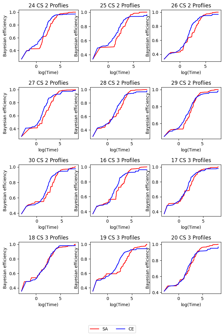
Figure 1: Bayesian $\mathcal{D}$-efficiency of designs from the CE and SA algorithms over time given the prior distribution $N(\boldsymbol{\beta}_{\boldsymbol{0}}^{S},\boldsymbol{\Sigma}_{\boldsymbol{0}}^{H})$

5 A Real-life Application in Software Development

We apply both the SA and CE algorithms to a real-life DCE used in the development of the JMP software, and subsequently compare their performances. Kessels et al., (2015) introduced this DCE for generating partial profile designs, where the levels of only a subset of the attributes vary in each choice set, but the DCE also lends itself to generating full profile designs, which allow the levels of all attributes to vary, and which we aim to optimize in this research.

JMP, developed by SAS Institute, is a statistical analysis software suite for dynamic data visualization and statistical analysis. To understand users’ preferences for output displays generated by JMP, the JMP development group conducted an online DCE, where customers evaluated 15 choice sets of two output displays from a simple linear regression analysis. This DCE investigated seven attributes listed in Table 5. An example of a choice set is illustrated in Figure 2, with the levels for each attribute detailed in Table 6. The choice set contains two partial profiles that vary the levels of only three of the seven attributes. As actual regression results are being shown to respondents, and not the attribute levels themselves, it seems also feasible to present respondents with full profile designs.

Table 5: Attributes and attribute levels for the JMP graphics DCE

Attribute	Attribute levels
Report background color	Bluish	Creamish	Light gray	White
Picture background color	Contrast	Same
Graph background color	Light gray	White
Frame line color	Black	Gray
Frame all sides	No	Yes
Outer graph rectangle	No	Yes
$Y$-axis title	Horizontal above	vertical left

Figure 2: Example choice set used in the JMP graphics DCE

Table 6: Attribute levels for the two output displays of the example choice set in Figure 2

Attribute	Profile 1	Profile 2
Report background color	Creamish	Creamish
Picture background color	Contrast	Same
Graph background color	Light Gray	Light Gray
Frame line color	Black	Black
Frame all sides	No	Yes
Outer graph rectangle	No	Yes
$Y$-axis title	Vertical left	Vertical left

To obtain precise estimates, Kessels et al., (2015) generated a Bayesian $\mathcal{D}$-optimal partial profile design with 120 choice sets using the CE algorithm. Because of the lack of prior information about user preferences, they employed a naive prior distribution $N(\mathbf{0}_{9},{\bf I}_{17})$. In our study, we utilize the same prior distribution to compute Bayesian $\mathcal{D}$-optimal full profile designs comprising 120 choice sets of size 2 assuming a multinomial logit model. Consistent with the computational experiments described in Section 4, we first ran the CE algorithm with 30 different starting designs, documented its run time, and used this duration as the maximum run time for the SA algorithm to ensure comparability.

Compared to the optimal design obtained with the SA algorithm, the CE algorithm exhibits worse performance providing an optimal design with a relative $\mathcal{D}_{B}$-efficiency of 98.62%. Figure 3 illustrates the temporal Bayesian $\mathcal{D}$-efficiency of the optimal designs derived from both the CE and SA algorithms. It can be observed that the designs obtained by the CE algorithm exhibit superior performance only in the very early stages of run time. Beyond a run time of 2 seconds, the SA designs consistently outperform the CE designs. The optimal designs generated by both algorithms can be found in Appendix A for reference. Also for this application, the CE design is characterized by somewhat more attribute level overlap compared to the SA design (9.88% versus 8.10%).

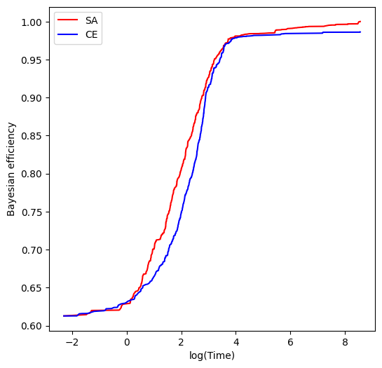
Figure 3: Bayesian $\mathcal{D}$-efficiency of designs from the CE and SA algorithms over time for the JMP graphics DCE

6 Discussion and Conclusion

In this study, we introduce the SA algorithm for the first time for the generation of Bayesian $\mathcal{D}$-optimal designs for DCEs. Our SA algorithm initiates with a random choice design. In each iteration, it randomly generates a new choice design. The algorithm not only accepts all superior designs but also, with a specific probability, less optimal designs, thus effectively preventing early convergence. Compared to the widely-used CE algorithm, our SA algorithm is more likely to obtain better designs in a shorter time frame. Our computational experiments and the real-life case study validate the superior performance of the SA algorithm across various scenarios, particularly when the prior preference information is very uncertain, or when there are more prior parameters that are large in absolute size. In such instances, due to increased uncertainty and complexity in the optimization problem, the SA algorithm’s advantage of avoiding premature convergence to local optima compared to the CE algorithm becomes more pronounced.

For future research, we suggest the following four extensions:

1. Bayesian Adaptive Designs: We employed the Bayesian optimal design approach, which outperforms other design approaches when prior information is adequate (Kessels et al.,, 2006). However, this method is prone to severe misspecifications of the prior distribution (Walker et al.,, 2018), posing challenges when prior information is insufficient, for example in the event that respondents have opposite preferences but the prior distribution does not reflect this. To address this, Yu et al., (2011) proposed a Bayesian adaptive design approach for individual respondents. This method progressively refines the prior distribution in a sequential manner for each respondent during the survey process. For future research, we also recommend the application of the SA algorithm in the construction of Bayesian adaptive designs.

2. Parameter Selection: The selection of parameters for the SA algorithm critically influences its performance, including the Cooling Function and Stopping Criterion. In this research, we chose the Hyperbolic Cooling Function, a fast annealing model that focuses on the search in the low-temperature regions (Wang and Xu,, 2020), aligning with our primary objective of enhancing the algorithm’s efficiency. For future work, we advocate the design of DCEs with various Cooling Functions and a comparative analysis of their performances. Furthermore, the Stopping Criterion controls the termination point of the SA algorithm. In our study, we utilized the maximum run time as the Stopping Criterion, offering users the flexibility to adjust the run time as needed. However, our experiments also indicate that in many instances, the SA algorithm ceases to show significant improvements after a certain run time. To address this, we suggest that future research could explore the use of an adaptive Stopping Criterion, such as terminating the algorithm after several reheating cycles without observed improvements.

3. Partial Profile Designs: Our work employs the classical random utility model that assumes that individuals tend to make compensatory decisions. However, in practical scenarios, respondents may adopt non-compensatory strategies due to the complexity of the decision-making task. An increase in the number of attributes escalates the cognitive effort required, potentially leading respondents to resort to simpler decision-making strategies, as indicated by Caussade et al., (2005). To mitigate the complexity of the comparisons and to deter respondents from adopting simpler strategies, one approach is to maintain constant levels for some attributes in every choice situation. This approach leads to a partial profile design, as discussed by Chrzan, (2010). In future research, extending the application of the SA algorithm to partial profile designs could be a significant and meaningful addition. The SA algorithm could be compared to the different CE algorithms for partial profile designs, which are described in Kessels et al., 2011a ; Kessels et al., (2015) and Palhazi Cuervo et al., (2016).

4. Choice Experiments with Mixtures: Our research primarily focuses on the design of DCEs involving categorical (specifications of the) attributes. However, instances where attributes are proportions of ingredients in a mixture have not been adequately addressed. In real-world contexts, many consumer products can be described as mixtures of ingredients. Examples include various chemicals in pesticides (Cornell,, 2011), different types of fish in fish patties (Cornell,, 1988), and diverse kinds of wheat used to bake bread (Rehman et al.,, 2007). When designing DCEs for such cases, a significant challenge arises from experimental regions that are not a simplex. Refining our SA algorithm to tackle this issue and applying it to Bayesian optimal design for DCEs involving mixtures is also a potential direction for our future research.

Appendix Appendix A. Tables

Table A1: Parameter settings of the SA algorithm for the different design cases under study

#Choice Sets	#Profiles	Prior Distribution	$\widehat{|\Delta|_{max}}$	$T_{0}$	Maximum Time (s)
24	2	$\small{N(\boldsymbol{\beta}_{\boldsymbol{0}}^{S},\boldsymbol{\Sigma}_{\boldsymbol{0}}^{H})}$	1.00	99.45	3409.0
24	2	$\small{N(\boldsymbol{\beta}_{\boldsymbol{0}}^{W},\boldsymbol{\Sigma}_{\boldsymbol{0}}^{H})}$	0.83	82.68	3543.6
24	2	$\small{N(\boldsymbol{\beta}_{\boldsymbol{0}}^{S},\boldsymbol{\Sigma}_{\boldsymbol{0}}^{L})}$	1.43	142.65	2974.2
24	2	$\small{N(\boldsymbol{\beta}_{\boldsymbol{0}}^{W},\boldsymbol{\Sigma}_{\boldsymbol{0}}^{L})}$	1.10	109.07	2784.6
24	2	$\small{N(\mathbf{0}_{17},\boldsymbol{\Sigma}_{\boldsymbol{0}}^{H})}$	0.90	89.55	3297.8
25	2	$\small{N(\boldsymbol{\beta}_{\boldsymbol{0}}^{S},\boldsymbol{\Sigma}_{\boldsymbol{0}}^{H})}$	1.34	132.94	3667.9
25	2	$\small{N(\boldsymbol{\beta}_{\boldsymbol{0}}^{W},\boldsymbol{\Sigma}_{\boldsymbol{0}}^{H})}$	0.76	75.25	3509.3
25	2	$\small{N(\boldsymbol{\beta}_{\boldsymbol{0}}^{S},\boldsymbol{\Sigma}_{\boldsymbol{0}}^{L})}$	1.78	177.57	3239.8
25	2	$\small{N(\boldsymbol{\beta}_{\boldsymbol{0}}^{W},\boldsymbol{\Sigma}_{\boldsymbol{0}}^{L})}$	0.90	89.65	2997.9
25	2	$\small{N(\mathbf{0}_{17},\boldsymbol{\Sigma}_{\boldsymbol{0}}^{H})}$	0.72	71.98	3176.6
26	2	$\small{N(\boldsymbol{\beta}_{\boldsymbol{0}}^{S},\boldsymbol{\Sigma}_{\boldsymbol{0}}^{H})}$	0.90	89.11	3404.6
26	2	$\small{N(\boldsymbol{\beta}_{\boldsymbol{0}}^{W},\boldsymbol{\Sigma}_{\boldsymbol{0}}^{H})}$	0.83	82.55	3577.2
26	2	$\small{N(\boldsymbol{\beta}_{\boldsymbol{0}}^{S},\boldsymbol{\Sigma}_{\boldsymbol{0}}^{L})}$	1.33	132.73	3261.3
26	2	$\small{N(\boldsymbol{\beta}_{\boldsymbol{0}}^{W},\boldsymbol{\Sigma}_{\boldsymbol{0}}^{L})}$	0.73	72.79	3179.9
26	2	$\small{N(\mathbf{0}_{17},\boldsymbol{\Sigma}_{\boldsymbol{0}}^{H})}$	0.80	79.14	3294.1
27	2	$\small{N(\boldsymbol{\beta}_{\boldsymbol{0}}^{S},\boldsymbol{\Sigma}_{\boldsymbol{0}}^{H})}$	1.01	100.18	3602.6
27	2	$\small{N(\boldsymbol{\beta}_{\boldsymbol{0}}^{W},\boldsymbol{\Sigma}_{\boldsymbol{0}}^{H})}$	0.81	80.17	3771.0
27	2	$\small{N(\boldsymbol{\beta}_{\boldsymbol{0}}^{S},\boldsymbol{\Sigma}_{\boldsymbol{0}}^{L})}$	1.52	150.92	3495.2
27	2	$\small{N(\boldsymbol{\beta}_{\boldsymbol{0}}^{W},\boldsymbol{\Sigma}_{\boldsymbol{0}}^{L})}$	0.96	95.26	2979.6
27	2	$\small{N(\mathbf{0}_{17},\boldsymbol{\Sigma}_{\boldsymbol{0}}^{H})}$	0.82	81.90	3313.7
28	2	$\small{N(\boldsymbol{\beta}_{\boldsymbol{0}}^{S},\boldsymbol{\Sigma}_{\boldsymbol{0}}^{H})}$	0.84	83.84	3534.8
28	2	$\small{N(\boldsymbol{\beta}_{\boldsymbol{0}}^{W},\boldsymbol{\Sigma}_{\boldsymbol{0}}^{H})}$	0.69	68.45	4005.0
28	2	$\small{N(\boldsymbol{\beta}_{\boldsymbol{0}}^{S},\boldsymbol{\Sigma}_{\boldsymbol{0}}^{L})}$	1.19	118.22	3463.7
28	2	$\small{N(\boldsymbol{\beta}_{\boldsymbol{0}}^{W},\boldsymbol{\Sigma}_{\boldsymbol{0}}^{L})}$	0.67	66.60	3285.3
28	2	$\small{N(\mathbf{0}_{17},\boldsymbol{\Sigma}_{\boldsymbol{0}}^{H})}$	0.70	70.02	3636.8
29	2	$\small{N(\boldsymbol{\beta}_{\boldsymbol{0}}^{S},\boldsymbol{\Sigma}_{\boldsymbol{0}}^{H})}$	0.89	88.78	3778.1
29	2	$\small{N(\boldsymbol{\beta}_{\boldsymbol{0}}^{W},\boldsymbol{\Sigma}_{\boldsymbol{0}}^{H})}$	0.58	57.61	4803.3
29	2	$\small{N(\boldsymbol{\beta}_{\boldsymbol{0}}^{S},\boldsymbol{\Sigma}_{\boldsymbol{0}}^{L})}$	1.15	114.61	3652.8
29	2	$\small{N(\boldsymbol{\beta}_{\boldsymbol{0}}^{W},\boldsymbol{\Sigma}_{\boldsymbol{0}}^{L})}$	0.51	51.24	3742.0
29	2	$\small{N(\mathbf{0}_{17},\boldsymbol{\Sigma}_{\boldsymbol{0}}^{H})}$	0.94	93.38	3635.2
30	2	$\small{N(\boldsymbol{\beta}_{\boldsymbol{0}}^{S},\boldsymbol{\Sigma}_{\boldsymbol{0}}^{H})}$	0.88	87.62	3898.1
30	2	$\small{N(\boldsymbol{\beta}_{\boldsymbol{0}}^{W},\boldsymbol{\Sigma}_{\boldsymbol{0}}^{H})}$	0.80	79.72	4328.1
30	2	$\small{N(\boldsymbol{\beta}_{\boldsymbol{0}}^{S},\boldsymbol{\Sigma}_{\boldsymbol{0}}^{L})}$	0.99	98.32	3854.6
30	2	$\small{N(\boldsymbol{\beta}_{\boldsymbol{0}}^{W},\boldsymbol{\Sigma}_{\boldsymbol{0}}^{L})}$	0.72	71.27	3603.0
30	2	$\small{N(\mathbf{0}_{17},\boldsymbol{\Sigma}_{\boldsymbol{0}}^{H})}$	0.56	55.90	3630.5
16	3	$\small{N(\boldsymbol{\beta}_{\boldsymbol{0}}^{S},\boldsymbol{\Sigma}_{\boldsymbol{0}}^{H})}$	1.04	103.09	3218.5
16	3	$\small{N(\boldsymbol{\beta}_{\boldsymbol{0}}^{W},\boldsymbol{\Sigma}_{\boldsymbol{0}}^{H})}$	0.83	82.13	3563.6
16	3	$\small{N(\boldsymbol{\beta}_{\boldsymbol{0}}^{S},\boldsymbol{\Sigma}_{\boldsymbol{0}}^{L})}$	1.48	147.65	3203.6
16	3	$\small{N(\boldsymbol{\beta}_{\boldsymbol{0}}^{W},\boldsymbol{\Sigma}_{\boldsymbol{0}}^{L})}$	0.70	70.06	3094.4
16	3	$\small{N(\mathbf{0}_{17},\boldsymbol{\Sigma}_{\boldsymbol{0}}^{H})}$	0.57	56.35	2947.6
17	3	$\small{N(\boldsymbol{\beta}_{\boldsymbol{0}}^{S},\boldsymbol{\Sigma}_{\boldsymbol{0}}^{H})}$	0.85	84.62	3563.7
17	3	$\small{N(\boldsymbol{\beta}_{\boldsymbol{0}}^{W},\boldsymbol{\Sigma}_{\boldsymbol{0}}^{H})}$	0.52	51.50	3550.9
17	3	$\small{N(\boldsymbol{\beta}_{\boldsymbol{0}}^{S},\boldsymbol{\Sigma}_{\boldsymbol{0}}^{L})}$	1.68	167.45	3734.2
17	3	$\small{N(\boldsymbol{\beta}_{\boldsymbol{0}}^{W},\boldsymbol{\Sigma}_{\boldsymbol{0}}^{L})}$	0.43	42.62	3313.0
17	3	$\small{N(\mathbf{0}_{17},\boldsymbol{\Sigma}_{\boldsymbol{0}}^{H})}$	0.52	52.10	3228.8
18	3	$\small{N(\boldsymbol{\beta}_{\boldsymbol{0}}^{S},\boldsymbol{\Sigma}_{\boldsymbol{0}}^{H})}$	0.70	70.03	3705.0
18	3	$\small{N(\boldsymbol{\beta}_{\boldsymbol{0}}^{W},\boldsymbol{\Sigma}_{\boldsymbol{0}}^{H})}$	0.48	47.53	3588.9
18	3	$\small{N(\boldsymbol{\beta}_{\boldsymbol{0}}^{S},\boldsymbol{\Sigma}_{\boldsymbol{0}}^{L})}$	1.04	103.39	3695.3
18	3	$\small{N(\boldsymbol{\beta}_{\boldsymbol{0}}^{W},\boldsymbol{\Sigma}_{\boldsymbol{0}}^{L})}$	0.48	47.92	3449.5
16	3	$\small{N(\mathbf{0}_{17},\boldsymbol{\Sigma}_{\boldsymbol{0}}^{H})}$	0.44	43.77	3420.3
19	3	$\small{N(\boldsymbol{\beta}_{\boldsymbol{0}}^{S},\boldsymbol{\Sigma}_{\boldsymbol{0}}^{H})}$	1.18	117.67	4505.4
19	3	$\small{N(\boldsymbol{\beta}_{\boldsymbol{0}}^{W},\boldsymbol{\Sigma}_{\boldsymbol{0}}^{H})}$	1.37	136.14	4043.2
19	3	$\small{N(\boldsymbol{\beta}_{\boldsymbol{0}}^{S},\boldsymbol{\Sigma}_{\boldsymbol{0}}^{L})}$	1.67	165.87	4178.5
19	3	$\small{N(\boldsymbol{\beta}_{\boldsymbol{0}}^{W},\boldsymbol{\Sigma}_{\boldsymbol{0}}^{L})}$	0.51	50.53	3760.9
19	3	$\small{N(\mathbf{0}_{17},\boldsymbol{\Sigma}_{\boldsymbol{0}}^{H})}$	1.40	138.90	3592.7
20	3	$\small{N(\boldsymbol{\beta}_{\boldsymbol{0}}^{S},\boldsymbol{\Sigma}_{\boldsymbol{0}}^{H})}$	0.63	62.43	5097.9
20	3	$\small{N(\boldsymbol{\beta}_{\boldsymbol{0}}^{W},\boldsymbol{\Sigma}_{\boldsymbol{0}}^{H})}$	0.50	49.41	4301.5
20	3	$\small{N(\boldsymbol{\beta}_{\boldsymbol{0}}^{S},\boldsymbol{\Sigma}_{\boldsymbol{0}}^{L})}$	1.05	104.89	4265.4
20	3	$\small{N(\boldsymbol{\beta}_{\boldsymbol{0}}^{W},\boldsymbol{\Sigma}_{\boldsymbol{0}}^{L})}$	0.47	46.69	4691.9
20	3	$\small{N(\mathbf{0}_{17},\boldsymbol{\Sigma}_{\boldsymbol{0}}^{H})}$	0.57	57.08	3840.6

Table A2: $\mathcal{D}_{B}$-optimal designs generated by the CE and SA algorithms for the JMP graphics DCE

Choice Set	CE								SA
1	1	2	2	1	1	2	2		1	2	1	1	1	1	2
1	4	1	1	2	2	1	1		3	1	2	2	2	2	2
2	3	2	2	2	1	2	1		1	2	2	2	2	2	1
2	4	1	1	1	2	1	2		3	1	1	1	1	1	2
3	3	2	1	2	2	2	1		2	2	2	1	2	2	1
3	1	1	2	1	1	1	1		1	1	1	2	1	1	1
4	4	1	1	1	2	2	1		4	2	2	2	1	1	1
4	2	2	2	2	1	1	2		3	1	1	2	2	2	2
5	1	2	1	1	1	2	2		2	1	1	1	1	1	1
5	2	1	2	2	2	1	1		1	2	2	2	1	2	2
6	1	1	2	2	1	1	2		4	2	1	1	1	1	1
6	3	2	1	1	2	2	1		2	1	2	2	2	2	1
7	2	1	1	1	1	1	2		3	2	1	2	1	1	2
7	3	2	2	2	2	2	1		4	1	2	1	2	2	2
8	2	2	2	1	1	2	2		3	2	1	1	2	2	2
8	4	1	1	2	2	1	1		1	1	2	2	1	1	1
9	1	1	2	2	2	2	1		1	2	2	1	2	1	2
9	4	2	1	1	1	1	1		3	1	1	2	1	2	1
10	1	2	2	1	2	1	1		1	2	2	1	1	2	1
10	4	1	1	2	1	2	2		4	1	1	2	2	1	2
11	3	2	2	1	2	1	2		3	2	2	1	2	1	2
11	4	1	1	2	1	2	1		1	1	1	2	1	2	1
12	4	1	2	1	1	2	1		1	2	2	1	1	2	1
12	1	2	1	2	2	1	2		3	1	1	2	2	1	2
13	1	2	1	2	2	1	1		2	1	2	1	2	1	1
13	4	1	2	1	1	2	2		1	2	1	2	1	2	2
14	3	2	1	2	2	1	2		2	1	2	1	1	2	1
14	2	1	2	1	1	2	1		3	2	1	2	2	1	2
15	3	1	1	1	2	1	2		3	1	2	1	2	1	2
15	1	2	2	2	1	2	2		2	2	1	2	1	2	1
16	1	2	2	2	2	1	2		3	2	1	2	2	1	1
16	2	1	1	1	1	1	2		1	1	2	1	1	2	2
17	3	1	2	1	1	1	1		4	1	1	1	2	1	1
17	4	2	2	2	1	2	2		2	2	2	2	1	2	2
18	2	1	2	2	1	1	2		3	2	1	1	1	2	1
18	4	2	2	1	2	1	2		2	1	2	2	2	1	2
19	4	2	1	2	2	1	2		2	2	1	2	2	1	2
19	3	1	1	2	2	2	1		1	1	2	1	1	2	1
20	2	1	2	1	2	2	2		1	1	2	2	1	1	2
20	3	2	1	2	1	1	1		3	2	1	1	2	2	1
21	2	2	1	1	1	1	1		1	1	2	1	2	1	2
21	4	1	2	2	2	1	1		3	2	1	2	1	2	1
22	2	2	2	2	2	2	2		1	2	2	1	2	1	2
22	1	1	1	1	1	1	1		4	1	1	2	1	2	1
23	2	1	1	1	1	2	2		4	2	1	2	2	2	1
23	1	2	2	2	1	2	2		3	1	1	1	2	1	2
24	1	1	1	1	2	2	1		4	1	1	1	1	2	1
24	3	2	2	2	1	1	2		3	2	2	2	2	1	2
25	2	2	2	2	2	1	1		3	1	1	1	1	2	1
25	3	1	1	1	1	1	1		2	2	2	2	1	1	2
26	3	2	1	1	2	2	2		2	1	1	2	2	1	2
26	2	1	2	2	1	1	1		3	2	2	1	1	2	1
27	2	1	1	2	1	1	2		1	2	2	2	2	2	1
27	3	2	2	1	2	2	2		4	1	1	1	1	1	1
28	2	1	2	2	1	2	2		2	2	1	1	1	2	2
28	1	2	1	1	2	1	1		3	1	2	2	2	1	1
29	3	2	2	1	1	1	1		3	2	2	2	1	1	2
29	1	1	1	2	2	2	1		2	1	1	1	2	2	1
30	1	1	2	1	2	1	2		2	2	2	2	2	2	2
30	2	2	1	2	1	2	1		4	1	1	1	1	1	1
31	1	1	2	1	2	2	1		1	1	1	1	2	2	2
31	4	2	2	1	1	1	2		2	2	2	2	2	1	1
32	1	2	2	2	1	2	2		3	1	2	1	2	1	1
32	3	1	1	1	1	1	1		1	2	1	2	1	2	2
33	3	2	2	2	2	2	2		4	1	1	1	1	2	2
33	2	1	1	1	1	1	1		2	2	2	2	2	1	1
34	2	2	1	2	2	1	2		2	2	2	1	2	1	1
34	3	1	2	1	1	2	1		3	1	1	2	1	2	2
35	3	2	2	1	2	1	1		1	1	1	1	1	1	2
35	1	1	1	2	1	2	2		3	2	2	2	2	2	1
36	1	2	1	1	1	1	1		1	1	1	1	1	1	1
36	2	1	2	2	2	1	1		3	2	2	2	2	2	2
37	3	1	2	2	1	1	2		2	2	2	1	1	2	1
37	4	2	2	2	2	2	1		4	1	1	2	2	1	2
38	1	2	1	1	2	2	2		2	1	1	2	2	2	1
38	3	1	2	2	1	1	1		1	2	2	1	1	1	1
39	1	2	1	2	1	1	2		4	2	2	2	1	1	1
39	2	1	2	1	2	2	2		3	1	1	2	1	2	2
40	3	1	1	1	2	2	2		1	1	1	2	2	1	2
40	4	2	2	1	1	1	1		3	2	2	1	1	2	1
41	1	2	2	1	2	2	2		3	1	2	1	1	1	1
41	4	1	1	2	1	1	1		1	2	1	2	2	2	1
42	3	2	2	2	1	1	1		2	2	1	1	2	2	2
42	2	1	1	1	2	2	2		3	1	2	2	1	1	1
43	2	2	2	1	1	1	1		3	1	1	2	1	1	2
43	3	1	1	2	2	2	1		4	2	2	1	2	1	2
44	3	1	2	2	1	1	2		2	2	2	1	1	2	1
44	2	2	1	1	2	2	1		4	1	1	2	2	1	2
45	3	2	1	2	1	1	2		4	1	1	1	2	2	2
45	4	1	2	1	2	2	2		1	2	2	2	1	1	1
46	4	1	1	2	1	2	2		3	1	1	2	1	2	1
46	2	2	2	1	2	1	1		4	2	2	2	1	1	2
47	2	2	2	1	2	2	1		3	2	1	1	2	1	2
47	4	1	1	2	1	1	2		1	1	2	2	1	2	1
48	2	2	2	1	1	2	1		2	1	1	2	1	2	2
48	3	1	1	2	2	1	2		3	2	2	1	2	1	1
49	3	2	1	1	1	2	2		4	1	1	1	2	2	1
49	2	1	2	2	2	1	1		1	2	2	2	1	1	2
50	4	1	2	2	1	2	1		1	1	2	2	2	1	2
50	3	2	1	1	2	1	1		2	2	1	1	1	2	1
51	3	1	1	2	2	1	1		2	1	1	1	1	1	2
51	4	2	2	2	2	2	2		3	2	2	2	2	2	1
52	4	1	2	1	2	1	2		4	1	1	2	1	1	1
52	1	2	1	2	1	2	1		3	2	2	1	2	2	2
53	1	1	2	1	1	2	1		1	2	1	1	2	1	1
53	3	2	1	2	2	1	2		3	1	2	2	1	2	2
54	2	2	1	2	1	1	2		4	1	1	1	2	1	2
54	1	1	2	1	2	2	1		3	2	2	2	1	2	1
55	2	1	1	2	2	2	2		4	2	2	1	1	2	1
55	1	2	2	1	1	1	2		2	1	1	1	1	2	1
56	4	2	1	1	2	2	2		3	2	2	1	1	2	2
56	1	1	1	1	1	1	1		1	1	1	2	2	1	1
57	1	2	1	1	1	1	1		1	2	2	2	1	1	1
57	3	1	2	2	2	2	1		2	1	1	1	1	2	2
58	3	2	1	2	1	2	2		2	2	2	1	2	1	2
58	2	1	2	1	2	1	1		4	1	1	2	1	2	1
59	1	2	2	2	1	2	1		4	2	1	1	1	2	1
59	2	1	1	1	1	1	2		3	1	2	2	2	1	2
60	1	1	2	1	1	2	2		2	1	2	1	2	1	1
60	3	2	1	2	2	1	1		3	2	1	2	1	2	2
61	3	1	2	1	1	1	1		4	2	2	2	1	1	1
61	1	2	1	2	2	2	1		2	1	2	1	1	1	1
62	2	1	1	2	2	2	2		2	2	1	1	2	2	2
62	3	2	2	1	1	1	2		4	1	2	2	1	1	1
63	2	2	1	2	2	2	1		1	1	1	2	2	2	2
63	4	1	2	1	1	1	1		2	2	2	1	1	1	2
64	3	2	2	2	2	1	2		3	2	2	1	1	1	1
64	2	1	1	1	2	2	1		4	1	1	2	2	2	1
65	3	1	2	2	1	2	2		4	1	1	1	1	2	1
65	2	2	1	1	2	1	1		2	2	2	2	2	1	2
66	2	1	1	2	2	1	1		1	1	1	1	2	1	2
66	4	2	2	2	1	2	1		2	2	2	2	1	2	2
67	1	2	1	1	2	1	2		4	1	1	2	1	2	2
67	3	1	2	2	1	2	1		3	2	2	1	2	1	1
68	3	2	2	2	1	2	2		3	2	2	2	2	2	2
68	4	1	1	1	2	1	1		2	1	1	1	1	1	1
69	1	2	2	2	1	1	2		1	2	1	2	2	1	1
69	4	1	1	1	2	2	1		2	1	2	1	1	2	2
70	1	1	2	2	2	1	1		3	2	2	2	1	1	1
70	3	2	1	1	1	2	2		1	1	1	1	2	2	2
71	3	2	2	1	1	2	2		1	2	2	2	1	2	1
71	1	1	1	2	2	1	1		2	1	1	1	2	1	1
72	1	1	2	1	2	1	1		1	1	2	2	2	1	1
72	2	2	1	2	1	2	2		4	2	1	1	1	2	2
73	2	1	2	1	2	1	2		1	2	1	1	1	2	1
73	3	2	1	2	1	2	1		3	1	2	2	2	1	2
74	3	2	1	1	1	1	1		1	2	1	2	1	2	1
74	1	1	2	2	2	1	1		4	1	2	1	2	1	2
75	2	2	2	2	1	1	1		3	1	1	1	2	1	1
75	1	1	1	1	1	1	1		4	2	2	1	1	2	1
76	1	2	1	1	1	2	1		4	2	2	1	2	1	1
76	3	1	2	2	2	1	2		1	1	1	1	2	1	1
77	2	2	1	2	2	1	1		4	1	1	2	1	2	2
77	4	1	2	1	1	2	2		1	2	2	1	2	1	1
78	3	1	2	2	2	1	1		1	2	1	2	1	1	2
78	4	2	1	1	1	2	2		3	1	2	1	2	2	1
79	3	2	2	1	1	2	1		1	2	2	2	2	2	1
79	4	1	1	2	2	1	2		4	1	1	1	1	1	1
80	1	2	2	2	2	2	2		2	1	1	2	1	1	2
80	4	1	1	1	1	1	2		1	2	2	1	2	2	2
81	4	1	1	2	2	2	2		3	1	2	1	1	1	2
81	1	2	2	1	1	1	2		4	2	2	1	2	2	1
82	1	2	2	1	2	2	1		1	2	1	1	2	1	2
82	4	1	1	2	1	1	2		2	1	2	2	1	2	1
83	2	2	1	2	1	1	1		3	2	1	2	2	2	2
83	1	1	2	1	2	2	2		4	1	2	1	1	1	2
84	2	1	1	2	2	2	2		2	2	1	1	2	2	1
84	4	2	2	2	2	1	1		1	1	2	2	1	1	2
85	4	1	1	1	1	2	1		3	2	1	2	1	1	1
85	3	2	2	2	2	1	2		2	1	2	1	2	2	2
86	2	2	2	1	2	1	2		2	2	1	2	1	1	2
86	4	1	1	2	1	2	1		1	1	2	1	2	2	1
87	4	1	2	2	2	1	1		1	1	2	2	2	2	1
87	3	2	1	1	2	1	1		2	2	1	1	1	1	1
88	4	2	1	1	1	2	1		2	1	2	1	2	2	2
88	2	1	2	2	2	1	2		1	2	1	2	1	1	1
89	4	2	1	2	2	2	1		2	1	2	2	2	1	1
89	3	1	2	1	1	2	1		3	2	1	1	1	1	1
90	3	1	1	2	1	2	2		4	2	1	2	2	2	2
90	4	2	2	1	2	2	2		3	1	2	1	1	2	2
91	3	1	1	1	2	1	2		2	2	1	2	2	2	1
91	4	2	1	2	2	2	1		3	1	2	1	1	1	1
92	3	2	2	2	2	2	1		2	1	2	2	1	1	1
92	1	1	1	1	1	1	2		1	2	1	1	2	2	2
93	1	2	1	1	1	2	1		3	1	2	1	2	2	1
93	2	1	2	2	2	1	2		4	2	2	1	1	1	2
94	3	1	1	1	1	2	2		3	2	2	2	1	2	2
94	1	2	2	2	1	1	1		4	1	1	1	2	1	1
95	4	2	2	1	2	2	1		4	2	2	2	1	1	2
95	1	1	1	1	2	1	2		2	1	2	2	2	2	1
96	1	1	1	1	1	1	2		4	1	2	1	2	1	1
96	2	2	2	2	2	2	1		2	2	1	2	1	2	2
97	4	2	1	1	2	1	1		2	2	2	2	1	1	1
97	1	1	2	2	1	2	2		4	1	1	1	2	2	2
98	2	1	2	2	1	2	2		3	1	1	2	2	2	2
98	3	2	1	1	2	1	1		2	2	2	1	1	1	2
99	3	1	1	2	2	2	1		3	2	2	2	2	1	2
99	4	2	2	2	1	1	2		1	1	1	1	2	2	1
100	1	1	1	1	1	2	2		3	1	2	2	1	2	1
100	3	2	2	2	1	1	1		2	2	1	1	2	1	2
101	3	1	1	1	1	2	1		2	2	2	2	2	2	1
101	2	2	2	2	1	1	2		1	1	1	1	1	1	2
102	2	2	2	1	1	1	1		2	1	2	2	1	1	1
102	1	1	1	2	2	2	1		4	2	1	1	2	2	1
103	1	1	2	2	1	2	1		4	1	1	1	1	2	2
103	2	2	1	1	2	1	2		3	2	2	2	2	1	1
104	4	2	2	2	2	1	2		4	1	1	2	2	1	1
104	2	1	1	2	2	2	1		1	2	2	1	1	2	2
105	2	2	1	1	2	2	2		2	2	1	2	1	1	1
105	1	1	2	2	1	1	1		3	1	2	1	2	2	2
106	1	2	1	2	1	2	2		4	1	2	2	2	2	2
106	4	1	2	1	2	1	1		2	2	1	1	1	2	2
107	1	2	1	2	2	2	1		3	2	1	2	2	2	2
107	2	1	2	1	1	1	1		1	1	2	1	1	1	2
108	3	1	1	2	1	1	1		2	2	1	2	2	1	1
108	4	2	2	1	2	1	1		4	1	2	1	1	2	2
109	2	2	2	2	1	2	1		3	2	1	1	1	2	2
109	4	1	1	1	2	1	2		2	1	2	2	2	1	1
110	2	1	1	2	2	2	2		4	2	2	2	1	1	1
110	4	2	1	1	1	1	1		3	1	2	1	1	1	1
111	4	1	2	2	2	2	2		2	2	1	2	2	1	1
111	2	2	1	1	2	2	2		4	1	2	1	1	2	2
112	2	2	1	1	1	2	1		4	1	2	2	1	1	2
112	1	1	2	2	2	1	2		1	2	1	1	2	2	1
113	3	1	2	2	2	1	1		3	2	1	2	1	1	2
113	2	2	1	1	1	2	2		1	1	2	1	2	2	2
114	1	2	1	2	1	1	2		1	1	2	1	2	1	1
114	3	1	2	1	2	2	1		2	2	1	2	1	2	2
115	1	2	1	2	1	1	1		1	1	2	2	1	2	2
115	3	1	2	1	2	2	2		4	2	1	1	2	1	1
116	4	1	1	2	1	1	1		2	1	2	2	2	1	1
116	3	2	2	1	2	2	2		1	2	1	1	1	2	2
117	3	2	2	2	2	2	2		2	1	2	2	1	2	2
117	4	1	1	1	1	1	1		3	2	1	1	2	1	1
118	2	2	2	2	2	2	1		3	2	1	1	1	1	1
118	4	1	1	1	1	1	1		4	1	2	2	1	1	1
119	2	2	2	2	1	1	1		1	2	1	2	2	2	2
119	4	1	1	1	2	2	2		4	1	2	1	1	1	2
120	4	2	1	2	1	2	2		1	2	1	2	2	1	2
120	1	1	2	1	2	1	2		4	1	2	1	1	2	1
Percent of Level Overlap	9.88%								8.10%

Appendix Appendix B. Figures

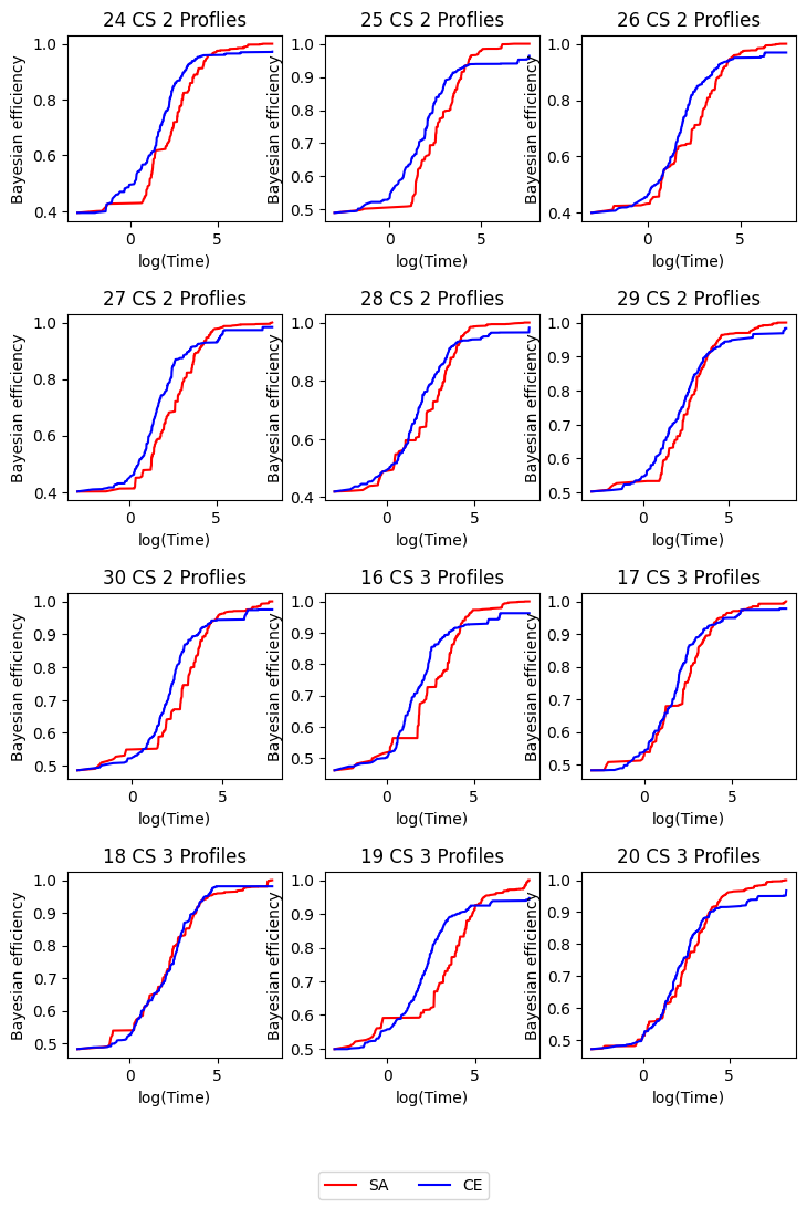
Figure B1: Bayesian $\mathcal{D}$-efficiency of designs from the CE and SA algorithms over time given the prior distribution $N(\boldsymbol{\beta}_{\boldsymbol{0}}^{W},\boldsymbol{\Sigma}_{\boldsymbol{0}}^{H})$

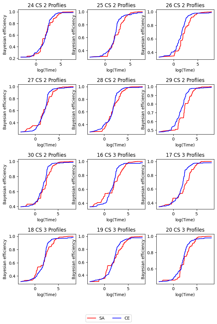
Figure B2: Bayesian $\mathcal{D}$-efficiency of designs from the CE and SA algorithms over time given the prior distribution $N(\boldsymbol{\beta}_{\boldsymbol{0}}^{S},\boldsymbol{\Sigma}_{\boldsymbol{0}}^{L})$

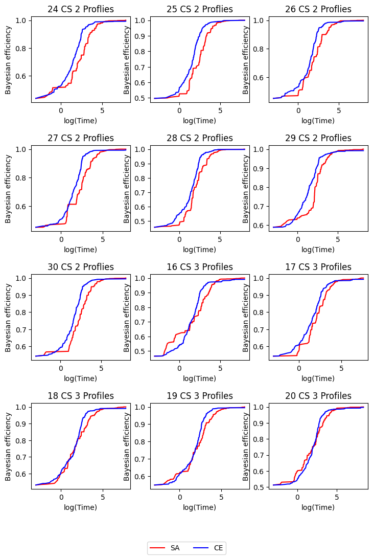
Figure B3: Bayesian $\mathcal{D}$-efficiency of designs from the CE and SA algorithms over time given the prior distribution $N(\boldsymbol{\beta}_{\boldsymbol{0}}^{W},\boldsymbol{\Sigma}_{\boldsymbol{0}}^{L})$

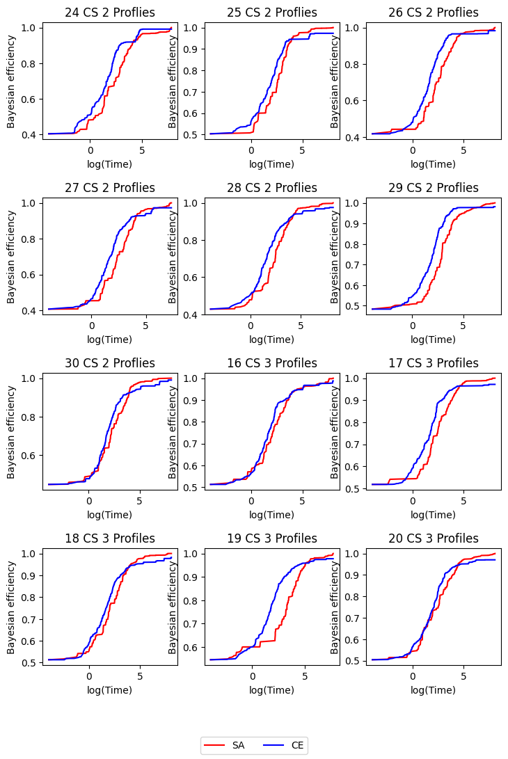
Figure B4: Bayesian $\mathcal{D}$-efficiency of designs from the CE and SA algorithms over time given the prior distribution $N(\mathbf{0}_{17},\boldsymbol{\Sigma}_{\boldsymbol{0}}^{H})$

References

- Aarts et al., (1988) Aarts, E. H., Korst, J. H., and van Laarhoven, P. J. (1988). A quantitative analysis of the simulated annealing algorithm: A case study for the traveling salesman problem. Journal of Statistical Physics, 50:187–206.
- Anagnostopoulos et al., (2006) Anagnostopoulos, A., Michel, L., Hentenryck, P. V., and Vergados, Y. (2006). A simulated annealing approach to the traveling tournament problem. Journal of Scheduling, 9:177–193.
- Angelis et al., (2001) Angelis, L., Bora-Senta, E., and Moyssiadis, C. (2001). Optimal exact experimental designs with correlated errors through a simulated annealing algorithm. Computational Statistics & Data Analysis, 37(3):275–296.
- Bohachevsky et al., (1986) Bohachevsky, I. O., Johnson, M. E., and Stein, M. L. (1986). Generalized simulated annealing for function optimization. Technometrics, 28(3):209–217.
- Burkard and Rendl, (1984) Burkard, R. E. and Rendl, F. (1984). A thermodynamically motivated simulation procedure for combinatorial optimization problems. European Journal of Operational Research, 17(2):169–174.
- Caussade et al., (2005) Caussade, S., Ortúzar, J. d. D., Rizzi, L., and Hensher, D. (2005). Assessing the influence of design dimensions on stated choice experiment estimates. Transportation Research Part B: Methodological, 39(7):621–640.
- Chrzan, (2010) Chrzan, K. (2010). Using partial profile choice experiments to handle large numbers of attributes. International Journal of Market Research, 52(6):827–840.
- Connolly, (1990) Connolly, D. T. (1990). An improved annealing scheme for the qap. European Journal of Operational Research, 46(1):93–100.
- Cook and Nachtsheim, (1980) Cook, R. D. and Nachtsheim, C. J. (1980). A comparison of algorithms for constructing exact d-optimal designs. Technometrics, 22(3):315–324.
- Cornell, (1988) Cornell, J. (1988). Analyzing data from mixture experiments containing process variables: A split-plot approach. Journal of Quality Technology, 20(1):2–23.
- Cornell, (2011) Cornell, J. (2011). A Primer on Experiments with Mixtures, volume 854. John Wiley & Sons.
- Dueck, (1993) Dueck, G. (1993). New optimization heuristics: the great deluge algorithm and the record-to-record travel. Journal of Computational Physics, 104(1):86–92.
- Franzin and Stützle, (2019) Franzin, A. and Stützle, T. (2019). Revisiting simulated annealing: A component-based analysis. Computers & Operations Research, 104:191–206.
- Geman and Geman, (1984) Geman, S. and Geman, D. (1984). Stochastic relaxation, gibbs distributions, and the bayesian restoration of images. IEEE Transactions on Pattern Analysis and Machine Intelligence, 6(6):721–741.
- Goos and Jones, (2011) Goos, P. and Jones, B. (2011). Optimal design of experiments: a case study approach. John Wiley & Sons.
- Gotwalt et al., (2009) Gotwalt, C. M., Jones, B. A., and Steinberg, D. M. (2009). Fast computation of designs robust to parameter uncertainty for nonlinear settings. Technometrics, 51(1):88–95.
- Holling and Schwabe, (2011) Holling, H. and Schwabe, R. (2011). The usefulness of bayesian optimal designs for discrete choice experiments. Applied Stochastic Models in Business and Industry, 27(3):189–192.
- Huber and Zwerina, (1996) Huber, J. and Zwerina, K. (1996). The importance of utility balance in efficient choice designs. Journal of Marketing Research, 33(3):307–317.
- Hussin and Stützle, (2014) Hussin, M. S. and Stützle, T. (2014). Tabu search vs. simulated annealing for solving large quadratic assignment instances. Computers & Operations Research, 43:286–291.
- Johnson et al., (1989) Johnson, D. S., Aragon, C. R., McGeoch, L. A., and Schevon, C. (1989). Optimization by simulated annealing: An experimental evaluation: Part i, graph partitioning. Operations Research, 37(6):865–892.
- Kessels et al., (2006) Kessels, R., Goos, P., and Vandebroek, M. (2006). A comparison of criteria to design efficient choice experiments. Journal of Marketing Research, 43(3):409–419.
- (22) Kessels, R., Jones, B., and Goos, P. (2011a). Bayesian optimal designs for discrete choice experiments with partial profiles. Journal of Choice Modelling, 4(3):52–74.
- Kessels et al., (2015) Kessels, R., Jones, B., and Goos, P. (2015). An improved two-stage variance balance approach for constructing partial profile designs for discrete choice experiments. Applied Stochastic Models in Business and Industry, 31(5):626–648.
- Kessels et al., (2008) Kessels, R., Jones, B., Goos, P., and Vandebroek, M. (2008). Recommendations on the use of bayesian optimal designs for choice experiments. Quality and Reliability Engineering International, 24(6):737–744.
- Kessels et al., (2009) Kessels, R., Jones, B., Goos, P., and Vandebroek, M. (2009). An efficient algorithm for constructing bayesian optimal choice designs. Journal of Business and Economic Statistics, 27(2):279–291.
- (26) Kessels, R., Jones, B., Goos, P., and Vandebroek, M. (2011b). The usefulness of bayesian optimal designs for discrete choice experiments. Applied Stochastic Models in Business and Industry, 27(3):173–188.
- Kirkpatrick et al., (1983) Kirkpatrick, S., Gelatt Jr, C. D., and Vecchi, M. P. (1983). Optimization by simulated annealing. Science, 220(4598):671–680.
- Liu et al., (2006) Liu, A., Wang, J., Han, G., Wang, S., and Wen, J. (2006). Improved simulated annealing algorithm solving for 0/1 knapsack problem. In Sixth International Conference on Intelligent Systems Design and Applications, volume 2, pages 1159–1164. IEEE.
- Lundy and Mees, (1986) Lundy, M. and Mees, A. (1986). Convergence of an annealing algorithm. Mathematical Programming, 34(1):111–124.
- Luyten et al., (2015) Luyten, J., Kessels, R., Goos, P., and Beutels, P. (2015). Public preferences for prioritizing preventive and curative health care interventions: A discrete choice experiment. Value in Health, 18(2):224–233.
- Malek et al., (1989) Malek, M., Guruswamy, M., Pandya, M., and Owens, H. (1989). Serial and parallel simulated annealing and tabu search algorithms for the traveling salesman problem. Annals of Operations Research, 21:59–84.
- Metropolis et al., (1953) Metropolis, N., Rosenbluth, A. W., Rosenbluth, M. N., Teller, A. H., and Teller, E. (1953). Equation of state calculations by fast computing machines. The Journal of Chemical Physics, 21(6):1087–1092.
- Meyer and Nachtsheim, (1988) Meyer, R. K. and Nachtsheim, C. J. (1988). Constructing exact d-optimal experimental designs by simulated annealing. American Journal of Mathematical and Management Sciences, 8(3-4):329–359.
- Meyer and Nachtsheim, (1995) Meyer, R. K. and Nachtsheim, C. J. (1995). The coordinate-exchange algorithm for constructing exact optimal experimental designs. Technometrics, 37:60–69.
- Monahan and Genz, (1997) Monahan, J. and Genz, A. (1997). Spherical-radial integration rules for bayesian computation. Journal of the American Statistical Association, 92(438):664–674.
- Mysovskikh, (1980) Mysovskikh, I. P. (1980). The approximation of multiple integrals by using interpolatory cubature formulae. In Quantitative approximation, pages 217–243. Academic Press.
- Palhazi Cuervo et al., (2016) Palhazi Cuervo, D., Kessels, R., Goos, P., and Sörensen, K. (2016). An integrated algorithm for the optimal design of stated choice experiments with partial profiles. Transportation Research Part B: Methodological, 93A:648–669.
- Qian and Ding, (2007) Qian, F. and Ding, R. (2007). Simulated annealing for the 0/1 multidimensional knapsack problem. Numerical Mathematics: A Journal of Chinese Universities (English Series), 16(4):320.
- Rehman et al., (2007) Rehman, S., Paterson, A., and Piggott, J. (2007). Optimisation of flours for chapatti preparation using a mixture design. Journal of the Science of Food and Agriculture, 87(3):425–430.
- Rossi and Allenby, (2003) Rossi, P. E. and Allenby, G. M. (2003). Bayesian statistics and marketing. Marketing Science, 22(3):304–328.
- Ruseckaite et al., (2017) Ruseckaite, A., Goos, P., and Fok, D. (2017). Bayesian d-optimal choice designs for mixtures. Journal of the Royal Statistical Society. Series C (Applied Statistics), 66(2):363–386.
- Sándor and Wedel, (2001) Sándor, Z. and Wedel, M. (2001). Designing conjoint choice experiments using managers’ prior beliefs. Journal of Marketing Research, 38(4):430–444.
- Strenski and Kirkpatrick, (1991) Strenski, P. N. and Kirkpatrick, S. (1991). Analysis of finite length annealing schedules. Algorithmica, 6(1-6):346–366.
- Szu and Hartley, (1987) Szu, H. and Hartley, R. (1987). Fast simulated annealing. Physics Letters A, 122(3):157–162.
- Tam, (1992) Tam, K. Y. (1992). A simulated annealing algorithm for allocating space to manufacturing cells. International Journal of Production Research, 30(1):63–87.
- Train, (2009) Train, K. E. (2009). Discrete Choice Methods with Simulation. Cambridge University Press, Cambridge.
- Walker et al., (2018) Walker, J., Wang, Y., Thorhauge, M., and Ben-Akiva, M. (2018). D-efficient or deficient? a robustness analysis of stated choice experimental designs. Theory and Decision, 84(2):215–238.
- Wang and Xu, (2020) Wang, F. and Xu, F. (2020). Analysis and research of simulated annealing algorithm and parameters. In Frontier Computing: Theory, Technologies and Applications (FC 2019), volume 8, pages 1017–1026. Springer Singapore.
- Yu et al., (2010) Yu, J., Goos, P., and Vandebroek, M. (2010). Comparing different sampling schemes for approximating the integrals involved in the efficient design of stated choice experiments. Transportation Research Part B: Methodological, 44(10):1268–1289.
- Yu et al., (2011) Yu, J., Goos, P., and Vandebroek, M. (2011). Individually adapted sequential bayesian conjoint-choice designs in the presence of consumer heterogeneity. International Journal of Research in Marketing, 28(4):378–388.
- Zijlstra et al., (2019) Zijlstra, T., Goos, P., and Verhetsel, A. (2019). A mixture-amount stated preference study on the mobility budget. Transportation Research Part A: Policy and Practice, 126:230–246.