Almost device-independent certification of GME states with minimal measurements

Abstract

Device-independent certification of quantum states allows the characterization of quantum states present inside a device by making minimal physical assumptions. A major problem in this regard is to certify quantum states using minimal resources. In this work, we consider the multipartite quantum steering scenario with an arbitrary number of parties but only one of which is trusted in the sense that the measurements performed by the trusted party are known. Consequently, the self-testing scheme is almost device-independent. Importantly, all the parties can only perform two measurements each which is the minimal number of measurements required to observe any form of quantum nonlocality. Then, we propose steering inequalities that are maximally violated by three major classes of genuinely multipartite entangled (GME) states, one, graph states of arbitrary local dimension, two, Schmidt states of arbitrary local dimension, and, three, $N$-qubit generalized W states. Using the proposed inequalities, we then provide an almost device-independent certification of the above GME states.

I Introduction

Device-independent (DI) quantum information refers to a framework in quantum information theory where protocols and tasks are designed without relying on detailed knowledge or assumptions about the devices used to implement them. In other words, DI protocols aim to achieve certain quantum information processing tasks without specifying the internal workings or characteristics of the quantum devices involved. This approach is particularly valuable for enhancing security and reliability in quantum communication and computation tasks. By removing assumptions about the devices, DI protocols provide a higher level of security against potential attacks and imperfections in the devices themselves. One of the key resources in DI quantum information processing is Bell nonlocality [1, 2], which serves as a fundamental ingredient for DI tasks such as quantum cryptography [3], random number generation [4], and state and measurement certification [5, 6, 4].

The strongest DI certification scheme is referred to as self-testing [7] (see also Ref. [8]). It allows one to infer the form of the underlying quantum system solely from the observed measurement outcomes, without needing to know the details of how the measurements were performed. Recently, a lot of attention has been devoted to finding schemes to self-test bipartite quantum states [9, 10, 11, 12, 13] and multipartite quantum states [14, 15, 16, 17, 18, 19, 20, 21, 22]. In particular [20] provides a scheme to self-test any pure entangled quantum state and [21] provides a scheme to self-test any quantum state.

A major problem in this regard is to find the optimal self-testing scheme, that is, using the minimal number of measurements to certify a particular quantum state. As the self-testing schemes are based on quantum nonlocality, each party in the experiment needs to perform at least two measurements. In the bipartite regime, there are only a few schemes that utilize two measurements per party [9, 10, 12] and even fewer in the multipartite scenario [14, 18]. Moreover, in the multipartite scenario most of the schemes are devoted to quantum states that are locally qubits. The main difficulty here consists in designing a suitable Bell inequality that is maximally violated by a given multipartite entangled quantum state. The problem becomes even more complex if one wants to find a Bell inequality which involves the minimal number of two measurements per observer.

To lower the complexity, one can introduce physically motivated assumptions into the considered scenario, leading to what is known as semi-DI certification schemes. One can for instance assume that one of the parties are trusted and their measuring devices perform known measurements. Such an assumption gives rise to scenarios which are typically referred to as one-sided-device-independent (1SDI), and the key resource enabling certification in this case is a weaker form of quantum nonlocality known as quantum steering [23, 24, 25]. Recent investigations have explored the potential of such scenarios for self-testing quantum states and measurements [26, 27, 28, 29, 30, 31, 32, 33]. For this work, we utilise the framework of multipartite quantum steering introduced in [34].

We consider here a much more complicated problem of certifying genuinely multipartite entangled (GME) states shared among an arbitrary number of parties and arbitrary local dimension using minimal number of measurements, that is, two. To simplify the problem we make the aforementioned assumption that only one party is trusted, thus, making our scheme almost device-independent. Furthermore, we restrict the parties to only choose two measurements each. We then construct steering inequalities that are maximally violated by three major classes of GME states. We then prove that maximal violation of our inequalities can be used for certification of the corresponding states. Since, among the arbitrary number of parties only one is trusted, the presented results below are almost DI certificates of the quantum state. The first family of states we can certify in this way is any connected graph state of arbitrary local dimension. Graph states are highly useful in quantum information tasks [35, 36, 37, 38]. The only other known schemes to self-test graph states are restricted to local dimension two [15, 14] and three [19]. The second class of states we consider here are the Schmidt states of arbitrary local dimension, for which a self-testing method was provided in Ref. [17]. The latter, however, requires more measurements per observer and thus is not optimal as far as physical implementations are concerned. Interestingly, our scheme can also be utilized to certify two measurements with the untrusted parties to be mutually unbiased using almost no entanglement across multiple parties. Finally, we self-test the generalized $W$ state (see below for a definition) shared among an arbitrary number of parties but only with local dimension two. While self-testing methods for the standard $N$-qubit $W$ state were already introduced in Refs. [16, 17], here, by making a mild assumption that only one party is trusted, we can significantly generalize these results to a multi-parameter class of genuinely entangled states.

Before proceeding to the results, let us introduce the relevant notions required for this work.

II Preliminaries

We consider a one-sided DI (1SDI) scenario consisting of $N$-parties, namely Alice and $N-1$ Bobs, whom we refer to as $A,B_{1},\ldots,B_{N-1}$. All the parties are located in space-like separated laboratories and share a quantum state $\rho_{A\mathbf{B}}$, where we denote $\mathbf{B}\equiv B_{1}\ldots B_{N-1}$. In this sense, each one of the $N$ parties has a device to measure their share of $\rho_{A\mathbf{B}}$. Since this is a 1SDI scenario, we assume that Alice’s measurement device is trusted, i.e., her measurements are known. Yet, we do not assume that her device performs full tomography over her share of $\rho_{A\mathbf{B}}$. On the other side, the measurement devices that belong to the $N-1$ Bobs are untrusted and we treat them as “black boxes”. The scenario we just described is also referred to as local steering [39], in which the untrusted parties perform local measurements on their respective states to steer the state owned by the trusted party. In this work, we consider that the trusted party performs the measurements given by the $d-$dimensional generalization of the Pauli $Z$ and $X$ measurement

$$Z_{d}=\sum_{i=0}^{d-1}\omega^{i}|i\rangle\!\langle i|,\qquad X_{d}=\sum_{i=0}^{d-1}|i+1\rangle\!\langle i|$$ (1)

which for ease of notation will be denoted as $Z$ and $X$ respectively. Fig. 1 contains an illustration of the scenario considered here.

We denote the inputs of all the parties $A,B_{1},\ldots,B_{N-1}$ with $x,y_{1},\ldots,y_{N-1}$ respectively and the corresponding outcomes with $a,b_{1},\ldots,b_{N-1}$. For convenience, we chose the notation $\mathbf{y}\equiv y_{1},\ldots,y_{N-1}$ and $\mathbf{b}\equiv b_{1},\ldots,b_{N-1}$. Thus, the correlations in this scenario are captured by the set of probability distributions $\vec{p}=\{p(a,\mathbf{b}|x,\mathbf{{y}})\}$, where $p(a,\mathbf{b}|x,\mathbf{y})$ tells us the probability of getting outcomes $a$ and $\mathbf{b}$ given that the measurements $x$ and $\mathbf{y}$ have been performed. According to Born’s rule, the latter is expressed as

$$p(a,\mathbf{b}|x,\mathbf{y})=\mathrm{Tr}\left[\rho_{A\mathbf{B}}\left(M_{a|x}\otimes\bigotimes_{i=1}^{N-1}N^{(i)}_{b_{i}|y_{i}}\right)\right],$$ (2)

where $M_{x}=\{M_{a|x}\}_{a}$, $N_{y_{i}}^{(i)}=\{N^{(i)}_{b_{i}|y_{i}}\}_{b_{i}}$ are the measurement operators of Alice and Bobs $B_{i}$, respectively. We recall that the measurement operators $M_{a|x}$ and $N^{(i)}_{b_{i}|y_{i}}$ are positive semi-definite and sum to identity on their corresponding Hilbert spaces.

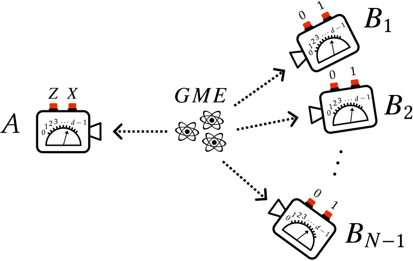
Figure 1: Depiction of the local steering scenario that we consider. A GME state is shared among $N$ parties: one Alice and $N-1$ Bobs. While Alice performs measurements $Z$ and $X$, all the other Bobs perform unknown measurements.

In our multipartite 1SDI scenario, the presence of local quantum steering is demonstrated if the probability distribution $p(a,\mathbf{b}|x,\mathbf{y})$ can not be described by a local hidden state (LHS) model [40, 39], i.e., if it can not be written as

$$p(a,\mathbf{b}|x,\mathbf{y})=\sum_{\lambda}p(\lambda)\mathrm{Tr}\left[M_{a|x}\rho_{A}^{\lambda}\right]p(\mathbf{b}|\mathbf{y},\lambda),$$ (3)

where $\lambda$ is a hidden variable that follows the probability distribution $p(\lambda)$. The hidden variable $\lambda$ determines the state $\rho^{\lambda}_{A}$ received by Alice and also the responses $p(\mathbf{b}|\mathbf{y},\lambda)$ obtained by $N-1$ Bobs. If the set of probability distributions $\{p(a,\mathbf{b}|x,\mathbf{y})\}$ can not be described by the above model, it leads to violation of a linear steering inequality, $\mathcal{B}\left[\{p(a,\mathbf{b}|x,\mathbf{y})\}\right]\leqslant\beta_{L}$, where $\mathcal{B}$ is a linear combination of $\{p(a,\mathbf{b}|x,\mathbf{y})\}$ and $\beta_{L}$ is the LHS bound , also called classical bound [41].

In this work we express steering inequalities in terms of generalized expectation values. These are defined in terms of $p(a,\mathbf{b}|x,\mathbf{y})$ as

$$\langle A_{k|x}\mathbf{B}_{\mathbf{l}|\mathbf{y}}\rangle=\sum_{a,\mathbf{b}=0}^{d-1}\omega^{ak+b_{1}l_{1}+\ldots+b_{N-1}l_{N-1}}p(a,\mathbf{b}|x,\mathbf{y}),$$ (4)

where $\mathbf{B}_{\mathbf{l}|\mathbf{y}}\equiv(B_{1})_{l_{1}|y_{1}}\ldots(B_{N-1})_{l_{N-1}|y_{N-1}}$, $\omega=\mathrm{e}^{2\pi\mathbbm{i}/d}$, and $k,l_{1},\ldots,l_{N-1}\in\{0,\ldots,d-1\}$. If the probabilities $p(a,\mathbf{b}|x,\mathbf{y})$ originate from a quantum measurement, we can write the expectation values as

$$\langle A_{k|x}\mathbf{B}_{\mathbf{l}|\mathbf{y}}\rangle=\mathrm{Tr}\left[\rho_{A\mathbf{B}}A_{x}^{k}\otimes\bigotimes_{i=1}^{N-1}(B_{i})_{l_{i}|y_{i}}\right],$$ (5)

where $A^{k}_{x}$ is the $k$-th power of the unitary observable $A_{x}$, satisfying $A_{x}^{d}=\mathbb{1}_{d}$, and $(B_{i})_{l_{i}|y_{i}}$ are the Fourier transforms of the measurement operators $N^{(i)}_{b_{i}|y_{i}}$, i.e.,

$$(B_{i})_{l_{i}|y_{i}}=\sum_{b_{i}}\omega^{b_{i}l_{i}}N^{(i)}_{b_{i}|y_{i}}.$$ (6)

In fact, since we can write $N^{(i)}_{b_{i}|y_{i}}$ as an inverse Fourier transform of $(B_{i})_{l_{i}|y_{i}}$, we can also refer to $\{(B_{i})_{l_{i}|y_{i}}\}_{l_{i}=0}^{d-1}$ as the measurements of the $i$-th Bob. Moreover, if $N_{y_{i}}^{(i)}$ are projective, then $(B_{i})_{l_{i}|y_{i}}$ are the $l_{i}$-th power of a unitary observable $B_{i,y_{i}}\coloneqq(B_{i})_{1|y_{i}}$, that is, $(B_{i})_{l_{i}|y_{i}}=\left(B_{i,y_{i}}\right)^{l_{i}}$ [13].

In what follows, we will present three classes of steering inequalities that are maximally violated by three classes of GME states, namely the $N$-qudit graph states, the $N$-qudit Schmidt states, and the generalized $N$-qubit $W$-states. Recall that a GME state is one that cannot be written as a tensor product of two other pure states corresponding to two disjoint and nonempty subsets of the parties. Formally, a GME state is a state that cannot be written in the form $|\psi\rangle_{A_{1}\ldots A_{N}}=|\alpha\rangle_{A}\otimes|\beta\rangle_{\overline{A}}$ for any bipartition $A|\overline{A}$ such that $A$ is a subset of the parties $A_{1}\ldots A_{N}$, $\overline{A}$ is the complement of $A$ and both $A$ and $\overline{A}$ are non-empty.

Maximally violating steering inequalities plays a critical role in the presented below self-testing results. When experimental results $\vec{p}$ exhibit a maximal violation, they allow us to infer both the observer’s state and the performed measurements up to local isometries. With that in mind, let us formally define multipartite 1SDI self-testing similar to the one introduced in [30]. We assume here that the measurements are projective based on dilation arguments. However, the state $\rho_{N,A\mathbf{B}}$ shared among all parties is in general mixed, which can be purified to $|\psi_{N}\rangle_{A\mathbf{B}E}$ by adding an extra system $E$ as $\rho_{N}=\mathrm{Tr}_{E}(|\psi_{N}\rangle\!\langle\psi_{N}|)$. Alice’s measurements are projective and fixed as $A_{x}$, while Bobs measurements are arbitrary and represented by $B_{i,y_{i}}$. The goal is to certify that the state shared between Alice and Bob is equivalent to a reference state $|\psi^{\prime}\rangle_{A\mathbf{B}^{\prime}}$, as well as, that the measurements performed by Bob are equivalent to the reference measurements $B_{i,y_{i}}^{\prime}$ that generates the same correlation $\vec{p}$. We say that $|\psi\rangle_{A\mathbf{B}E}$ and $B_{i,y_{i}}$ are certified by the statistics $\vec{p}$ if there exists a unitary $U_{i}:\mathcal{H}_{B_{i}}\to\mathcal{H}_{B_{i}}$ such that

$$\left(\mathbbm{1}_{A}\otimes\bigotimes_{i=1}^{N-1}U_{i}\right)|\psi_{N}\rangle_{A\mathbf{B}E} = |\psi^{\prime}\rangle_{A\mathbf{B}^{\prime}}\otimes|\phi\rangle_{\mathbf{B}^{\prime\prime}E},$$ (7a)

$$U_{i}\,B_{i,y_{i}}\,U_{i}^{\dagger} = B_{i,y_{i}}^{\prime}\otimes\mathbbm{1}_{B_{i}^{\prime\prime}},\qquad\forall i$$ (7b)

where Bobs Hilbert space is given by $\mathcal{H}_{B_{i}}=\mathcal{H}_{B_{i}^{\prime}}\otimes\mathcal{H}_{B_{i}^{\prime\prime}}$, $|\phi\rangle_{\mathbf{B}^{\prime\prime}E}$ is a junk state in $\mathcal{H}_{\mathbf{B}^{\prime\prime}}\otimes\mathcal{H}_{E}$. Let us remark here that the measurements can only be certified on the local supports of the state, thus, without loss of generality, we assume that the local supports are full-rank.

III Results

III.1 Graph states

Figure 2: Examples of graph: (a) ring graph (b) star graph corresponding to $N-$qudit GHZ state up to local unitaries.

Let us begin by defining graph states of arbitrary local dimension [42, 35, 43]. Consider a multigraph $G=(V,E,\Gamma)$ (cf. Fig. 2), where $V$ is a set of all the vertices of the graph, whereas $E$ is a set of pairs of vertices that are connected by edges. Finally, $\Gamma$ is a matrix with elements $\gamma_{i,j}=0,\ldots,d-1$ denoting the multiplicity of the edges between vertices $i$ and $j$. For our purpose, we consider graphs that are connected, that is, those in which there exist of path between any pair of vertices. Then, the graph state $|G\rangle\in(\mathbbm{C}^{d})^{\otimes N}$ corresponding to the multigraph $G=(V,E,\Gamma)$, where $N$ is the number of vertices, is constructed as:

• Each vertex of $G$ is associated the state $|+^{d}_{i}\rangle=\frac{1}{\sqrt{d}}\sum_{i=0}^{d-1}|i\rangle$ where $\{|i\rangle\}$ is the $d-$dimensional computational basis.

• For each edge $e={i,j}$ connecting the vertex $i,j$ of multiplicity $\gamma_{i,j}$, a controlled unitary

  $$Z_{i,j}^{\gamma_{i,j}}=\sum_{q=0}^{d-1}|q\rangle\!\langle q|_{i}\otimes\left(Z_{j}^{\gamma_{i,j}}\right)^{q}$$ (8)

  is applied on the state

  $$|+^{d}_{V}\rangle=\bigotimes_{i=1}^{N}|+_{i}^{d}\rangle.$$ (9)

Consequently, a graph state corresponding to the multigraphh $G=(V,E)$ is defined as

$$|G\rangle=\prod_{i,j}Z_{i,j}^{\gamma_{i,j}}|+^{d}_{V}\rangle.$$ (10)

An equivalent way to represent graph states is by using the stabilizer formalism. Given a multigraph $G=(V,E)$, let us consider a vertex $i$ and associate the operator $X$ to it. All the vertices attached by an edge $e$ to the $i-$th vertex are associated with the operator $Z$. Thus, the stabilizing operator corresponding to the $i-$th vertex is given by

$$S_{i}(G)=X_{i}\otimes\bigotimes_{j\in n(i)}Z_{j}^{\gamma_{i,j}}\qquad(i=1,2,\ldots,N),$$ (11)

where $n(i)$ is the set of vertices connected to the vertex $i$. The graph state $|G\rangle$ is the unique eigenstate of all the stabilizing operators $S_{i}(G)$ corresponding to the eigenvalue $1$. For example, the well-known Greenberger-Horne-Zeilinger (GHZ) state is a graph state.

Let us now move on to constructing steering inequalities that are maximally violated by any graph state and then use them later for self-testing. For this purpose, we construct the steering operator by considering the stabilizing operators of a graph state of the form (11). Then, we consider the first vertex, and label it as $0$ vertex, to be trusted and thus the measurement operators acting on it are known to be $Z_{d}$ and $X_{d}$ (1). Next, we replace $Z_{d}$ and $X_{d}$ on the $j$-th vertex with $B_{j,0},B_{j,1}$ respectively. The steering operator is then given by

$$\mathcal{I}_{d}(G,N) = X_{A}\otimes\bigotimes_{j\in n(0)}(B_{j,0})^{\gamma_{0,j}}$$ (12)

$$+\sum_{j\in n(0)}Z_{A}^{\gamma_{j,0}}\otimes B_{j,1}\otimes\bigotimes_{j^{\prime}\in n(j)\setminus\{0\}}(B_{j^{\prime},0})^{\gamma_{j,j^{\prime}}}$$

$$+\sum_{j\notin n(0)\cup{0}}B_{j,1}\otimes\bigotimes_{j^{\prime}\in n(j)}(B_{j^{\prime},0})^{\gamma_{j,j^{\prime}}}+h.c.,$$

where $h.c.$ denotes the Hermitian conjugate of the operator on its left-hand side with $G,N$ denoting the graph and number of vertices respectively. Notice that, given a graph $G=(V,E)$, the first term of the above operator corresponds to the stabilizer when choosing the vertex $0$, the second term consists of the stabilizers when choosing vertices connected to the $0^{\text{th}}$ vertex and the third term consists of rest of it. Also notice that in the above operator $\gamma_{i,j}=\gamma_{j,i}$ for any $i,j$. Thus, the steering inequality is given by

$$\langle\mathcal{I}_{d}(G,N)\rangle\leqslant\beta_{L},$$ (13)

where $\beta_{L}$ is the maximum value attainable using the LHS model. In Fact 1 of Appendix A, we provide an upper bound to $\beta_{L}$ in terms of a simple optimization problem that can be numerically evaluated for any graph $G$ and any $N,d$. The quantum bound $\beta_{Q}$ of the steering functional $\langle\mathcal{I}_{d}(G,N)\rangle$ is equal to the number of terms in $\mathcal{I}_{d}(G,N)$ (12), that is, $\beta_{Q}=2N$ and can be attained by the graph state $|G\rangle$ and observables $B_{j,0}=Z,B_{j,1}=X$ for any $j$. Importantly, from Fact 1 of Appendix A, we can conclude that $\beta_{L}<\beta_{Q}$ and thus the proposed steering inequality is non-trivial.

Now, if all the parties observe that $\langle\mathcal{I}_{d}(G,N)\rangle=2N$, then we can establish the following theorem.

Theorem 1.

Assume that the steering inequality (13) is maximally violated when the $0^{\text{th}}$ party Alice chooses the observables $A_{i}$ defined to be $A_{0}=Z$, $A_{1}=X$ and all the other parties choose their observables as $B_{j,i}$ for $i\in\{0,1\}$ and $j=1,2\ldots,N-1$ acting $\mathcal{H}_{B_{j}}$. Let us say that the state which attains this violation is given by $|\psi_{N}\rangle_{A\mathbf{B}E}\in\mathbbm{C}^{d}\otimes\bigotimes_{j=1}^{N-1}\mathcal{H}_{B_{j}}\otimes\mathcal{H}_{E}$, then the following statement holds true for any $d$: $\mathcal{H}_{B_{j}}=\mathcal{H}_{B^{\prime}_{j}}\otimes\mathcal{H}_{B^{\prime\prime}_{j}}$, where $\mathcal{H}_{B^{\prime}_{j}}\equiv\mathbbm{C}^{d}$, $\mathcal{H}_{B^{\prime\prime}_{j}}$ is some finite-dimensional Hilbert space, and there exists a local unitary transformation on Bob’s side $U_{j}:\mathcal{H}_{B_{j}}\rightarrow\mathcal{H}_{B_{j}}$, such that for any $j$

$$U_{j}\,B_{j,0}\,U_{j}^{\dagger}=Z_{B^{\prime}_{j}}\otimes\mathbbm{1}_{B^{\prime\prime}_{j}},\quad U_{j}\,B_{j,1}\,U_{j}^{\dagger}=X_{B^{\prime}_{j}}\otimes\mathbbm{1}_{B^{\prime\prime}_{j}}\ \$$ (14)

where ${B^{\prime\prime}}$ denotes Bob’s auxiliary system and the state $|\psi_{N}\rangle$ is given by,

$$\left(\mathbbm{1}_{AE}\otimes\bigotimes_{i=1}^{N-1}U_{j}\right)|\psi_{N}\rangle=|G\rangle_{A\mathbf{B}^{\prime}}\otimes|\xi\rangle_{\mathbf{B}^{\prime\prime}E},$$ (15)

where $|\xi\rangle_{\mathbf{B}^{\prime\prime}E}\in\bigotimes_{j=1}^{N-1}\mathcal{H}_{B_{j}^{\prime\prime}}\otimes\mathcal{H}_{E}$ denotes the auxiliary state.

The proof of the above theorem is given in Appendix A.

III.2 Schmidt states

Every pure bipartite state $|\psi\rangle_{AB}$ admits a Schmidt decomposition, that is, there exist orthonormal bases $|i\rangle_{A}$ and $|i\rangle_{B}$ in $\mathcal{H}_{A}$ and $\mathcal{H}_{B}$, respectively, such that $|\psi\rangle_{AB}=\sum_{i}\alpha_{i}|i\rangle_{A}\otimes|i\rangle_{B}$, where $\alpha_{i}>0$ and $\sum_{i}\alpha_{i}^{2}=1$. In the multipartite setting, an analogous decomposition is in general impossible. The multipartite pure states which can be represented via Schmidt decomposition are referred to as Schmidt states [17]. Under the action of local unitary operators, a multipartite Schmidt state $|\psi(\boldsymbol{\alpha})\rangle_{A\mathbf{B}}$ belonging to $\mathbb{C}^{d_{A}}\otimes\mathbb{C}^{d_{B_{1}}}\ldots\otimes\mathbb{C}^{d_{B_{N-1}}}$ can be reduced to the following form

$$|\psi(\boldsymbol{\alpha})\rangle_{A\mathbf{B}}=\sum_{i=0}^{d-1}\alpha_{i}|i\rangle^{\otimes N},$$ (16)

where $d=\min\{d_{A},d_{B_{1}},\ldots,d_{B_{N-1}}\}$ and $\boldsymbol{\alpha}\equiv\alpha_{1},\ldots,\alpha_{N}$, such that $0<\alpha_{i}<1$ for all $i$ and $\sum_{i=0}^{d-1}\alpha_{i}^{2}=1$. Because $\alpha_{i}>0$ for all $i$, the Schmidt rank of the state is maximal, which ensures that it is a $N$-qudit state.

Inspired from [31], let us now introduce a general class of steering inequalities that are maximally violated by states of the form (16) for a given $\boldsymbol{\alpha}$. For this purpose, we consider the following steering operator

$$\mathcal{S}_{d}(\boldsymbol{\alpha},N) = \sum_{k=1}^{d-1}\left[\left(\sum_{j=1}^{N-1}A_{0}^{k}\otimes B_{j,0}^{k}\right)\right.$$ (17)

$$+\left.\gamma(\boldsymbol{\alpha})A_{1}^{k}\otimes\bigotimes_{j=1}^{N-1}B_{j,1}^{k}+\delta_{k}(\boldsymbol{\alpha})A_{0}^{k}\right],$$

where the coefficients $\gamma(\boldsymbol{\alpha})$ and $\delta_{k}(\boldsymbol{\alpha})$ are given by

$$\gamma(\boldsymbol{\alpha}) = d\left[\sum_{\begin{subarray}{c}i,j=0\\ i\neq j\end{subarray}}^{d-1}\frac{\alpha_{i}}{\alpha_{j}}\right]^{-1},$$ (18)

$$\delta_{k}(\boldsymbol{\alpha}) = -\frac{\gamma(\boldsymbol{\alpha})}{d}\sum_{\begin{subarray}{c}i,j=0\\ i\neq j\end{subarray}}^{d-1}\frac{\alpha_{i}}{\alpha_{j}}\omega^{k(d-j)}.$$ (19)

In our scenario, we consider that all the $N-1$ Bobs perform two arbitrary measurements denoted by $B_{i,0}$ and $B_{i,1}$. Also, we assume that the local dimensions of the state shared by them are unknown. At the same time, because Alice’s device is trusted, her measurements are completely characterized and the local dimension of the shared state on Alice’s side is known. Alice’s observables are the generalized Pauli operators (1), that is, $A_{0}=Z_{d}$ and $A_{1}=X_{d}$.

The corresponding steering inequality is given by

$$\langle\mathcal{S}_{d}(\boldsymbol{\alpha},N)\rangle\leqslant\beta_{L}.$$ (20)

Again $\beta_{L}$ is the maximum value of $\langle\mathcal{S}_{d}(\boldsymbol{\alpha},N)\rangle$ attainable with LHS models. In Fact 3 of Appendix B, we provide a form of $\beta_{L}$ in terms of an optimization problem that can be numerically evaluated for any $d,N,\boldsymbol{\alpha}$. Then, the quantum bound $\beta_{Q}$ of $\langle\mathcal{S}_{d}(\boldsymbol{\alpha},N)\rangle$ is given by $\beta_{Q}=(d-1)(N-1)+1$ and can be attained by $|\psi(\boldsymbol{\alpha})\rangle$ and observables $B_{j,0}=Z_{d}$ and $B_{j,1}=X_{d}$ for any $j$. Importantly, from Fact 3 we can conclude that $\beta_{L}<\beta_{Q}$ and thus the proposed steering inequality is non-trivial.

Now, if all the parties observe that $\langle\mathcal{S}_{d}(\boldsymbol{\alpha},N)\rangle=(d-1)(N-1)+1$, then we can establish the following theorem.

Theorem 2.

Assume that the steering inequality (20) is maximally violated when the $0^{\text{th}}$ party Alice chooses the observables $A_{i}$ defined to be $A_{0}=Z_{d}$, $A_{1}=X_{d}$ and all the other parties choose their observables as $B_{j,i}$ for $i=0,1$ and $j=1,2\ldots,N-1$. Let us say that the state which attains this violation is given by $|\psi_{N}\rangle_{A\mathbf{B}E}\in\mathbbm{C}^{d}\otimes\bigotimes_{j=1}^{N-1}\mathcal{H}_{B_{j}}\otimes\mathcal{H}_{E}$, then the following statement holds true for any $d$: $\mathcal{H}_{B_{i}}=\mathcal{H}_{B^{\prime}_{i}}\otimes\mathcal{H}_{B^{\prime\prime}_{i}}$, where $\mathcal{H}_{B^{\prime}_{i}}\equiv\mathbbm{C}^{d}$, $\mathcal{H}_{B^{\prime\prime}_{i}}$ is some finite-dimensional Hilbert space, and there exists a local unitary transformation on Bob’s side $U_{i}:\mathcal{H}_{B_{i}}\rightarrow\mathbbm{C}^{d}\otimes\mathcal{H}_{B^{\prime\prime}_{i}}$ such that for any $i$

$$U_{i}\,B_{i,0}\,U_{i}^{\dagger}=Z_{d}\otimes\mathbbm{1}_{B^{\prime\prime}_{i}},\quad U_{i}\,B_{i,1}\,U_{i}^{\dagger}=X_{d}\otimes\mathbbm{1}_{B^{\prime\prime}_{i}},$$ (21)

where ${B^{\prime\prime}}$ denotes Bob’s auxiliary system and the state $|\psi_{N}\rangle$ is given by,

$$\left(\mathbbm{1}_{AE}\otimes\bigotimes_{i=1}^{N-1}U_{j}\right)|\psi_{N}\rangle=|\psi(\boldsymbol{\alpha})\rangle_{A\mathbf{B}^{\prime}}\otimes|\xi\rangle_{\mathbf{B}^{\prime\prime}E},$$ (22)

where $|\xi\rangle_{\mathbf{B}^{\prime\prime}E}\in\bigotimes_{j=1}^{N-1}\mathcal{H}_{B_{j}^{\prime\prime}}\otimes\mathcal{H}_{E}$ denotes the auxiliary state.

The proof of the above theorem can be found in Appendix B.

III.3 $N$-qubit generalized $W$ states

The third and last class of states that we are going to consider comprises the $N$-qubit generalized $W$ states. As the name suggests, they represent a generalization of the well-known $W$ state $|\psi_{W}\rangle=(|100\rangle+|010\rangle+|001\rangle)/\sqrt{3}$ and have the following form

$$|\psi_{W_{N}}\rangle=\sum_{l=0}^{N-1}\alpha_{l+1}|0\ldots,0,1_{l},0,\ldots,0\rangle,$$ (23)

such that $\alpha_{i}>0$ for every $i$ and $\sum_{i=1}^{N}\alpha_{i}^{2}=1$. We introduce a steering inequality that is maximally violated by the above state through the following steering operator

$$\mathcal{W}_{N}(\boldsymbol{\alpha}) = -2Z_{A}\otimes\bigotimes_{k=1}^{N-1}B_{k,0}+\sum_{l=1}^{N-1}\left[Z_{A}\otimes\mathbbm{1}_{l}\otimes\left(\mathbbm{1}-P_{l}\right)\right.$$

$$\left.+\left(\gamma_{l}X_{A}\otimes B_{l,1}+\delta_{l}Z_{A}\otimes\mathbbm{1}_{l}\right)\otimes P_{l}\right]$$

$$+\sum_{l=1}^{N-1}\left[\mathbbm{1}_{A}\otimes B_{l,0}\otimes\left(\mathbbm{1}-P_{l}\right)+\mathbbm{1}_{A}\otimes\mathbbm{1}_{l}\otimes P_{l}\right],$$

where

$$\gamma_{l}=\frac{2\alpha_{l+1}\alpha_{1}}{\alpha_{l+1}^{2}+\alpha_{1}^{2}},\quad\delta_{l}=\frac{\alpha_{l+1}^{2}-\alpha_{1}^{2}}{\alpha_{l+1}^{2}+\alpha_{1}^{2}},$$ (25)

for every $l\in\{1,\ldots,N-1\}$,

$$P_{l}=\frac{1}{2^{N-2}}\bigotimes_{k=1,k\neq l}^{N-1}\left(\mathbbm{1}_{k}+B_{k,0}\right),$$ (26)

and $B_{k,0}$ and $B_{k,1}$ are the measurements acting on the $k$-th qubit. In the same way, $\mathbbm{1}_{l}$ is the identity operation acting on the $l$-th qubit. The corresponding steering inequality is given by

$$\langle\mathcal{W}_{N}(\boldsymbol{\alpha})\rangle\leqslant\beta_{L}.$$ (27)

where $\beta_{L}$ is the LHS bound. Unfortunately, we were not able to calculate the LHS bound for this case. The quantum bound, nonetheless, is given by $\beta_{Q}=2N$ and is achieved by the state $|\psi_{W_{N}}\rangle$ and measurements $B_{j,0}=Z$ and $B_{j,1}=X$, as we prove in Fact 5 of Appendix C. By observing this value, the parties can certify the state and measurements through the following statement:

Theorem 3.

Assume that the steering inequality (27) is maximally violated when the $0^{\text{th}}$ party Alice chooses the observables $A_{i}$ defined to be $A_{0}=Z$, $A_{1}=X$ and all the other parties choose their observables as $B_{j,i}$ for $i\in\{0,1\}$ and $j=1,2\ldots,N-1$ acting $\mathcal{H}_{B_{j}}$. Let us say that the state which attains this violation is given by $|\psi_{N}\rangle_{A\mathbf{B}E}\in\mathbbm{C}^{2}\otimes\bigotimes_{j=1}^{N-1}\mathcal{H}_{B_{j}}\otimes\mathcal{H}_{E}$, then the following statement holds true: $\mathcal{H}_{B_{j}}=\mathcal{H}_{B^{\prime}_{j}}\otimes\mathcal{H}_{B^{\prime\prime}_{j}}$, where $\mathcal{H}_{B^{\prime}_{j}}\equiv\mathbbm{C}^{2}$, $\mathcal{H}_{B^{\prime\prime}_{j}}$ is some finite-dimensional Hilbert space, and there exists a local unitary transformation on Bob’s side $U_{j}:\mathcal{H}_{B_{j}}\rightarrow\mathcal{H}_{B_{j}}$, such that

$$U_{j}\,B_{j,0}\,U_{j}^{\dagger}=Z_{B^{\prime}_{j}}\otimes\mathbbm{1}_{B^{\prime\prime}_{j}},\quad U_{j}\,B_{j,1}\,U_{j}^{\dagger}=X_{B^{\prime}_{j}}\otimes\mathbbm{1}_{B^{\prime\prime}_{j}}$$ (28)

for every $j$, where ${B^{\prime\prime}}$ denotes Bob’s auxiliary system and the state $|\psi_{N}\rangle$ is given by,

$$\left(\mathbbm{1}_{AE}\otimes\bigotimes_{i=1}^{N-1}U_{j}\right)|\psi_{N}\rangle_{A\mathbf{B}E}=|\psi_{W_{N}}\rangle_{A\mathbf{B}^{\prime}}\otimes|\xi\rangle_{\mathbf{B}^{\prime\prime}E},$$ (29)

where $|\xi\rangle_{\mathbf{B}^{\prime\prime}E}\in\mathcal{H}_{B_{1}^{\prime\prime}}\otimes\ldots\otimes\mathcal{H}_{B_{N-1}^{\prime\prime}}\otimes\mathcal{H}_{E}$ denotes the auxiliary state.

The reader will find the proof for the above theorem in Appendix C.

IV Discussion

In our work, we demonstrated that although it’s very difficult to create self-testing methods with the fewest measurements possible, having trust in one of the parties makes it possible to create 1SDI schemes for many types of GME states. We focused on graph states, Schmidt states, and generalized $W$ states. Another important finding is that we can certify a pair of operators that are mutually unbiased with minimal entanglement across any number of parties in one process.

Our work raises several follow-up questions. An obvious one is how to expand our approach to certify more types of genuinely entangled multipartite states. In fact, it would be interesting to see whether the assumption considered here that one of the measurement device is trusted allows one to design certification scheme for any GME state based on the minimal number of measurements per observes. A related question that arises here is whether the ideas presented above can be combined with the results of Ref [44, 45] to design self-testing schemes for multipartite states which are based on finite statistics. What is more, it would have been interesting to explore whether the 1SDI certification scheme for graph states of any local dimension provided here could be generalized to stabilizer subspaces (cf. Ref. [46]). At the same time, as far as the experimental testing of our schemes is concerned, it is crucial to understand how resilient they are to experimental errors. Additionally, we can use our self-testing results for secure multipartite randomness generation.

V Acknowledgments

This project was funded within the QuantERA II Programme (VERIqTAS project) that has received funding from the European Union’s Horizon 2020 research and innovation programme under Grant Agreement No 101017733 and from the Polish National Science Center (project No 2021/03/Y/ST2/00175). Funded by the European Union. Views and opinions expressed are however those of the author(s) only and do not necessarily reflect those of the European Union or the European Commission. Neither the European Union nor the granting authority can be held responsible for them. This project has received funding from the European Union’s Horizon Europe research and innovation programme under grant agreement No 101080086 NeQST.

Supplementary Material: Almost device-independent certification of GME states with minimal measurements

Appendix A Appendix A: Self-testing any Graph state

Consider a connected graph $G$ with $N$ vertices and edges denoted as $e$ with their multiplicity denoted by $\gamma_{i,j}$. Then the graph state $|G\rangle$ corresponding to graph $G$ is the unique state that stabilizes the following $N$ operators

$$S(G)_{d,i}=X_{i}\otimes\bigotimes_{j\in n(i)}Z_{j}^{\gamma_{i,j}}\qquad i=1,2,\ldots,N$$ (30)

Let us now recall the steering operator introduced in the main text.

$$\mathcal{I}_{d}(G,N)=X_{A}\otimes\bigotimes_{j\in n(0)}(B_{j,0})^{\gamma_{0,j}}+\sum_{j\in n(0)}Z_{A}^{\gamma_{j,0}}\otimes B_{j,1}\otimes\bigotimes_{j^{\prime}\in n(j)\setminus\{0\}}(B_{j^{\prime},0})^{\gamma_{j,j^{\prime}}}+\sum_{j\notin n(0)\cup{0}}B_{j,1}\otimes\bigotimes_{j^{\prime}\in n(j)}(B_{j^{\prime},0})^{\gamma_{j,j^{\prime}}}+h.c.$$ (31)

where $h.c.$ denotes the Hermitian conjugate of the operator on its left-hand side. Also notice that in the above operator $\gamma_{i,j}=\gamma_{j,i}$ for any $i,j$ where $\gamma_{i,j}$ is the number of edges connecting vector $i,j$ and $n(j)$ is the set of vertices connected to $j$ vertex. The cardinality of $n(j)$ is denoted as $\overline{n}_{j}$. Now, the steering inequality is given by

$$\langle\mathcal{I}_{d}(G,N)\rangle\leqslant\beta_{L}.$$ (32)

The classical bound $\beta_{L}$ is given below.

Fact 1.

The local hidden state (LHS) bound $\beta_{L}$ of the steering functional $\langle\mathcal{I}_{d}(G,N)\rangle$ where $\mathcal{I}_{d}(G,N)$ is given in (31) is upper bounded by

$$\beta_{L}\leqslant\max_{\rho}\left(2|\langle X_{A}\rangle_{\rho}|+2\sum_{j\in n(0)}|\langle Z_{A}^{\gamma_{j,0}}\rangle_{\rho}|\right)+2(N-\overline{n}_{0}-1)$$ (33)

where $Z$ and $X$ are given in eq. (1). Furthermore, $\beta_{L}<2N$.

Proof.

As shown in [30], for any LHS model with trusted Alice, the expectation values of the joint observables take the form

$$\langle A^{k}_{x}\otimes B^{l}_{y}\rangle_{LHS}=\sum_{\lambda}p(\lambda)\langle A^{k}_{x}\rangle_{\rho_{\lambda}}\langle B^{l}_{y}\rangle_{\lambda}.$$ (34)

Consequently, we can express the steering inequality $\langle\mathcal{I}_{d}(G,N)\rangle$, where $\mathcal{I}_{d}(G,N)$ is given in (31), for any LHS model as

$$\langle\mathcal{I}_{d}(G,N)\rangle_{LHS}=\sum_{\lambda}p(\lambda)\langle\mathcal{I}_{d}(G,N)\rangle_{\lambda,LHS},$$ (35)

where $\langle\mathcal{I}_{d}(G,N)\rangle_{\lambda,LHS}$ is

$$\langle\mathcal{I}_{d}(G,N)\rangle_{\lambda,LHS}=\langle X_{A}\rangle_{\rho_{\lambda}}\langle\bigotimes_{j\in n(0)}(B_{j,0})^{\gamma_{0,j}}\rangle_{{\lambda}}+\sum_{j\in n(0)}\langle Z_{A}^{\gamma_{j,0}}\rangle_{\rho_{\lambda}}\langle B_{j,1}\otimes\bigotimes_{j^{\prime}\in n(j)\setminus\{0\}}(B_{j^{\prime},0})^{\gamma_{j,j^{\prime}}}\rangle_{{\lambda}}$$

$$+\sum_{j\notin n(0)\cup{0}}\langle B_{j,1}\rangle_{\rho_{\lambda}}\langle\bigotimes_{j^{\prime}\in n(j)}(B_{j^{\prime},0})^{\gamma_{j,j^{\prime}}}\rangle_{{\lambda}}+\langle h.c\rangle_{LHS}.\qquad$$ (36)

As $\langle B^{l}_{y}\rangle_{\lambda}\leq 1$, we obtain that

$$\langle\mathcal{I}_{d}(G,N)\rangle_{LHS}\leqslant\sum_{\lambda}p(\lambda)\left(2|\langle X_{A}\rangle_{\rho_{\lambda}}|+2\sum_{j\in n(0)}|\langle Z_{A}^{\gamma_{j,0}}\rangle_{\rho_{\lambda}}|\right)+2(N-\overline{n}_{0}-1),$$ (37)

which can be upper bounded as

$$\langle\mathcal{I}_{d}(G,N)\rangle_{LHS}\leqslant\sum_{\lambda}p(\lambda)\max_{\rho}\left(2|\langle X_{A}\rangle_{\rho}|+2\sum_{j\in n(0)}|\langle Z_{A}^{\gamma_{j,0}}\rangle_{\rho}|\right)+2(N-\overline{n}_{0}-1).$$ (38)

By using the fact that $\sum_{\lambda}p(\lambda)=1$, the above finally gives us

$$\langle\mathcal{I}_{d}(G,N)\rangle_{LHS}\leqslant\max_{\rho}\left(2|\langle X_{A}\rangle_{\rho}|+2\sum_{j\in n(0)}|\langle Z_{A}^{\gamma_{j,0}}\rangle_{\rho}|\right)+2(N-\overline{n}_{0}-1).$$ (39)

One can numerically evaluate the above quantity for any $d$ and any graph. Let us finally observe from the above expression that the LHS bound of the steering functional $\mathcal{I}_{d}(G,N)$ satisfies $\beta_{L}<2N$ because $Z$ and $X$ are mutually incompatible and there is no quantum state that can simultaneously stabilize $Z$ and $X$. ∎

Let us now compute the quantum bound of the steering functional $\langle\mathcal{I}_{d}(G,N)\rangle$.

Fact 2.

The quantum bound of the steering functional $\langle\mathcal{I}_{d}(G,N)\rangle$ where $\mathcal{I}_{d}(G,N)$ is given in (31) is given by $\beta_{Q}=2N$ and is achieved by the graph state $|G\rangle$ with the observables

$$B_{j,0}=Z,\qquad B_{j,1}=X.$$ (40)

Proof.

Let us first observe that the number of terms in the steering operator (31) is equal to twice the number of stabilizers $S(G)_{d,i}$ (11), that is, $2N$. Since the expectation value of each term is upper-bounded by $1$, thus, we have that $\langle\mathcal{I}_{d}(G,N)\rangle\leq 2N$.

Consider now that the unknown observables $B_{i,j}$ are given by

$$B_{j,0}=Z,\qquad B_{j,1}=X$$ (41)

along with the graph state $|G\rangle$, the state that is uniquely stabilized by the $S(G)_{i}$ operators. It is straightforward to observe that using these states and observables one can attain the quantum bound. ∎

Now notice that the steering operator consists $2N$ terms and consequently, the algebraic bound of $\langle\mathcal{I}_{d}(G,N)\rangle$ is also $2N$ as all the operators $B^{\dagger}_{i,j}B_{i,j}=\mathbbm{1}$. Thus, it is necessary that any state $|\psi_{N}\rangle$ and observables $B_{i,j}$ that achieves the quantum bound must satisfy the following conditions

$$\langle\psi_{N}|\overline{S}(G)_{i}|\psi_{N}\rangle=1,\qquad i={1,2,\ldots,N},$$ (42)

where $\overline{S}(G)_{i}$ represents each term of the steering operator (31). Now, using Cauchy-Schwarz inequality, one can conclude from here that

$$\forall i\qquad\overline{S}(G)_{i}|\psi_{N}\rangle=|\psi_{N}\rangle.$$ (43)

The above condition would be extremely useful for certifying any graph state. Let us now establish the following theorem.

Theorem 1.

Assume that the steering inequality (32) is maximally violated when the $0^{\text{th}}$ party Alice chooses the observables $A_{i}$ defined to be $A_{0}=Z$, $A_{1}=X$ and all the other parties choose their observables as $B_{j,i}$ for $i\in\{0,1\}$ and $j=1,2\ldots,N-1$ acting $\mathcal{H}_{B_{j}}$. Let us say that the state which attains this violation is given by $|\psi_{N}\rangle_{A\mathbf{B}}\in\mathbbm{C}^{d}\otimes\bigotimes_{j=1}^{N-1}\mathcal{H}_{B_{j}}\otimes\mathcal{H}_{E}$, then the following statement holds true for any $d$: $\mathcal{H}_{B_{j}}=\mathcal{H}_{B^{\prime}_{j}}\otimes\mathcal{H}_{B^{\prime\prime}_{j}}$, where $\mathcal{H}_{B^{\prime}_{j}}\equiv\mathbbm{C}^{d}$, $\mathcal{H}_{B^{\prime\prime}_{j}}$ is some finite-dimensional Hilbert space, and there exists a local unitary transformation on Bob’s side $U_{j}:\mathcal{H}_{B_{j}}\rightarrow\mathcal{H}_{B_{j}}$, such that

$$\forall j,\quad U_{j}\,B_{j,0}\,U_{j}^{\dagger}=Z_{B^{\prime}_{j}}\otimes\mathbbm{1}_{B^{\prime\prime}_{j}},\qquad U_{j}\,B_{j,1}\,U_{j}^{\dagger}=X_{B^{\prime}_{j}}\otimes\mathbbm{1}_{B^{\prime\prime}_{j}}$$ (44)

where ${B^{\prime\prime}}$ denotes Bob’s auxiliary system and the state $|\psi_{N}\rangle$ is given by,

$$\left(\mathbbm{1}_{AE}\otimes\bigotimes_{i=1}^{N-1}U_{j}\right)|\psi_{N}\rangle_{A\mathbf{B}E}=|G\rangle_{A\mathbf{B}^{\prime}}\otimes|\xi\rangle_{\mathbf{B}^{\prime\prime}E},$$ (45)

where $|\xi\rangle_{\mathbf{B}^{\prime\prime}E}\in\bigotimes_{j=1}^{N-1}\mathcal{H}_{B_{j}^{\prime\prime}}\otimes\mathcal{H}_{E}$ denotes the auxiliary state.

Proof.

Let us begin by considering the first term and second term of the steering operator $\eqref{graphsteeop}$ corresponding to the stabilizers when choosing the $0^{\text{th}}$ vertex and vertices connected to it respectively. As concluded in Eq. (43), we have that

$$X_{A}\otimes\bigotimes_{j\in n(0)}(B_{j,0})^{\gamma_{0,j}}|\psi_{N}\rangle=|\psi_{N}\rangle,$$ (46)

and

$$Z_{A}^{\gamma_{j,0}}\otimes B_{j,1}\otimes\bigotimes_{j^{\prime}\in n(j)\setminus\{0\}}(B_{j^{\prime},0})^{\gamma_{j,j^{\prime}}}|\psi_{N}\rangle=|\psi_{N}\rangle\qquad\forall j\in n(0).$$ (47)

Let us now choose a particular $k\in n(0)$ and rewrite the above conditions as,

$$X_{A}\otimes(B_{k,0})^{\gamma_{0,k}}\otimes\bigotimes_{j\in n(0)\setminus\{k\}}(B_{j,0})^{\gamma_{0,j}}|\psi_{N}\rangle=|\psi_{N}\rangle,$$ (48)

and

$$Z_{A}^{\gamma_{k,0}}\otimes B_{k,1}\otimes\bigotimes_{j^{\prime}\in n(k)\setminus\{0\}}(B_{j^{\prime},0})^{\gamma_{k,j^{\prime}}}|\psi_{N}\rangle=|\psi_{N}\rangle.$$ (49)

Since the observables $X$ and $Z$ are unitary and $\gamma_{0,k}=\gamma_{k,0}$, we have that

$$(B_{k,0})^{\gamma_{0,k}}\otimes\bigotimes_{j\in n(0)\setminus\{k\}}(B_{j,0})^{\gamma_{0,j}}|\psi_{N}\rangle=X_{A}^{-1}|\psi_{N}\rangle$$ (50)

and

$$B_{k,1}\otimes\bigotimes_{j^{\prime}\in n(k)\setminus\{0\}}(B_{j^{\prime},0})^{\gamma_{k,j^{\prime}}}|\psi_{N}\rangle=Z_{A}^{-\gamma_{0,k}}|\psi_{N}\rangle.$$ (51)

Now, multiplying $Z_{A}^{-\gamma_{0,k}}$ to the condition (50) and then using Eq. (51), we get that

$$(B_{k,0})^{\gamma_{0,k}}B_{k,1}\otimes\left(\bigotimes_{j\in n(0)\setminus\{k\}}(B_{j,0})^{\gamma_{0,j}}\right)\left(\bigotimes_{j^{\prime}\in n(k)\setminus\{0\}}(B_{j^{\prime},0})^{\gamma_{k,j^{\prime}}}\right)|\psi_{N}\rangle=Z_{A}^{-\gamma_{0,k}}X_{A}^{-1}|\psi_{N}\rangle.$$ (52)

Then, multiplying $X_{A}^{-1}$ to the condition (51) and then using Eq. (50), we get that

$$B_{k,1}(B_{k,0})^{\gamma_{0,k}}\otimes\left(\bigotimes_{j^{\prime}\in n(k)\setminus\{0\}}(B_{j^{\prime},0})^{\gamma_{k,j^{\prime}}}\right)\left(\bigotimes_{j\in n(0)\setminus\{k\}}(B_{j,0})^{\gamma_{0,j}}\right)|\psi_{N}\rangle=X_{A}^{-1}Z_{A}^{-\gamma_{0,k}}|\psi_{N}\rangle.$$ (53)

Notice, that terms inside the large brackets in both the above formulas commute. Now, by using the fact that $\omega^{\gamma_{0,k}}Z_{A}^{-\gamma_{0,k}}X_{A}^{-1}=X_{A}^{-1}Z_{A}^{-m_{e,k0}}$, we can multiply (52) by $\omega^{\gamma_{0,k}}$ and subtract (53) to obtain that

$$\left(\omega^{\gamma_{0,k}}(B_{k,0})^{\gamma_{0,k}}B_{k,1}-B_{k,1}(B_{k,0})^{\gamma_{0,k}}\right)\otimes\left(\bigotimes_{j\in n(0)\setminus\{k\}}(B_{j,0})^{\gamma_{0,j}}\right)\left(\bigotimes_{j^{\prime}\in n(k)\setminus\{0\}}(B_{j^{\prime},0})^{\gamma_{k,j^{\prime}}}\right)|\psi_{N}\rangle=0.$$ (54)

As the terms inside the large brackets in the above expression are unitary and thus invertible, we arrive at a simple condition

$$\left(\omega^{\gamma_{0,k}}(B_{k,0})^{\gamma_{0,k}}B_{k,1}-B_{k,1}(B_{k,0})^{\gamma_{0,k}}\right)\otimes\mathbbm{1}_{A\mathbf{B}E\setminus\{B_{k}\}}|\psi_{N}\rangle=0.$$ (55)

By taking a partial trace over all the subsystems except the $k^{\text{th}}$ one, we get that

$$\left(\omega^{\gamma_{0,k}}(B_{k,0})^{\gamma_{0,k}}B_{k,1}-B_{k,1}(B_{k,0})^{\gamma_{0,k}}\right)\rho_{k,N}=0,$$ (56)

where $\rho_{k,N}=\mathrm{Tr}_{A\mathbf{B}E\setminus\{B_{k}\}}(|\psi_{N}\rangle\!\langle\psi_{N}|)$. As discussed before, the local states of each party are full-rank and thus invertible. Consequently, we finally have that

$$\omega^{\gamma_{0,k}}(B_{k,0})^{\gamma_{0,k}}B_{k,1}=B_{k,1}(B_{k,0})^{\gamma_{0,k}}.$$ (57)

As proven in [13], if two unitary observables $B_{k,0}$ and $B_{k,1}$, for which $B_{k,0}^{d}=B_{k,1}^{d}=\mathbbm{1}$, satisfy relation (57), then there exists a unitary $U_{k}:\mathcal{H}_{B_{k}}\rightarrow\mathcal{H}_{B_{k}}$ such that

$$\quad U_{k}\,B_{k,0}\,U_{k}^{\dagger}=Z_{B^{\prime}_{k}}\otimes\mathbbm{1}_{B^{\prime\prime}_{k}},\qquad U_{k}\,B_{k,1}\,U_{k}^{\dagger}=X_{B^{\prime}_{k}}\otimes\mathbbm{1}_{B^{\prime\prime}_{k}}.$$ (58)

Similarly, we can reach the above conclusion for any vertex $j\in n(0)$. Using these derived observables, we then find the observables for vertices connected with any vertex $j\in n(0)$ in exactly the same manner as done above. Since any vertex is connected to at least one other vertex, we continue this until all the observables are found and we get that

$$U_{j}\,B_{j,0}\,U_{j}^{\dagger}=Z_{B^{\prime}_{j}}\otimes\mathbbm{1}_{B^{\prime\prime}_{j}},\qquad U_{j}\,B_{j,1}\,U_{j}^{\dagger}=X_{B^{\prime}_{j}}\otimes\mathbbm{1}_{B^{\prime\prime}_{j}}\qquad\forall j.$$ (59)

Let us now characterize the state $|\psi_{N}\rangle$ that achieves the quantum bound of the steering functional $\langle\mathcal{I}_{d}(G,N)\rangle$ (31). Notice now that by putting into the condition (43) the derived observables from (59), we get that

$$\forall i\qquad\overline{S}(G)_{i}|\psi_{N}\rangle=\left(\bigotimes_{i=1}^{N-1}U_{j}^{\dagger}\right)S(G)_{d,i,AB_{1}^{\prime\prime}\ldots B_{N}^{\prime\prime}}\otimes\mathbbm{1}_{B_{1}^{\prime\prime}\ldots B_{N}^{\prime\prime}E}\left(\bigotimes_{i=1}^{N-1}U_{j}\right)|\psi_{N}\rangle=|\psi_{N}\rangle,$$ (60)

where $S(G)_{d,i}$ are the stabilizing operators of a graph state $|G\rangle$ of the form (11). As discussed above, the graph state $|G\rangle$ is the unique eigenstate of such operators with eigenvalue $1$. Consequently, we have that

$$\left(\bigotimes_{i=1}^{N-1}U_{j}\right)|\psi_{N}\rangle_{A\mathbf{B}E}=|G\rangle_{A\mathbf{B}^{\prime}}\otimes|\xi\rangle_{\mathbf{B}^{\prime\prime}E},$$ (61)

where $|\xi\rangle_{\mathbf{B}^{\prime\prime}E}\in\bigotimes_{j=1}^{N-1}\mathcal{H}_{B_{j}^{\prime\prime}}\otimes\mathcal{H}_{E}$ denotes the auxiliary state. ∎

Appendix B Appendix B: Self-testing Schmidt states

The Schmidt states we consider have the form

$$|\psi(\boldsymbol{\alpha})\rangle_{A\mathbf{B}}=\sum_{i=0}^{d-1}\alpha_{i}|i\rangle^{\otimes N},$$ (62)

where $d=\min\{d_{A},d_{B_{i}}\}$ and $\boldsymbol{\alpha}$ is a vector composed of the Schmidt coefficients $\alpha_{i}$, such that $0<\alpha_{i}<1$ for all $i$ and $\sum_{i=0}^{d-1}\alpha_{i}^{2}=1$. Next, we are going to introduce a steering operator that provides an inequality maximally violated by states of the form (62).

Let us now recall the steering operator for Schmidt states introduced in the main text:

$$\mathcal{S}_{d}(\boldsymbol{\alpha},N)=\sum_{k=1}^{d-1}\left[\left(\sum_{j=1}^{N-1}A_{0}^{k}\otimes B_{j,0}^{k}\right)+\gamma(\boldsymbol{\alpha})A_{1}^{k}\otimes\bigotimes_{j=1}^{N-1}B_{j,1}^{k}+\delta_{k}(\boldsymbol{\alpha})A_{0}^{k}\right],$$ (63)

where

$$\gamma(\boldsymbol{\alpha})=\frac{d}{\sum_{\begin{subarray}{c}i,j=0\\ i\neq j\end{subarray}}^{d-1}\frac{\alpha_{i}}{\alpha_{j}}},\quad\delta_{k}(\boldsymbol{\alpha})=-\frac{\gamma(\boldsymbol{\alpha})}{d}\sum_{\begin{subarray}{c}i,j=0\\ i\neq j\end{subarray}}^{d-1}\frac{\alpha_{i}}{\alpha_{j}}\omega^{k(d-j)}.$$ (64)

In our scenario, we consider that all the $N-1$ Bobs perform two arbitrary measurements denoted by $B_{i_{0}}$ and $B_{i_{1}}$. Also, we assume that the local dimensions of the state they share are unknown. At the same time, because Alice’s device is trusted, her measurements are completely characterized and the local dimension of the shared state on Alice’s side is known. Alice’s observables are the generalized Pauli $Z$ and $X$ operators

$$Z_{d}=\sum_{i=0}^{d-1}\omega^{i}|i\rangle\langle i|,\qquad X_{d}=\sum_{i=0}^{d-1}|i+1\rangle\langle i|.$$ (65)

The corresponding steering inequality is given by

$$\langle\mathcal{S}_{d}(\boldsymbol{\alpha},N)\rangle\leqslant\beta_{L}$$ (66)

where $\beta_{L}$ is the LHS bound given below.

Fact 3.

The local hidden state (LHS) bound $\beta_{L}$ of the steering functional $\langle S_{d}(\boldsymbol{\alpha})\rangle$ where $S_{d}(\boldsymbol{\alpha})$ is given in (63) is upper bounded by

$$\beta_{L}\leqslant\max_{\begin{subarray}{c}|\eta_{0}|,\ldots,|\eta_{d-1}|\\ |\eta_{0}|^{2}+\ldots+|\eta_{d-1}|^{2}=1\end{subarray}}\left(d(N-1)\max_{a}{|\eta_{a}|^{2}}+\gamma(\boldsymbol{\alpha})\left[\left(\sum_{i=0}^{d-1}|\eta_{i}|\right)^{2}-\sum_{i=0}^{d-1}\alpha_{i}\sum_{a=0}^{d-1}\frac{|\eta_{a}|^{2}}{\alpha_{a}}\right]\right)-(N-2).$$ (67)

Furthermore, $\beta_{L}<(d-1)(N-1)+1$.

Proof.

In order to determine the LHS bound $\beta_{L}$ of the inequality in Eq. (63), we first express the functional $\mathcal{S}_{d}(\boldsymbol{\alpha},N)$ in the probability picture as following

$$S_{d}(\boldsymbol{\alpha})=\ d\sum_{j=1}^{N-1}\sum_{a,b_{j}=0}^{d-1}c_{a,b_{j}}p(a,b_{j}|0,0)+\gamma(\boldsymbol{\alpha})\left(d\sum_{a,\mathbf{b}=0}^{d-1}c_{a,\mathbf{b}}p(a,\mathbf{b}|1,1,\ldots,1)-\sum_{\begin{subarray}{c}i,a=0\\ i\neq a\end{subarray}}^{d-1}\alpha_{i}\frac{p(a|0)}{\alpha_{a}}\right)$$

$$-(N-1)-\gamma(\boldsymbol{\alpha})-\delta_{0}(\boldsymbol{\alpha}),$$ (68)

where $c_{a,b}=1$ if $a\oplus_{d}b=0$ and 0 otherwise, where $\oplus_{d}$ is the addition modulo $d$. Also, $c_{a,\mathbf{b}}=1$ if $a\oplus_{d}b_{1}\oplus_{d}\ldots\oplus_{d}b_{N-1}=0$ and 0 otherwise. We implement this notation because $\sum_{k=0}^{d-1}\omega^{kn(a-b)}=d\delta_{a,b}$ for any $n$. Likewise, $\sum_{k=0}^{d-1}\omega^{k(d+a-b)}=d\delta_{a,b}$. We note, from Eq. (64) that $\delta_{0}(\boldsymbol{\alpha})=-1$, which results in

$$S_{d}(\boldsymbol{\alpha})=\ d\sum_{j=1}^{N-1}\sum_{a,b_{j}=0}^{d-1}c_{a,b_{j}}p(a,b_{j}|0,0)+\gamma(\boldsymbol{\alpha})\left(d\sum_{a,\mathbf{b}=0}^{d-1}c_{a,\mathbf{b}}p(a,\mathbf{b}|1,1,\ldots,1)-\sum_{i=0}^{d-1}\alpha_{i}\sum_{a=0}^{d-1}\frac{p(a|0)}{\alpha_{a}}\right)-(N-2),$$ (69)

We consider the LHS model in which the correlations are given as

$$p(a,\mathbf{b}|x,\mathbf{y})=\sum_{\lambda\in\Lambda}p(\lambda)p(a|x,\rho^{\lambda}_{A})p(\mathbf{b}|\mathbf{y},\lambda),$$ (70)

where $\Lambda$ is some set of hidden variables $\lambda$ shared between Alice and all the Bobs with probability distribution $p(\lambda)$, whereas $p(a|x,\rho^{\lambda}_{A})$ and $p(\mathbf{b}|\mathbf{y},\lambda)$ are local probability distributions. Recall that Alice’s distributions are quantum and depend on the hidden state $\rho^{\lambda}_{A}$. The LHS model transforms our steering functional as

$$S_{d}(\boldsymbol{\alpha})= d\sum_{j=1}^{N-1}\sum_{a=0}^{d-1}\sum_{\lambda\in\Lambda}p(\lambda)p(a|0,\rho^{\lambda}_{A})p(d-a|0,\lambda)+\gamma(\boldsymbol{\alpha})\Biggl{(}d\sum_{a=0}^{d-1}\sum_{\lambda\in\Lambda}p(\lambda)p(a|1,\rho^{\lambda}_{A})p(\mathbf{b}|1,\ldots,1,\lambda)$$

$$-\sum_{i=0}^{d-1}\alpha_{i}\sum_{a=0}^{d-1}\frac{p(a|0,\rho_{A})}{\alpha_{a}}\Biggr{)}-(N-2),$$ (71)

where $b_{j}=d-a$ for every $j$ in the first term, $a\oplus_{d}b_{1}\oplus_{d}\ldots\oplus_{d}b_{N-1}=0$ in the second term, and in the last term we have used the fact that Alice’s distributions are quantum and substituted $\rho_{A}=\sum_{\lambda}\rho^{\lambda}_{A}$. Now, we note that the first two terms in the above expression are bounded from above in the following way

$$\sum_{a=0}^{d-1}\sum_{\lambda\in\Lambda}p(\lambda)p(a|0,\rho^{\lambda}_{A})p(d-a|0,\lambda)\leqslant\sum_{\lambda\in\Lambda}p(\lambda)\max_{a}{p(a|0,\rho^{\lambda}_{A})}\leqslant\max_{|\psi\rangle\in\mathcal{C}^{d}}\max_{a}{p(a|0,|\psi\rangle)},$$

$$\sum_{a=0}^{d-1}\sum_{\lambda\in\Lambda}p(\lambda)p(a|1,\rho^{\lambda}_{A})p(\mathbf{b}|1,\ldots,1,\lambda)\leqslant\sum_{\lambda\in\Lambda}p(\lambda)\max_{a}{p(a|1,\rho^{\lambda}_{A})}\leqslant\max_{|\psi\rangle\in\mathcal{C}^{d}}\max_{a}{p(a|1,|\psi\rangle)},$$ (72)

where to get the first inequalities in both cases we used the fact that probabilities are normalized. To get the second inequality we exploit the fact that Alice’s probability distributions are quantum and hence linear functions of the state. Substituting this in our function, we get

$$S_{d}(\boldsymbol{\alpha})\leqslant\max_{\psi\in\mathcal{C}^{d}}\left[d(N-1)\max_{a}{p(a|0,|\psi\rangle)}+\gamma(\boldsymbol{\alpha})\left(d\max_{a}p(a|1,|\psi\rangle)-\sum_{i=0}^{d-1}\alpha_{i}\sum_{a=0}^{d-1}\frac{p(a|0,|\psi\rangle)}{\alpha_{a}}\right)\right]-(N-2),$$ (73)

where we have used the fact that the maximization over the state $|\psi\rangle$ is happening over the whole expression. We can further write the state $|\psi\rangle$ in the computational basis as $|\psi\rangle=\sum_{i}\eta_{i}|i\rangle$ and then substitute the explicit forms of Alice’s observables $X$ and $Z$, which results in

$$S_{d}(\boldsymbol{\alpha})\leqslant\max_{\begin{subarray}{c}|\eta_{0}|,\ldots,|\eta_{d-1}|\\ |\eta_{0}|^{2}+\ldots+|\eta_{d-1}|^{2}=1\end{subarray}}\left(d(N-1)\max_{a}{|\eta_{a}|^{2}}+\gamma(\boldsymbol{\alpha})\left[\left(\sum_{i=0}^{d-1}|\eta_{i}|\right)^{2}-\sum_{i=0}^{d-1}\alpha_{i}\sum_{a=0}^{d-1}\frac{|\eta_{a}|^{2}}{\alpha_{a}}\right]\right)-(N-2).$$ (74)

If we can now show that the terms inside the square bracket are less than zero, we can conclude that $S_{d}(\boldsymbol{\alpha})\leqslant(d-1)(N-1)+1$. To do this, we notice the following

$$\left(\sum_{i=0}^{d-1}|\eta_{i}|\right)^{2}=\left(\sum_{i=0}^{d-1}\sqrt{\alpha_{i}}\frac{|\eta_{i}|}{\sqrt{\alpha_{i}}}\right)^{2}\leqslant\sum_{i=0}^{d-1}\alpha_{i}\sum_{j=0}^{d-1}\frac{|\eta_{j}|^{2}}{\alpha_{j}},$$ (75)

where we have used the Cauchy-Schwarz inequality to get the last expression. Consequently, we have $S_{d}(\boldsymbol{\alpha})\leqslant(d-1)(N-1)+1$. However, from Eq. (74) we see that $S_{d}(\boldsymbol{\alpha})=(d-1)(N-1)+1$ is possible iff $\max_{a}|\eta_{a}|^{2}=1$ as well as the terms inside the square brackets should also vanish. However, this is possible only if $\alpha_{i}=\lambda\eta_{i}$. Because $\sum_{i}\alpha_{i}^{2}=\sum_{i}|\eta_{i}|^{2}=1$, we must have $\lambda=1$. However, $\alpha_{i}<1$ for al $i$, which does not allow for $\max_{a}|\eta_{a}|^{2}=1$ to hold. Therefore, $S_{d}(\boldsymbol{\alpha})=(d-1)(N-1)+1$ is never possible, which implies $S_{d}(\boldsymbol{\alpha})<(d-1)(N-1)+1$. ∎

Let us now find the quantum bound of the steering functional $\langle\mathcal{S}_{d}(\boldsymbol{\alpha},N)\rangle$.

Fact 4.

The quantum bound of the steering functional $\langle\mathcal{S}_{d}(\boldsymbol{\alpha},N)\rangle$ where $\mathcal{S}_{d}(\boldsymbol{\alpha},N)$ is given in (63) is given by $\beta_{Q}=(d-1)(N-1)+1$ and is achieved by the Schmidt state $|\psi(\alpha)\rangle$ (62) with the observables

$$B_{j,0}=Z,\qquad B_{j,1}=X.$$ (76)

Proof.

Let us rewrite our functional as

$$\mathcal{S}_{d}(\boldsymbol{\alpha},N)=\sum_{k=1}^{d-1}\left(\sum_{j=1}^{N-1}A_{0}^{k}\otimes B_{j,0}^{k}\right)+T_{d}(\boldsymbol{\alpha},N)$$ (77)

with

$$T_{d}(\boldsymbol{\alpha},N)=\sum_{k=1}^{d-1}\left(\gamma(\boldsymbol{\alpha})A_{1}^{k}\otimes\bigotimes_{j=1}^{N-1}B_{j,1}^{k}+\delta_{k}(\boldsymbol{\alpha})A_{0}^{k}\right).$$ (78)

Since, $A_{0}$ is unitary and $(B^{k}_{j|0})^{\dagger}B^{k}_{j|0}\leqslant\mathbbm{1}$ for any $k,j$, we have $|\langle\psi_{N}|A_{0}^{k}\otimes B_{j,0}^{k}|\psi_{N}\rangle|\leqslant 1$ for all $k\in\{1,\ldots,d-1\}$, $j\in\{1,\ldots,N-1\}$ and $|\psi_{N}\rangle$. This implies that

$$\max_{|\psi_{N}\rangle}\langle\psi_{N}|\mathcal{S}_{d}(\boldsymbol{\alpha},N)|\psi_{N}\rangle\leqslant(d-1)(N-1)+\max_{|\psi_{N}\rangle}\langle\psi_{N}|T_{d}(\boldsymbol{\alpha},N)|\psi_{N}\rangle$$ (79)

Therefore, we only need to prove that $\langle\psi_{N}|T_{d}(\boldsymbol{\alpha},N)|\psi_{N}\rangle\leqslant 1$. We can represent any pure state in the Hilbert space $\mathcal{H}_{A}\bigotimes_{i=1}^{N-1}\mathcal{H}_{B_{i}}$ as

$$|\psi_{N}\rangle_{A\mathbf{B}}=\sum_{i=0}^{d-1}\lambda_{i}|i\rangle_{A}|e_{i}\rangle_{\mathbf{B}},$$ (80)

where $\lambda_{i}\geqslant 0$ and $\lambda_{0}^{2}+\ldots+\lambda_{d-1}^{2}=1$, and $|e_{i}\rangle$ are some vectors in the Hilbert space $\bigotimes_{i=1}^{N-1}\mathcal{H}_{B_{j}}$ such that $|e_{i}\rangle$ are not necessarily orthogonal. With this representation we can rewrite $\langle\psi_{N}|T_{d}(\boldsymbol{\alpha},N)|\psi_{N}\rangle$ as

$$\langle\psi_{N}|T_{d}(\boldsymbol{\alpha},N)|\psi_{N}\rangle = \sum_{k=1}^{d-1}\sum_{i,j=0}^{d-1}\bigg{[}\gamma(\boldsymbol{\alpha})\lambda_{i}\lambda_{j}\langle i|A_{1}^{k}|j\rangle\langle e_{i}|\bigotimes_{j=1}^{N-1}B_{j,1}^{k}|e_{j}\rangle+\delta_{k}(\boldsymbol{\alpha})\lambda_{i}\lambda_{j}\langle i|A_{0}^{k}|j\rangle\langle{e_{i}}|{e_{j}}\rangle\bigg{]},$$ (81)

$$= \sum_{k=1}^{d-1}\sum_{i=0}^{d-1}\bigg{[}\gamma(\boldsymbol{\alpha})\lambda_{i}\lambda_{i-k}\langle e_{i}|\bigotimes_{j=1}^{N-1}B_{j,1}^{k}|e_{j}\rangle+\delta_{k}(\boldsymbol{\alpha})\lambda_{i}^{2}\omega^{ik}\bigg{]},$$

where for the second equality we have substituted $A_{i}$ from (1). Next, we note that

$$\sum_{k=1}^{d-1}\sum_{i=0}^{d-1}\delta_{k}(\boldsymbol{\alpha})\lambda_{i}^{2}\omega^{ik}=1+\sum_{k=0}^{d-1}\sum_{i=0}^{d-1}\delta_{k}(\boldsymbol{\alpha})\lambda_{i}^{2}\omega^{ik}=1+\gamma(\boldsymbol{\alpha})-\gamma(\boldsymbol{\alpha})\sum_{i,j=0}^{d-1}\frac{\alpha_{i}}{\alpha_{j}}\lambda_{j}^{2}.$$ (82)

where we get the first equality by using $\delta_{0}(\boldsymbol{\alpha})=-1$ and the second equality by using the explicit form of $\delta_{k}(\boldsymbol{\alpha})$.By substituting the above expression in Eq. (81), we get

$$\langle\psi_{N}|T_{d}(\boldsymbol{\alpha},N)|\psi_{N}\rangle=1+\gamma(\boldsymbol{\alpha})\sum_{k=0}^{d-1}\sum_{i=0}^{d-1}\lambda_{i}\lambda_{i-k}\text{Re}\left(\langle e_{i}|\bigotimes_{j=1}^{N-1}B_{j,1}^{k}|e_{j}\rangle\right)-\gamma(\boldsymbol{\alpha})\sum_{i,j=0}^{d-1}\frac{\alpha_{i}}{\alpha_{j}}\lambda_{j}^{2},$$ (83)

since $\mathcal{S}_{d}$ is an Hermitian operator and every $\lambda_{i}$ is positive. In this expression we use the fact that Re($z$)$\leqslant|z|$ and $(B^{k}_{j|0})^{\dagger}B^{k}_{j|0}=\mathbbm{1}$ for any $k,j$, to obtain

$$\langle\psi_{N}|T_{d}(\boldsymbol{\alpha},N)|\psi_{N}\rangle\leqslant 1+\gamma(\boldsymbol{\alpha})\left[\left(\sum_{i=0}^{d-1}\lambda_{i}^{2}\right)^{2}-\sum_{i=0}^{d-1}\alpha_{i}\sum_{j=0}^{d-1}\frac{\lambda_{j}^{2}}{\alpha_{j}}\right].$$ (84)

We see that the term in square brackets has the same form as the terms in square brackets of Eq. (74), which is upper bounded by 0. This implies that

$$\langle\psi_{N}|T_{d}(\boldsymbol{\alpha},N)|\psi_{N}\rangle\leqslant 1\implies\mathcal{S}_{d}(\boldsymbol{\alpha},N)\leqslant(d-1)(N-1)+1.$$ (85)

It is now simple to observe that with the Schmidt state $|\psi(\boldsymbol{\alpha})\rangle$ from (62) and observables

$$B_{j,0}=Z,\qquad B_{j,1}=X,$$ (86)

one can attain the value $\langle\mathcal{S}_{d}(\boldsymbol{\alpha},N)\rangle=(d-1)(N-1)+1$. This completes the proof. ∎

Consequently, if all the parties attain the quantum bound $(d-1)(N-1)+1$ of $\mathcal{S}_{d}(\boldsymbol{\alpha},N)$, the following conditions hold true

$$\langle\psi_{N}|A_{0}^{k}\otimes B_{j,0}^{k}|\psi_{N}\rangle=1,\qquad\langle\psi_{N}|T_{d}(\boldsymbol{\alpha},N)|\psi_{N}\rangle=1,$$ (87)

for every $j\in\{1,\ldots,N-1\}$ and every $k\in\{1,\ldots,d-1\}$, where $T_{d}(\boldsymbol{\alpha},N)$ is given in (78). These conditions hold because of Eqs. (77), (79), and (85). As a result, we have the following conditions for the state $|\psi_{N}\rangle$ and observables $A_{i}$ and $B_{j_{i}}$

$$A_{0}^{k}\otimes B_{j,0}^{k}|\psi_{N}\rangle=|\psi_{N}\rangle,$$ (88)

$$\sum_{k=1}^{d-1}\left(\gamma(\boldsymbol{\alpha})A_{1}^{k}\begin{subarray}{c}{N-1}\\ \bigotimes\\ j=1\end{subarray}B_{j,1}^{k}+\delta_{k}(\boldsymbol{\alpha})A_{0}^{k}\right)|\psi_{N}\rangle=|\psi_{N}\rangle.$$ (89)

for every $j\in\{1,\ldots,N-1\}$ and every $k\in\{1,\ldots,d-1\}$. Since $A_{i}^{\prime}s$ and $B_{i}^{\prime}s$ are unitary observables, we can rewrite Eq. (88) as

$$\left(A_{0}^{(-k)}\otimes\mathbbm{1}\right)|\psi_{N}\rangle=\left(\mathbbm{1}\otimes B_{j,0}^{(k)}\right)|\psi_{N}\rangle$$ (90)

The measurements chosen by Alice are $A_{0}=Z$ and $A_{1}=X$. Thus, we have the following relation among Alice’s observables

$$A_{1}A_{0}=\omega A_{0}A_{1}$$ (91)

where $\omega=e^{\frac{2\pi i}{d}}$. As we are about to present, the above relations will be particularly useful for self-testing the Schmidt states.

Theorem 2.

Assume that the steering inequality (66) is maximally violated when the $0^{\text{th}}$ party Alice chooses the observables $A_{i}$ defined to be $A_{0}=Z$, $A_{1}=X$ and all the other parties choose their observables as $B_{j,i}$ for $i\in\{0,1\}$ and $j=1,2\ldots,N-1$ acting $\mathcal{H}_{B_{j}}$. Let us say that the state which attains this violation is given by $|\psi_{N}\rangle_{A\mathbf{B}E}\in\mathbbm{C}^{d}\otimes\bigotimes_{j=1}^{N-1}\mathcal{H}_{B_{j}}\otimes\mathcal{H}_{E}$, then the following statement holds true for any $d$: $\mathcal{H}_{B_{j}}=\mathcal{H}_{B^{\prime}_{j}}\otimes\mathcal{H}_{B^{\prime\prime}_{j}}$, where $\mathcal{H}_{B^{\prime}_{j}}\equiv\mathbbm{C}^{d}$, $\mathcal{H}_{B^{\prime\prime}_{j}}$ is some finite-dimensional Hilbert space, and there exists a local unitary transformation on Bob’s side $U_{j}:\mathcal{H}_{B_{j}}\rightarrow\mathcal{H}_{B_{j}}$, such that

$$\forall j,\quad U_{j}\,B_{j,0}\,U_{j}^{\dagger}=Z_{B^{\prime}_{j}}\otimes\mathbbm{1}_{B^{\prime\prime}_{j}},\qquad U_{j}\,B_{j,1}\,U_{j}^{\dagger}=X_{B^{\prime}_{j}}\otimes\mathbbm{1}_{B^{\prime\prime}_{j}}$$ (92)

where ${B^{\prime\prime}}$ denotes Bob’s auxiliary system and the state $|\psi_{N}\rangle$ is given by,

$$\left(\mathbbm{1}_{AE}\otimes\bigotimes_{i=1}^{N-1}U_{j}\right)|\psi_{N}\rangle_{A\mathbf{B}E}=|\psi(\boldsymbol{\alpha})\rangle_{A\mathbf{B}^{\prime}}\otimes|\xi\rangle_{\mathbf{B}^{\prime\prime}E},$$ (93)

where $|\xi\rangle_{\mathbf{B}^{\prime\prime}E}\in\bigotimes_{j=1}^{N-1}\mathcal{H}_{B_{j}^{\prime\prime}}\otimes\mathcal{H}_{E}$ denotes the auxiliary state.

Proof.

We begin by taking (89) and multiplying it by $B_{l,1}\otimes\mathbbm{1}$ on both sides,

$$\left(\sum_{k=1}^{d-1}\gamma(\boldsymbol{\alpha})A_{1}^{k}\otimes B_{l,1}^{k+1}\begin{subarray}{c}{N-1}\\ \bigotimes\\ j=1\\ j\neq l\end{subarray}B_{j,1}^{k}\right)|\psi_{N}\rangle=\left(\mathbbm{1}-\sum_{k=1}^{d-1}\delta_{k}(\boldsymbol{\alpha})A_{0}^{k}\right)\otimes B_{l,1}|\psi_{N}\rangle$$ (94)

Now, we multiply the above by $B_{l,0}\otimes\mathbbm{1}$ on both the sides,

$$\left(\sum_{k=1}^{d-1}\delta_{k}(\boldsymbol{\alpha})A_{1}^{k}\otimes B_{l,0}B_{l,1}^{k+1}\begin{subarray}{c}{N-1}\\ \bigotimes\\ j=1\\ j\neq l\end{subarray}B_{j,1}^{k}\right)|\psi_{N}\rangle=\left(\mathbbm{1}-\sum_{k=1}^{d-1}\delta_{k}(\boldsymbol{\alpha})A_{0}^{k}\right)\otimes B_{l,0}B_{l,1}|\psi_{N}\rangle$$ (95)

Similarly, we multiply both the sides of (94) by $A_{0}^{-1}\otimes\mathbbm{1}$ to have

$$\left(\sum_{k=1}^{d-1}\gamma(\boldsymbol{\alpha})A_{0}^{-1}A_{1}^{k}\otimes B_{l,1}^{k+1}\begin{subarray}{c}{N-1}\\ \bigotimes\\ j=1\\ j\neq l\end{subarray}B_{j,1}^{k}\right)|\psi_{N}\rangle=\left(\mathbbm{1}-\sum_{k=1}^{d-1}\delta_{k}(\boldsymbol{\alpha})A_{0}^{k}\right)A_{0}^{-1}\otimes B_{l,1}|\psi_{N}\rangle.$$ (96)

By using the commutation relation (91), and since $B_{j,1}\otimes\mathbbm{1}$ and $A_{0}\otimes\mathbbm{1}$ commute, we get

$$\left(\sum_{k=1}^{d-1}\gamma(\boldsymbol{\alpha})\omega^{k}A_{1}^{k}\otimes B_{l,1}^{k+1}\begin{subarray}{c}{N-1}\\ \bigotimes\\ j=1\\ j\neq l\end{subarray}B_{j,1}^{k}\right)A_{0}^{-1}|\psi_{N}\rangle=\left(\mathbbm{1}-\sum_{k=1}^{d-1}\delta_{k}(\boldsymbol{\alpha})A_{0}^{k}\right)A_{0}^{-1}\otimes B_{l,1}|\psi_{N}\rangle$$ (97)

In the above equation we use (90) for $j=l$, which gives

$$\left(\sum_{k=1}^{d-1}\gamma(\boldsymbol{\alpha})\omega^{k}A_{1}^{k}\otimes B_{l,1}^{k+1}B_{l,0}\begin{subarray}{c}{N-1}\\ \bigotimes\\ j=1\\ j\neq l\end{subarray}B_{j,1}^{k}\right)|\psi_{N}\rangle=\left(\mathbbm{1}-\sum_{k=1}^{d-1}\delta_{k}(\boldsymbol{\alpha})A_{0}^{k}\right)\otimes B_{l,1}B_{l,0}|\psi_{N}\rangle.$$ (98)

We can proceed now by multiplying (98) by $\omega$ and subtracting it from (95) as follows

$$\left(\sum_{k=1}^{d-1}\gamma(\boldsymbol{\alpha})A_{1}^{k}\otimes(B_{l,0}B_{l,1}^{k+1}-\omega^{k+1}B_{l,1}^{k+1}B_{l,0})\begin{subarray}{c}{N-1}\\ \bigotimes\\ j=1\\ j\neq l\end{subarray}B_{j,1}^{k}\right)|\psi_{N}\rangle=\left(\mathbbm{1}-\sum_{k=1}^{d-1}\delta_{k}(\boldsymbol{\alpha})A_{0}^{k}\right)\otimes(B_{l,0}B_{l,1}-\omega B_{l,1}B_{l,0})|\psi_{N}\rangle$$ (99)

Next, we again take (89) and multiply it by $A_{1}^{-1}\otimes\mathbbm{1}$ on both sides,

$$\left(\sum_{k=1}^{d-1}\gamma(\boldsymbol{\alpha})A_{1}^{k-1}\otimes B_{l,1}^{k}\begin{subarray}{c}{N-1}\\ \bigotimes\\ j=1\\ j\neq l\end{subarray}B_{j,1}^{k}-\delta_{k}(\boldsymbol{\alpha})A_{1}^{-1}A_{0}^{k}\right)|\psi_{N}\rangle=A_{1}^{-1}|\psi_{N}\rangle.$$ (100)

We multiply the above by $B_{l,0}\otimes\mathbbm{1}$, use the fact that $B_{l,0}\otimes\mathbbm{1}$ commutes with $A_{1}\otimes\mathbbm{1}$, and then use (90) for $k=1$ to obtain

$$\left(\sum_{k=1}^{d-1}\gamma(\boldsymbol{\alpha})A_{1}^{k-1}\otimes B_{l,0}B_{l,1}^{k}\begin{subarray}{c}{N-1}\\ \bigotimes\\ j=1\\ j\neq l\end{subarray}B_{j,1}^{k}-\delta_{k}(\boldsymbol{\alpha})A_{1}^{-1}A_{0}^{k-1}\right)|\psi_{N}\rangle=A_{1}^{-1}A_{0}^{-1}|\psi_{N}\rangle.$$ (101)

Now, we multiply by $A_{0}^{-1}\otimes\mathbbm{1}$ on both the sides of (100)

$$\left(\sum_{k=1}^{d-1}\gamma(\boldsymbol{\alpha})A_{0}^{-1}A_{1}^{k-1}\otimes B_{l,1}^{k}\begin{subarray}{c}{N-1}\\ \bigotimes\\ j=1\\ j\neq l\end{subarray}B_{j,1}^{k}-\delta_{k}(\boldsymbol{\alpha})A_{0}^{-1}A_{1}^{-1}A_{0}^{k}\right)|\psi_{N}\rangle=A_{0}^{-1}A_{1}^{-1}|\psi_{N}\rangle$$ (102)

Using the commutation relation (91), the condition (90), and the fact that $B_{j,1}\otimes\mathbbm{1}$ and $A_{0}\otimes\mathbbm{1}$ commute, we obtain that

$$\left(\sum_{k=1}^{d-1}\gamma(\boldsymbol{\alpha})\omega^{k-1}A_{1}^{k-1}\otimes B_{l,1}^{k}B_{l,0}\begin{subarray}{c}{N-1}\\ \bigotimes\\ j=1\\ j\neq l\end{subarray}B_{j,1}^{k}-\omega^{-1}\delta_{k}(\boldsymbol{\alpha})A_{1}^{-1}A_{0}^{k-1}\right)|\psi_{N}\rangle=\omega^{-1}A_{1}^{-1}A_{0}^{-1}|\psi_{N}\rangle.$$ (103)

We proceed now by multiplying (101) by $\omega$ and subtracting it from (103) to obtain

$$\left(\sum_{k=1}^{d-1}\gamma(\boldsymbol{\alpha})A_{1}^{k-1}\otimes(B_{l,0}B_{l,1}^{k}-\omega^{k}B_{l,1}^{k}B_{l,0})\begin{subarray}{c}{N-1}\\ \bigotimes\\ j=1\\ j\neq l\end{subarray}B_{j,1}^{k}\right)|\psi_{N}\rangle=0,$$ (104)

which can be broken up as

$$\left(\sum_{k=2}^{d-1}\gamma(\boldsymbol{\alpha})A_{1}^{k-1}\otimes(B_{l,0}B_{l,1}^{k}-\omega^{k}B_{l,1}^{k}B_{l,0})\begin{subarray}{c}{N-1}\\ \bigotimes\\ j=1\\ j\neq l\end{subarray}B_{j,1}^{k}\right)|\psi_{N}\rangle=-\gamma(\boldsymbol{\alpha})\left((B_{l,0}B_{l,1}-\omega B_{l,1}B_{l,0})\begin{subarray}{c}{N-1}\\ \bigotimes\\ j=1\\ j\neq l\end{subarray}B_{j,1}\right)|\psi_{N}\rangle.$$ (105)

The above can be further simplified as

$$\left(\sum_{k=2}^{d-1}\gamma(\boldsymbol{\alpha})A_{1}^{k-1}\otimes(B_{l,0}B_{l,1}^{k}-\omega^{k}B_{l,1}^{k}B_{l,0})\begin{subarray}{c}{N-1}\\ \bigotimes\\ j=1\\ j\neq l\end{subarray}B_{j,1}^{k-1}\right)|\psi_{N}\rangle=-\gamma(\boldsymbol{\alpha})\left(B_{l,0}B_{l,1}-\omega B_{l,1}B_{l,0}\right)|\psi_{N}\rangle.$$ (106)

Now, we can see that the l.h.s. of (99) and (106) are the same. Thus, we can conclude that

$$\left(\mathbbm{1}-\sum_{k=1}^{d-1}\delta_{k}(\boldsymbol{\alpha})A_{0}^{k}\right)\otimes(B_{l,0}B_{l,1}-\omega B_{l,1}B_{l,0})|\psi_{N}\rangle=-\gamma(\boldsymbol{\alpha})\left(B_{l,0}B_{l,1}-\omega B_{l,1}B_{l,0}\right)|\psi_{N}\rangle$$ (107)

We finally get

$$\left(\mathbbm{1}(1+\gamma(\boldsymbol{\alpha}))-\sum_{k=1}^{d-1}\delta_{k}(\boldsymbol{\alpha})A_{0}^{k}\right)\otimes(B_{l,0}B_{l,1}-\omega B_{l,1}B_{l,0})|\psi_{N}\rangle=0.$$ (108)

It can be shown that if $(P\otimes Q).v=0$ for any $v\neq 0$ and $P$ is invertible, then we can conclude that $Q=0$. We can use this fact to show that $\left(\mathbbm{1}(1+\gamma(\boldsymbol{\alpha}))-\sum_{k=1}^{d-1}\delta_{k}(\boldsymbol{\alpha})A_{0}^{k}\right)$ is invertible. Indeed, by expanding it term by term, we get

$$\left(\mathbbm{1}(1+\gamma(\boldsymbol{\alpha}))-\sum_{k=1}^{d-1}\delta_{k}(\boldsymbol{\alpha})A_{0}^{k}\right)=\sum_{l=0}^{d-1}\left((1+\gamma(\boldsymbol{\alpha}))-\sum_{k=1}^{d-1}\delta_{k}(\boldsymbol{\alpha})\omega^{kl}\right)|l\rangle\langle l|.$$ (109)

Notice that the above matrix is not invertible if any of the elements is 0. Thus, we solve the r.h.s. of the above equation for the $l^{\text{th}}$ element

$$(1+\gamma(\boldsymbol{\alpha}))+\frac{\gamma(\boldsymbol{\alpha})}{d}\left(\sum_{k=1}^{d-1}\sum_{\begin{subarray}{c}i,j=0\\ i\neq j\end{subarray}}^{d-1}\frac{\alpha_{i}}{\alpha_{j}}\omega^{k(l-j)}\right) =(1+\gamma(\boldsymbol{\alpha}))+\frac{\gamma(\boldsymbol{\alpha})}{d}\left(\sum_{\begin{subarray}{c}i=0\\ i\neq l\end{subarray}}^{d-1}\frac{\alpha_{i}}{\alpha_{l}}(d-1)-\sum_{\begin{subarray}{c}i,j=0\\ i\neq j,j\neq l\end{subarray}}^{d-1}\frac{\alpha_{i}}{\alpha_{j}}\right)$$

$$=(1+\gamma(\boldsymbol{\alpha}))+\gamma(\boldsymbol{\alpha})\left(\sum_{\begin{subarray}{c}i=0\end{subarray}}^{d-1}\frac{\alpha_{i}}{\alpha_{l}}-\frac{1}{d}\sum_{\begin{subarray}{c}i,j=0\end{subarray}}^{d-1}\frac{\alpha_{i}}{\alpha_{j}}\right)$$ (110)

where we have used the fact that $\sum_{k=0}^{d-1}\omega^{k(l-j)}=d\delta_{l,j}$. Substituting $\gamma(\boldsymbol{\alpha})$ from (64), we get

$$(1+\gamma(\boldsymbol{\alpha}))+\gamma(\boldsymbol{\alpha})\left(\sum_{\begin{subarray}{c}i=0\end{subarray}}^{d-1}\frac{\alpha_{i}}{\alpha_{l}}-\frac{1}{d}\sum_{\begin{subarray}{c}i,j=0\end{subarray}}^{d-1}\frac{\alpha_{i}}{\alpha_{j}}\right) =\gamma(\boldsymbol{\alpha})\left(1+\frac{1}{d}\sum_{\begin{subarray}{c}i,j=0\\ i\neq j\end{subarray}}^{d-1}\frac{\alpha_{i}}{\alpha_{j}}-\frac{1}{d}\sum_{\begin{subarray}{c}i,j=0\end{subarray}}^{d-1}\frac{\alpha_{i}}{\alpha_{j}}+\sum_{\begin{subarray}{c}i=0\end{subarray}}^{d-1}\frac{\alpha_{i}}{\alpha_{l}}\right),$$

$$=\gamma(\boldsymbol{\alpha})\left(\frac{1}{d}\sum_{\begin{subarray}{c}i,j=0\end{subarray}}^{d-1}\frac{\alpha_{i}}{\alpha_{j}}-\frac{1}{d}\sum_{\begin{subarray}{c}i,j=0\end{subarray}}^{d-1}\frac{\alpha_{i}}{\alpha_{j}}+\sum_{\begin{subarray}{c}i=0\end{subarray}}^{d-1}\frac{\alpha_{i}}{\alpha_{l}}\right)=\gamma(\boldsymbol{\alpha})\left(\sum_{\begin{subarray}{c}i=0\end{subarray}}^{d-1}\frac{\alpha_{i}}{\alpha_{l}}\right)>0.$$ (111)

Thus, we can conclude that the matrix $\left(\mathbbm{1}(1+\gamma(\boldsymbol{\alpha}))-\sum_{k=1}^{d-1}\delta_{k}(\boldsymbol{\alpha})A_{0}^{k}\right)$ is invertible. Therefore, we have

$$\mathbbm{1}\otimes(B_{l,0}B_{l,1}-\omega B_{l,1}B_{l,0})|\psi_{N}\rangle=0$$ (112)

Finally, we can conclude that $B_{l,0}B_{l,1}=\omega B_{l,1}B_{l,0}$. As was shown in [13], if two observables $B_{0}$ and $B_{1}$ follow the above relation, then there exists a unitary matrix $U$ such that

$$UB_{l,0}U^{\dagger}=Z^{\dagger}_{B_{l}^{\prime}}\otimes\mathbbm{1}_{B_{l}^{\prime\prime}},\quad UB_{l,1}U^{\dagger}=X_{B_{l}^{\prime}}\otimes\mathbbm{1}_{B_{l}^{\prime\prime}}.$$ (113)

From the above relations, we can use (88) and (89) to show that the state which saturates the quantum bound is the Schmidt state of local dimension $d$.

Now, let us prove that the state maximally violating the steering inequality must be equivalent to the Schmidt state, up to local unitary transformations. By taking a general state of the form $|\psi_{N}\rangle=\sum_{i,j_{1},j_{2},\ldots,j_{N-1}=0}^{d-1}|ij_{1}j_{2}\ldots j_{N-1}\rangle|\psi_{ij_{1}j_{2}\ldots j_{N-1}}\rangle$, we can plug them in (88) with $k=1$ for the $l^{\text{th}}$ Bob to obtain

$$(Z\otimes Z^{\dagger}_{l}\otimes\mathbbm{1})\left(\sum_{i,j_{1},j_{2},\ldots,j_{N-1}=0}^{d-1}|ij_{1}j_{2}\ldots j_{N-1}\rangle|\psi_{ij_{1}j_{2}\ldots j_{N-1}}\rangle\right)=\sum_{i,j_{1},j_{2},\ldots,j_{N-1}=0}^{d-1}|ij_{1}j_{2}\ldots j_{N-1}\rangle|\psi_{ij_{1}j_{2}\ldots j_{N-1}}\rangle,$$ (114)

which is equivalent to,

$$\sum_{i,j_{1},j_{2},\ldots,j_{N-1}=0}^{d-1}\omega^{i-j_{l}}|ij_{1}j_{2}\ldots j_{N-1}\rangle|\psi_{ij_{1}j_{2}\ldots j_{N-1}}\rangle=\sum_{i,j_{1},j_{2},\ldots,j_{N-1}=0}^{d-1}|ij_{1}j_{2}\ldots j_{N-1}\rangle|\psi_{ij_{1}j_{2}\ldots j_{N-1}}\rangle.$$ (115)

For $i\neq j_{l}$, the above identity implies $\omega^{j_{l}-i}|\psi_{ij_{1}j_{2}\ldots j_{N-1}}\rangle=|\psi_{ij_{1}j_{2}\ldots j_{N-1}}\rangle$. This indicates that

$$\forall i,j_{l},\text{ such that }i\neq j_{l},\quad|\psi_{ij_{1}j_{2}\ldots j_{N-1}}\rangle=0.$$ (116)

Consequently, we must have $i=j_{l}$ for all $l$. Next, we can proceed similarly with Eq. (89) to obtain

$$\left(\sum_{k=1}^{d-1}\gamma(\boldsymbol{\alpha})X^{k}\begin{subarray}{c}{N-1}\\ \bigotimes\\ j=1\end{subarray}X^{k}\otimes\mathbbm{1}+\delta_{k}(\boldsymbol{\alpha})Z^{k}\right)\left(\sum_{i=0}^{d-1}|ii\ldots i\rangle|\psi_{ii\ldots i}\rangle\right)=\sum_{i=0}^{d-1}|ii\ldots i\rangle|\psi_{ii\ldots i}\rangle.$$ (117)

After performing the operations, we get

$$\sum_{i=0}^{d-1}\left(\sum_{k=1}^{d-1}\gamma(\boldsymbol{\alpha})|i+k\rangle|i+k\rangle\ldots|i+k\rangle+\omega^{ki}\delta_{k}(\boldsymbol{\alpha})|ii\ldots i\rangle\right)|\psi_{ii\ldots i}\rangle=\sum_{i=0}^{d-1}|ii\ldots i\rangle|\psi_{ii\ldots i}\rangle.$$ (118)

If we take the inner product of the above relation with $\langle ss\ldots s|$, we obtain

$$\sum_{k=1}^{d-1}\left(\gamma(\boldsymbol{\alpha})|\psi_{s-k,s-k\ldots,s-k}\rangle+\omega^{ks}\delta_{k}(\boldsymbol{\alpha})\right)|\psi_{ss\ldots s}\rangle=|\psi_{ss\ldots s}\rangle.$$ (119)

From (64) we have that

$$\sum_{k=1}^{d-1}\left(|\psi_{s-k,s-k\ldots,s-k}\rangle-\frac{\omega^{ks}}{d}\sum_{\begin{subarray}{c}i,j=0\\ i\neq j\end{subarray}}^{d-1}\frac{\alpha_{i}}{\alpha_{j}}\omega^{k(d-j)}\right)|\psi_{ss\ldots s}\rangle=\frac{1}{d}\sum_{\begin{subarray}{c}i,j=0\\ i\neq j\end{subarray}}^{d-1}\frac{\alpha_{i}}{\alpha_{j}}|\psi_{ss\ldots s}\rangle,$$ (120)

which can be simplified in the following way

$$\sum_{k=1}^{d-1}|\psi_{s-k,s-k\ldots,s-k}\rangle=\frac{\sum_{i=0}^{d-1}\alpha_{i}}{\alpha_{s}}|\psi_{ss\ldots s}\rangle.$$ (121)

Thus, for any $s$ we have

$$|\psi_{ss\ldots s}\rangle=\frac{\sum_{k=1}^{d-1}|\psi_{s-k,s-k\ldots,s-k}\rangle}{\sum_{i=0}^{d-1}\alpha_{i}}\alpha_{s},\quad\forall s\in\{0,1,\ldots,d-1\}.$$ (122)

If we define

$$|\xi\rangle_{\mathbf{B}^{\prime\prime}E}\coloneqq\frac{\sum_{k=1}^{d-1}|\psi_{s-k,s-k\ldots,s-k}\rangle}{\sum_{i=0}^{d-1}\alpha_{i}},$$ (123)

then we can write

$$\left(\mathbbm{1}_{AE}\otimes\bigotimes_{i=1}^{N-1}U_{j}\right)|\psi_{N}\rangle_{A\mathbf{B}E}=\left(\sum_{i=0}^{d-1}\alpha_{i}|i\rangle^{\otimes N}\right)\otimes|\xi\rangle_{\mathbf{B}^{\prime\prime}E},$$ (124)

which completes the proof. ∎

Appendix C Appendix C: Self-test $N$-qubit generalized $W$-States

The $N$-qubit generalized $W$ states have the following form

$$|\psi_{W_{N}}\rangle=\sum_{l=0}^{N-1}\alpha_{l+1}|0\ldots,0,1_{l},0,\ldots,0\rangle=\alpha_{1}|10\ldots 00\rangle+\alpha_{2}|01\ldots 00\rangle+\ldots+\alpha_{N}|00\ldots 01\rangle,$$ (125)

such that $\alpha_{i}>0$ for every $i$ and $\sum_{i=1}^{N}\alpha_{i}^{2}=1$. We introduce a steering inequality that is maximally violated by the above state through the following steering operator

$$\mathcal{W}_{N}(\boldsymbol{\alpha})=-2Z_{A}\otimes\bigotimes_{k=1}^{N-1}B_{k,0} +\sum_{l=1}^{N-1}\left[Z_{A}\otimes\mathbbm{1}_{l}\otimes\left(\mathbbm{1}-P_{l}\right)+\left(\gamma_{l}X_{A}\otimes B_{l,1}+\delta_{l}Z_{A}\otimes\mathbbm{1}_{l}\right)\otimes P_{l}\right]$$

$$+\sum_{l=1}^{N-1}\left[\mathbbm{1}_{A}\otimes B_{l,0}\otimes\left(\mathbbm{1}-P_{l}\right)+\mathbbm{1}_{A}\otimes\mathbbm{1}_{l}\otimes P_{l}\right],$$ (126)

where

$$\gamma_{l}=\frac{2\alpha_{l+1}\alpha_{1}}{\alpha_{l+1}^{2}+\alpha_{1}^{2}},\quad\delta_{l}=\frac{\alpha_{l+1}^{2}-\alpha_{1}^{2}}{\alpha_{l+1}^{2}+\alpha_{1}^{2}},\qquad\forall l\in\{1,\ldots,N-1\},$$ (127)

with

$$P_{l}=\frac{1}{2^{N-2}}\bigotimes_{k=1,k\neq l}^{N-1}\left(\mathbbm{1}_{k}+B_{k,0}\right)$$ (128)

and $B_{k,0}$ and $B_{k,1}$ are the measurements acting on the $k$-th qubit. In the same way, $\mathbbm{1}_{l}$ is the identity operation acting on the $l$-th qubit. The corresponding steering inequality is given by

$$\langle\mathcal{W}_{N}(\boldsymbol{\alpha})\rangle\leqslant\beta_{L}.$$ (129)

where $\beta_{L}$ is the LHS bound.

Let us now find the quantum bound of the steering functional $\langle\mathcal{W}_{N}(\boldsymbol{\alpha})\rangle$.

Fact 5.

The quantum bound of the steering functional $\langle\mathcal{W}_{N}(\boldsymbol{\alpha})\rangle$ where $\mathcal{W}_{N}(\boldsymbol{\alpha})$ is given in (C) is given by $\beta_{Q}=2N$ and is achieved by the $N$-qubit generalized $W$ state $|\psi_{W_{N}}\rangle$ (125) with the observables

$$B_{j,0}=Z,\qquad B_{j,1}=X.$$ (130)

Proof.

Before proceeding, let us recall here that $B_{j,0}$ are unitary observables as they correspond to projective measurements. Now, let us observe that the first term in the steering operator $\mathcal{W}_{N}$ (C) is

$$Z_{A}\otimes\bigotimes_{k=1}^{N-1}B_{k,0}\leqslant\mathbbm{1}$$ (131)

where we used the fact that $|B_{k,0}|\leqslant\mathbbm{1}$. Similarly, one can straightforwardly conclude that for any $l$

$$\mathbbm{1}_{A}\otimes B_{l,0}\otimes\left(\mathbbm{1}-P_{l}\right)+\mathbbm{1}_{A}\otimes\mathbbm{1}_{l}\otimes P_{l}\leqslant\mathbbm{1}$$ (132)

Let us now observe that for any $l$, $B_{l,1}=\Pi_{l}^{+}-\Pi_{l}^{-}$ where $\Pi_{l}^{+},\Pi_{l}^{-}$ denote the projector onto the positive and negative eigenspace respectively. Now, we observe that

$$|\gamma_{l}X_{A}\otimes B_{l,1}+\delta_{l}Z_{A}\otimes\mathbbm{1}_{l}|\leqslant|(\gamma_{l}X_{A}+\delta_{l}Z_{A})\otimes\Pi_{l}^{+}|+|(-\gamma_{l}X_{A}+\delta_{l}Z_{A})\otimes\Pi_{l}^{-}|.$$ (133)

As $\Pi_{l}^{+},\Pi_{l}^{-}$ are positive matrices, we can conclude from the above formula that

$$|\gamma_{l}X_{A}\otimes B_{l,1}+\delta_{l}Z_{A}\otimes\mathbbm{1}_{l}|\leqslant\lambda^{(1)}_{\mathrm{max}}\mathbbm{1}_{A}\otimes\Pi_{l}^{+}+\lambda^{(2)}_{\mathrm{max}}\mathbbm{1}_{A}\otimes\Pi_{l}^{-}$$ (134)

where $\lambda^{(1)}_{\mathrm{max}},\lambda^{(2)}_{\mathrm{max}}$ are the maximum eigenvalues of $|\gamma_{l}X_{A}+\delta_{l}Z_{A}|,|-\gamma_{l}X_{A}+\delta_{l}Z_{A}|$ respectively. One can straightaway evaluate that $\lambda^{(1)}_{\mathrm{max}}=\lambda^{(2)}_{\mathrm{max}}=1$ and thus we obtain that

$$|\gamma_{l}X_{A}\otimes B_{l,1}+\delta_{l}Z_{A}\otimes\mathbbm{1}_{l}|\leqslant\mathbbm{1}_{A,l}$$ (135)

Finally considering the second term in (C) for any $l$, we have that

$$Z_{A}\otimes\mathbbm{1}_{l}\otimes\left(\mathbbm{1}-P_{l}\right)+\left(\gamma_{l}X_{A}\otimes B_{l,1}+\delta_{l}Z_{A}\otimes\mathbbm{1}_{l}\right)\otimes P_{l}\leqslant\mathbbm{1}_{A,l}\otimes\left(\mathbbm{1}-P_{l}\right)+|\gamma_{l}X_{A}\otimes B_{l,1}+\delta_{l}Z_{A}\otimes\mathbbm{1}_{l}|\otimes P_{l}\leqslant\mathbbm{1}.$$ (136)

Thus, the maximum quantum value of the steering inequality (C) is $2N$ and can be achieved when $B_{j,0}=Z$ and $B_{j,1}=X$ with the generalised $W$ state $|\psi_{W_{N}}\rangle$. ∎

To achieve the maximal violation of a steering inequality through operator (C), the following conditions need to be satisfied:

$$Z_{A}\otimes\bigotimes_{k=1}^{N-1}B_{k,0}|\psi\rangle_{A\mathbf{B}}=-|\psi\rangle_{A\mathbf{B}}$$ (137)

and for all $l=1,\ldots,N-1$,

$$\left[Z_{A}\otimes\mathbbm{1}_{l}\left(\mathbbm{1}-P_{l}\right)+\left(\gamma_{l}X_{A}\otimes B_{l,1}+\delta_{l}Z_{A}\otimes\mathbbm{1}_{l}\right)\otimes P_{l}\right]|\psi\rangle_{A\mathbf{B}}=|\psi\rangle_{A\mathbf{B}}$$ (138)

and,

$$\left[\mathbbm{1}_{A}\otimes B_{l,0}\otimes\left(\mathbbm{1}-P_{l}\right)+\mathbbm{1}_{A}\otimes\mathbbm{1}_{l}\otimes P_{l}\right]|\psi\rangle_{A\mathbf{B}}=|\psi\rangle_{A\mathbf{B}}.$$ (139)

Now, let us proceed to the self-testing statement.

Theorem 3.

Assume that the steering inequality (129) is maximally violated when the $0^{\text{th}}$ party Alice chooses the observables $A_{i}$ defined to be $A_{0}=Z$, $A_{1}=X$ and all the other parties choose their observables as $B_{j,i}$ for $i\in\{0,1\}$ and $j=1,2\ldots,N-1$ acting $\mathcal{H}_{B_{j}}$. Let us say that the state which attains this violation is given by $|\psi_{N}\rangle_{A\mathbf{B}E}\in\mathbbm{C}^{2}\otimes\bigotimes_{j=1}^{N-1}\mathcal{H}_{B_{j}}\otimes\mathcal{H}_{E}$, then the following statement holds true: $\mathcal{H}_{B_{j}}=\mathcal{H}_{B^{\prime}_{j}}\otimes\mathcal{H}_{B^{\prime\prime}_{j}}$, where $\mathcal{H}_{B^{\prime}_{j}}\equiv\mathbbm{C}^{2}$, $\mathcal{H}_{B^{\prime\prime}_{j}}$ is some finite-dimensional Hilbert space, and there exists a local unitary transformation on Bob’s side $U_{j}:\mathcal{H}_{B_{j}}\rightarrow\mathcal{H}_{B_{j}}$, such that

$$\forall j,\quad U_{j}\,B_{j,0}\,U_{j}^{\dagger}=Z_{B^{\prime}_{j}}\otimes\mathbbm{1}_{B^{\prime\prime}_{j}},\qquad U_{j}\,B_{j,1}\,U_{j}^{\dagger}=X_{B^{\prime}_{j}}\otimes\mathbbm{1}_{B^{\prime\prime}_{j}}$$ (140)

where ${B^{\prime\prime}}$ denotes Bob’s auxiliary system and the state $|\psi_{N}\rangle$ is given by,

$$\left(\mathbbm{1}_{AE}\otimes\bigotimes_{i=1}^{N-1}U_{j}\right)|\psi_{N}\rangle_{A\mathbf{B}E}=|\psi_{W_{N}}\rangle_{A\mathbf{B}^{\prime}}\otimes|\xi\rangle_{\mathbf{B}^{\prime\prime}E},$$ (141)

where $|\xi\rangle_{\mathbf{B}^{\prime\prime}E}\in\bigotimes_{j=1}^{N-1}\mathcal{H}_{B_{j}^{\prime\prime}}\otimes\mathcal{H}_{E}$ denotes the auxiliary state.

Proof.

For simplicity, we drop the lower indices from the state $|\psi\rangle_{A\mathbf{B}E}$. First, let us consider (137) and rewrite it as

$$Z_{A}\otimes B_{l,0}\otimes\bigotimes_{k=1,k\neq l}^{N-1}B_{k,0}|\psi\rangle=-|\psi\rangle$$ (142)

and multiply it by $B_{l^{\prime},0}$ for $l\neq l^{\prime}$ and use the fact that $B_{l^{\prime},0}^{2}=\mathbbm{1}$. By adding the result to (137) we obtain

$$Z_{A}\otimes B_{l,0}\otimes(\mathbbm{1}+B_{l^{\prime},0})\otimes\bigotimes_{k=1,k\neq l,l^{\prime}}^{N-1}B_{k,0}|\psi\rangle=-\mathbbm{1}\otimes(\mathbbm{1}+B_{l^{\prime},0})|\psi\rangle.$$ (143)

Then, multiplying (143) with $B_{l^{\prime\prime},0}$ and then adding the resulting formula with (143), we obtain

$$Z_{A}\otimes B_{l,0}\otimes(\mathbbm{1}+B_{l^{\prime},0})\otimes(\mathbbm{1}+B_{l^{\prime\prime},0})\otimes\bigotimes_{k=1,k\neq l,l^{\prime},l^{\prime\prime}}^{N-1}B_{k,0}|\psi\rangle=-\mathbbm{1}\otimes(\mathbbm{1}+B_{l^{\prime},0})\otimes(\mathbbm{1}+B_{l^{\prime\prime},0})|\psi\rangle.$$ (144)

Continuing in a similar manner, we get that

$$Z_{A}\otimes B_{l,0}\otimes P_{l}|\psi\rangle=-\mathbbm{1}\otimes P_{l}|\psi\rangle$$ (145)

where $P_{l}$ is given in Eq. (128). Denoting $|\tilde{\psi}\rangle\coloneqq P_{l}|\psi\rangle$, we have

$$Z_{A}\otimes B_{l,0}|\tilde{\psi}\rangle=-|\tilde{\psi}\rangle.$$ (146)

Next, we consider (138) for any $l$ and multiply it by $P_{l}$, which using the fact that $P_{l}^{2}=P_{l}$ gives us

$$\left(\gamma_{l}X_{A}\otimes B_{l,1}+\delta_{l}Z_{A}\otimes\mathbbm{1}_{l}\right)|\tilde{\psi}\rangle=|\tilde{\psi}\rangle$$ (147)

which, using the fact that $B_{l,1}$ is unitary, can be rearranged to

$$\gamma_{l}X_{A}|\tilde{\psi}\rangle=\left(\mathbbm{1}-\delta_{l}Z_{A}\otimes\mathbbm{1}_{l}\right)\otimes B_{l,1}|\tilde{\psi}\rangle$$ (148)

Now, let us multiply the above by $Z_{A}\otimes\mathbbm{1}_{l}$ and use the fact that this term commutes with $\left(\mathbbm{1}_{A}-\delta_{l}Z_{A}\right)\otimes B_{l,1}$. That gives us

$$\gamma_{l}Z_{A}X_{A}\otimes\mathbbm{1}_{l}|\tilde{\psi}\rangle=\left[\left(\mathbbm{1}_{A}-\delta_{l}Z_{A}\right)\otimes B_{l,1}\right](Z_{A}\otimes\mathbbm{1}_{l})|\tilde{\psi}\rangle$$ (149)

which utilising (146) gives us

$$\gamma_{l}Z_{A}X_{A}\otimes\mathbbm{1}_{l}|\tilde{\psi}\rangle=-\left(\mathbbm{1}_{A}-\delta_{l}Z_{A}\right)\otimes B_{l,1}B_{l,0}|\tilde{\psi}\rangle.$$ (150)

Now, let us consider (146) and multiply it by $\gamma_{l}X_{A}\otimes\mathbbm{1}_{l}$. Similarly, we obtain

$$\gamma_{l}X_{A}Z_{A}\otimes\mathbbm{1}_{l}|\tilde{\psi}\rangle=-(\mathbbm{1}_{A}\otimes B_{l,0})(\gamma_{l}X_{A}\otimes\mathbbm{1}_{l})|\tilde{\psi}\rangle.$$ (151)

Using(148), the above formula can be expressed as

$$\gamma_{l}X_{A}Z_{A}\otimes\mathbbm{1}_{l}|\tilde{\psi}\rangle=-\left(\mathbbm{1}_{A}-\delta_{l}Z_{A}\right)\otimes B_{l,0}B_{l,1}|\tilde{\psi}\rangle.$$ (152)

By adding (152) to (150) and taking into account that $ZX+XZ=0$, we obtain

$$(\mathbbm{1}_{A}-\delta_{l}Z_{A})\otimes(B_{l,1}B_{l,0}+B_{l,0}B_{l,1})|\tilde{\psi}\rangle=0.$$ (153)

Because $\alpha_{i}\neq 0$ for any $i$, we have that $\delta_{l}\neq 1$ for any $l$. Therefore, $\mathbbm{1}_{A}-\delta_{l}Z_{A}$ is invertible, which then using the fact that the local states are full-rank allows us to conclude from the above formula that

$$\{B_{l,0},B_{l,1}\}=0.$$ (154)

Since the operators $B_{l,0}$ and $B_{l,1}$ anti-commute, we can use the result from [13] to guarantee that there exist unitaries $U_{B_{l}}$ for every $l=1,\ldots,N-1$ such that

$$U_{B_{l}}B_{l,0}U_{B_{l}}^{\dagger}=Z\otimes\mathbbm{1},\qquad U_{B_{l}}B_{l,1}U_{B_{l}}^{\dagger}=X\otimes\mathbbm{1}.$$ (155)

Let us now find the state that maximally violates the steering inequality provided by the operator (C). As the Hilbert spaces of all parties decompose as $\mathbb{C}^{2}\otimes H_{B_{j}^{\prime\prime}}$, we consider a state in a general form as

$$\bigotimes_{l=1}^{N-1}U_{B_{l}}|\psi\rangle=\sum_{i_{0},i_{1},\ldots,i_{N-1}=0,1}|i_{0}i_{1}\ldots i_{N-1}\rangle|\psi_{i_{0}i_{1}\ldots i_{N-1}}\rangle,$$ (156)

where $U_{B_{l}}$ are the unitaries in (155) and $|\psi_{i_{0}i_{1}\ldots i_{N-1}}\rangle$ are some unnormalized states. We can multiply (137) by $\bigotimes_{l=1}^{N-1}U_{B_{l}}$ to obtain

$$Z_{A}\otimes\bigotimes_{l=1}^{N-1}\left(U_{B_{l}}B_{l,0}U_{B_{l}}^{\dagger}\right)U_{B_{l}}|\psi\rangle=-\bigotimes_{l=1}^{N-1}U_{B_{l}}|\psi\rangle.$$ (157)

Now using Eq. (155) and putting in the state from (156), the above formula can be expressed as

$$\sum_{i_{0},i_{1},\ldots,i_{N-1}=0,1}(-1)^{1+i_{0}+i_{1}+\ldots+i_{N-1}}|i_{0}i_{1}\ldots i_{N-1}\rangle|\psi_{i_{0}i_{1}\ldots i_{N-1}}\rangle=\sum_{i_{0},i_{1},\ldots,i_{N-1}=0,1}|i_{0}i_{1}\ldots i_{N-1}\rangle|\psi_{i_{0}i_{1}\ldots i_{N-1}}\rangle.$$ (158)

The above relation implies that the state (156) is of the form

$$\bigotimes_{l=1}^{N-1}U_{B_{l}}|\psi\rangle=\sum_{i_{0},i_{1},\ldots,i_{N-1}=0,1}|i_{0}i_{1}\ldots i_{N-1}\rangle|\psi_{i_{0}i_{1}\ldots i_{N-1}}\rangle\quad\text{with}\quad i_{0}+i_{1}+\ldots+i_{N-1}=2n+1,$$ (159)

for some non-negative integer $n$.

Now, we consider relation (138) for any $l$ and multiply it with $(\mathbbm{1}-P_{l})$ to obtain for any $l$

$$Z_{A}\otimes\mathbbm{1}_{l}\otimes\left(\mathbbm{1}-P_{l}\right)|\psi\rangle=\left(\mathbbm{1}-P_{l}\right)|\psi\rangle.$$ (160)

As $B_{j,0}$ are certified in (155), we obtain that $P_{l}=|0\ldots 0\rangle\!\langle 0\ldots 0|\otimes\mathbbm{1}_{B_{1}^{\prime\prime}\ldots B_{N-1}^{\prime\prime}}$. Now plugging in the state (159) in the above formula, we get that

$$\sum_{\begin{subarray}{c}i_{0},i_{1},\ldots,i_{N-1}=0,1\\ i_{1}+\ldots i_{N-1}-i_{l}\neq 0\end{subarray}}(-1)^{i_{0}}|i_{0}i_{1}\ldots i_{N-1}\rangle|\psi_{i_{0}i_{1}\ldots i_{N-1}}\rangle=\sum_{\begin{subarray}{c}i_{0},i_{1},\ldots,i_{N-1}=0,1\\ i_{1}+\ldots i_{N-1}-i_{l}\neq 0\end{subarray}}|i_{0}i_{1}\ldots i_{N-1}\rangle|\psi_{i_{0}i_{1}\ldots i_{N-1}}\rangle.$$ (161)

This implies from (159) that

$$|\psi_{1i_{1}\ldots i_{N-1}}\rangle=0\quad\mathrm{s.t.}\quad i_{1}+\ldots+i_{N-1}=2n(n\neq 0).$$ (162)

Now, considering (139) for any $l$ and multiplying it with $\mathbbm{1}-P_{l}$, we obtain

$$\mathbbm{1}_{A}\otimes B_{l,0}\otimes\left(\mathbbm{1}-P_{l}\right)|\psi\rangle=\left(\mathbbm{1}-P_{l}\right)|\psi\rangle.$$ (163)

Now plugging in the state (159) with the certified observables (155), we obtain

$$\sum_{\begin{subarray}{c}i_{0},i_{1},\ldots,i_{N-1}=0,1\\ i_{1}+\ldots i_{N-1}-i_{l}\neq 0\end{subarray}}(-1)^{i_{l}}|i_{0}i_{1}\ldots i_{N-1}\rangle|\psi_{i_{0}i_{1}\ldots i_{N-1}}\rangle=\sum_{\begin{subarray}{c}i_{0},i_{1},\ldots,i_{N-1}=0,1\\ i_{1}+\ldots i_{N-1}-i_{l}\neq 0\end{subarray}}|i_{0}i_{1}\ldots i_{N-1}\rangle|\psi_{i_{0}i_{1}\ldots i_{N-1}}\rangle.$$ (164)

This implies from (159) that

$$|\psi_{i_{0}i_{1}\ldots,1_{l},\ldots,i_{N-1}}\rangle=0\quad\mathrm{s.t.}\quad i_{0}+i_{1}+\ldots+i_{N-1}-i_{l}=2n(n\neq 0).$$ (165)

It is now straightforward to observe from Eqs. (159),(162), and (165) that the state $|\psi\rangle$ that attains the quantum bound of $\langle\mathcal{W}_{N}\rangle$ is of the form

$$\bigotimes_{l=1}^{N-1}U_{B_{l}}|\psi\rangle=\sum_{i_{0},i_{1},\ldots,i_{N-1}=0,1}|i_{0}i_{1}\ldots i_{N-1}\rangle|\psi_{i_{0}i_{1}\ldots i_{N-1}}\rangle\quad\text{with}\quad i_{0}+i_{1}+\ldots+i_{N-1}=1.$$ (166)

Let us now consider (138) and multiply it with $P_{l}$ to obtain for any $l$

$$\left(\gamma_{l}X_{A}\otimes B_{l,1}+\delta_{l}Z_{A}\otimes\mathbbm{1}_{l}\right)\otimes P_{l}|\psi\rangle=P_{l}|\psi\rangle.$$ (167)

Plugging in the state from (166) and observables from (155), we obtain the following two conditions

$$\gamma_{l}|\psi_{0\ldots 1_{l}\ldots 0_{N-1}}\rangle-\delta_{l}|\psi_{1\ldots 0_{l}\ldots 0_{N-1}}\rangle=|\psi_{1\ldots 0_{l}\ldots 0_{N-1}}\rangle$$

$$\gamma_{l}|\psi_{1\ldots 0_{l}\ldots 0_{N-1}}\rangle+\delta_{l}|\psi_{0\ldots 1_{l}\ldots 0_{N-1}}\rangle=|\psi_{0\ldots 1_{l}\ldots 0_{N-1}}\rangle.$$

Using the values of $\gamma_{l},\delta_{l}$ from (127), the solution of these two relations is $|\psi_{0\ldots 1_{l}\ldots 0_{N-1}}\rangle=\frac{\alpha_{l+1}}{\alpha_{1}}|\psi_{1\ldots 0_{l}\ldots 0_{N-1}}\rangle$ for all $l=1,\ldots,N-1$. Therefore, the state which maximally violated our steering inequalities has the following form

$$\left(\mathbbm{1}_{AE}\otimes\bigotimes_{l=1}^{N-1}U_{B_{l}}\right)|\psi\rangle_{A\mathbf{B}E}=\left(\sum_{l=0}^{N-1}\alpha_{l+1}|0\ldots,0,1_{l},0,\ldots,0\rangle\right)\otimes\left(\frac{1}{\alpha_{1}}|\psi_{1,0,\ldots,0}\rangle\right),$$ (168)

where $|\xi\rangle_{\mathbf{B}^{\prime\prime}E}=\frac{1}{\alpha_{1}}|\psi_{1,0,\ldots,0}\rangle$. ∎

References

• Bell [1964] J. S. Bell, On the Einstein Podolsky Rosen paradox, Physics Physique Fizika 1, 195 (1964).
• Bell [1966] J. S. Bell, On the problem of hidden variables in quantum mechanics, Rev. Mod. Phys. 38, 447 (1966).
• Acín et al. [2007] A. Acín, N. Brunner, N. Gisin, S. Massar, S. Pironio, and V. Scarani, Device-independent security of quantum cryptography against collective attacks, Phys. Rev. Lett. 98, 230501 (2007).
• Pironio et al. [2010] S. Pironio, A. Acín, S. Massar, A. B. de la Giroday, D. N. Matsukevich, P. Maunz, S. Olmschenk, D. Hayes, L. Luo, T. A. Manning, and C. Monroe, Random numbers certified by bell’s theorem, Nature 464, 1021 (2010).
• Yang and Navascués [2013] T. H. Yang and M. Navascués, Robust self-testing of unknown quantum systems into any entangled two-qubit states, Phys. Rev. A 87, 050102 (2013).
• Colbeck and Renner [2011] R. Colbeck and R. Renner, No extension of quantum theory can have improved predictive power, Nat. Comm. 2, 411 (2011).
• Mayers and Yao [2004] D. Mayers and A. Yao, Self testing quantum apparatus, Quantum Info. Comput. 4, 273–286 (2004).
• Šupić and Bowles [2020] I. Šupić and J. Bowles, Self-testing of quantum systems: a review, Quantum 4, 337 (2020).
• McKague et al. [2012] M. McKague, T. H. Yang, and V. Scarani, Robust self-testing of the singlet, J. Phys. A: Math. Theor. 45, 455304 (2012).
• Bamps and Pironio [2015] C. Bamps and S. Pironio, Sum-of-squares decompositions for a family of clauser-horne-shimony-holt-like inequalities and their application to self-testing, Phys. Rev. A 91, 052111 (2015).
• Coladangelo et al. [2017] A. Coladangelo, K. T. Goh, and V. Scarani, All pure bipartite entangled states can be self-tested, Nature Communications 8, 15485 (2017).
• Sarkar et al. [2021] S. Sarkar, D. Saha, J. Kaniewski, and R. Augusiak, Self-testing quantum systems of arbitrary local dimension with minimal number of measurements, npj Quantum Information 7, 151 (2021).
• Kaniewski et al. [2019] J. Kaniewski, I. Šupić, J. Tura, F. Baccari, A. Salavrakos, and R. Augusiak, Maximal nonlocality from maximal entanglement and mutually unbiased bases, and self-testing of two-qutrit quantum systems, Quantum 3, 198 (2019).
• Baccari et al. [2020a] F. Baccari, R. Augusiak, I. Šupić, J. Tura, and A. Acín, Scalable bell inequalities for qubit graph states and robust self-testing, Phys. Rev. Lett. 124, 020402 (2020a).
• McKague [2014] M. McKague, Self-testing graph states, in T. Q. C. C. C., edited by D. Bacon, M. Martin-Delgado, and M. Roetteler (Springer Berlin Heidelberg, Berlin, Heidelberg, 2014) pp. 104–120.
• Wu et al. [2014] X. Wu, Y. Cai, T. H. Yang, H. N. Le, J.-D. Bancal, and V. Scarani, Robust self-testing of the three-qubit $w$ state, Phys. Rev. A 90, 042339 (2014).
• Šupić et al. [2018] I. Šupić, A. Coladangelo, R. Augusiak, and A. Acín, Self-testing multipartite entangled states through projections onto two systems, New Journal of Physics 20, 083041 (2018).
• Sarkar and Augusiak [2022] S. Sarkar and R. Augusiak, Self-testing of multipartite greenberger-horne-zeilinger states of arbitrary local dimension with arbitrary number of measurements per party, Phys. Rev. A 105, 032416 (2022).
• Santos et al. [2023] R. Santos, D. Saha, F. Baccari, and R. Augusiak, Scalable Bell inequalities for graph states of arbitrary prime local dimension and self-testing, New Journal of Physics 25, 063018 (2023).
• Šupić et al. [2022] I. Šupić, J. Bowles, M.-O. Renou, A. Acín, and M. J. Hoban, Quantum networks self-test all entangled states (2022).
• Sarkar et al. [2023a] S. Sarkar, A. C. Orthey, Jr., and R. Augusiak, A universal scheme to self-test any quantum state and measurement (2023a), arXiv:2312.04405 [quant-ph] .
• Panwar et al. [2023] E. Panwar, P. Pandya, and M. Wieśniak, An elegant scheme of self-testing for multipartite bell inequalities, npj Quantum Inf. 9, 71 (2023).
• Wiseman et al. [2007a] H. M. Wiseman, S. J. Jones, and A. C. Doherty, Steering, entanglement, nonlocality, and the Einstein-Podolsky-Rosen paradox, Phys. Rev. Lett. 98, 140402 (2007a).
• Cavalcanti et al. [2009a] E. G. Cavalcanti, S. J. Jones, H. M. Wiseman, and M. D. Reid, Experimental criteria for steering and the Einstein-Podolsky-Rosen paradox, Phys. Rev. A 80, 032112 (2009a).
• Quintino et al. [2015] M. T. Quintino, T. Vértesi, D. Cavalcanti, R. Augusiak, M. Demianowicz, A. Acín, and N. Brunner, Inequivalence of entanglement, steering, and bell nonlocality for general measurements, Phys. Rev. A 92, 032107 (2015).
• Šupić and Hoban [2016] I. Šupić and M. J. Hoban, Self-testing through EPR-steering, New J. Phys. 18, 075006 (2016).
• Gheorghiu et al. [2017] A. Gheorghiu, P. Wallden, and E. Kashefi, Rigidity of quantum steering and one-sided device-independent verifiable quantum computation, New J. Phys. 19, 023043 (2017).
• Shrotriya et al. [2021] H. Shrotriya, K. Bharti, and L.-C. Kwek, Phys. Rev. Research 3, 033093 (2021).
• Chen et al. [2016] S.-L. Chen, C. Budroni, Y.-C. Liang, and Y.-N. Chen, Natural framework for device-independent quantification of quantum steerability, measurement incompatibility, and self-testing, Phys. Rev. Lett. 116, 240401 (2016).
• Sarkar et al. [2022] S. Sarkar, D. Saha, and R. Augusiak, Certification of incompatible measurements using quantum steering, Phys. Rev. A 106, L040402 (2022).
• Sarkar et al. [2023b] S. Sarkar, J. J. Borkała, C. Jebarathinam, O. Makuta, D. Saha, and R. Augusiak, Self-testing of any pure entangled state with the minimal number of measurements and optimal randomness certification in a one-sided device-independent scenario, Phys. Rev. Appl. 19, 034038 (2023b).
• Sarkar [2023a] S. Sarkar, Certification of the maximally entangled state using nonprojective measurements, Physical Review A 107 (2023a).
• Sarkar [2023b] S. Sarkar, Network quantum steering enables randomness certification without seed randomness (2023b), arXiv:2307.08797 [quant-ph] .
• Cavalcanti et al. [2015] D. Cavalcanti, P. Skrzypczyk, G. H. Aguilar, R. V. Nery, P. S. Ribeiro, and S. P. Walborn, Detection of entanglement in asymmetric quantum networks and multipartite quantum steering, Nature Communications 610.1038/ncomms8941 (2015).
• Looi et al. [2008] S. Y. Looi, L. Yu, V. Gheorghiu, and R. B. Griffiths, Quantum-error-correcting codes using qudit graph states, Physical Review A 78 (2008).
• Jozsa [2005] R. Jozsa, An introduction to measurement based quantum computation (2005), arXiv:quant-ph/0508124 [quant-ph] .
• Keet et al. [2010] A. Keet, B. Fortescue, D. Markham, and B. C. Sanders, Quantum secret sharing with qudit graph states, Physical Review A 82 (2010).
• Gottesman [1997] D. Gottesman, Stabilizer codes and quantum error correction (1997), arXiv:quant-ph/9705052 [quant-ph] .
• Uola et al. [2020] R. Uola, A. C. S. Costa, H. C. Nguyen, and O. Gühne, Quantum steering, Rev. Mod. Phys. 92, 015001 (2020).
• Wiseman et al. [2007b] H. M. Wiseman, S. J. Jones, and A. C. Doherty, Steering, entanglement, nonlocality, and the Einstein-Podolsky-Rosen paradox, Phys. Rev. Lett. 98, 140402 (2007b).
• Cavalcanti et al. [2009b] E. G. Cavalcanti, S. J. Jones, H. M. Wiseman, and M. D. Reid, Experimental criteria for steering and the Einstein-Podolsky-Rosen paradox, Phys. Rev. A 80, 032112 (2009b).
• Hein et al. [2006] M. Hein, W. Dür, J. Eisert, R. Raussendorf, M. V. den Nest, and H. J. Briegel, Entanglement in graph states and its applications (2006), arXiv:quant-ph/0602096 [quant-ph] .
• Bahramgiri and Beigi [2007] M. Bahramgiri and S. Beigi, Graph states under the action of local clifford group in non-binary case (2007), arXiv:quant-ph/0610267 [quant-ph] .
• Mančinska et al. [2021] L. Mančinska, J. Prakash, and C. Schafhauser, Constant-sized robust self-tests for states and measurements of unbounded dimension (2021), arXiv:2103.01729 [quant-ph] .
• Volčič [2023] J. Volčič, Constant-sized self-tests for maximally entangled states and single projective measurements (2023), arXiv:2306.13498 [quant-ph] .
• Baccari et al. [2020b] F. Baccari, R. Augusiak, I. Šupić, and A. Acín, Device-independent certification of genuinely entangled subspaces, Phys. Rev. Lett. 125, 260507 (2020b).