Gate Operations for Superconducting Qubits and Non-Markovianity:
Fidelities, Long-range Time Correlations, and Suppression of Decoherence

Abstract

While the accuracy of qubit operations has been greatly improved in the last decade, further development is demanded to achieve the ultimate goal: a fault-tolerant quantum computer that can solve real-world problems more efficiently than classical computers. With growing fidelities even subtle effects of environmental noise such as qubit–reservoir correlations and non-Markovian dynamics turn into the focus for both circuit design and control. To guide progress, we disclose, in a numerically rigorous manner, a comprehensive picture of the single-qubit dynamics in presence of a broad class of noise sources and for entire sequences of gate operations. Thermal reservoirs ranging from Ohmic to deep $1/f^{\varepsilon}$-like sub-Ohmic behavior are considered to imitate realistic scenarios for superconducting qubits. Apart from dynamical features, two figures of merit are analyzed, namely, fidelities of the qubit performance over entire sequences and coherence times in presence of quantum control schemes such as the Hahn echo and dynamical decoupling. The relevance of retarded feedback and long-range qubit–reservoir correlations is demonstrated on a quantitative level, thus, providing a deeper understanding of the limitations of performances for current devices and guiding the design of future ones.

I Introduction

The last decade has witnessed impressive progress in developing quantum computing platforms, in particular based on superconducting circuits: Coherence times [1, 2] as well as gate fidelities [3, 4, 5] have been substantially increased, and multi-qubit architectures have demonstrated quantum supremacy under specific conditions [6, 7, 8]. This led to the first implementations of quantum algorithms for noisy intermediate-scale quantum (NISQ) devices [9, 10, 11, 12, 13, 14].

It has become clear that further progress requires a much better quantitative description of qubit operations in the presence of relevant noise sources. Indeed, with progressively increasing coherence times and fidelities, even subtle details of environmental effects, not seen in the previous generation of devices, now turn into the focus. This applies specifically to quantum correlations between individual qubits and thermal reservoirs and retardation effects in time induced by quantum fluctuations (non-Markovianity). It was pointed out that a detailed understanding of these effects is crucial to fully exploit error correction [15] and error mitigation [16] because those techniques highly depend on elusive properties of noise [17, 18]. In addition, identification of the origin of noise-induced errors (bit-flip and phase errors) through the analysis of the qubit dynamics during sequences of gate operations may trigger optimized pulse shapes, protocols, and circuit designs. For this purpose, single qubit devices may itself function as ultra-sensitive probes, for example, to monitor the emergence of quasiparticle noise in superconducting circuits [19, 20, 21].

An immediate consequence is that the development of the next generation of qubit devices with the required high fidelities has to go hand in hand with highly accurate numerical simulations. Conventionally adopted methods, including the Redfield equation and Lindblad equation, provide only qualitative results in this context (and in many cases not even this), and it seems that those treatments should not be used in order to contribute to the required improvements in the near future. In fact, studies have already been conducted to go beyond the imposed Born–Markov approximation and to account for higher order quantum correlations. Recent examples include the study of the population of steady states [22], leakage to higher-excited states during pulse applications [23], experimental protocols that can detect non-Markovianity [17, 24], origins of noise [18], accuracy of error correction codes [25], and two-spin systems that mimic a spin bath to account for both non-Markovian and non-Gaussian effects [26, 27]. Most studies are limited to single pulse applications or single free evolution (idle phase) though. It seems intuitive and has also been suggested in previous work [22] that on the timescale of a single gate pulse, higher order reservoir-induced quantum effects are less relevant. However, this picture is expected to drastically change when entire sequences consisting of several subsequent gate pulses interleaved by idle phases are considered: Time-retardation effects may then correlate the qubit dynamics between different segments so that its dynamics at a certain time is affected by the entire past of the compound.

Studies in this direction and based on rigorous methods have not been conducted so far, mainly, due to highly non-trivial conceptual and technical problems. Conceptually, one has to accurately follow the quantum time evolution of an open quantum system in the presence of complex external driving over relatively long timescales. This requires non-perturbative techniques which, and this is the technical challenge, are sufficiently efficient, reliable, and allow for versatile applicability.

Here, we attack these issues with the aid of a recent extension of the hierarchical equations of motion (HEOM) method [28]. This method maps the formally exact Feynman–Vernon path integral expression for the reduced density operator of the qubit system onto a nested hierarchy of equations of motions. With its recent extension (FP-HEOM) it is now possible to simulate open quantum systems for almost arbitrary reservoir spectral densities and over the entire temperature range down to zero temperatures. In addition, the FP-HEOM is so efficient that it allows us to accurately monitor the long-time behavior as well. In the sequel, we exploit this technique to reveal a comprehensive and quantitative precise picture of the noisy quantum dynamics of non-trivial single qubit operations, thus establishing the methodology as a standard tool to guide further developments also for multi-qubit structures.

More specifically, an extensive analysis is provided which comprises a broad class of thermal reservoirs relevant for superconducting qubits from reservoirs with Ohmic characteristics to those with deep sub-Ohmic behavior (relatively large portion of low frequency modes). Three different gate operations with varying amplitudes and pulse durations are considered according to sequences depicted in Fig. 1. We reveal intricate correlations between the dynamics during pulse applications and idle phases. This way, and in combination with varying rotation angles and rotation axes, bath-induced qubit errors are quantitatively investigated in terms of the fidelity. By “numerically” factorizing the total system into a system and a reservoir at certain times during a pulse sequence and by comparing the corresponding dynamics with the exact ones, we reveal inter-phase correlations due to non-Markovianity. This opens ways to detect these subtle effects in actual experiments. Eventually, techniques to improve coherence times are explored for phase errors such as the Hahn echo and dynamical decoupling. Again, sub-Ohmic and Ohmic baths are investigated to determine their performances for stabilizing coherences.

This paper is organized as follows. In Sec. II, we introduce a model Hamiltonian for single-qubit dynamics and explain how rotation operators are expressed with a time-dependent Hamiltonian. An exact time-evolution method, HEOM, is also introduced. In Sec. III, we discuss quantities that characterize the reservoir and relations between those quantities and noise models proposed in previous studies. Sections IV–VI are devoted to the numerical results: In Sec. IV, we study detrimental effects induced by non-Markovian dynamics of reservoirs in terms of the fidelity between an ideal state and numerically obtained one. Dynamics of a single qubit subject to a sequence of gate operations are considered there. Next, we focus on the non-Markovianity of the reservoir (Sec. V). Correlations between a pulse-application phase and an idle phase and between two idle phases interleaved with an impulsive pulse are investigated. Finally, we examine methods to mitigate decoherence on the same footing as the above simulations (Sec. VI). In particular, we study to which extent the Hahn-echo and dynamical-decoupling scheme improve the coherence time. We summarize the paper and draw conclusions in Sec. VII.

II Model and methods

II.1 Open qubit dynamics and rotation operators

In this paper, we consider a single qubit (two level system) and its manipulation by external time-dependent pulses described by

$$\hat{H}_{S}(\Omega,\phi;t)$$ (1)

$$= \frac{\hbar\omega_{q}}{2}\hat{\sigma}_{z}+\frac{\hbar\Omega}{2}\left[\hat{\sigma}_{x}\cos\left(\omega_{\mathrm{ex}}t+\phi\right)+\hat{\sigma}_{y}\sin\left(\omega_{\mathrm{ex}}t+\phi\right)\right]\,,$$ (2)

where $\hat{\sigma}_{\alpha}\,(\alpha\in\{x,y,z\})$ are the Pauli matrices, and $\omega_{q}$ is the qubit frequency. The second term corresponds to the external field that rotates the qubit over a time span $\tau$ with the amplitude $\Omega$, angular frequency $\omega_{\mathrm{ex}}$, and static phase $\phi$. Note that this Hamiltonian has also been derived for the pulse application on the basis of the input–output theory [29].

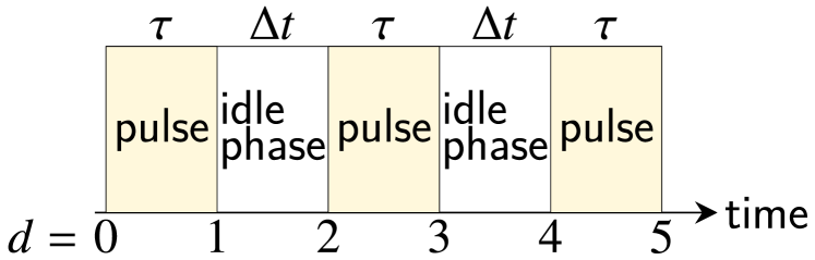
Figure 1: Schematic of the pulse sequence considered in this work. The label $d$ is introduced to indicate the end of each phase ($d=1,\ldots,5$) as well as the initial time ($d=0$).

In order to set the stage for rotations in the presence of environmental degrees of freedom, let us first briefly recall the bare situation. With the Bloch vector of a single qubit

$$\expectationvalue*{\hat{\sigma}_{\alpha}(t)}=\mathrm{tr}\{\hat{\sigma}_{\alpha}\hat{\rho}_{S}(t)\}\,,\ \alpha\in\{x,y,z\}\,,$$ (4)

the qubit’s density operator can be written as $\hat{\rho}_{S}(t)=(\hat{1}+\sum_{\alpha}\expectationvalue*{\hat{\sigma}_{\alpha}(t)}\hat{\sigma}_{\alpha})/2$ with $\hat{1}$ being the identity operator. Thus, a general rotation of the system on the Bloch sphere by an angle $\theta$ around an $\alpha$-axis is given by $\hat{R}_{\alpha}(\theta)=\exp[-i\theta\hat{\sigma}_{\alpha}/2]$. In particular, the time dependence in $\hat{H}_{S}(\Omega,\phi;t)$ can be exactly gauged away via a unitary transformation $\hat{R}_{z}(-\omega_{\mathrm{ex}}t)$ to read

$$\tilde{H}_{S}(\Omega,\phi)=\frac{\hbar(\omega_{q}-\omega_{\mathrm{ex}})}{2}\hat{\sigma}_{z}+\frac{\hbar\Omega}{2}\left(\hat{\sigma}_{x}\cos\phi+\hat{\sigma}_{y}\sin\phi\right)\,.$$ (5)

Accordingly, setting $\omega_{q}=\omega_{\mathrm{ex}}$ implies (cf. Appendix A, Figs. 1, and 2) that, in the rotating frame, rotations $\hat{R}_{x}(\theta)$ are generated by $\tilde{H}(\Omega,0)$ and rotations $\hat{R}_{y}(\theta)$ by $\tilde{H}(\Omega,\pi/2)$. Using the back-transformation $\hat{\rho}_{S}(t)=\hat{R}_{z}(\omega_{q}t)\,\tilde{\rho}_{S}(t)\,\hat{R}_{z}(-\omega_{q}t)$ with the rotating frame density operator $\tilde{\rho}_{S}(t)$, one verifies that in the laboratory frame rotation operations on the qubit correspond one-to-one to the time evolution generated by the Hamiltonian [Eq. (LABEL:eq:H_S)] with a certain choice of parameter values $\Omega$ and $\phi$. The rotation angle $\theta$ is set by $\theta=\Omega\tau$ with the pulse duration $\tau$. In practice, one fixes $\theta$ and $\Omega$ to adjust $\tau$ accordingly.

The common modeling of qubit systems interacting with reservoirs is formulated in the context of open quantum systems. It starts from a system+reservoir Hamiltonian $\hat{H}_{\mathrm{tot}}(\Omega,\phi;t)=\hat{H}_{S}(\Omega,\phi;t)-\hat{V}\hat{X}+\hat{H}_{R}$, where for the sake of simplicity we assume a bilinear coupling between the qubit system with coupling operator $\hat{V}$ and a reservoir $\hat{H}_{R}$ with $\hat{X}$ [30, 31]. In the sequel, we consider two types of errors, namely, bit-flip errors and phase errors, and correspondingly two types of $\hat{V}$. For the bit-flip errors, we adopt the same form as in a previous study [22], which is described as $\hat{V}=\hbar\hat{\sigma}_{x}$. For the phase errors, the operator $\hat{V}$ is set to $\hat{V}=\hbar\hat{\sigma}_{z}$. Note that a different form, $\hat{V}=\hbar\hat{\sigma}_{y}$, is also proposed in previous studies [17, 29].

Now, during the time evolution of the total system in the presence of pulse sequences on the qubit part, the external field with a non-zero amplitude of $\Omega$ rotates the qubit (gate operation) and the time evolution without the external field ($\Omega=0$) between two of these pulse operations, see Fig. 1, is referred to as the “idle phase”. It must be taken into account, for example, considering that there must be synchronizations of qubits during a given multi-qubit protocol. Of course, the state of the isolated qubit in the rotating frame does not change during idle phases. However, for a qubit interacting with reservoirs, decoherence sets in and correlations between qubits and reservoirs evolve such that they are expected to influence the next gate operation. Physically, these latter effects originate from the retarded feedback of the reservoir onto the qubit system which always occurs at sufficiently low temperatures and induces time-nonlocality in the qubit dynamics. Below, we will analyze these effects in more detail. In summary, we vary the amplitude $\Omega$ during a pulse sequence as

$$\left\{\begin{aligned} \Omega\neq&0&&\mbox{(a fixed value during a pulse operation)}\\ \Omega=&0&&\mbox{(during idle phases)}\end{aligned}\right.\,,$$ (6)

with the coupling between the system and reservoir always taken into account. For the sake of simplicity, we model the switching-on and off of the external field as a step function; improvements can be achieved by taking into account the rise time [22, 23].

In order to describe the open dynamics of the qubit during pulse applications of the length $\tau$, we have to take

$$\hat{U}(\Omega,\phi;t,\tau)={\mathcal{T}}\exp[-\frac{i}{\hbar}\int_{t}^{t+\tau}dt^{\prime}\hat{H}_{\mathrm{tot}}(\Omega,\phi;t^{\prime})]$$ (7)

as the rotation operators instead of the bare system generator Eq. (LABEL:eq:H_S). Here, $\mathcal{T}$ is the time-ordering operator. The time evolution of the total density operator is then expressed as

$$\hat{\rho}_{\mathrm{tot}}(\tau+t)= \mathcal{U}_{\mathrm{p}}(\theta,\phi)\hat{\rho}_{\mathrm{tot}}(t)$$ (8)

$$= \hat{U}(\Omega>0,\phi;t,\tau)\,\hat{\rho}_{\mathrm{tot}}(t)\,\hat{U}^{\dagger}(\Omega>0,\phi;t,\tau)$$ (9)

and the reduced density operator of the qubit follows by taking the partial trace over the environmental degrees of freedom, i.e., as $\hat{\rho}_{S}(t)=\mathrm{tr}_{R}\{\hat{\rho}_{\mathrm{tot}}(t)\}$. Above, we have introduced the super-operator for the pulse application $\mathcal{U}_{\mathrm{p}}(\theta,\phi)$ with the relation $\theta=\Omega\tau$. For the idle phase, we define

$$\hat{\rho}_{\mathrm{tot}}(\Delta t+t)= \mathcal{U}_{\mathrm{i}}(\Delta t)\hat{\rho}_{\mathrm{tot}}(t)$$ (11)

$$= \hat{U}(\Omega\!=\!0,\phi;t,\Delta t)\hat{\rho}_{\mathrm{tot}}(t)\hat{U}^{\dagger}(\Omega\!=\!0,\phi;t,\Delta t)\,.$$ (12)

Because the pulse amplitude is zero, an arbitrary phase $\phi$ does not affect the time evolution of the system, and the Hamiltonian is manifestly time-independent.

During the course of this analysis, we also consider impulsive pulses for which we take the limit $\Omega\to\infty$. In this limit, we can ignore the coupling term between the system and reservoir, and the pulse operation is expressed in the following form

$$\hat{\rho}_{\mathrm{tot}}(t)\leftarrow\, \mathcal{U}_{\mathrm{imp}}(\theta,\phi)\hat{\rho}_{\mathrm{tot}}(t)$$ (13)

$$= \hat{R}_{z}(\omega_{q}t)\hat{R}_{\phi}(\theta)\hat{R}_{z}(-\omega_{q}t)$$ (14)

$$\times\hat{\rho}_{\mathrm{tot}}(t)\hat{R}_{z}(\omega_{q}t)\hat{R}_{\phi}(-\theta)\hat{R}_{z}(-\omega_{q}t)\,.$$ (15)

Here, the super-operator $\mathcal{U}_{\mathrm{imp}}(\theta,\phi)$ denotes the application of the impulsive pulse, and we have introduced the operator $\hat{R}_{\phi}(\theta)=\exp\left[-i\theta(\hat{\sigma}_{x}\cos\phi+\hat{\sigma}_{y}\sin\phi)/2\right]$. For more details of the derivation, see Appendix A.

II.2 Exact Time evolution: Extended Hierarchical Equations Of Motion (FP-HEOM)

Reservoirs with a macroscopic number of degrees of freedom are dominantly characterized by Gaussian fluctuations, i.e., by autocorrelation functions $C(t)=\expectationvalue*{\hat{X}(t)\hat{X}(0)}_{R}$ given that $\expectationvalue*{\hat{X}(t)}_{R}=0$ and $\expectationvalue*{\bullet}_{R}=\mathrm{tr}\{\bullet\,\hat{\rho}_{R,eq}\}$ with the equilibrium density operator of the reservoir $\hat{\rho}_{R,eq}=e^{-\beta\hat{H}_{R}}/\mathrm{tr}\{e^{-\beta\hat{H}_{R}}\}$, and $\beta=1/k_{\mathrm{B}}T$. Equivalently, the noise properties of a respective reservoir follow from its spectral noise power

$$S_{\beta}(\omega)=\frac{1}{2\pi}\int_{-\infty}^{+\infty}dtC(t)e^{i\omega t}\,,$$ (16)

where $S_{\beta}(\omega)$ and $S_{\beta}(-\omega)$ are related by the fluctuation-dissipation theorem that can be represented as

$$S_{\beta}(\omega)=\hbar[1+n_{\beta}(\omega)]\,J(\omega)\,.$$ (17)

Here, $n_{\beta}(\omega)=1/[\exp(\beta\hbar\omega)-1]$ is the Bose distribution, and the spectral density $J(\omega)$ is an antisymmetric function with finite bandwidth characterized by a cut-off frequency $\omega_{c}$. Note that this spectral density is directly proportional to the absorptive part of the dynamical susceptibility of the reservoir that can be extracted experimentally. Hence, the spectral noise power serves as the only ingredient required for describing the impact of environmental degrees of freedom on the qubit dynamics. Below, we will discuss in more detail the most relevant noise sources for superconducting qubits and their spectral densities. We already note here though that this modeling is not only limited to reservoirs with underlying bosonic degrees of freedom but, effectively, may also apply, for example, to low energy excitations of quasiparticles around Fermi surfaces.

Studying the open quantum dynamics according to the above pulse protocol is a highly non-trivial task since the combined time evolution is not separable. Standard procedures are then second-order perturbative approaches based on the Born–Markov approximation, including the Bloch–Redfield and the Lindblad equation, respectively. However, these approaches turn out to be insufficient in light of the growing accuracy, and in turn sensitivity, of actual qubit devices. For example, it was suggested that a more elaborate method beyond the Born–Markov approximation is needed when we consider dephasing dynamics with $1/f$ noise [32]. In addition, it was reported that the Born approximation causes errors for simulations with multiple pulses [33, 34] and that it provides inaccurate predictions for ground-state populations after a reset via equilibration [22].

Hence, in order to conduct numerical simulations in a rigorous manner valid in all ranges of parameter space and applicable to a broad class of reservoirs, we adopt the hierarchical equations of motion (HEOM). Its derivation starts from the formally exact Feynman–Vernon path integral representation of the reduced density operator (RDO) of the system, where the impact of the reservoir is completely determined by the correlation $C(t)$. The corresponding reduced quantum dynamics can exactly be mapped onto a nested hierarchy of equations of motion for auxiliary density operators (ADOs). As we have shown recently [28], the key ingredient is the barycentric representation of $S_{\beta}(\omega)$ which provides, to any given accuracy, a representation of the form

$$C(t)=\sum_{k=1}^{K}d_{k}e^{-i\omega_{k}t-\gamma_{k}t}\qquad(t>0)$$ (18)

with a minimal number $K$ of effective reservoir modes. These are characterized by frequencies $\omega_{k}$, damping rates $\gamma_{k}>0$, and complex-valued amplitudes $d_{k}=d^{\prime}_{k}+id^{\prime\prime}_{k}$. Thus, the correlation $C(t)$ is described by a set of a moderate number of damped harmonic modes even at zero temperature and also for structured reservoir densities. While the conventional HEOM was limited to higher temperatures and smooth reservoir spectral densities, the representation Eq. (18) turns it into an extremely efficient simulation tool of general applicability.

We here display the structure of this new Free-Pole HEOM (FP-HEOM) only and refer to Appendix B.1 for more details. The dynamics of the ADOs follow from

$$\frac{\partial\hat{\rho}_{\vec{m},\vec{n}}}{\partial t}= -i\mathcal{L}_{S}\hat{\rho}_{\vec{m},\vec{n}}-\sum_{k=1}^{K}(m_{k}z_{k}+n_{k}z_{k}^{*})\hat{\rho}_{\vec{m},\vec{n}}$$ (19)

$$-i\sum_{k=1}^{K}\mathcal{L}_{k}^{+}\hat{\rho}_{\vec{m},\vec{n}}-i\sum_{k=1}^{K}\mathcal{L}_{k}^{-}\hat{\rho}_{\vec{m},\vec{n}}$$ (20)

with multi-index $(\vec{m},\vec{n})\equiv\{m_{1},\ldots,m_{K},n_{1},\ldots,n_{K}\}$ associated with forward and backward system path in the original path integral, complex-valued coefficients $z_{k}\equiv\gamma_{k}+i\omega_{k}$ according to Eq. (18), and raising and lowering super-operators $\mathcal{L}_{k}^{+}$ and $\mathcal{L}_{k}^{-}$, acting on the $k$th quasimode and involving $\hat{V}$. It can be shown that, in fact, this equation is the Fock state representation in an extended Hilbert space including the qubit as well as the quasimodes [35].

To obtain a closed set of equations for numerical calculations, Eq. (20) is truncated by defining the depth of the hierarchy as $\mathcal{N}=\sum_{k=1}^{K}(m_{k}+n_{k})$, and always set $\hat{\rho}_{\vec{m},\vec{n}}(t)=0$ for the ADOs with $\mathcal{N}>\mathcal{N}_{\max}$. We set $\mathcal{N}_{\max}$ to a sufficiently large integer to obtain converged results. The physical RDO of the qubit system appears as $\hat{\rho}_{S}(t)=\mathrm{tr}_{R}\{\hat{\rho}_{\mathrm{tot}}(t)\}=\hat{\rho}_{\vec{0},\vec{0}}(t)$. When the system Hamiltonian and the system operator in the system–reservoir interaction commute, i.e., $[\hat{H}_{S}(\Omega,\phi;t),\hat{V}]=0$, we can rigorously express the RDO without the ADOs. This is the case for $\Omega=0$ and $\hat{V}=\hbar\hat{\sigma}_{z}$.

III Preliminaries: Spectral densities and parameters

In this section, we specify a class of spectral densities relevant for superconducting qubit platforms, particularly of the transmon type. We note that a substantial number of studies [36, 20, 32, 18] have provided a quite accurate picture of relevant noise sources on a broad range of timescales from intrinsic qubit timescales of nanoseconds to macroscopic scales of hours for rare events. Here, we are interested in decoherence processes on frequency scales from GHz down to the range of MHz or kHz. On these scales three dominant noise sources have been identified:

1. Electromagnetic fields: Fluctuations of electromagnetic modes are typically modeled according to an Ohmic reservoir (Ohmic resistor) with $J_{\mathrm{em}}(\omega)\sim\omega$ up to some cutoff frequency $\omega_{c}$ [31, 37, 38].

2. Two level fluctuators (TLFs): It has been suggested that transmon qubits are affected by $1/f^{\varepsilon}$ ($\varepsilon>0$) noise in the low-frequency region $f\ll 1$ [32, 36], and it was reported that two level fluctuators (random telegraph noise) in the circuits work as a source of this noise [39, 31, 40, 41].

3. Quasiparticles: Residual quasiparticles in superconductors have detrimental effects on the qubit performance; under some approximations the spectral noise power of quasiparticle noise has been shown to be of the form $S_{\beta,\mathrm{qp}}(\omega)\sim 1/\sqrt{\omega}$ at low temperatures [42].

These major types of noise can be captured by the following class of spectral densities

$$J_{s}(\omega)=\mathrm{sgn}(\omega)\frac{\kappa\omega_{\mathrm{ph}}^{1-s}|\omega|^{s}}{\left(1+(\omega/\omega_{c})^{2}\right)^{2}}$$ (21)

parameterized by a spectral exponent $s$. Here, $\kappa$ is the coupling rate between the system and reservoir, and $\omega_{c}$ a cutoff frequency. The frequency $\omega_{\mathrm{ph}}$ is usually introduced to fix the unit of $\kappa$ irrespective of the exponent $s$; here we put $\omega_{\mathrm{ph}}=\omega_{q}$ so that $J_{s}(\omega_{q})$ takes the same value regardless of $s$. The sign function $\mathrm{sgn}(\omega)$ guarantees the property $J_{s}(-\omega)=-J_{s}(\omega)$. For convenience and following a previous study [22], the cutoff function is chosen to be $1/(1+(\omega/\omega_{c})^{2})^{2}$, where the dependence of explicit results on this specific form is negligible as long as $\omega_{c}\gg\omega_{q}$ [31].

The above class of spectral densities includes the Ohmic case ($s=1$) as well as sub- ($0<s<1$) and super-Ohmic ($s>1$) baths, respectively. More specifically, in the low-frequency range the corresponding spectral noise power [Eq. (17)] saturates to a finite value in the Ohmic case (i), i.e., $S_{\beta,s=1}(\omega=0)=\kappa k_{\mathrm{B}}T$, while in the sub-Ohmic case it scales according to

$$S_{\beta,s<1}(\omega\to 0)\simeq\kappa k_{\mathrm{B}}T(\omega_{q}/\omega)^{1-s}\,.$$ (22)

With the relation $\varepsilon=1-s$, this spectral noise power exhibits $1/f^{\varepsilon}$-like behavior (ii), and it captures quasiparticle noise (iii) for $s=1/2$. It is worth noting that for the TLF-noise (ii), the linear dependence on the temperature in Eq. (22) corresponds to previous studies [43, 44], while a $T^{2}$-dependence has also been reported  [45, 46].

In this study, we particularly investigate how the qubit dynamics changes with respect to the spectral exponent $s$, by considering values $s=1,1/2,1/4,1/8$ and $1/14$. Further, we set $\omega_{q}$ as the unit of frequency and fix parameter values to low temperatures $\beta\hbar\omega_{q}=5$, high cut-off frequency $\omega_{c}/\omega_{q}=50$, and weak coupling to the reservoir $2\pi\hbar\kappa=0.04$. For example, at a reservoir temperature of $T=30$mK, this corresponds to $\omega_{q}\approx 2\pi\times 3.1$GHz. Pulse amplitudes $\Omega$ (pulse durations $\tau$ accordingly) and durations of the idle phase $\Delta t$ are tuned over a wide range of parameters.

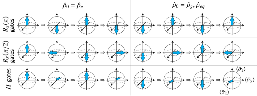
Figure 2: Schematics of time evolution of ideal Bloch vectors in the rotating frame. The right arrows ($\Rightarrow$) indicate the pulse applications. Note that in the case $\hat{\rho}_{eq}$, the length of the Bloch vector is smaller than $1$, while the direction of the vector is same as the direction in the case $\hat{\rho}_{g}$.

IV Sequences of gate operations

In this section, we analyze the performance of a single qubit subject to sequences of gate operations in the presence of noise sources according to Eq. (21). We emphasize that the numerical simulations based on the FP-HEOM [Eq. (20)] provide highly accurate data including the full non-Markovianity. By sweeping parameters over a wide range of values we obtain a comprehensive picture of the qubit performance and the relevance of qubit–environmental correlations.

More specifically, we consider pulse sequences that consist of three gate operations separated by two idle phases, see Fig. 1. For the gate operations our focus lies on three types of operations, namely, (i) rotations with angle $\pi$ about the $x$ axis, denoted $R_{x}(\pi)$, (ii) rotations with angle $\pi/2$ about the $x$ axis, denoted $R_{x}(\pi/2)$, and (iii) a Hadamard gate, denoted $H$. The duration of the three pulses $\tau$ is set equal during the sequence as well as the time span $\Delta t$ for the two idle phases. Each sequence of gate operations is then described by a set of gate-specific super-operators $\mathcal{U}_{\mathrm{p}}(\theta,\phi)$ while during the idle phases the time evolution is generated by $\mathcal{U}_{\mathrm{i}}(\Delta t)$.

Numerically, we practice the following procedure: For the first pulse application, the time evolution is calculated for a fixed value $\phi$ up to the pulse duration $\tau=\theta/\Omega$. This is followed by the time evolution under the condition $\Omega=0$ up to $\Delta t$ for the first idle phase. We repeat these calculations for the subsequent pulses/idle phases. In the situation of impulsive pulses, $\mathcal{U}_{\mathrm{p}}(\theta,\phi)$ is replaced by $\mathcal{U}_{\mathrm{imp}}(\theta,\phi)$, and this super-operator is applied to all RDOs and ADOs, where the latter implies the replacement $\hat{\rho}_{\mathrm{tot}}(t)\to\hat{\rho}_{\vec{m},\vec{n}}(t)$ in Eq. (15). Note that we treat the open quantum dynamics over the full sequence such that the RDO and ADOs obtained at the end of a previous phase are used as the initial states for the subsequent ones.

For the initial states prior to the first gate operation, we consider three initial states: (a) the qubit is in the excited state, $\hat{\rho}_{\vec{0},\vec{0}}(0)=\outerproduct{1}{1}$ and $\hat{\rho}_{\vec{m}\neq\vec{0},\vec{n}\neq\vec{0}}(0)=0$, (b) the qubit is in the ground state, $\hat{\rho}_{\vec{0},\vec{0}}(0)=\outerproduct{0}{0}$ and $\hat{\rho}_{\vec{m}\neq\vec{0},\vec{n}\neq\vec{0}}(0)=0$, and (c) the qubit resides in the equilibrium state of the total Hamiltonian. Here, we have introduced the ket-vector of the ground (excited) state of the system as $\ket{0}$ ($\ket{1}$). The initial states (a) and (b) correspond to factorized states $\outerproduct{1}{1}\otimes\hat{\rho}_{R,eq}$ and $\outerproduct{0}{0}\otimes\hat{\rho}_{R,eq}$, respectively. For the case (c), before the pulse applications, the relaxation dynamics of the qubit without the external field ($\Omega=0$) starting from $\outerproduct{1}{1}\otimes\hat{\rho}_{R,eq}$ is evaluated until a steady state is reached. Since the system reaches the same steady state irrespective of the initial state, we identify this steady state with the correlated thermal equilibrium state of the total compound, i.e., $\hat{\rho}^{\mathrm{c}}_{S,eq}=\mathrm{tr}_{R}\{e^{-\beta\hat{H}_{\mathrm{tot}}(\Omega=0,\phi;t)}\}/\mathrm{tr}\{e^{-\beta\hat{H}_{\mathrm{tot}}(\Omega=0,\phi;t)}\}$ [47]. For more details of the preliminary equilibration process, see Appendix D.1.1. In short, we denote these three types of initial states as (a) $\hat{\rho}_{0}=\hat{\rho}_{e}$, (b) $\hat{\rho}_{g}$ and (c) $\hat{\rho}_{eq}$, respectively.

From the perspective of experimental implementations, we assume that the qubit prior to the gate sequence is equilibrated with respect to the total Hamiltonian. In the domain, where superconducting qubits are operated and at weak couplings to the environment, this implies basically only weak qubit–reservoir correlations in thermal equilibrium. An initialization pulse can then be assumed to prepare the compound into either (a) $\outerproduct{1}{1}\otimes\hat{\rho}_{R,eq}$ or (b) $\outerproduct{0}{0}\otimes\hat{\rho}_{R,eq}$ with equilibrium correlations between the qubit and reservoir basically destroyed. For case (c), we simply use the total equilibrium state as the initial state, and no initialization pulse is required; the qubit resides almost exclusively in its ground state correlated with the reservoir (when projecting $\hat{\rho}^{\mathrm{c}}_{S,eq}$ onto $\outerproduct{0}{0}$).

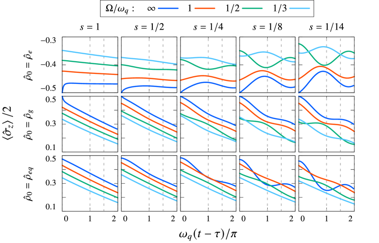
Figure 3: Dynamics of the expectation value $\expectationvalue*{\hat{\sigma}_{z}(t)}/2$ during the first idle phase with various initial states $\hat{\rho}_{0}$ and spectral exponents $s$. The sequence of $R_{x}(\pi)$ gates is considered. The gray vertical dashed lines indicate the time duration $\Delta t\omega_{q}/\pi=0,1,3/2,2$, respectively, which corresponds to the time $d=2$ in Fig. 1.

To illustrate the described protocol, we show in Fig. 2 a cartoon displaying the status of the qubit’s Bloch vector in the rotating frame after the application of the respective gate operation starting from a specific initial state. The dynamics during the idle phases which appear between the second and the third and the third and the fourth snapshot is not shown, since the system in the rotating frame ideally remains in a certain state during an idle phase.

The Bloch vector in the rotating frame is defined as

$$\expectationvalue*{\tilde{\sigma}_{\alpha}(t)}=\mathrm{tr}\{\hat{\sigma}_{\alpha}\hat{R}_{z}(-\omega_{q}t)\hat{\rho}_{S}(t)\hat{R}_{z}(\omega_{q}t)\}\,$$ (23)

with the reduced density operator $\hat{\rho}_{S}(t)$.

In order to quantify the (detrimental) impact of reservoirs onto the performance of the qubit under the gate operations, we introduce the fidelity

$$F(t)=\left(\mathrm{tr}\left\{\sqrt{\sqrt{\hat{\rho}_{\mathrm{iso}}(t)}\hat{\rho}_{S}(t)\sqrt{\hat{\rho}_{\mathrm{iso}}(t)}}\right\}\right)^{2}\,.$$ (24)

Here the density operator for the isolated qubit system is introduced as $\hat{\rho}_{\mathrm{iso}}(t)$. For its evaluation identical pulse sequences compared to the dissipative case are considered with the only difference that we set $\hat{V}=0$ with initial states $\hat{\rho}_{\mathrm{iso}}(0)=\outerproduct{1}{1}$, $\outerproduct{0}{0}$ and $\hat{\rho}^{\mathrm{c}}_{S,eq}$ respectively.

IV.1 $R_{x}(\pi)$ gates

Expressed in terms of the super-operator introduced in Eqs. (LABEL:eq:Upulse)–(15), the sequence of three $R_{x}(\pi)$ gates is described by the evolution

$$\mathcal{U}_{\mathrm{p}}(\pi,0)\mathcal{U}_{\mathrm{i}}(\Delta t)\mathcal{U}_{\mathrm{p}}(\pi,0)\mathcal{U}_{\mathrm{i}}(\Delta t)\mathcal{U}_{\mathrm{p}}(\pi,0)\,.$$ (25)

We start by discussing typical dynamical features that reveal interesting physics and have direct impact on the fidelities to be analyzed below. By way of example, we depict in Fig. 3 snapshots of the qubit dynamics during the first idle phase (segment $1<d\leq 2$ in Fig. 1) for various driving amplitudes $\Omega$, i.e., pulse durations $\tau=\pi/\Omega$, and spectral exponents $s$. Clearly, for $\tau=0$, the qubit starts after the impulsive $\pi$-pulse in the ideally rotated state with $\expectationvalue*{\hat{\sigma}_{z}}/2=\pm 0.5$ (for ground/excited state initial preparation). It then tends to relax monotonously for reservoirs with $s>1/2$ with the initial states $\hat{\rho}_{0}=\hat{\rho}_{g}$ and $\hat{\rho}_{eq}$, while for smaller spectral exponents (towards $1/f$-noise) an oscillatory behavior sets in due to the stronger portion of low frequency modes which induce a sluggish dynamics and strongly retarded feedback of the reservoir. For finite duration of the first gate pulse (finite $\Omega$, $\tau>0$), the qubit starts progressively further away from its ideal value since relaxation happens to occur already during the gate pulse and pursues in the subsequent idle phase. In relative terms, this process is more pronounced when starting initially from an excited state compared to a ground state preparation. Interestingly, deeper into the sub-Ohmic domain, $s\leq 1/8$, and with increasing duration $\Delta t$ of the idle phase [larger $\omega_{q}(t-\tau)/\pi$ in Fig. 3], the qubit dynamics for different $\tau$ interchange: less ideal $\expectationvalue*{\hat{\sigma}_{z}}$-values at the beginning of the idle phase are overcompensated by an oscillatory reservoir-induced dynamics such as to exceed those with more ideal starting values. This ‘switching’ may lead to a somewhat counter-intuitive behavior of respective fidelities as we will see now.

Figures 4(a)–4(c) display heatmaps of fidelities for the three respective initial states. For each initial preparation, the fidelity at the end of each of the five segments ($d=1,\ldots 5$) in Fig. 1 is depicted for various values of the spectral exponent $s$, from an Ohmic noise source ($s=1$) to a reservoir with deep sub-Ohmic fluctuations ($1/f$-noise). Each pair $(d,s)$ defines a super-cell consisting of $4\times 4$ cells, for which the driving amplitude $\Omega$ and the duration of the idle phase $\Delta t$ are varied, see Fig. 4(d).

Before we come to the details, we summarize the overall picture: The tendency towards lower fidelities can be seen (i) for weaker drive amplitudes (i.e., longer gate pulse durations), (ii) for longer idle times (with some exceptions, see below), and (iii) when starting from the excited state. The overall dependence on the spectral exponent $s$ (type of noise) is weak for the $R_{x}(\pi)$ gate. In general, fidelities in case (c) are higher than those in case (b), although the initial states $\hat{\rho}_{g}$ and $\hat{\rho}_{eq}$ are close to each other, and the dynamics are similar (the middle and bottom panels of Fig. 3). This is mainly due to the difference of the reference density operator $\hat{\rho}_{\mathrm{iso}}(t)$; $\hat{\rho}_{\mathrm{iso}}(0)=\outerproduct{0}{0}$ in case (b) and $\hat{\rho}_{\mathrm{iso}}(0)=\hat{\rho}^{\mathrm{c}}_{S,eq}$ in case (c). However, this picture is blurred as some counter-intuitive features appear.

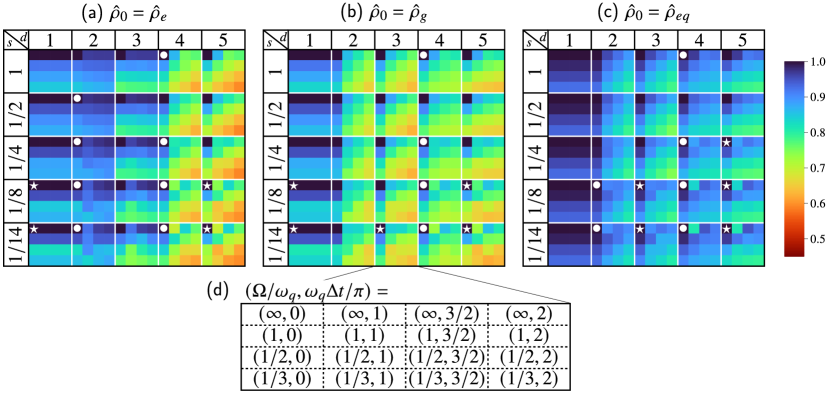
Figure 4: (a)–(c) Heatmaps of the fidelity of the $R_{x}(\pi)$ gates measured at the end of each phase, $d$, with various spectral exponents, $s$. The initial states are given by (a) $\hat{\rho}_{e}$, (b) $\hat{\rho}_{g}$, and (c) $\hat{\rho}_{eq}$, respectively. The whole heatmap is divided into $5\times 5$ supercells, and a supercell consists of $4\times 4$ cells. For each supercell, the values of $\Omega$ and $\Delta t$ are varied, while $d$ and $s$ are fixed. The circle and star symbols in the upper-left corner of the supercell indicate the violation of the expected order: see the main text for the definition of the expected order. (d) Legend for the supercell.

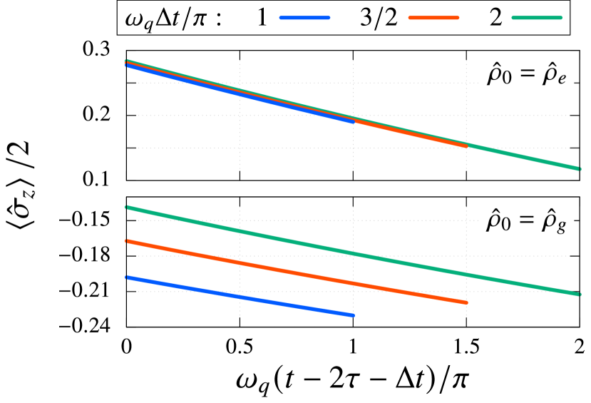
Figure 5: Dynamics of the expectation value $\expectationvalue*{\hat{\sigma}_{z}(t)}/2$ during the second idle phase for the Ohmic reservoir ($s=1$) with the pulse duration $\Omega/\omega_{q}=1/3$. The initial and terminal point of each curve correspond to the time $d=3$ and $4$, respectively.

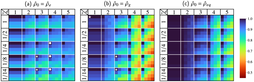
Figure 6: Heatmaps of the fidelity of the $R_{x}(\pi/2)$ gates measured at the end of each phase, $d$, with various spectral exponents, $s$. The initial states are given by (a) $\hat{\rho}_{e}$, (b) $\hat{\rho}_{g}$, and (c) $\hat{\rho}_{eq}$, respectively. The parameter values of each cell are the same as Fig. 4. The circle and star symbols in the upper-left corner of the supercell indicate the violation of the expected order, in the same way as Fig. 4.

This brings us to a more detailed discussion: We first mention that at low temperatures, relaxation occurs pre-dominantly from an excited state toward the ground state. Hence, the expectation is that whenever the qubit, after a gate pulse, is ideally positioned in the excited state, the fidelity at the end of an idle phase is smaller compared to the situation when it is supposed to be in the ground state. This is confirmed by comparing columns $d=2$ in Figs. 4(a) and 4(b). One also observes that with increasing duration of the idle phase for $d=2$ in case (a) the fidelity generally increases while it decreases with growing $\Delta t$ for $d=2$ in case (b). Note that the former tendency is opposed to the general tendency (ii), i.e., this is the exceptional case mentioned above.

To analyze the tendency at $d=4$, we display typical dynamics during the second idle phase in Fig. 5. Comparing the fidelities at $d=3$ and $4$ for each gate sequence, which correspond to the initial and terminal point of each curve in Fig. 5, respectively, one expects qualitatively an opposite behavior from cases at $d=2$: loss of the fidelity in case (a) (because the gate has positioned the qubit close to its excited state) and partial recovery of the fidelity in case (b) (when the second gate has positioned it back into the ground state). This is indeed the case and leads to relatively larger fidelities at the end of the sequence ($d=5$) in case (b) compared to case (a). In terms of the duration $\Delta t$, the fidelity at $d=4$ is expected to shrink in both cases as $\Delta t$ grows: The relaxation behavior directly results in this expectation in case (a). Although the partial recovery occurs in case (b), the initial difference in Fig. 5 with respect to $\Delta t$ is too large to be compensated. In case (c), the same expectation as in case (b) holds.

However, there are deviations from this behavior. They are indicated by the circle symbols in Figs. 4(a)–4(c) and are due to the following two factors: (i) Instantaneous gate pulses ($\tau=\pi/\Omega=0$): In this situation, drastic changes of the qubit–reservoir correlations emerge during the idle phase and non-monotonous behavior in the qubit populations is observed (blue curves in Fig. 3). Note in passing that the fidelities for $\tau=\Delta t=0$ are always $1$ because no relaxation and decoherence occur in this case. (ii) Long-range qubit–reservoir correlations (memory effects): Since the duration of idle phases is much shorter than equilibration times of the qubit, non-equilibrium dynamics appear throughout the complete sequence. This implies that retardation effects induce correlations between the dynamics in subsequent idle phases ($1<d\leq 2$ and $3<d\leq 4$) as well as between idle phases and gate segments. These memory effects influence the fidelities as well and, as detailed inspection reveals, lead in some cases to deviations from the general picture described above. For example, in the deep sub-Ohmic regime ($s=1/8,1/14$), the qubit and reservoir can coherently interact with each other multiple times (for more details, see Appendix C). This non-Markovian effect induces oscillations in the populations (Fig. 3) and a non-monotonous trend in the fidelities when sweeping pulse and idle-phase parameters. We emphasize that within the Born–Markov approximation the reservoir is treated such that it were always in the bare equilibrium state $\hat{\rho}_{R,eq}$ and non-monotonous phenomena (i) and (ii) are not predicted within the framework of Bloch–Redfield and Lindblad simulations.

There is another very interesting observation that we stress here. One expects that for longer gate pulses the fidelity deteriorates due to a longer interaction time between the system and reservoir. We have confirmed this tendency within the frame of Lindblad equations (results are not shown). This implies that in Figs. 4(a)–4(c) the fidelity aligns in descending order from top to bottom at $d=1,3$, and $5$. The star symbols indicate the violation of this expectation. The reason for this deviation is the following: Both, the angle between the experimentally obtained and the ideal Bloch vectors, as well as the length of the Bloch vector contribute to the fidelity. As depicted in Appendix D.1.2, the bare qubit frequency $\omega_{q}$ (no reservoir) differs from the effective qubit frequency (in the presence of a reservoir). If the frequency of the external pulse is misaligned with the effective qubit frequency, the rotation axis changes from the desired one, and the fidelity deteriorates at the end of the pulse application, $\tau=\theta/\Omega$. Furthermore, the effective qubit frequency varies in time so that the pattern of the fidelity may not be intuitive.

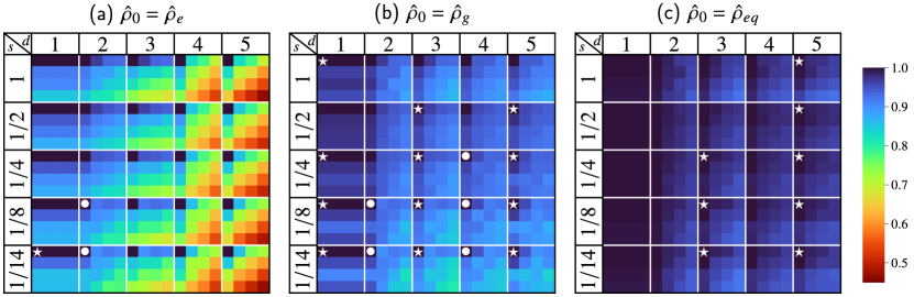
Figure 7: Heatmaps of the fidelity of the Hadamard ($H$) gates measured at the end of each phase $d$, with various spectral exponents $s$. The initial states are given by (a) $\hat{\rho}_{e}$, (b) $\hat{\rho}_{g}$, and (c) $\hat{\rho}_{eq}$, respectively. The parameter values of each cell are the same as Fig. 4. The circle and star symbols in the upper-left corner of the supercell indicate the violation of the expected order, in the same way as Fig. 4.

IV.2 $R_{x}(\pi/2)$ gates

Let us now turn to the $R_{x}(\pi/2)$ gate which follows from the following sequences [cf. Eqs. (LABEL:eq:Upulse)–(15)]

$$\mathcal{U}_{\mathrm{p}}\left(\frac{\pi}{2},0\right)\mathcal{U}_{\mathrm{i}}(\Delta t)\mathcal{U}_{\mathrm{p}}\left(\frac{\pi}{2},0\right)\mathcal{U}_{\mathrm{i}}(\Delta t)\mathcal{U}_{\mathrm{p}}\left(\frac{\pi}{2},0\right)\,.$$ (26)

The qubit dynamics during the first idle phase can be seen in Fig. 17 in Appendix E.1. They reveal again Markovian and non-Markovian behavior depending on the spectral exponents. Corresponding fidelities are seen in Fig. 6 with the same structuring and the same value of the parameters as above for the $\pi$-gate. However, the pulse duration is only half of that for the $\pi$-gate, of course, given by $\tau=\pi/(2\Omega)$.

The final fidelity is the largest for the initialization (a). As discussed in Sec. IV.1, this is because at the beginning of the second idle phase, the desired state of the qubit is the ground state $\outerproduct{0}{0}$ (Fig. 2), and the relaxation process constructively supports this state. The cause of the difference of the fidelity between the cases (b) and (c) is mainly the difference of the reference state, which is the same as in the case of the $R_{x}(\pi)$ sequence. With a fixed $d$, $\Omega$ and $\Delta t$, the fidelity in general tends to take a maximum value for medium sub-Ohmic reservoirs with $s=1/2$ and $1/4$ while minimum values appear for exponents $s=1$ (Ohmic) and $1/14$ (deep sub-Ohmic), i.e., reservoirs with intermediate exponents have the least detrimental impact on fidelities for $R_{x}(\pi/2)$ gates.

Comparing the supercells of initial preparations $\hat{\rho}_{e}$ and $\hat{\rho}_{g}$ in column $d=1$, we find that the fidelity of the latter exceeds that of the former. As depicted in Fig. 2, the first pulse application corresponds in the rotating frame to the rotation of the Bloch vector from $(0,0,1)$ to $(0,-1,0)$ in case (a), and from $(0,0,-1)$ to $(0,1,0)$ in case (b). The positive $\expectationvalue*{\hat{\sigma}_{z}(t)}$ (excited state) is converted to a superposition (coherence) via the $\pi/2$-pulse in case (a), while the negative $\expectationvalue*{\hat{\sigma}_{z}(t)}$ (ground state) contributes in case (b): In any case, larger absolute values, $|\expectationvalue*{\hat{\sigma}_{z}(t)}|$, result in larger fidelities after the pulse application. Because decay of $|\expectationvalue*{\hat{\sigma}_{z}(t)}|$ is more pronounced in the excited state, a superposition with a lower fidelity is created in case (a). This in turn suggests creation of superposition states with higher fidelities starting initially from a ground state.

Similarly to the $R_{x}(\pi)$ gates, we expect the following tendency of the fidelity in each supercell: In descending order from top to bottom in $d=1,3$ and $5$, and from left to right in $d=2$ and $4$, respectively. In the case of the $R_{x}(\pi/2)$ gates, however, we cannot observe the violation of this expected order in $d=2$ [as is the case for the $R_{x}(\pi)$ gate]. Namely, during the first idle phase, the $\expectationvalue*{\tilde{\sigma}_{y}}$ element of the Bloch vector mainly contributes to the fidelity. Because the reservoir affects the fidelity during this phase through the decoherence process rather than the population-relaxation process, the tendency of the order is different compared to the $R_{x}(\pi)$ gates. As depicted in Appendix E.1, the peculiar behavior for $\Omega=\infty$ or small $s$ found in the $R_{x}(\pi)$ sequences is not observed here, or rather, the expected order is obtained. In $d=4$, the fidelity is again determined mainly by $\expectationvalue*{\hat{\sigma}_{z}}$, and the oscillatory pattern of the populations again contributes to the development of the fidelities. Similarly to the $R_{x}(\pi)$ gates (Fig. 3 and Sec. IV.1), the intra-segment oscillations change the order for lower $s$ when the qubit state is close to the ground state, which is found in case (a) for reservoirs with $s=1/4,1/8$ and $1/14$.

Overall, a violation of the expected order during the pulse application ($d=1$, $3$, and $5$) is observed only in a smaller number of supercells compared to the case of $R_{x}(\pi)$ gates. The differences between initial and final states (Fig. 2), and the length of the pulse duration may be responsible for this different behavior.

IV.3 Hadamard ($H$) gates

The third gate sequence that we analyze here, consists of three Hadamard gates according to Eqs. (LABEL:eq:Upulse)–(15)

$$\mathcal{U}_{\mathrm{p}}\left(\frac{\pi}{2},-\frac{\pi}{2}\right)\mathcal{U}_{\mathrm{i}}(\Delta t)\mathcal{U}_{\mathrm{p}}\left(\frac{\pi}{2},\frac{\pi}{2}\right)\mathcal{U}_{\mathrm{i}}(\Delta t)\mathcal{U}_{\mathrm{p}}\left(\frac{\pi}{2},-\frac{\pi}{2}\right)\,.$$ (27)

Note that the virtual $Z$ gate [48] is considered here. In Fig. 7, we depict corresponding heatmaps of the fidelity, where the parameter values $s$, $d$, $\Omega$ and $\Delta t$ for each cell are the same as in Fig. 4 while the pulse duration is the same as the one in Fig. 6.

Overall, the fidelity is maximum in the case of an equilibrium initial preparation $\hat{\rho}_{eq}$, while it takes minimum values for the qubit being initially in an excited state $\hat{\rho}_{e}$: The value $F(t)=0.467$ for Ohmic reservoirs ($s=1$) in $d=5$ with $\Omega/\omega_{q}=1/3$ and $\omega_{q}\Delta t/\pi=2$ is the worst for all the cells in Figs. 4, 6, and 7. This is mainly due to two factors, namely, the first pulse application ($0<d\leq 1$) and the second idle phase ($3<d\leq 4$). As discussed in Sec. IV.2, the rotation with an angle $\pi/2$ starting from the excited state is most subject to noise. This tendency was found to be independent of the rotational axis. In addition, at the beginning of the second idle phase the qubit ideally starts again from an excited state when it was prepared there before the first gate pulse. Since the relaxation process causes more detrimental effects on the excited state than on the ground state, as discussed in Sec IV.1, these two contributions add up to reduce the fidelity substantially.

The reason for the better performance starting from an initial state $\hat{\rho}_{eq}$ compared to that for $\hat{\rho}_{g}$ is the same as above for the $R_{x}(\pi)$ and $R_{x}(\pi/2)$ gates. In terms of the reservoir exponent $s$, it is true also for $H$ gates that the fidelity for $s=1/2$ and $1/4$ is maximum while that with $s=1$ and $1/14$ is minimum for fixed $d$, $\Omega$ and $\Delta t$. In fact, this tendency is here even more significant than in the case of $R_{x}(\pi/2)$ gates.

It is worth noting that at $d=2$, a violation of the expected order for the fidelity is observed in the deep sub-Ohmic domain $s=1/8$ and $1/14$ for initial states $\hat{\rho}_{e}$ and $\hat{\rho}_{g}$. Here, the expected order is defined in the same way as in Sec. IV.2. As depicted in Appendix E.2, a significant decoherence that is not observed in the $R_{x}(\pi/2)$ gates contributes to this violation. Namely, the different rotational axis leads to significantly different behavior during the first idle phase. During the second idle phase starting with $\hat{\rho}_{g}$, the qubit is close to the ground state. This situation is similar to that in Fig. 6(a) at $d=4$: Again the strongly non-Markovian behavior corresponding to oscillatory qubit dynamics for $s\leq 1/4$ induces a violation of the expected order, see Fig. 7(b) [cf. with Fig. 6(a)].

As for the pulse-application phase, a violation is observed in different cells in Fig. 7 compared to Fig 6. The static phase of the external field $\phi$ induces differences in the appearance, as gate operations $\hat{R}_{x}(\pi/2)$ are used in Fig. 6 while $\hat{R}_{y}(\pm\pi/2)$ in Fig. 7.

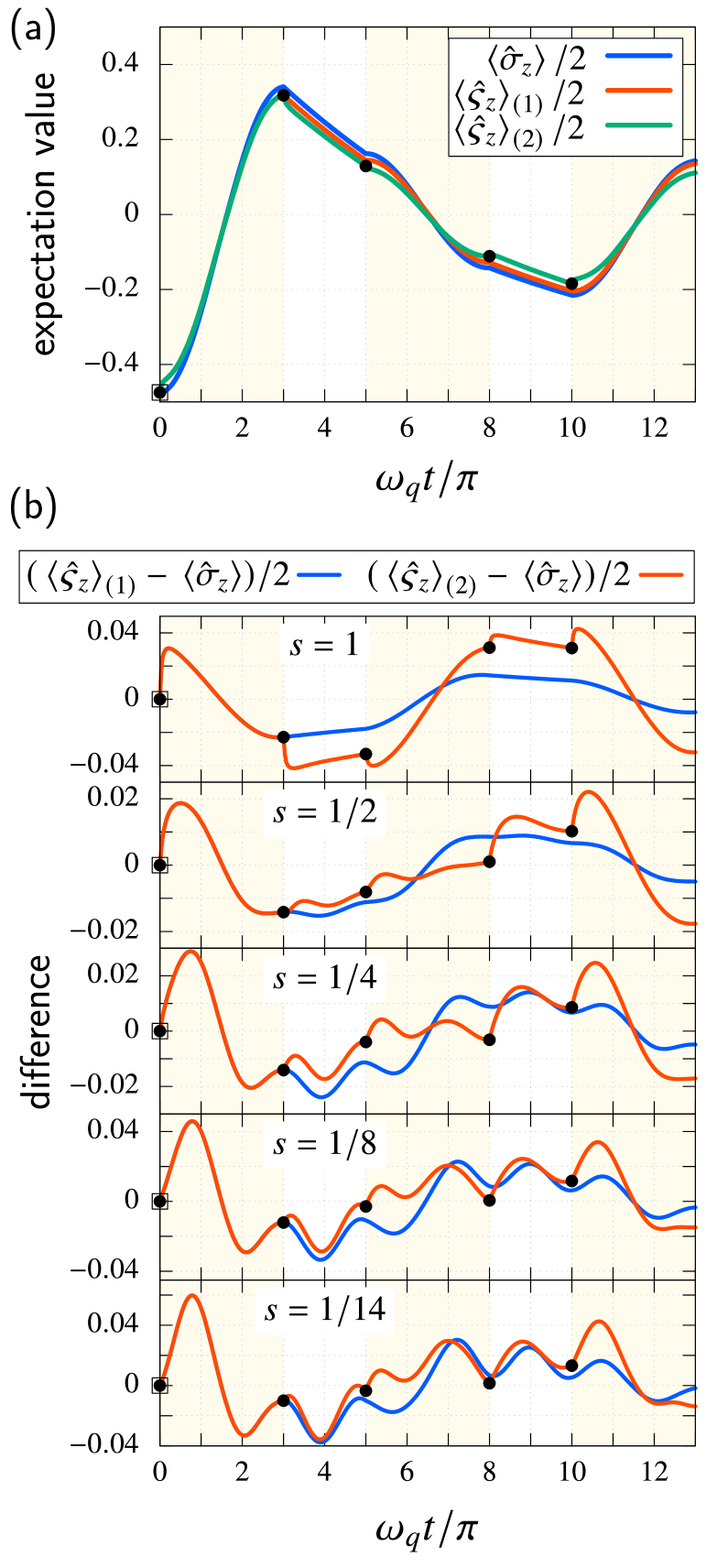
Figure 8: (a) Whole dynamics of the expectation value $\expectationvalue*{\hat{\sigma}_{z}(t)}/2$, $\expectationvalue*{\hat{\varsigma}_{z}(t)}_{(1)}/2$, and $\expectationvalue*{\hat{\varsigma}_{z}(t)}_{(2)}/2$ with the $R_{x}(\pi)$ sequence. The initial state is given by $\hat{\rho}_{0}=\hat{\rho}_{eq}$, and $\Omega/\omega_{q}$ and $\omega_{q}\Delta t/\pi$ are set to $1/3$ and $2$, respectively. The shaded areas indicate the pulse-application phase, which corresponds to the schematic of Fig. 1. We applied the projection operator $\mathcal{P}[\hat{\rho}_{\mathrm{tot}}(t)]=\mathrm{tr}_{R}\{\hat{\rho}_{\mathrm{tot}}(t)\}\otimes\hat{\rho}_{R,eq}$ at times indicated by the empty squares [at $t=0$, $\expectationvalue*{\hat{\varsigma}_{z}(t)}_{(1)}$] and filled circles [$\expectationvalue*{\hat{\varsigma}_{z}(t)}_{(2)}$]. The dynamics without the projection operators $\expectationvalue*{\hat{\sigma}_{z}(t)}$ are also depicted as a reference. As a representative, the case for the Ohmic reservoir ($s=1$) is depicted. (b) Time trace of the difference of the expectation value between the dynamics with the projection operators and exact dynamics.

V Qubit–reservoir correlations

In this section we discuss in more detail means to monitor directly feedback effects from the reservoir onto the qubit dynamics (non-Markovianity) and demonstrate their significance.

V.1 Inter-phase correlations

Here, we study the limitation of the Born–Markov approximation through a deeper investigation of system–reservoir correlations. Strictly, the dynamics of the qubit at a time $t$ are affected by its properties at previous times due to the finite-time (finite-frequency) retardation of the reservoir (non-Markovianity). In contrast, the Born–Markov approximation assumes an instantaneous interaction and can thus not describe corresponding correlations. In our case, the qubit dynamics during a certain phase of a specific gate sequence are correlated with its dynamics during previous phases. We refer to these correlations as “inter-phase correlations”.

In addition, when we consider a thermal initial state $\hat{\rho}_{0}=\hat{\rho}_{eq}$, static system–reservoir correlations at time $t=0$ emerge and also affect the future dynamics of the qubit.

To study these correlations, we conduct numerical simulations in which we “decouple” the system and reservoir by means of the projection operator $\mathcal{P}[\hat{\rho}_{\mathrm{tot}}(t)]=\mathrm{tr}_{R}\{\hat{\rho}_{\mathrm{tot}}(t)\}\otimes\hat{\rho}_{R,eq}$ at the end of each phase $d$ as well as at time $t=0$, and compare results of these simulations with those of the full dynamics, i.e., without projection operators. Note that the above projection operator $\mathcal{P}[\bullet]$ is the starting point to derive the Nakajima–Zwanzig equation [49, 50]. The same is true for the time-convolutionless (TCL) master equation  [30] which, as was pointed out in recent work, cannot describe inter-phase correlations [33, 34]. Considering that in the Born approximation one always assumes a factorization $\hat{\rho}_{\mathrm{tot}}(t)\simeq\hat{\rho}_{S}(t)\otimes\hat{\rho}_{R,eq}$, the introduced projection operator provides direct insight into the limitations of this approximate treatment. Within the HEOM, the application of this projection operator corresponds to the reset of the ADOs to $0$ at the time $t$, which is expressed by $\hat{\rho}_{\vec{m}\neq\vec{0},\vec{n}\neq\vec{0}}(t)\to 0$.

In order to analyze these correlations in more detail, we not only consider the full dynamical expectation value $\expectationvalue*{\hat{\sigma}_{z}(t)}/2$ but also introduce $\expectationvalue*{\hat{\varsigma}_{z}(t)}_{(\alpha)}/2$ ($\alpha=1,2$). These describe $z$ elements of the Bloch vector during a pulse sequence with the following decoupling scheme: ($\alpha=1$) only one projection operator is applied at time $t=0$, and ($\alpha=2$) this operator is applied initially and at the end of each phase. Corresponding time-dependent data are depicted in Fig. 8(a) for an Ohmic reservoir as a representative. As the initial state the equilibrium state, $\hat{\rho}_{0}=\hat{\rho}_{eq}$, is chosen, and the parameter values are $\Omega/\omega_{q}=1/3$ and $\omega_{q}\Delta t/\pi=2$.

To stress contributions of the inter-phase correlations, differences between expectation values with projection operators applied and the exact ones are shown in Fig. 8(b) for various spectral exponents $s$. In the Ohmic case ($s=1$), pronounced step-like deviations are observed right after the application of the projection operator which tends to be smoother in the moderate sub-Ohmic domain. Namely, for $s=1$, owing to the high frequency modes of the reservoir, a fast reconfiguration from $\hat{\rho}_{R,eq}$ towards the correlated equilibrium state occurs. As the exponent $s$ becomes smaller, the intensity of the spectral noise power $S_{\beta}(\omega)$ in the high-frequency region gradually decreases. This results in a slower reconfiguration process. However, deviations increase again in the deep sub-Ohmic domain ($s<1/4$), and we attribute this increase to the strongly growing portion of low frequency modes.

More specifically, without projection onto the bare equilibrium state of the reservoir $\hat{\rho}_{R,eq}$ and with the parameter values chosen here, we observed a monotonic decay of the Bloch vector irrespective of the exponent $s$ during the idle phases (cf. Fig. 19 in Appendix E.3). The oscillatory behavior seen in Fig. 8(b) for the dynamics with projection must be thus attributed to the instantaneous change of the reservoir to $\hat{\rho}_{R,eq}$ each time in which the projection operator is applied. The destruction of qubit–reservoir correlations induces for lower spectral exponents $s=1/8$ and $1/14$ a sluggish oscillatory response to re-establish them. Because the enhancement of this oscillatory pattern is accompanied by a quantitative increase of deviations, we conclude that these correlates with each other.

For the dynamics of $\expectationvalue*{\hat{\varsigma}_{z}(t)}_{(1)}$, all inter-phase correlations are taken into account, while the static initial system–reservoir correlations are not. Notably, as seen in Fig. 8(b), deviations to the exact dynamics can be observed even during the second idle phase. This clearly shows the impact of static qubit–reservoir correlations even in the long-time regime (here time span $8\leq\omega_{q}t/\pi\leq 10$).

The general conclusion we draw from Fig. 8(b) is that the static system–reservoir correlation at the initial time as well as the inter-phase correlations significantly contribute to the qubit dynamics and directly affect quantitatively predictions for gate performances. For the precise study of the qubit dynamics during pulse sequences, methods that go beyond the Born approximation must be applied.

V.2 Periodic behavior for impulsive-pulse sequences

Here, we focus on the dynamics with the $R_{x}(\pi)$ sequence with the impulsive pulses, i.e., $\Omega=\infty$ and zero pulse duration $\tau=\pi/\Omega=0$. Figure 9(a) displays the dynamics of the expectation value $\expectationvalue*{\hat{\sigma}_{z}(t)}/2$ with $\hat{\rho}_{e}$ chosen as the initial state. The vertical lines correspond to the second pulse application while, for the sake of clarity, the vertical lines corresponding to the first and third pulse application are omitted (see Fig. 1 with segments $1<d\leq 4$ with two idle phases). The duration of the idle phase after the impulsive gates, $\Delta t$, is varied from $\omega_{q}\Delta t/\pi=1/3$ to $\omega_{q}\Delta t/\pi=2$.

When one compares the dynamics of $\Delta t/\pi$ with the $\pi$-shifted data (for example, $\omega_{q}\Delta t/\pi=1/2$ and $\omega_{q}\Delta t/\pi=3/2$), one observes a clear periodicity in the short-time region right after the beginning of the second idle phase in the cases $s=1$ and $1/2$. Notably, this periodicity is not seen anymore for small spectral exponents (see e.g. $s=1/14$ for $\omega_{q}\Delta t/\pi=1/2$ versus $\omega_{q}\Delta t/\pi=3/2$).

To better understand this behavior, we consider the dynamics of the qubit according to a reduced sequence of the form

$$\mathcal{U}_{\mathrm{i}}(\Delta t)\mathcal{U}_{\mathrm{imp}}(\pi,0)\mathcal{U}_{\mathrm{i}}(\Delta t),$$ (28)

taking now $\hat{\rho}_{0}=\hat{\rho}_{eq}$ as the initial state (rather than the excited one as above). The expectation value $\expectationvalue*{\hat{\sigma}_{z}(t)}/2$ does not change during the first idle phase due to the equilibrium state; the right $\mathcal{U}_{\mathrm{i}}(\Delta t)$ in Eq. (28) is introduced only to shift the time of the pulse application, and we focus on the dynamics during the second idle phase [left $\mathcal{U}_{\mathrm{i}}(\Delta t)$ in Eq. (28)]. The extreme cases of Ohmic ($s=1$) and deep sub-Ohmic ($s=1/14$) reservoirs are shown in Fig. 9(b). Now, the $\pi$-periodicity is observed also in the case for $s=1/14$. The reason for this different behavior can be traced back to the time dependence of the density operators: In the equilibrium state, the off-diagonal elements of the reduced density operator (RDO) are negligibly small so that the application of an impulsive $\pi$-pulse $\mathcal{U}_{\mathrm{imp}}(\pi,0)$ to the RDO is a time-independent transformation. By contrast, because the off-diagonal elements of the ADOs are not necessarily zero, the unitary transformation of the ADOs in Eq. (15) is time-dependent due to the term $\hat{R}_{z}(\pm\omega_{q}t)$. Hence, we conclude that since off-diagonal elements of all the ADOs are almost invariant in time when the total system is in its equilibrium state, for the $\pi$-rotations considered here, the qubit exhibits a $\pi$-periodical behavior for all spectral exponents. This is exemplified in Fig. 9(b). Initialized in the excited state, however, this only applies to $s=1$ and $1/2$ in Fig. 9(a), when the total state stays very close to the equilibrium state during the first idle phase. By contrast, when the reservoir becomes more sub-Ohmic, during the first idle phase the qubit stays far from full equilibrium and oscillatory behavior emerges with no $\pi$-periodicity.

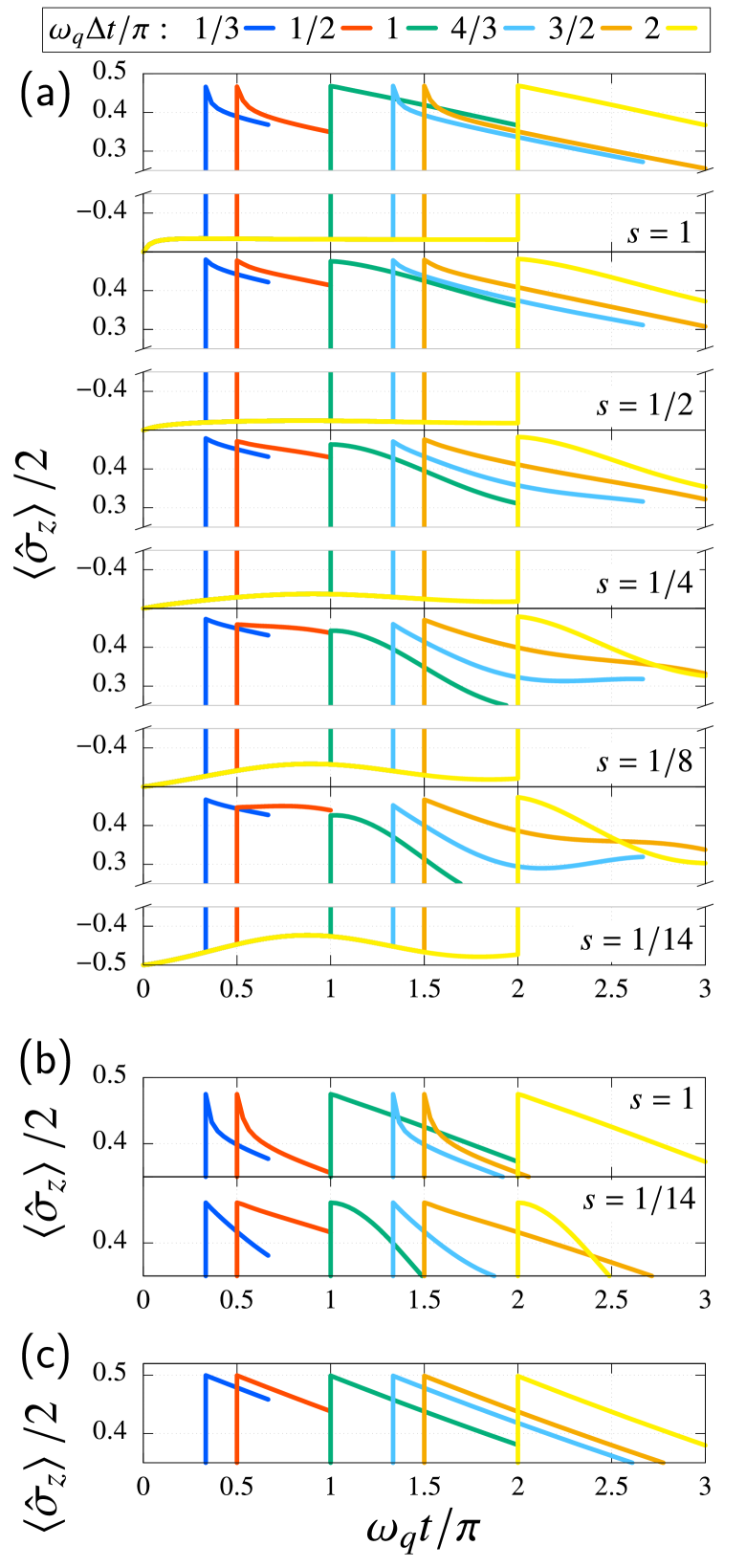
Figure 9: (a) Dynamics of the expectation value $\expectationvalue*{\hat{\sigma}_{z}(t)}/2$ during the sequence of three $R_{x}(\pi)$ gates, with various $\Delta t$ and a fixed $\Omega$ ($\Omega/\omega_{q}=\infty$). The vertical lines at the beginning and end of the sequence, which corresponds to the first and third pulse, are omitted. The initial states are the excited state, $\hat{\rho}_{0}=\hat{\rho}_{e}$. (b) Dynamics of $\expectationvalue*{\hat{\sigma}_{z}(t)}/2$ with the two idle phases interleaved with one impulsive pulse [Eq. (28)]. The initial states are the equilibrium state, $\hat{\rho}_{S}(0)=\hat{\rho}_{eq}$. As representatives, the dynamics with $s=1$ and $1/14$ are displayed. The dynamics of the first idle phase are not depicted, because the expectation value $\expectationvalue*{\hat{\sigma}_{z}(t)}$ takes a same value during this phase, as inferred by the equilibrium initial states. (c) Same dynamics as the case (a), but the dynamics are calculated with the Lindblad equation [Eq. (LABEL:eq:Lindblad)]. The dynamics during the first idle phase are not depicted. The results are independent of the spectral exponent $s$.

What happens when one simulates this situation within a Born–Markov treatment? This is seen in Fig. 9(c): For the application of the impulsive pulse, the unitary transformation, Eq. (15), is applied to the RDO, so that during the idle phases the dynamics follow from the Lindblad equation

$$\frac{\partial}{\partial t}\hat{\rho}_{S}(t)$$ (29)

$$= -\frac{i}{\hbar}\hat{H}^{\times}_{S}(\Omega=0,\phi;t)\hat{\rho}_{S}(t)$$ (30)

$$+2\pi S_{\beta}(\omega_{q})\left\{\hat{\sigma}_{-}\hat{\rho}_{S}(t)\hat{\sigma}_{+}-\frac{1}{2}\left(\hat{\sigma}_{+}\hat{\sigma}_{-}\right)^{\circ}\hat{\rho}_{S}(t)\right\}$$ (31)

$$+2\pi S_{\beta}(-\omega_{q})\left\{\hat{\sigma}_{+}\hat{\rho}_{S}(t)\hat{\sigma}_{-}-\frac{1}{2}\left(\hat{\sigma}_{-}\hat{\sigma}_{+}\right)^{\circ}\hat{\rho}_{S}(t)\right\}\,.$$ (32)

The parameter values for $S_{\beta}(\omega_{q})$ are identical to those of the HEOM calculations. Note that we have ignored the Lamb shift here because it does not contribute to the dynamics of the diagonal elements. We do not depict the dynamics during the first idle phase in Fig. 9(c) because the expectation value $\expectationvalue*{\hat{\sigma}_{z}(t)}/2$ in the equilibrium state of the bare system $\hat{\rho}_{S,eq}$ is very close to $-0.5$ and significant changes are not observed during this phase. In terms of the numerical calculation, the ADOs are always zero within the framework of the Lindblad equation, and therefore the time-dependent properties of the pulse application cannot be described. For this reason, the dynamics of the RDO during the second idle phase exhibits almost the same linear relaxation behavior irrespective of $\Delta t$.

We further mention that in the exact treatment with the HEOM, the total equilibrium state is sensitive to the direction of the rotation axis of the qubit due to the system–reservoir coupling. Namely, contributions of the terms $\hat{R}_{z}(\pm\omega_{q}t)$ in Eq. (15) can be expressed through the initial phase of the external field $\phi$, and the change of the time duration $\Delta t$ corresponds to the change of the direction of the rotation axis. This sensitivity is absent in the framework of the Born–Markov approximation approach and can thus not been predicted by this treatment. It is a clear signature of qubit–reservoir correlations.

We note in passing that in a previous study different dynamics of the RDO caused by different rotation axes were numerically predicted [24]. The cause of these differences is the same as the one for the $\pi$-periodicity in this study. For the dependence of the dynamics on $\Delta t$ with a finite amplitude $\Omega$, see Appendix E.3.

VI Fighting against decoherence

In this section, we present results of the Hahn-echo (HE) and dynamical-decoupling (DD) simulations as means to mitigate decoherence caused by phase errors due to sub-Ohmic reservoirs. Accordingly, in the sequel, we chose $\hat{V}=\hbar\hat{\sigma}_{z}$ as the system–reservoir interaction. The parameter values for the reservoir are the same as in the previous sections.

VI.1 Modeling

With respect to the modelling of the pulse sequence, we follow previous studies [51, 52, 53] and consider impulsive pulses so that the sequence of the HE is given by

$$\mathcal{U}_{\mathrm{i}}(\Delta t^{\prime})\mathcal{U}_{\mathrm{imp}}(\pi,0)\mathcal{U}_{\mathrm{i}}(\Delta t)\,,$$ (34)

while for the DD, a symmetric version of the Carr–Purcell–Meiboom–Gill (CPMG) sequence [54, 55] is applied, i.e.,

$$\Bigl{\{}\mathcal{U}_{\mathrm{i}}(\Delta t/2)\mathcal{U}_{\mathrm{imp}}(\pi,0)\mathcal{U}_{\mathrm{i}}(\Delta t)\mathcal{U}_{\mathrm{imp}}(\pi,0)\mathcal{U}_{\mathrm{i}}(\Delta t/2)\Bigr{\}}^{n}\quad$$ (35)

with integer $n>1$. The schematics of these sequences are displayed in Figs. 10(a) and 11(a), respectively. Note that we ignore the phase shift caused by the rotation $\hat{R}_{z}(\pm\omega_{\mathrm{ex}}t)$ in Eq. (15) in line with definitions in previous studies [32, 51, 52, 53]. Further, during the evolution in the idle phases, indicated by $\mathcal{U}_{\mathrm{i}}(\Delta t)$, the system Hamiltonian and the system part of the interaction Hamiltonian commute. Therefore, we can evaluate $\mathcal{U}_{\mathrm{i}}(\Delta t)\hat{\rho}_{\mathrm{tot}}(t)$ in a rigorous manner without introducing the ADOs, as discussed in Sec. II (see Appendix B.2 for more details).

As initial states we consider a factorized and a correlated state, respectively. The factorized one is defined as

$$\hat{\rho}^{\mathrm{f}}_{\mathrm{tot}}(0)= \hat{R}_{y}\left(-\frac{\pi}{2}\right)\outerproduct{0}{0}\hat{R}_{y}\left(\frac{\pi}{2}\right)\otimes\hat{\rho}_{R,eq}$$ (36)

$$= \frac{\left(\ket{0}+\ket{1}\right)\left(\bra{0}+\bra{1}\right)}{2}\otimes\hat{\rho}_{R,eq}\,,$$ (37)

and the correlated one as

$$\hat{\rho}^{\mathrm{c}}_{\mathrm{tot}}(0)=\hat{R}_{y}\left(-\frac{\pi}{2}\right)\frac{e^{-\beta\hat{H}_{\mathrm{tot}}}}{{\mathrm{tr}\{e^{-\beta\hat{H}_{\mathrm{tot}}}\}}}\hat{R}_{y}\left(\frac{\pi}{2}\right)\,.$$ (38)

In the latter preparation, all correlations due to the total equilibrium state $e^{-\beta\hat{H}_{\mathrm{tot}}}$ are taken into account.

In order to explore the impact of decoherence (dephasing), we evaluate the absolute value of the off-diagonal element of the reduced density operator $|\rho_{eg}(t)|=|\matrixelement{1}{\hat{\rho}_{S}(t)}{0}|$. Since it turns out that for the given set of parameters differences in the normalized dynamics $|\rho_{eg}(t)|/|\rho_{eg}(0)|$ between the factorized and correlated initial states are negligibly small, we only discuss the former case in detail. Note though that the effective Larmor frequency is renormalized, for details see Appendix D.2.

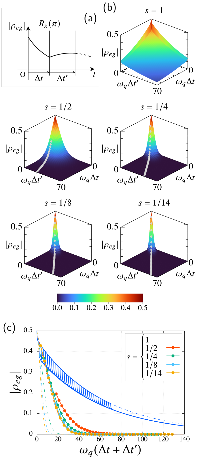
Figure 10: (a) Schematic of the Echo experiment. (b) Dynamics of the off-diagonal element $|\rho_{eg}(t)|$ during the echo experiments. The gray diamonds indicate a local maximum of $|\rho_{eg}(t)|$ with respect to $\Delta t^{\prime}$ with a fixed $\Delta t$. (c) Dynamics of the peak position and the whole dynamics of $|\rho_{eg}(t)|$ during the echo experiments. The filled circles correspond to the gray diamonds in (b). In the case for $s=1$, the whole dynamics of $|\rho_{eg}(t)|$ are depicted instead of the peak position. The dashed curves are the dynamics without the pulse (Ramsey experiments).

VI.2 Hahn echo (HE)

Figure 10(b) displays the dynamics of the off-diagonal element of the RDO, $|\rho_{eg}(t_{\mathrm{e}})|$ starting at $|\rho_{eg}(t_{\mathrm{e}}=0)|=1/2$. The time argument $t_{\mathrm{e}}$ is given by $t_{\mathrm{e}}=\Delta t+\Delta t^{\prime}$ [end of a single HE sequence, cf. Fig. 10(a)] with $\Delta t$ and $\Delta t^{\prime}$ being varied independently. Note that the curve along the line $\Delta t^{\prime}=0$ corresponds to the Ramsey experiments without the $R_{x}(\pi)$ pulse.

A general result of our simulations is that a recovery of $|\rho_{eg}(t)|$ is observed for sub-Ohmic reservoirs only, while the application of a pulse is always detrimental for Ohmic ones. In order to understand this, one has to recall that the echo technique was originally developed to reduce the effects of the “inhomogeneous broadening” in NMR experiments. This broadening results from the inhomogeneity of static magnetic fields which, within the framework of the system–reservoir model, corresponds to a time-independent two-time correlation function of the reservoir in the classical limit [56]. Now, for sub-Ohmic spectral densities the two-time correlator decays slower for smaller spectral exponents $s$ which is to say that the reservoir tends to become gradually more sluggish, as also depicted in Appendix C. Accordingly, in the Ohmic case ($s=1$), the relatively fast decay of the two-time correlation function is dominated by the large portion of higher frequency modes in the region $\omega_{q}\ll\omega\lesssim\omega_{c}$, leading to the fast decay of $|\rho_{eg}(t)|$ in the HE experiments. With the growing portion of low frequency modes in the spectral noise power, the strongly suppressed dynamics of the reservoir make it possible to mitigate the impact of decoherence by echo sequences. In order for this to be effective, the spectral exponent has to be lower than $s\approx 1/2$ since for this value the recovery is not yet observed in the short-time region $\omega_{q}\Delta t<14$ [cf. Fig. 11(c) with $s=1/2$ in which a fast decay right after the pulse application is found, which corresponds to the dynamics of the echo experiment around the time $\Delta t\simeq\Delta t^{\prime}$].

Table 1: Time constants of the decay of the off-diagonal element $|\rho_{eg}(t)|$ obtained from the Ramsey and echo experiments. The quantity $T_{\mathrm{R}}$ is the time constant of the Ramsey experiments, and $T_{\mathrm{E}}$ is the time constant of the echo experiments.

$s$	$1$	$1/2$	$1/4$	$1/8$	$1/14$
$\omega_{q}T_{\mathrm{R}}$	$62.5$	$16.9$	$7.82$	$5.39$	$4.46$
$\omega_{q}T_{\mathrm{E}}$	$62.5$	$27.7$	$19.6$	$17.2$	$16.5$

To investigate to which extent the echo sequence improves the qubit’s coherence time, we depict in Fig. 10(c) the maximum recovered value of $|\rho_{eg}(t)|$: For a fixed $\Delta t$, we detect local maxima with respect to $\Delta t^{\prime}$, and monitor the value of each local maximum as a function of the total time $\Delta t+\Delta t^{\prime}$. These results are then compared with those of Ramsey experiments ($\Delta t^{\prime}=0$). By way of example, in the Ohmic case ($s=1$), the whole dynamics of $|\rho_{eg}(t)|$ are instead displayed for various values of $\Delta t$ with the step-like decay corresponding to the pulse application. The time constants extracted from this analysis are listed in Table 1, see also Appendix F. As already mentioned above, in the Ohmic case, the intensity significantly decreases right after the pulse application, where the overall decay time remains almost the same. In contrast, in the sub-Ohmic cases, the improvement of the time constant is more significant with an increasing ratio $T_{\mathrm{E}}/T_{\mathrm{R}}$ for smaller spectral exponents. This implies that since the time-independent properties of the two-time correlation function are enhanced in the deep sub-Ohmic domain, the echo sequence works in a more efficient way. When the correlation function tends to be almost time-independent, the peak positions align along the diagonal in Fig. 10(b), again verifying that a deep sub-Ohmic reservoir behaves almost as a static reservoir on relevant timescales. Conversely, if we measure the signal with the condition $\Delta t=\Delta t^{\prime}$, the time constants decrease compared to what is depicted in Fig. 10(c).

Note that while the improvement of the time constant from the Ramsey to the HE experiments is the most significant in the case $s=1/14$, the absolute value of the time constant for the Ramsey experiment in this case is the smallest. Within the Born–Markov approximation, in the Ohmic and super-Ohmic cases, the decay rate due to decoherence, $1/T_{\mathrm{R}}$, is proportional to $S_{\beta}(0)$. In the sub-Ohmic case, however, the spectral noise power diverges at $\omega=0$, and this simple argument stemming from a perturbative treatment cannot be applied. In fact, the stronger divergence of $S_{\beta}(\omega)$ around $\omega\to 0$ for smaller exponents directly correlates with the tendency of $T_{\mathrm{R}}$.

VI.3 Dynamical decoupling (DD)

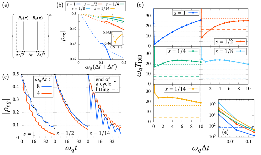
Figure 11: (a) Schematic of the CPMG sequence. (b) Dynamics of $|\rho_{eg}(t)|$ during the Hahn-echo experiments in the short-time region. The duration is given by $\omega_{q}\Delta t=0.1$. The dashed curve indicates the dynamics of the Ramsey experiments. In the inset, the same dynamics but with $\omega_{q}\Delta t=1$ and $s=1/14$ are plotted. (c) Dynamics of the off-diagonal element $|\rho_{eg}(t)|$ during the dynamical-decoupling experiments. As representatives, the cases $\omega_{q}\Delta t=4$ and $8$ for the spectral exponent $s=1$, $1/2$ and $1/14$ are depicted. The filled circles indicate the end of each cycle in the case $\omega_{q}\Delta t=8$, and the dashed curves are fitted exponential functions obtained from the values of the filled circles. (d) Time constant of the decay $T_{\mathrm{DD}}$ with respect to the duration of the idle phase $\Delta t$. In the sub-Ohmic case, the time constants for the Ramsey and echo experiments, $T_{\mathrm{R}}$ and $T_{\mathrm{E}}$, which are listed in Table 1, are also depicted as the dashed and dotted line, respectively. (e) Log–log plot of $T_{\mathrm{DD}}$ in the small-$\Delta t$ region. The time constants, $T_{\mathrm{R}}$ and $T_{\mathrm{E}}$, in the Ohmic case are depicted here as the dashed and dotted blue line, respectively.

Next, we study the dynamics during DD experiments with the pulse sequence shown in Fig. 11(a). Notably, while in previous studies [51, 52, 53, 26] only small to moderate durations $\Delta t$ have been considered, here, we explore a wide range of idle durations from small values much below the qubit frequency to relatively large values beyond, i.e., $0.002\leq\omega_{q}\Delta t\leq 10$.

By way of example, the dynamics with $\omega_{q}\Delta t=4$ and $\omega_{q}\Delta t=8$ for spectral exponents $s=1$, $1/2$, and $1/14$ are depicted in Fig. 11(c). Strikingly, one observes a different behavior for decreasing $s$ when $\Delta t$ grows: In the Ohmic regime a larger $\Delta t$ implies improved coherences while the opposite is true in the deep sub-Ohmic regime. In order to explore this quantitatively, we extract from these time traces time constants $T_{\mathrm{DD}}$ for the decay of coherences in the presence of DD with varying $\Delta t$ (for details see Appendix F) and depict them in Fig. 11(d).

In all cases, irrespective of the spectral exponent $s$, we can distinguish a domain for very short times $\omega_{q}\Delta t\ll 1$ with a steep drop of $T_{\mathrm{DD}}$ and a domain beyond with a much smoother behavior. In the latter domain the time constant $T_{\mathrm{DD}}$ increases and, deeper in the sub-Ohmic regime, approaches a local maximum before it tends to decrease again. The transition between these two time domains appears as a local minimum, the position of which shifts towards $\omega_{q}\Delta t\approx 1$ for decreasing spectral exponents.

In order to understand this behavior we first turn to the very-small-$\Delta t$ region. There, one can consider the simplified pulse sequence of the HE, as discussed above, since the HE sequence also appears in the fundamental pulse sequence for the DD, cf. Eqs. (34) and (35). Results are shown in Fig. 11(b) for $\omega_{q}\Delta t=0.1$. Apparently, in the very-short-time region after the application of a single Hahn-pulse a characteristic growth of coherences can be seen. In the short time regime $\omega_{c}\Delta t^{\prime}\ll 1$, the fluctuation of $\hat{V}$ caused by the reservoir can be seen as static, and thus the recovery of coherences is observed irrespective of the spectral exponent $s$. Right after this universal recovery of coherences, the system experiences decoherence when the duration of the first idle phase $\Delta t$ is small. This decoherence is similar to the universal decoherence[22, 57]: Due to the relation $[\hat{H}_{S},\hat{V}]=0$, the decay of the coherence is determined only by the properties of the reservoir, whose representation is the same as the one for the universal decoherence (see Appendix D.1.1). The universal decoherence is slower for deeper sub-Ohmic reservoirs which in turn leads to larger timescales for the universal recovery. By contrast, when $\Delta t$ increases, further recovery of coherence is observed for deep sub-Ohmic reservoirs, cf. inset of Fig. 11(b) for $\omega_{q}\Delta t=1$ with $s=1/14$: A fast increase of coherence in the region $1\leq\omega_{q}(\Delta t+\Delta t^{\prime})\leq 1.05$ is found and a subsequent slower increase, rather than universal decoherence, in the region $1.05\leq\omega_{q}(\Delta t+\Delta t^{\prime})$. We attribute the former steep increase to the universal behavior and the bending towards a slower increase to the recovery which is found in HE as well (we refer to this recovery as an HE-like recovery hereafter).

We conclude from this analysis that, if for a DD sequence, the next pulse is applied within this short time range, decoherence is indeed suppressed very efficiently. If the time between the first and the second pulse exceeds this time range, decoherence becomes substantial, very similar to what happens after application of a single HE.

Now, we turn to the analysis of the large-$\Delta t$ region, $\omega_{q}\Delta t\geq 0.2$. In the Ohmic case, steep drops in $|\rho_{eg}(t)|$ are observed in Fig. 11(c). This is due to the relatively large portion of high frequency modes in $S_{\beta}(\omega)$ as discussed above for the HE experiments. Larger values of $\Delta t$ lead to decreasing relevance of these modes and, consequently, the decay of coherence slows down as $\Delta t$ increases [left panel of Fig. 11(c), $s=1$]; it even reverts to an increasing time constant $T_{\mathrm{DD}}$ in the region $\omega_{q}\Delta t\geq 0.2$.

In the deep sub-Ohmic domain, the steep drops discussed above are no longer observed. Instead, the HE-like recovery of the intensity is observed in Fig. 11(c) leading to an improved coherence time even beyond what can be achieved with HE and what is observed in a Ramsey experiment (no pulses). Here, the strong presence of low frequency modes induces a smoother transition from the short to the moderate and the long time range. At $\omega_{q}\Delta t\approx 1$, the transition from the universal suppression of decoherence to the HE-like recovery appears. With increasing duration $\Delta t$ beyond the local minimum in $T_{\mathrm{DD}}$, decoherence between two successive pulses plays a significant role [right panel of Fig. 11(c)], and the time constant decreases. For example, in the case $s=1/14$, this results even in a local maximum at $\omega_{q}\Delta t=3$. The same discussion holds for the case $s=1/8$.

The cases with $s=1/2$ and $1/4$ are intermediate between those with $s=1$ and $1/14$: In Fig. 11(c) with $s=1/2$, the red curve displays the steep drop, although the magnitude of this decay is smaller in comparison to the case $s=1$. By contrast, the blue curve exhibits slight recoveries of the intensity in the middle and at the end of each cycle. This indicates that in the small-$\Delta t$ region, $0.2\leq\omega_{q}\Delta t\lesssim 4$, an improvement related to the fast decay is observed while in the longer $\Delta t$ region, $\omega_{q}\Delta t\gtrsim 5$, the HE-like recovery appears.

We thus draw the following conclusions: (i) The time constant $T_{\mathrm{DD}}$ strongly depends on the duration $\Delta t$ and the spectral exponent $s$. (ii) For Ohmic reservoirs, the DD-approach never improves the time constant compared to HE and Ramsey experiments, unless for extremely short times $\omega_{c}\Delta t<1$ with $\omega_{q}\ll\omega_{c}$. This corresponds to the “decoherence acceleration” found also in a previous study [53]. (iii) For sub-Ohmic spectral densities with $1/4<s\leq 1$ the application of DD is beneficial compared to Ramsey experiments but the time constant still remains below the one seen in HE except for very short times. (iv) In the relatively deep sub-Ohmic range $s\leq 1/4$, the DD provides an improvement of the stability of coherence beyond both the HE and Ramsey findings for almost all parameter values; a few exceptions are found in our results for $\omega_{q}\Delta t=0.2$ and $1$ with $s=1/4$.

As a final technical remark we mention that our simulations provide somewhat less accurate results in the very short time region $\omega_{q}\Delta t\leq 0.02$. As illustrated in Fig. 11(e), the decay is very slow in the region $\omega_{q}\Delta t\leq 0.02$ (orders of magnitudes larger $T_{\mathrm{DD}}$ than for longer time regions) so that numerical calculations are extremely susceptible to even tiny numerical errors. We observed, however, that the degrading accuracy of the results does not change the qualitative profile in Fig. 11(e), that is, the decrease of $T_{\mathrm{DD}}$ up to the duration $\omega_{q}\Delta t=0.2$ as well as the acceleration of decoherence for $\omega_{q}\Delta t\geq 0.02$ in the Ohmic case.

VII Summary and Conclusions

In this work, high-precision quantitative predictions are provided for various sequences of single-qubit gate operations for a broad class of thermal environments. Reservoirs with spectral densities of the form $J_{s}(\omega)\propto\omega^{s}$ are considered, i.e., from the Ohmic ($s=1$) to the deep sub-Ohmic ($s\ll 1$) domain, thus covering prominent noise sources for superconducting qubits such as electromagnetic fluctuations, two level fluctuators, and quasiparticle noise. As representative applications, gate sequences are chosen to consist of three pulses ($\pi$, $\pi/2$, and $H$ gate) of varying amplitudes separated by two idle phases of varying lengths. In this way, we are able to unfold a detailed and comprehensive picture of the dynamics and performance of major gate sequences for realistic superconducting circuit implementations in domains, where perturbative treatments (Lindblad, Redfield) fail. For this broad class of noisy environments we then analyze in detail the performance of quantum control techniques (Hahn echo, dynamical decoupling) to mitigate decoherence. Our work clearly demonstrates the necessity to invoke highly advanced simulations techniques such as the HEOM to provide a detailed understanding of the intricate qubit–reservoir dynamics and to deliver quantitative predictions for complex gate operations matching the growing accuracy achieved experimentally.

The main results can be summarized as follows:

1. In the temperature domain, where superconducting qubits are operated, retardation effects of the reservoir induce long-range correlations during gate sequences, particularly between subsequent idle phases. This impact grows for reservoirs with more prominent sub-Ohmic characteristics (low to moderate frequency noise compared to qubit transition frequencies).

2. By varying parameters of gate sequences (amplitude/pulse duration, duration of idle phase) and depending on spectral exponents of reservoirs, we found a non-monotonous pattern for gate fidelities for all three initial preparations (ground, excited, and thermal state). In contrast to simple expectations, the recovery of fidelities in subsequent idle phases originates from non-Markovian dynamics of $\hat{\rho}_{S}(t)$. By choosing proper parameters in each of these cases, our simulations lay the foundation for optimizing gate performances.

3. In most cases, we observed that fidelities for gate sequences starting from the qubit’s ground state or thermal state exceed those starting from the excited state.

4. Fidelities after the final pulse, decisive for the overall gate performance, strongly depend on the loss or recovery of fidelities during all preceding idle phases.

5. The rotation axis of qubit gate operations on the Bloch sphere relative to the qubit–reservoir coupling has substantial influence on gate performances, as explicitly demonstrated for $R_{x}(\pi/2)$ and $H$ gates.

6. Long-range qubit–reservoir correlations were shown to induce inter-phase correlations during gate sequences depending on the relative portion of low frequency modes in the reservoirs. Monitoring the qubit’s population dynamics upon application of impulse $R_{x}(\pi)$ gates interleaved by idle phases of varying lengths allows us to reveal directly the significance of non-Markovian feedback in actual circuits. The latter appears to be imprinted in periodicities that are predicted to occur when comparing the qubit dynamics for idle phases $\omega_{q}\Delta t$ that differ by multiples of $\pi$.

7. Two established schemes to reduce the impact of decoherence due to dephasing [Hahn echo (HE) and dynamical decoupling (DD)] turned out to be beneficial in certain ranges of parameter space only. For the HE as well as DD, coherences are stabilized dominantly for sub-Ohmic reservoirs, roughly for those with spectral exponents $s<1/2$. There, the HE leads to gradually increasing improvements when moving towards the deep sub-Ohmic domain, where decoherence most drastically reduces coherence times. For the DD, in this domain and for pulse lengths on the order of the qubit transition frequency, local maxima appear around which coherence times are substantially enhanced compared to simple Ramsey results. For short DD pulse lengths (sufficiently shorter than the timescales for qubit transition frequencies and on the order or below the scale for reservoir cut-off frequencies), a regime of universal recovery of coherences can be seen.

8. The developed and applied rigorous numerical simulation technique is highly efficient and very versatile so that it can be used in the lab to directly guide optimized designs of circuitries and gate pulse shapes. For example, the results reported here for a single run (a single cell in Fig. 4) were obtained on a personal computer (Intel Core i9 CPU with $10$ cores) within a few seconds (Ohmic case) up to a few hours (very deep sub-Ohmic case). This can be further improved by implementing Matrix Product State (MPS) techniques within the FP-HEOM [28].

In this paper, we restricted ourselves to the simulations of single qubit gates. The pulse shape was also restricted to a rotating external field, with the ideal switching given by a step function. This can easily be extended by taking into account derivative removal adiabatic gates (DRAG) [58] with a finite rise time. Leakage effects of pulses to the second and higher qubit excited states have also not been considered. However, due to its unique efficiency combined with its versatile applicability the presented numerical approach allows us to investigate these topics as well. Future extensions include two-qubit gate operations, circuitries with more complex impedances, and multi-qubit correlations.

Appendix A Rotation operators and time evolution

In this appendix, we discuss in detail the rotation operators and Hamiltonian. Following the main text, we move to the rotating frame with the rotation axis and angular frequency given by $z$ and $\omega_{\mathrm{ex}}$, respectively. The system Hamiltonian is transformed as

$$\tilde{H}_{S}(\Omega,\phi)$$ (39)

$$= \hat{R}_{z}(-\omega_{\mathrm{ex}}t)\hat{H}_{S}(\Omega,\phi;t)\hat{R}_{z}(\omega_{\mathrm{ex}}t)+i\hbar\dot{\hat{R}}_{z}(-\omega_{\mathrm{ex}}t)\hat{R}_{z}(\omega_{\mathrm{ex}}t)$$ (40)

$$= \frac{\hbar(\omega_{q}-\omega_{\mathrm{ex}})}{2}\hat{\sigma}_{z}+\frac{\hbar\Omega}{2}\left(\hat{\sigma}_{x}\cos\phi+\hat{\sigma}_{y}\sin\phi\right)\,.$$ (41)

Note that the system Hamiltonian in the rotating frame is time-independent, and we omit the argument $t$ for $\tilde{H}_{S}$. When we choose $\omega_{q}$ for the frequency $\omega_{\mathrm{ex}}$, as discussed in the main text, the first term of this equation vanishes. Under this condition, we can easily confirm the relations $\tilde{H}_{S}(\Omega,0)=\hbar\Omega\hat{\sigma}_{x}/2$ and $\tilde{H}_{S}(\Omega,\pi/2)=\hbar\Omega\hat{\sigma}_{y}/2$. This indicates that we can express the rotation operator with the time-evolution operator as

$$\hat{R}_{x}(\theta) =\exp\left[-\frac{i}{\hbar}\tilde{H}_{S}(\Omega,0)\tau\right]\,,$$ (42)

$$\hat{R}_{y}(\theta) =\exp\left[-\frac{i}{\hbar}\tilde{H}_{S}\left(\Omega,\frac{\pi}{2}\right)\tau\right]\,,$$ (43)

where the frequency of the external field $\omega_{\mathrm{ex}}$ is set to $\omega_{q}$. Note that the pulse duration $\tau$ is determined with the condition $\tau=\theta/\Omega$. Accordingly, we can obtain the rotation operators with the negative angle with $\phi=\pi$ for the $x$-axis rotation and $\phi=-\pi/2$ for the $y$-axis rotation. A rotation operator about an arbitrary axis in the $x$–$y$ plane is expressed as $\hat{R}_{\phi}(\theta)=\exp[-i\theta(\hat{\sigma}_{x}\cos\phi+\hat{\sigma}_{y}\sin\phi)/2]$ and corresponds to the time-evolution operator $\exp[-i\tilde{H}_{S}(\Omega,\phi)\tau/\hbar]$.

By using the relation

$$\exp\left[-\frac{i}{\hbar}\tilde{H}_{S}(\Omega,\phi)\tau\right]$$ (44)

$$= \hat{R}_{z}(-\omega_{q}[t+\tau])\exp\left[-\frac{i}{\hbar}\int_{t}^{t+\tau}dt^{\prime}\hat{H}_{S}(\Omega,\phi;t^{\prime})\right]$$ (45)

$$\times\hat{R}_{z}(\omega_{q}t)\,,$$ (46)

which transforms the time-evolution operator in the rotating frame to that in the laboratory frame, the rotation operator in the rotating frame is expressed as

$$\tilde{\rho}_{S}(t+\tau)= \hat{R}_{\phi}(\theta)\tilde{\rho}_{S}(t)\hat{R}_{\phi}(-\theta)$$ (47)

$$= \exp\left[-\frac{i}{\hbar}\tilde{H}_{S}(\Omega,\phi)\tau\right]\tilde{\rho}_{S}(t)\exp\left[\frac{i}{\hbar}\tilde{H}_{S}(\Omega,\phi)\tau\right]$$ (48)

$$= \hat{R}_{z}(-\omega_{q}[t+\tau])\exp[-\frac{i}{\hbar}\int_{t}^{t+\tau}dt^{\prime}\hat{H}_{S}(\Omega,\phi;t^{\prime})]$$ (49)

$$\times\hat{R}_{z}(\omega_{q}t)\tilde{\rho}_{S}(t)\hat{R}_{z}(-\omega_{q}t)$$ (50)

$$\times\exp\left[\frac{i}{\hbar}\int_{t}^{t+\tau}dt^{\prime}\hat{H}_{S}(\Omega,\phi;t^{\prime})\right]\hat{R}_{z}(\omega_{q}[t+\tau])\,.$$ (51)

Using the relation $\hat{\rho}_{S}(t)=\hat{R}_{z}(\omega_{q}t)\tilde{\rho}_{S}(t)\hat{R}_{z}(-\omega_{q}t)$, we obtain the rotation operator corresponding to the time evolution with the Hamiltonian in Eq. (LABEL:eq:H_S) in the laboratory frame. We utilize the laboratory frame to introduce the reservoir operators. Accordingly, the system Hamiltonian in Eq. (51) is replaced with $\hat{H}_{\mathrm{tot}}(\Omega,\phi;t)=\hat{H}_{S}(\Omega,\phi;t)-\hat{V}\hat{X}+\hat{H}_{R}$, and the time-evolution operator is expressed by Eq. (7). The density operator is also replaced with $\hat{\rho}_{\mathrm{tot}}(t)$. There is no reason to assume that the reservoir rotates about the $z$ axis at the angular frequency $\omega_{q}$, and it is plausible that the qubit system couples with the reservoir in this form.

Next, we consider the application of impulsive pulses. As mentioned in the main text, we can ignore the system–reservoir coupling term when we consider the impulsive pulses. Equation (51) is then rewritten as

$$\tilde{\rho}_{\mathrm{tot}}(t+\tau)= \exp\left[-\frac{i}{\hbar}\left(\tilde{H}_{S}(\Omega,\phi)+\hat{H}_{R}\right)\tau\right]\tilde{\rho}_{\mathrm{tot}}(t)$$ (52)

$$\times\exp\left[\frac{i}{\hbar}\left(\tilde{H}_{S}(\Omega,\phi)+\hat{H}_{R}\right)\tau\right]$$ (53)

$$= e^{-i\hat{H}_{R}\tau/\hbar}\hat{R}_{\phi}(\theta)\tilde{\rho}_{\mathrm{tot}}(t)\hat{R}_{\phi}(-\theta)e^{i\hat{H}_{R}\tau/\hbar}\,.$$ (54)

Note that the transformation with $\hat{R}_{z}(-\omega_{q}t)$ does not change the reservoir Hamiltonian. For the impulsive pulse, we take the limits $\Omega\to\infty$ and $\tau\to 0$, keeping $\theta$ a finite fixed value. With this operation, we obtain the equation for the application of the impulsive pulse in the rotating frame as follows:

$$\tilde{\rho}_{\mathrm{tot}}(t)\leftarrow \hat{R}_{\phi}(\theta)\tilde{\rho}_{\mathrm{tot}}(t)\hat{R}_{\phi}(-\theta)\,.$$ (55)

When we go back to the laboratory frame from the rotating frame, we obtain Eq. (15).

Appendix B Details of the HEOM

B.1 Derivation of the HEOM

In this appendix, we illustrate the detailed derivation of the HEOM. The total Hamiltonian consisting of the system and reservoir is described with

$$\hat{H}_{\mathrm{tot}}(\Omega,\phi;t)$$ (56)

$$= \hat{H}_{S}(\Omega,\phi;t)-\hat{V}\hat{X}+\hat{H}_{R}$$ (57)

$$= \hat{H}_{S}(\Omega,\phi;t)-\hat{V}\sum_{j}c_{j}\hat{x}_{j}+\sum_{j}\left(\frac{\hat{p}_{j}^{2}}{2m_{j}}+\frac{1}{2}m_{j}\omega_{j}^{2}\hat{x}_{j}^{2}\right)\,.$$ (58)

The reservoir is represented by an infinite number of harmonic oscillators, and $\hat{p}_{j},\hat{x}_{j},m_{j}$ and $\omega_{j}$ are the momentum, position, mass and angular frequency of the $j$th bath, respectively. The coupling strength between the system and $j$th bath is given by $c_{j}$, which defines the spectral density as

$$J(\omega)=\sum_{j}\frac{c^{2}_{j}}{2m_{j}\omega_{j}}\delta(\omega-\omega_{j})\,.$$ (59)

The system part of the coupling $\hat{V}$ is set to $\hbar\hat{\sigma}_{x}$ and $\hbar\hat{\sigma}_{z}$, as discussed in the main text.

To obtain the equation for the open quantum dynamics without any approximations, we exploit the Feynman–Vernon path integral representation. The reduced density operator (RDO) of the system, $\hat{\rho}_{S}(t)=\mathrm{tr}_{R}\{e^{-i\hat{H}_{\mathrm{tot}}t/\hbar}\hat{\rho}_{\mathrm{tot}}(0)e^{i\hat{H}_{\mathrm{tot}}t/\hbar}\}$, is expressed as

$$\matrixelement{\mu}{\hat{\rho}_{S}(t)}{\mu^{\prime}}$$ (60)

$$= \int\frac{d^{2}\mu_{i}d^{2}\mu^{\prime}_{i}}{N(\mu_{i})N(\mu^{\prime}_{i})}\int_{\mu(0)=\mu_{i}}^{\mu(t)=\mu}\mathcal{D}[\mu(\cdot)]\int_{\mu^{\prime}(0)=\mu^{\prime}_{i}}^{\mu^{\prime}(t)=\mu^{\prime}}\mathcal{D}[\mu^{\prime}(\cdot)]$$ (61)

$$\times\exp\left[\frac{i}{\hbar}\int_{0}^{t}dt^{\prime}L_{S}(\mu;t^{\prime})-\frac{i}{\hbar}\int_{0}^{t}dt^{\prime}L_{S}(\mu^{\prime};t^{\prime})\right]$$ (62)

$$\times\matrixelement{\mu_{i}}{\hat{\rho}_{S}(0)}{\mu^{\prime}_{i}}\mathscr{F}[\mu,\mu^{\prime};t]\,.$$ (63)

Here, we consider the spin-coherent state $\ket{\mu}$ [59], and $L_{S}(\mu;t)$ is the Lagrangian of the system. The functional $\mathscr{F}[\mu,\mu^{\prime};t]$ is the influence functional, which is given by

$$\mathscr{F}[\mu,\mu^{\prime};t]$$ (64)

$$= \exp[-\frac{1}{\hbar^{2}}\int_{0}^{t}dt^{\prime}\int_{0}^{t^{\prime}}dt^{\prime\prime}V^{\times}(\mu,\mu^{\prime};t^{\prime})$$ (65)

$$\times\{C(t^{\prime}\!-\!t^{\prime\prime})V(\mu;t^{\prime\prime})-C^{*}(t^{\prime}\!-\!t^{\prime\prime})V(\mu^{\prime};t^{\prime\prime})\}\biggr{]}$$ (66)

$$= \exp[-\frac{1}{\hbar^{2}}\int_{0}^{t}dt^{\prime}\int_{0}^{t^{\prime}}dt^{\prime\prime}V^{\times}(\mu,\mu^{\prime};t^{\prime})$$ (67)

$$\times\{C^{\prime}(t^{\prime}\!-\!t^{\prime\prime})V^{\times}(\mu,\mu^{\prime};t^{\prime\prime})+iC^{\prime\prime}(t^{\prime}\!-\!t^{\prime\prime})V^{\circ}(\mu,\mu^{\prime};t^{\prime\prime})\biggr{]}\,.$$ (68)

The quantity $1/N(\mu)=2/\{\pi(1+|\mu|^{2})^{2}\}$ is the normalization factor for the spin-coherent states. The function $V(\mu;t)$ is the path-integral representation of the operator $\hat{V}$, and $V^{\times}(\mu,\mu^{\prime};t)=V(\mu;t)-V(\mu^{\prime};t)$ and $V^{\circ}(\mu,\mu^{\prime};t)=V(\mu;t)+V(\mu^{\prime};t)$ are the corresponding commutator and anticommutator, respectively. The Lagrangian of the system $L_{S}(\mu;t)$ is also defined in the path-integral representation. For more details of the path integral in the spin-coherent representation, we refer the readers to Ref. 60. The function $C^{*}(t)$ indicates the complex conjugate of $C(t)$, and we have utilized the relation $C^{*}(t)=C(-t)$ to obtain the expression of Eq. (68). The real and imaginary part of the two-time correlation function is defined as $C(t)=C^{\prime}(t)+iC^{\prime\prime}(t)$. Here, we assume the factorized initial state $\hat{\rho}_{\mathrm{tot}}(0)=\hat{\rho}_{S}(0)\otimes\hat{\rho}_{R,eq}$.

We express the two-time correlation function $C(t)$ with the complex-valued exponential functions [Eq. (18)]. The original Free-Pole HEOM (FP-HEOM) [28] is based on the representation of Eq. (66), and its form is expressed in Eq. (20), where the auxiliary density operators (ADOs) are not Hermitian operators. In this paper, we derive the HEOM with Hermitian ADOs to reduce the computational costs. To achieve this goal, we utilize the representation of Eq. (68) and the generalized form of the HEOM [61].

First, we expand Eq. (18) in the following form:

$$C(t)= \sum_{k=1}^{K}e^{-\gamma_{k}t}\{d^{\prime}_{k}\cos\omega_{k}t+d^{\prime\prime}_{k}\sin\omega_{k}t\}$$ (69)

$$+i\sum_{k=1}^{K}e^{-\gamma_{k}t}\{d^{\prime\prime}_{k}\cos\omega_{k}t-d^{\prime}_{k}\sin\omega_{k}t\}$$ (70)

$$= \sum_{k=1}^{K}\{\phi_{k}(t)+i\psi_{k}(t)\}\,.$$ (71)

Here, we have introduced the real and imaginary part of the coefficient $d_{k}$ as $d_{k}=d^{\prime}_{k}+id^{\prime\prime}_{k}$. Utilizing the super-operator

$$\Theta_{k}(\mu,\mu^{\prime};t,s)= \phi_{k}(t-s)\frac{-i}{\hbar}V^{\times}(\mu,\mu^{\prime};s)$$ (72)

$$+\psi_{k}(t-s)\frac{1}{\hbar}V^{\circ}(\mu,\mu^{\prime};s)$$ (73)

for $k=1,\ldots,K$, we can express the influence functional in Eq. (68) as

$$\mathscr{F}[\mu,\mu^{\prime};t]$$ (74)

$$= \exp\left[\int_{0}^{t}\!\!dt^{\prime}\int_{0}^{t^{\prime}}\!\!dt^{\prime\prime}\frac{-i}{\hbar}V^{\times}(\mu,\mu^{\prime};t^{\prime})\sum_{k=1}^{K}\Theta_{k}(\mu,\mu^{\prime};t^{\prime},t^{\prime\prime})\right]\,.$$ (75)

By introducing $\bar{\Theta}_{k}(\mu,\mu^{\prime};t,s)$ as

$$\bar{\Theta}_{k}(\mu,\mu^{\prime};t,s)= \bar{\phi}_{k}(t-s)\frac{-i}{\hbar}V^{\times}(\mu,\mu^{\prime};s)$$ (76)

$$+\bar{\psi}_{k}(t-s)\frac{1}{\hbar}V^{\circ}(\mu,\mu^{\prime};s)\,,$$ (77)

where $\bar{\phi}_{k}(t)$ and $\bar{\psi}_{k}(t)$ are given by

$$\bar{\phi}_{k}(t)= e^{-\gamma_{k}t}\{-d^{\prime}_{k}\sin\omega_{k}t+d^{\prime\prime}_{k}\cos\omega_{k}t\}\,,$$ (78)

$$\bar{\psi}_{k}(t)= -e^{-\gamma_{k}t}\{d^{\prime\prime}_{k}\sin\omega_{k}t+d^{\prime}_{k}\cos\omega_{k}t\}\,,$$ (79)

we obtain the following equation:

$$\begin{aligned} \frac{\partial}{\partial t}\Theta_{k}(\mu,\mu^{\prime};t,s)&\!=\!-\gamma_{k}\Theta_{k}(\mu,\mu^{\prime};t,s)\!+\!\omega_{k}\bar{\Theta}_{k}(\mu,\mu^{\prime};t,s)\,,\\ \frac{\partial}{\partial t}\bar{\Theta}_{k}(\mu,\mu^{\prime};t,s)&\!=\!-\gamma_{k}\bar{\Theta}_{k}(\mu,\mu^{\prime};t,s)\!-\!\omega_{k}\Theta_{k}(\mu,\mu^{\prime};t,s)\,.\end{aligned}\quad$$ (80)

Defining the ADO and its time derivative as

$$\matrixelement{\mu}{\hat{\rho}_{\vec{m},\vec{n}}(t)}{\mu^{\prime}}= \int\frac{d^{2}\mu_{i}d^{2}\mu^{\prime}_{i}}{N(\mu_{i})N(\mu^{\prime}_{i})}\int_{\mu(0)=\mu_{i}}^{\mu(t)=\mu}\mathcal{D}[\mu(\cdot)]\int_{\mu^{\prime}(0)=\mu^{\prime}_{i}}^{\mu^{\prime}(t)=\mu^{\prime}}\mathcal{D}[\mu^{\prime}(\cdot)]$$ (81)

$$\times\prod_{k=1}^{K}\frac{1}{\sqrt{m_{k}!n_{k}!}}\left(\int_{0}^{t}dt^{\prime\prime}\Theta_{k}(\mu,\mu^{\prime};t,t^{\prime\prime})\right)^{m_{k}}\left(\int_{0}^{t}dt^{\prime\prime}\bar{\Theta}_{k}(\mu,\mu^{\prime};t,t^{\prime\prime})\right)^{n_{k}}$$ (82)

$$\times\exp\left[\frac{i}{\hbar}\int_{0}^{t}dt^{\prime}L_{S}(\mu;t^{\prime})-\frac{i}{\hbar}\int_{0}^{t}dt^{\prime}L_{S}(\mu^{\prime};t^{\prime})\right]\matrixelement{\mu_{i}}{\hat{\rho}_{S}(0)}{\mu^{\prime}_{i}}\mathscr{F}[\mu,\mu^{\prime};t]$$ (83)

and

$$\frac{\partial\hat{\rho}_{\vec{m},\vec{n}}(t)}{\partial t}=\int\frac{d^{2}\mu d^{2}\mu^{\prime}}{N(\mu)N(\mu^{\prime})}\ket{\mu}\lim_{\Delta t\to 0}\frac{\matrixelement{\mu}{\hat{\rho}_{\vec{m},\vec{n}}(t+\Delta t)}{\mu^{\prime}}-\matrixelement{\mu}{\hat{\rho}_{\vec{m},\vec{n}}(t)}{\mu^{\prime}}}{\Delta t}\bra{\mu^{\prime}}\,,$$ (84)

respectively, we obtain the HEOM in the following form through the use of Eq. (80):

$$\frac{\partial}{\partial t}\hat{\rho}_{\vec{m},\vec{n}}(t)= -\frac{i}{\hbar}\hat{H}^{\times}_{S}(\Omega,\phi;t)\hat{\rho}_{\vec{m},\vec{n}}(t)-\sum_{k=1}^{K}(m_{k}+n_{k})\gamma_{k}\hat{\rho}_{\vec{m},\vec{n}}(t)$$ (85)

$$+\sum_{k=1}^{K}\omega_{k}\Bigl{\{}\sqrt{m_{k}(n_{k}+1)}\hat{\rho}_{\vec{m}-\vec{e}_{k},\vec{n}+\vec{e}_{k}}(t)-\sqrt{(m_{k}+1)n_{k}}\hat{\rho}_{\vec{m}+\vec{e}_{k},\vec{n}-\vec{e}_{k}}(t)\Bigr{\}}$$ (86)

$$-\frac{i}{\hbar}\hat{V}^{\times}\sum_{k=1}^{K}\sqrt{m_{k}+1}\hat{\rho}_{\vec{m}+\vec{e}_{k},\vec{n}}(t)$$ (87)

$$+\sum_{k=1}^{K}\left[\sqrt{m_{k}}\left\{-\frac{id^{\prime}_{k}}{\hbar}\hat{V}^{\times}+\frac{d^{\prime\prime}_{k}}{\hbar}\hat{V}^{\circ}\right\}\hat{\rho}_{\vec{m}-\vec{e}_{k},\vec{n}}(t)+\sqrt{n_{k}}\left\{-\frac{id^{\prime\prime}_{k}}{\hbar}\hat{V}^{\times}-\frac{d^{\prime}_{k}}{\hbar}\hat{V}^{\circ}\right\}\hat{\rho}_{\vec{m},\vec{n}-\vec{e}_{k}}(t)\right].$$ (88)

The vector $\vec{e}_{k}$ is the unit vector of the $k$th element, and $\hat{\rho}_{\vec{0},\vec{0}}(t)$ corresponds to the RDO $\hat{\rho}_{S}(t)$. The symbols $\times$ and $\circ$ denote the commutator and anticommutator respectively, as $\hat{O}_{1}^{\times}\hat{O}_{2}=\hat{O}_{1}\hat{O}_{2}-\hat{O}_{2}\hat{O}_{1}$ and $\hat{O}^{\circ}_{1}\hat{O}_{2}=\hat{O}_{1}\hat{O}_{2}+\hat{O}_{2}\hat{O}_{1}$. Note that the last line of Eq. (88) corresponds to $\Theta(\mu,\mu^{\prime};t,t)$ and $\bar{\Theta}(\mu,\mu^{\prime};t,t)$. Furthermore, the third and fourth line of Eq. (88) correspond to $\mathcal{L}_{k}^{+}$ and $\mathcal{L}_{k}^{-}$ in Eq. (20), respectively. The super-operator $\mathcal{L}_{S}$ in Eq. (20) is defined as $\mathcal{L}_{S}=\hat{H}_{S}^{\times}(\Omega,\phi;t)/\hbar$ in Eq. (88). The dynamics following from Eqs. (20) and (88) are same, but Eq. (88) is computationally more advantageous due to the Hermitian ADOs; we only need to treat upper (or lower) triangular elements of density matrices. Computationally, we can exploit this advantage through the use of (generalized) Bloch-vector representation [62].

B.2 The path-integral representation of the RDO for pure dephasing simulations

In this subsection, we derive an equation for the RDO controlled by the Hahn-echo and dynamical-decoupling schemes, which was discussed in Sec. VI. In those simulations, we only considered the impulsive pulses, and therefore we only need to consider the time evolution of the idle phases. For the phase error, the total Hamiltonian in Eq. (58) during the idle phase is given by $\hat{H}_{\mathrm{tot}}=\hbar\omega_{q}\hat{\sigma}_{z}/2-\hbar\hat{\sigma}_{z}\hat{X}+\hat{H}_{R}$. When we introduce the eigenvectors of the system Hamiltonian, $\hat{\sigma}_{z}\ket{a}=(-1)^{a+1}\ket{a}$ ($a=0,1$), and the eigenvectors of the position operator of the reservoir, $\ket{\bm{x}}=\ket{x_{1},\ldots,x_{j},\ldots}$, the time-evolution operator is evaluated as

$$\matrixelement{b,\bm{x}^{\prime}}{e^{-i\hat{H}_{\mathrm{tot}}t/\hbar}}{a,\bm{x}}$$ (89)

$$= \delta_{ab}e^{-i\omega_{a}t}\matrixelement{\bm{x}^{\prime}}{\exp\left[-\frac{i}{\hbar}\left(\hat{H}_{R}-(-1)^{a+1}\hbar\hat{X}\right)t\right]}{\bm{x}}\,,$$ (90)

where $\delta_{ab}$ is the Kronecker delta and $\omega_{a}=(-1)^{a+1}\omega_{q}/2$. The Boltzmann distribution $e^{-\beta\hat{H}_{\mathrm{tot}}}$ is also evaluated in the same way with the replacement of $it/\hbar$ with $\beta$. Note that the system part of the total Hamiltonian is replaced with $c$-numbers, and the bracket only includes the reservoir operators. Considering the time evolution, $e^{-i\hat{H}_{\mathrm{tot}}t/\hbar}\hat{\rho}^{\mathrm{c}}_{\mathrm{tot}}(0)e^{i\hat{H}_{\mathrm{tot}}t/\hbar}$, where $\hat{\rho}^{\mathrm{c}}_{\mathrm{tot}}(0)$ is given by Eq. (38), we obtain the matrix element of the RDO $\rho_{ab}(t)=\matrixelement{a}{\hat{\rho}_{S}(t)}{b}$ in the following form by tracing out the reservoir degrees of freedom:

$$\rho_{ab}(t)$$ (91)

$$= e^{-i\omega_{ab}t}\sum_{c}\matrixelement{a}{\hat{R}_{y}\left(-\frac{\pi}{2}\right)}{c}\frac{e^{-\beta\hbar\omega_{c}}}{Z}\matrixelement{c}{\hat{R}_{y}\left(\frac{\pi}{2}\right)}{b}$$ (92)

$$\times\exp[\begin{aligned} &-\int_{0}^{t}dt^{\prime}\int_{0}^{t^{\prime}}dt^{\prime\prime}v_{ab}^{2}C^{\prime}(t^{\prime}-t^{\prime\prime})\\ &+i\int_{0}^{t}dt^{\prime}\int_{0}^{\beta\hbar}d\tau^{\prime}v_{ab}\bar{C}(-t^{\prime}-i\tau^{\prime})(-1)^{c+1}\biggr{]}\,,\end{aligned}$$ (93)

where $\omega_{ab}=\omega_{a}-\omega_{b}$ is the difference of the frequency between the bra- and ket-vectors, and $Z=\mathrm{tr}\{e^{-\beta\hat{H}_{S}}\}=2\cosh(\beta\hbar\omega_{q}/2)$ is the partition function of the bare system.

The first term of the exponent corresponds to the influence functional in Eq. (68), and $v_{ab}=(-1)^{a+1}-(-1)^{b+1}$ corresponds to the commutator. Note that $V(\mu;t)$ and $V(\mu^{\prime};t)$ are replaced with $\hbar(-1)^{a+1}$ and $\hbar(-1)^{b+1}$, respectively. The term $V^{\times}(\mu,\mu^{\prime};t^{\prime})V^{\circ}(\mu,\mu^{\prime};t^{\prime\prime})$ in Eq. (68) vanishes here.

The second term of the exponent is originated from the correlated initial state and describes correlations between the Boltzmann distribution of the total Hamiltonian $e^{-\beta\hat{H}_{\mathrm{tot}}}$ and the time-evolution operator $e^{\pm i\hat{H}_{\mathrm{tot}}t/\hbar}$. The extended two-time correlation function is defined as

$$\bar{C}(z)=\hbar\int_{0}^{\infty}d\omega J(\omega)\frac{\cosh\left(\frac{\beta\hbar\omega}{2}-i\omega z\right)}{\sinh\left(\frac{\beta\hbar\omega}{2}\right)}\,.$$ (95)

If the variable $z$ is a real number, $z\in\mathbb{R}$, the function $\bar{C}(z)$ coincides with $C(t)$.

Note that the influence functional with the correlated initial state additionally includes the term

$$\exp\left[\frac{1}{\hbar^{2}}\int_{0}^{\beta\hbar}d\tau^{\prime}\int_{0}^{\tau^{\prime}}d\tau^{\prime\prime}V(\bar{\mu};\tau^{\prime})\bar{C}(-i\tau^{\prime}+i\tau^{\prime\prime})V(\bar{\mu};\tau^{\prime\prime})\right]\,.$$ (96)

In our case, the term $V(\bar{\mu};\tau^{\prime})V(\bar{\mu};\tau^{\prime\prime})$ is replaced with $\hbar^{2}(-1)^{2c+2}=\hbar^{2}$, and the above is expressed by $e^{-\beta\lambda}$, where $\lambda=\hbar^{2}\int_{0}^{\infty}d\omega J(\omega)/\omega$ is the reorganization energy. This term only shifts the origin of the energy and is omitted with the normalization condition at $t=0$.

For the Hahn-echo experiment, the pulse sequence in the super-operator representation is given by Eq. (34), and corresponding time evolution is evaluated as

$$\matrixelement{b,\bm{x}^{\prime}}{e^{-i\hat{H}_{\mathrm{tot}}\Delta t^{\prime}/\hbar}\hat{R}_{x}(\pi)e^{-i\hat{H}_{\mathrm{tot}}\Delta t/\hbar}}{a,\bm{x}}$$ (97)

$$= e^{-i(\omega_{b}\Delta t^{\prime}+\omega_{a}\Delta t)}\matrixelement{b}{\hat{R}_{x}(\pi)}{a}$$ (98)

$$\times\biggl{\langle}\bm{x}^{\prime}\biggr{|}\exp\left[-\frac{i}{\hbar}\left(\hat{H}_{R}-(-1)^{b+1}\hbar\hat{X}\right)\Delta t^{\prime}\right]$$ (99)

$$\times\exp\left[-\frac{i}{\hbar}\left(\hat{H}_{R}-(-1)^{a+1}\hbar\hat{X}\right)\Delta t\right]\biggl{|}\bm{x}\biggr{\rangle}.$$ (100)

The matrix element of the RDO at the time $t_{\mathrm{e}}=\Delta t^{\prime}+\Delta t$ is derived as

$$\rho_{ab}(t_{\mathrm{e}})$$ (101)

$$= \sum_{c,d,e}\;e^{-i(\omega_{ab}\Delta t^{\prime}+\omega_{ce}\Delta t)}\matrixelement{a}{\hat{R}_{x}(\pi)}{c}\matrixelement{e}{\hat{R}_{x}(-\pi)}{b}$$ (102)

$$\times\matrixelement{c}{\hat{R}_{y}\left(-\frac{\pi}{2}\right)}{d}\frac{e^{-\beta\hbar\omega_{d}}}{Z}\matrixelement{d}{\hat{R}_{y}\left(\frac{\pi}{2}\right)}{e}F(t_{\mathrm{e}})\,,$$ (103)

where

$$F(t_{\mathrm{e}})= \exp[\begin{aligned} &-\int_{0}^{t_{\mathrm{e}}}dt^{\prime}\int_{0}^{t^{\prime}}dt^{\prime\prime}v^{\times}(t^{\prime})C^{\prime}(t^{\prime}-t^{\prime\prime})v^{\times}(t^{\prime\prime})\\ &+i\int_{0}^{t_{\mathrm{e}}}dt^{\prime}\int_{0}^{\beta\hbar}d\tau^{\prime}v^{\times}(t^{\prime})\bar{C}(-t^{\prime}-i\tau^{\prime})(-1)^{c+1}\biggr{]}\,.\end{aligned}$$ (105)

Here, $v^{\times}(t)=v(t)-v^{\prime}(t)$ is the commutator, and we have defined $v(t)$ and $v(t^{\prime})$ as

$$v(t) =\left\{\begin{aligned} &(-1)^{c+1}&&(0\leq t\leq\Delta t)\\ &(-1)^{a+1}&&(\Delta t\leq t\leq\Delta t+\Delta t^{\prime})\end{aligned}\right.\,,$$ (106)

$$v^{\prime}(t) =\left\{\begin{aligned} &(-1)^{d+1}&&(0\leq t\leq\Delta t)\\ &(-1)^{b+1}&&(\Delta t\leq t\leq\Delta t+\Delta t^{\prime})\end{aligned}\right.\,.$$ (107)

The term $V^{\times}(\mu,\mu^{\prime};t^{\prime})V^{\circ}(\mu,\mu^{\prime};t^{\prime\prime})$ again vanishes.

For the dynamical-decoupling simulations, the time-evolution operator corresponding to Eq. (35) is expressed as

$$e^{-i\hat{H}_{\mathrm{tot}}t_{2n+1}/\hbar}\hat{R}_{x}(\pi)e^{-i\hat{H}_{\mathrm{tot}}t_{2n}/\hbar}\hat{R}_{x}(\pi)$$ (108)

$$\times\cdots\times\hat{R}_{x}(\pi)e^{-i\hat{H}_{\mathrm{tot}}t_{2}/\hbar}\hat{R}_{x}(\pi)e^{-i\hat{H}_{\mathrm{tot}}t_{1}/\hbar}\,,$$ (109)

where $t_{1}=\Delta t/2$ and $t_{2}=t_{3}=\cdots=t_{2n}=\Delta t$. At the end of the CPMG sequence, the value $t_{2n+1}$ is given by $\Delta t/2$, while we vary $t_{2n+1}$ to numerically obtain the whole dynamics. The matrix element of the RDO $\rho_{a_{2n+1}b_{2n+1}}(t_{\mathrm{e}})$ at the time $t_{\mathrm{e}}=\sum_{l=1}^{2n+1}t_{l}$ is described as

$$\hat{\rho}_{a_{2n+1}b_{2n+1}}(t_{\mathrm{e}})$$ (110)

$$= e^{-i\omega_{a_{2n+1}b_{2n+1}}t_{2n+1}}\!\!\sum_{\begin{subarray}{c}a_{1},\ldots,a_{2n}\\ b_{1},\ldots,b_{2n}\end{subarray}}\!\!F(t_{\mathrm{e}})$$ (111)

$$\times\sum_{c}\matrixelement{a_{1}}{\hat{R}_{y}\left(-\frac{\pi}{2}\right)}{c}\frac{e^{-\beta\hbar\omega_{c}}}{Z}\matrixelement{c}{\hat{R}_{y}\left(\frac{\pi}{2}\right)}{b_{1}}$$ (112)

$$\times\prod_{l=1}^{2n}e^{-i\omega_{a_{l}b_{l}}t_{l}}\matrixelement{a_{l+1}}{\hat{R}_{x}(\pi)}{a_{l}}\matrixelement{b_{l}}{\hat{R}_{x}(-\pi)}{b_{l+1}}\,.$$ (113)

The function $F(t_{\mathrm{e}})$ takes the same form as Eq. (105), but $v(t)$ and $v^{\prime}(t)$ take different forms as follows:

$$v(t) =(-1)^{a_{l}+1}\,,$$ (115)

$$v^{\prime}(t) =(-1)^{b_{l}+1}\,,$$ (116)

which is defined for the interval $\tilde{t}_{l-1}\leq t\leq\tilde{t}_{l}$ ($l=1,\ldots,2n+1$), where $\tilde{t}_{0}=0$ and $\tilde{t}_{l}=\sum_{j=1}^{l}t_{j}$ $(l\geq 1)$.

To evaluate the density operator with the factorized initial state, we replace the initial Boltzmann distribution in Eqs. (LABEL:eq:FID1), (LABEL:eq:echo1) and (LABEL:eq:DD1) as $e^{-\beta\hbar\omega_{0}}/Z\to 1$ and $e^{-\beta\hbar\omega_{1}}/Z\to 0$ and set the term $(-1)^{c+1}$ to $0$. For the off-diagonal element of the RDO, we can utilize the relation $\rho_{eg}(t)=\rho_{10}(t)$. For the Ramsey experiment, in which no pulses are applied, the off-diagonal element is derived as

$$\rho_{eg}(t)$$ (117)

$$= \frac{1}{2}e^{-i\omega_{q}t}\exp\left[-4\hbar\int_{0}^{t}dt^{\prime}\int_{0}^{t^{\prime}}dt^{\prime\prime}C^{\prime}(t^{\prime}-t^{\prime\prime})\right]$$ (118)

$$= \frac{1}{2}e^{-i\omega_{q}t}\exp\left[-4\hbar\int_{0}^{\infty}d\omega J(\omega)\coth\frac{\beta\hbar\omega}{2}\frac{1-\cos\omega t}{\omega^{2}}\right]\,.$$ (119)

For the echo experiment with $\Delta t^{\prime}=\Delta t$, we obtain

$$\rho_{eg}(t_{\mathrm{e}}=2\Delta t)$$ (121)

$$= \frac{1}{2}\exp[-4\hbar\int_{0}^{\infty}d\omega\begin{aligned} &J(\omega)\coth\frac{\beta\hbar\omega}{2}\\ &\times\frac{1-\cos 2\omega\Delta t}{\omega^{2}}\tan^{2}\frac{\omega\Delta t}{2}\biggr{]}\,,\end{aligned}$$ (122)

and for the dynamical decoupling with $t_{2n+1}=0$ and $t_{1}=\Delta t$, we obtain

$$\rho_{eg}(t_{\mathrm{e}}=2n\Delta t)$$ (124)

$$= \frac{1}{2}\exp[-4\hbar\int_{0}^{\infty}d\omega\begin{aligned} &J(\omega)\coth\frac{\beta\hbar\omega}{2}\\ &\times\frac{1-\cos 2n\omega\Delta t}{\omega^{2}}\tan^{2}\frac{\omega\Delta t}{2}\biggr{]}\,.\end{aligned}$$ (125)

Here, we consider the factorized initial state. Note that Eqs. (LABEL:eq:FID2)–(LABEL:eq:DD2) correspond to equations in previous studies [32, 51, 52, 53].

Dynamical decoupling in small $\Delta t$ limit

Due to the cutoff function, $J(\omega)$ fast decays to $0$ in the region $\omega\geq\omega_{c}$. When we consider the condition $\omega_{c}\Delta t\ll 1,$ which corresponds to the small $\Delta t$ limit, the term $\tan^{2}(\omega\Delta t/2)$ in the integrand in Eq. (LABEL:eq:DD2) is approximated with $(\omega\Delta t/2)^{2}$. If the number $n$ is large enough, the term $\cos 2n\omega\Delta t$ exhibits fast oscillation with respect to $\omega$, and its contribution to the integral becomes negligibly small. Consequently, the off-diagonal element at a long enough time is evaluated as

$$\rho_{eg}(t_{\mathrm{e}}=2n\Delta t)$$ (127)

$$\simeq \frac{1}{2}\exp\left[-\hbar\Delta t^{2}\int_{0}^{\infty}d\omega J(\omega)\coth\frac{\beta\hbar\omega}{2}\right]\,,$$ (128)

which corresponds to the asymptotic saturation pointed out in a previous study [53]. We confirmed that the exponent of Eq. (128) is smaller for the smaller spectral exponent $s$ (deeper sub-Ohmic reservoirs) in our simulation. This indicates that the saturated value of $\rho_{eg}(t_{\mathrm{e}}=2n\Delta t\gg 1/\omega_{q})$ is larger for the smaller $s$ in the small $\Delta t$ limit. Assuming that the function $\rho_{eg}(2n\Delta t)$ monotonically decays with respect to $n$, which is true in our study, we deduce that the time constant $T_{\mathrm{DD}}$ is larger when the spectral exponent $s$ decreases. This prediction deviates from the numerical results in Fig. 11(e), which results from the numerical errors discussed in the main text. Note that Eq. (128) is derived on the basis of an asymmetric version of the CPMG sequence ($\Delta t_{2n+1}=0$ and $t_{1}=\Delta t$), while the sequence in the main text is a symmetric version ($\Delta t_{2n+1}=\Delta t_{1}=\Delta t/2$).

Numerical implementation

To obtain numerical results, we evaluate the time derivatives, $\partial\rho_{eg}(t)/\partial t$ for Eq. (LABEL:eq:FID1) and $\partial\rho_{eg}(t_{\mathrm{e}})/\partial t_{\mathrm{e}}$ for Eqs. (LABEL:eq:echo1) and (LABEL:eq:DD1). For both factorized and correlated initial states, we need to evaluate the function

$$\gamma^{\prime}(t;\tau^{\prime\prime},\tau^{\prime})=\int_{\tau^{\prime}}^{\tau^{\prime\prime}}dt^{\prime\prime}C^{\prime}(t-t^{\prime\prime})\,,$$ (129)

which appears in those time derivatives. Note that we can compute this function with the aid of the representation of the two-time correlation function in Eq. (18).

For the Ramsey experiment, the off-diagonal element with the correlated initial state is expressed by

$$\rho_{eg}(t)=\rho_{+}(t)-\rho_{-}(t)\,,$$ (130)

where the contribution of the ground and excited states, $\rho_{+}(t)$ and $\rho_{-}(t)$, are given by

$$\rho_{\pm}(t)$$ (131)

$$= \exp\left[-4\int_{0}^{t}dt^{\prime}\int_{0}^{t^{\prime}}dt^{\prime\prime}C^{\prime}(t^{\prime}-t^{\prime\prime})\mp 4i\int_{0}^{t}dt^{\prime}\bar{L}(t^{\prime})\right]$$ (132)

$$\times\frac{e^{\pm\beta\hbar\omega_{q}/2}}{2Z}e^{-i\omega_{q}t}\,.$$ (133)

The function $\bar{L}(t)$ is the integral of $\bar{C}(-t^{\prime}-i\tau^{\prime})$ with respect to $\tau^{\prime}$ and given by

$$\bar{L}(t)= \hbar\int_{0}^{\infty}d\omega\frac{J(\omega)}{\omega}\cos\omega t$$ (134)

$$= \frac{1}{2}\int_{0}^{\beta\hbar}d\tau^{\prime}\bar{C}(-t-i\tau^{\prime})=-\int_{t}^{\infty}dt^{\prime}C^{\prime\prime}(t^{\prime})\,.$$ (135)

Note that the relaxation function of the reservoir $\Psi(t)$ is proportional to $\bar{L}(t)$, as $\Psi(t)=2\bar{L}(t)/\hbar$ [63]. For the Hahn echo and dynamical decoupling, the off-diagonal element is given by $\rho_{eg}(t)=\rho_{+}(t)-\rho_{-}(t)$ with the following replacement in Eq. (133):

$$\omega_{q}t\to\left\{\begin{aligned} &\omega_{q}(\Delta t^{\prime}-\Delta t)&&\mbox{(Hahn echo)}\\ &\omega_{q}\sum_{l=1}^{2n+1}(-1)^{l+1}t_{l}&&\mbox{(dynamical decoupling)}\end{aligned}\right.\,,$$ (136)

$$\begin{aligned} 4\int_{0}^{t}dt^{\prime}\int_{0}^{t^{\prime}}&dt^{\prime\prime}C(t^{\prime}-t^{\prime\prime})\\ &\to\int_{0}^{t}dt^{\prime}\int_{0}^{t^{\prime}}dt^{\prime\prime}v^{\times}(t^{\prime})C(t^{\prime}-t^{\prime\prime})v^{\times}(t^{\prime\prime})\,,\end{aligned}$$ (137)

$$4i\int_{0}^{t}dt^{\prime}\bar{L}(t^{\prime})\to 2i\int_{0}^{t}dt^{\prime}v^{\times}(t^{\prime})\bar{L}(t^{\prime})\,.$$ (138)

Similarly to the evaluation of $\gamma^{\prime}(t;\tau^{\prime\prime},\tau^{\prime})$ in Eq. (129), the function $\bar{L}(t)$ is computed with the aid of Eq. (18): We solve the equation $d\bar{L}(t)/dt=C^{\prime\prime}(t)$ with the initial condition $\bar{L}(0)=\lambda/\hbar$.

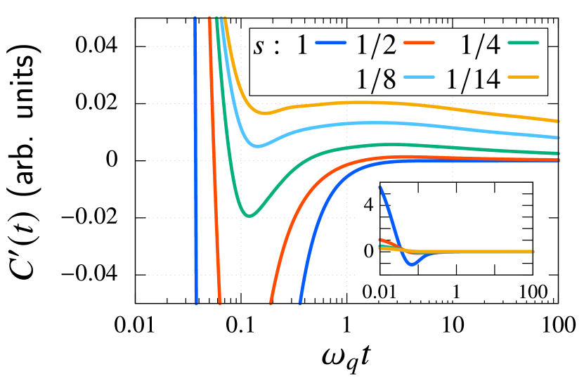
Figure 12: Real part of the two-time correlation function of the reservoir, $C^{\prime}(t)$, with arbitrary (arb.) units. Only the region around $0$, i.e., $-0.05\leq C^{\prime}(t)\leq 0.05$, is plotted to depict the detailed profile. The whole profile is exhibited in the inset.

Appendix C Two-time correlation function and depth of HEOM

Table 2: The number of modes for the two-time correlation function $K$ and the maximum depth of the hierarchy $\mathcal{N}_{\max}$ for various spectral exponents $s$. For the number in the parentheses, see Appendix C.

$s$	$1$	$1/2$	$1/4$	$1/8$	$1/14$
$K$	$10$	$24$	$18$	$8$ ($31$)	$7$ ($29$)
$\mathcal{N}_{\max}$	$3$	$3$	$4$	$8$	$10$

Here, we depict the two-time correlation function of the reservoir. The spectral density is given by Eq. (21), and the parameter values are the same as in the main text. The corresponding two-time correlation function is evaluated as Eq. (18) with the aid of the barycentric representation. The number of modes for the two-time correlation function $K$ is listed in Table 2. Figure 12 displays the dynamics of the real part of the two-time correlation function, $C^{\prime}(t)$. In the Ohmic case, the fast decay due to the large portion of the high frequency modes $\omega\simeq\omega_{c}$ is observed in the short-time region, $\omega_{q}t\leq 0.1$ (inset of Fig. 12), and the function approaches $0$ around the time $\omega_{q}t\simeq 5$. In the sub-Ohmic case, the fast decay in the short-time region is suppressed. As the spectral exponent decreases, slower decay in the long-time region is observed. In the case with $s\leq 1/4$, the correlation function takes a finite value even at the time $\omega_{q}t=100$. This slow decay results from the low frequency modes of the spectral noise power, which is approximated with $1/\omega^{1-s}$. As discussed in the main text, the slow decay causes non-Markovian effects, and the pure dephasing caused by this slow dynamics can be recovered with the Hahn-echo and dynamical-decoupling techniques.

As implied by the form of the influence functional in Eq. (66), the sluggish decay of $C(t)$ allows the system and reservoir to interact many times. Within the framework of HEOM, the depth of the hierarchy $\mathcal{N}_{\max}$ needs to be large in order to describe these multiple interactions. For this reason, $\mathcal{N}_{\max}$ increases as the spectral exponent $s$ decreases in Table  2. Note that since the multiple interactions cannot be described within the second-order perturbation theory, higher-order terms must be taken into account when one considers $1/f$-type noise with perturbative methods, e.g., time-convolutionless master equations.

Technically, simulations with lager $\mathcal{N}_{\max}$ demand more computational resources, and the cost for the simulations for $s=1/8$ and $1/14$ is prohibitively expensive. For this reason, we reduced the number of the elements $K$ with the aid of the method of least squares in those cases. The time evolution of the system subject to the phase errors is described only with the RDO ($\mathcal{N}_{\max}=0$), and the computational cost is less expensive. Therefore, we adopted the original sets $\{z_{k}\}$ and $\{d_{k}\}$ in this case instead of the approximate ones. The values of $K$ for $s=1/8$ and $1/14$ in Table 2 indicate the number of modes of the approximate set, while the number in parentheses is that of the original set.

Appendix D Dynamics of a single qubit without pulses

In this appendix, we investigate dynamics of a single qubit without pulses. We consider the same Hamiltonian as in the main text [Eq. (58)], with the amplitude $\Omega=0$. The parameter values of the spectral density are also the same as in the main text, and we used the HEOM to obtain the results.

D.1 Bit-flip error

D.1.1 Population relaxation

Here, we consider the bit-flip error, where the system part of the interaction Hamiltonian is given by $\hat{V}=\hbar\hat{\sigma}_{x}$, and focus on the dynamics of the population relaxation. The excited state $\hat{\rho}_{e}$ is chosen as the initial state. Figure 13 displays the dynamics of the expectation value $\expectationvalue*{\hat{\sigma}_{z}(t)}/2$ with the Ohmic and sub-Ohmic spectral densities. In the sub-Ohmic cases, we consider four exponents, $s=1/2$, $1/4$, $1/8$ and $1/14$, in the same way as the main text. As is clear from the inset of Fig. 13, the system reaches the equilibrium state up to the time $\omega_{q}t\leq 200$. We adopted the RDO and ADOs at the time $\omega_{q}t=200$ as the equilibrium initial states, $\hat{\rho}_{eq}$, which were used in the simulations of the pulse sequences in the main text.

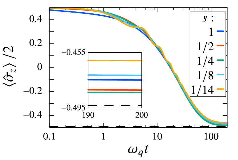
Figure 13: Dynamics of the expectation value $\expectationvalue*{\hat{\sigma}_{z}(t)}/2$ with various spectral densities. We do not consider pulses, which corresponds to $\Omega=0$, and the excited initial state is adopted ($\hat{\rho}_{0}=\hat{\rho}_{e}$). The dashed horizontal line indicates the value $\expectationvalue*{\hat{\sigma}_{z}(t)}/2=-0.5\tanh(\beta\hbar\omega_{q}/2)$, which corresponds to the equilibrium value obtained from the Boltzmann distribution of the bare system. The inset displays the expectation value in the long-time region.

Overall, the dynamics of the population relaxation is qualitatively similar irrespective of the spectral exponent $s$. This is because we chose the parameter values such that $S_{\beta}(\pm\omega_{q})$, which corresponds to the decay rate within the Bloch–Redfield theory [cf. Eq. (LABEL:eq:Lindblad)], takes the same value regardless of $s$. Conversely, the discrepancy of these dynamics indicates the effects beyond the Born–Markov approximation.

First, we focus on the dynamics in the short-time region, $\omega_{q}t\ll 1$. The slower decay is observed as the spectral exponent decreases, which results from the “universal decoherence” [22, 57] as follows: In the short-time region, the contribution of the system Hamiltonian $\hat{H}_{S}$ to the dynamics is negligibly small. Because we assume the condition $\hat{H}_{S}\simeq 0$, the commutation relation $[\hat{H}_{S},\hat{V}]=0$ holds. On the basis of this relation, we can apply the equations discussed in Appendix B.2. Note that because we consider the operator $\hat{V}=\hbar\hat{\sigma}_{x}$ here, the eigenstates in Appendix B.2 are no longer the ground and excited states, but the eigenstates of $\hat{\sigma}_{x}$, which is expressed as $(\ket{0}\pm\ket{1})/\sqrt{2}$. This change of the eigenstates leads to the correspondence of the decay rate of the decoherence expressed in Eq. (LABEL:eq:FID2) to that of the population relaxation in this case. The time evolution of the expectation value in the short-time region is evaluated as

$$\expectationvalue*{\hat{\sigma}_{z}(t)}= \exp\left[-4\hbar\int_{0}^{\infty}d\omega J(\omega)\coth\frac{\beta\hbar\omega}{2}\frac{1-\cos\omega t}{\omega^{2}}\right]\,.$$ (139)

Here, the initial state $\hat{\rho}_{e}$ is considered. This decay in the short-time region is referred to as the universal decoherence. When we consider further shorter-time region, $\omega_{c}t\ll 1$, we can approximate the term $(1-\cos\omega t)/\omega^{2}$ with $t^{2}/2$, and the decay rate is proportional to $J(\omega)\coth(\beta\hbar\omega/2)$. We confirmed that the area decreases as the spectral exponent decreases. Although the region $0.1<\omega_{q}t<1$ in Fig. 13 does not fulfill the condition $\omega_{c}t\ll 1$, which corresponds to the condition $\omega_{q}t\ll 0.02$ in our case, we found the similar tendency of the decay in this region: the decay is slower as the exponent decreases.

After the universal decoherence, relatively fast decay is observed around the time $\omega_{q}t\simeq 3$ for the deep sub-Ohmic reservoirs. The subsequent oscillatory behavior is found in the cases for $s=1/8$ and $1/14$. These oscillations are caused by the slow dynamics of the two-time correlation function of the reservoir and reflects the non-Markovianity of the reservoir.

Now, we turn to the analysis of the equilibrium states, the inset of Fig. 13. The dashed line in Fig. 13 is the expectation value for the equilibrium state obtained from the Born–Markov approach [$\expectationvalue*{\hat{\sigma}_{z}(t)}/2=-0.5\tanh(\beta\hbar\omega_{q}/2)$], and every result deviates from this. The system–reservoir coupling is ignored for the equilibrium states within the Born–Markov approximation, while included for the total equilibrium states. This difference leads to the deviation, which is smallest in the case for $s=1/4$, while largest in the case for $s=1/14$.

D.1.2 Ramsey experiments

In this section, we illustrate the numerical results of the Ramsey experiments. The initial state is given by $\hat{\rho}_{\mathrm{tot}}(0)=(\ket{0}+\ket{1})(\bra{0}+\bra{1})/2\otimes\hat{\rho}_{R,eq}$. Note that the Ramsey experiments discussed in Sec. VI are different from the experiment in this appendix, because the phase errors $\hat{V}=\hbar\hat{\sigma}_{z}$ were considered there while we here consider the bit-flip errors, $\hat{V}=\hbar\hat{\sigma}_{x}$.

We depict the time evolution of the Bloch vectors projected onto the $\expectationvalue*{\tilde{\sigma}_{x}}$–$\expectationvalue*{\tilde{\sigma}_{y}}$ plane in Fig 14. The initial state corresponds to the point $(0.5,0)$. Decoherence occurs during the time evolution, and the system reaches the equilibrium state, in which the off-diagonal elements are zero, corresponding to the point $(0,0)$. Here, the rotating frame $\hat{R}_{z}(-\omega_{q}t)\hat{\rho}_{S}(t)\hat{R}_{z}(\omega_{q}t)$ is considered. If the off-diagonal elements, $\expectationvalue*{\hat{\sigma}_{x}}$ and $\expectationvalue*{\hat{\sigma}_{y}}$, oscillate with the frequency $\omega_{q}$, the projected Bloch vector in the rotating frame is always in the direction of $\expectationvalue*{\tilde{\sigma}_{x}}$. In the Bloch–Redfield theory, the frequency change from $\omega_{q}$ due to the Lamb shift, and the projected Bloch vector rotates. Because the Lamb shift is time-independent within this approximation and the length of the vector decreases due to the relaxation, the locus is a spiral. In our case, however, the oscillatory behavior along the spiral is observed. This implies that we cannot express the oscillation behavior with a single frequency.

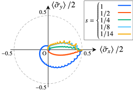
Figure 14: Time evolution of the Bloch vectors projected onto the $\expectationvalue*{\tilde{\sigma}_{x}}$–$\expectationvalue*{\tilde{\sigma}_{y}}$ plane.

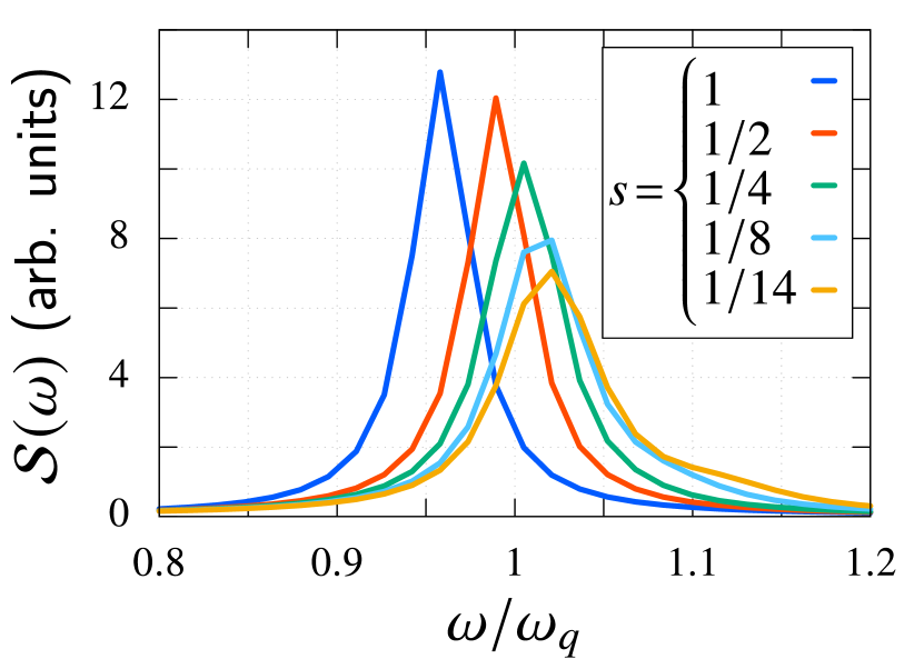
Figure 15: Fourier transform of $\expectationvalue*{\hat{\sigma}_{x}(t)}$ obtained with the Ramsey experiments, $\mathcal{S}(\omega)$, with arbitrary (arb.) units. The bit-flip error $\hat{V}=\hbar\hat{\sigma}_{x}$ is considered.

Figure 15 displays the Fourier transform of $\expectationvalue*{\hat{\sigma}_{x}(t)}$ obtained with the Ramsey experiments, which is defined as

$$\mathcal{S}(\omega)=\mathrm{Re}\left\{\int_{0}^{\infty}dt\frac{\expectationvalue*{\hat{\sigma}_{x}(t)}}{2}e^{-i\omega t}\right\}\,.$$ (140)

The upper bound of the integral is replaced with a sufficiently large value ($t=400/\omega_{q}$ in this case). The effective frequency of the qubit increases as the spectral exponent decreases. It is smaller than $\omega_{q}$ in the cases $s=1$ and $1/2$, while larger in the cases $s=1/4$, $1/8$ and $1/14$. This corresponds to the direction of the rotation of the spiral in Fig. 14. In addition, the absolute value of the frequency shift reflects the degree of the deviation of the locus from the $\expectationvalue*{\tilde{\sigma}_{x}}$ axis. As discussed above, even if we choose the effective frequency obtained in Fig. 15 for $\omega_{\mathrm{ex}}$, the oscillatory behavior cannot be removed completely.

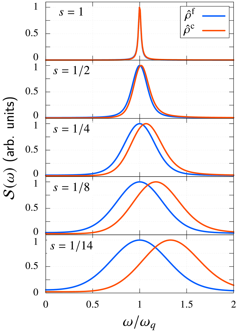
Figure 16: Fourier transform of $\expectationvalue*{\hat{\sigma}_{x}(t)}$ obtained with the Ramsey experiments, $\mathcal{S}(\omega)$, with arbitrary (arb.) units. Each curve is normalized such that the maximum value is $1$. The results with the factorized ($\hat{\rho}^{\mathrm{f}}$, blue curve) and correlated ($\hat{\rho}^{\mathrm{c}}$, red curve) initial state are depicted.

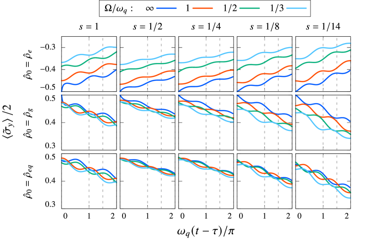
Figure 17: Dynamics of the expectation value $\expectationvalue*{\tilde{\sigma}_{y}(t)}/2$ in the rotating frame during the first idle phase with various initial states $\hat{\rho}_{0}$ and spectral exponents $s$. The sequence of $R_{x}(\pi/2)$ gates is considered. The gray vertical dashed lines indicate $\Delta t$ in Fig. 6.

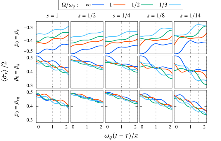
Figure 18: Dynamics of the expectation value $\expectationvalue*{\tilde{\sigma}_{x}(t)}/2$ in the rotating frame during the first idle phase with various initial states $\hat{\rho}_{0}$ and spectral exponents $s$. The sequence of three $H$ gates is applied. The gray vertical dashed lines indicate $\Delta t$ in Fig. 7.

D.2 Phase error: Ramsey experiments

In this section, we consider the phase error, $\hat{V}=\hbar\hat{\sigma}_{z}$. Because $\hat{H}_{S}$ and $\hat{V}$ commute, only the decoherence of the off-diagonal element is observed, and the relaxation process of the population does not occur. For this reason, we here focus on the Ramsey experiments, especially the difference between the factorized and correlated initial state.

We depict the Fourier transform of $\expectationvalue*{\hat{\sigma}_{x}(t)}$ obtained with the Ramsey experiments [Eq. (140)] in Fig 16. The results with the factorized [Eq. (LABEL:eq:FID2)] and correlated [Eq. (133)] initial state are displayed. For the factorized initial state, the reservoir does not change the Larmor frequency, as indicated by Eq. (LABEL:eq:FID2), and the peak of each blue curve is found at $\omega=\omega_{q}$ in Fig. 16. By contrast, the effective Larmor frequency is modified with the term $i\int dt^{\prime}\bar{L}(t^{\prime})$ in Eq. (133) in the case with the correlated initial state. Because we consider the low temperature $\beta\hbar\omega_{q}=5$, the contribution of $\rho_{-}(t)$ to $\rho_{eg}(t)$ in Eq. (130) is small. The frequency of $\rho_{+}(t)$ at the time $t$ is given by $\omega_{q}+4\int_{0}^{t}dt^{\prime}\bar{L}(t^{\prime})$ in Eq. (133), and we found that the function $\bar{L}(t)$ always takes nonnegative value in our simulations. For this reason, the peak for the correlated initial state is shifted to a larger frequency, which is indicated by the red curves in Fig. 16. The function $\bar{L}(t)$ decays slower as the spectral exponent $s$ decreases, and hence the integral of $\bar{L}(t)$ takes larger values. This results in the larger shift of the red curve in Fig. 16 for the smaller exponent.

The negligible contribution of $\rho_{-}(t)$ also leads to the correspondence of the absolute value $|\rho_{eg}(t)|$ between the factorized and correlated initial state, as discussed in Sec. VI. The absolute value is well approximated as $|\rho_{eg}(t)|\simeq|\rho_{+}(t)|$ at the low temperature, and the term $i\int dt^{\prime}\bar{L}(t^{\prime})$ does not affect the absolute value under this approximation.

Appendix E Detailed dynamics of a qubit during idle phases

In Sec. IV.1, dynamics of the first idle phase after the $R_{x}(\pi)$-gate application were discussed (Fig. 3). Here, we report other interesting dynamics during idle phases.

E.1 $R_{x}(\pi/2)$ gates

Figure 17 displays dynamics of the $\expectationvalue*{\tilde{\sigma}_{y}}$ element of the Bloch vector during the first idle phase of the $R_{x}(\pi/2)$-gate sequence. In contrast to the case of the $R_{x}(\pi)$ gates (Fig. 3), the oscillatory behavior is universally observed. It is found that this oscillation has a $\pi$-periodicity with respect to $\omega_{q}\tau$ [$=\pi\omega_{q}/(2\Omega)$]. The relative angle of $\hat{V}\propto\hat{\sigma}_{x}$ and $\tilde{\sigma}_{y}$ determines this periodicity. The fast decoherence around the time $t\simeq\tau$ is observed with $\Omega=\infty$ for the reservoir $s=1$, which is gradually suppressed as the spectral exponent decreases. High frequency modes of the spectral density cause steep decay of both population and coherence. The amplitude of the oscillation tends to be smallest for $s=1/2$ and $1/4$, while largest for $s=1$ and $1/14$. This reflects the effective Larmor frequency obtained from Fig. 15 and appears to be related to the tendency of the fidelity in terms of $s$ discussed in the main text.

The peculiar oscillation, which was found in the $R_{x}(\pi)$-gate cases (Sec. IV.1), is not observed in Fig. 17. This leads to the emergence of the expected order in all the cases in Fig. 6(a)–6(c) at $d=2$.

The time $t=\tau$ corresponds to the end of the first pulse application, $d=1$. The absolute value $|\expectationvalue*{\tilde{\sigma}_{y}}|$ mainly contributes to the fidelity and is in general smaller with the initial state $\hat{\rho}_{e}$ than with the state $\hat{\rho}_{g}$ and $\hat{\rho}_{eq}$ for a fixed $\Omega$. As discussed in the main text, the rotation from $(0,0,1)$ to $(0,-1,0)$ is disadvantageous compared to the rotation from $(0,0,-1)$ to $(0,1,0)$.

E.2 Hadamard ($H$) gates

Dynamics of the $\expectationvalue*{\tilde{\sigma}_{x}}$ element of the Bloch vector during the first idle phase of the $H$-gate sequence are depicted in Fig 18. In the cases for $s\leq 1/4$ with $\hat{\rho}_{0}=\hat{\rho}_{e}$ and $\hat{\rho}_{g}$, periodical oscillations are no longer observed, while oscillatory behavior similar to the $R_{x}(\pi/2)$-gate case is observed in the other cases. For the non-periodical results, one finds intense decay of the expectation value around the time $\omega_{q}(t-\tau)/\pi\simeq 0.5$ with the amplitude $\Omega/\omega_{q}=\infty$ and $1$, while $\omega_{q}(t-\tau)/\pi\simeq 1.5$ with $\Omega/\omega_{q}=1/2$ and $1/3$, which leads to the violation of the expected order defined in the main text. The slow decay of the two-time correlation function appears to contribute to this behavior. It is also enhanced in the instantaneous-pulse case: the slow re-establishment of the system–reservoir correlations contributes. This argument is also supported by the fact that this behavior is suppressed in the case $\hat{\rho}_{0}=\hat{\rho}_{eq}$.

The initial phase of the oscillation behavior is different with $\pi$ from the case of $R_{x}(\pi/2)$ gates, and the fast decoherence around the time $t=\tau$ with $\Omega=\infty$ for $s=1$ is not observed due to this difference of the initial phase.

In the same manner as the $R_{x}(\pi/2)$ gates, the absolute value $|\expectationvalue*{\tilde{\sigma}_{x}}|$ mainly contributes to the fidelity, and it is worse in case $\hat{\rho}_{e}$ than in the other two cases. The disadvantage of the $\pi/2$-rotation from the excited state is independent of the rotation axis.

E.3 Asymptotic behavior with respect to the pulse duration

Figure 19 displays the dynamics of the $\expectationvalue*{\hat{\sigma}_{z}}$ element of the Bloch vector during the second idle phase of the $R_{x}(\pi)$-gate sequence. The cases with $\hat{\rho}_{0}=\hat{\rho}_{g}$ and $\hat{\rho}_{eq}$ for $s=1$ and $1/14$ are depicted as representatives. We varied the amplitudes and durations of the idle phase, as $\Omega/\omega_{q}=1$ and $1/3$ [(a) and (b) in each panel], and $\omega_{q}\Delta t/\pi=1$, $3/2$, and $2$, respectively.

The decay is nearly linear irrespective of $\Delta t$ in the Ohmic case ($s=1$, left panel), and further, the rate is almost independent of $\Delta t$, while similar behavior is only observed in the deep sub-Ohmic case ($s=1/14$, right panel) with the condition $\Omega/\omega_{q}=1/3$ and $\hat{\rho}_{0}=\hat{\rho}_{eq}$. This indicates that when the pulse duration is sufficiently large and the initial state is prepared into the equilibrium state, the decay with an almost same rate irrespective of $\Delta t$ and $s$ occurs. From this result, we can interpret this behavior as asymptotic behavior with respect to the pulse duration. As discussed above, the reconfiguration process is less significant with the initial state $\hat{\rho}_{0}=\hat{\rho}_{eq}$ compared to $\hat{\rho}_{e}$ and $\hat{\rho}_{g}$. In addition, the process is completed in a shorter period of time when the decay of the two-time correlation function is faster. We found that the asymptotic behavior tends to be observed in the cases where the impact of the reconfiguration is small, and we suggest that the Markovianity of the reservoir contributes to this asymptotic behavior.

Note that during a sequence with the impulsive pulses, the above asymptotic behavior is not observed even in the Ohmic case. The reconfiguration process does not occur during the pulse application, and hence the dynamics during the second idle phase are directly affected by those during the first idle phase.

Finally, we comprehensively mention the behavior during the second idle phase. In the case for $s\geq 1/2$, the asymptotic behavior is always observed for the pulse amplitude $\Omega/\omega_{q}=1$, $1/2$ and $1/3$, with the initial state $\hat{\rho}_{0}=\hat{\rho}_{e}$, $\hat{\rho}_{g}$ and $\hat{\rho}_{eq}$, while in the case for $s\leq 1/8$, this behavior is only observed for $\Omega/\omega_{q}=1/3$ with $\hat{\rho}_{0}=\hat{\rho}_{eq}$. The case for $s=1/4$ is intermediate of these two cases: the asymptotic behavior is observed for $\Omega/\omega_{q}=1/3$ with all the initial states.

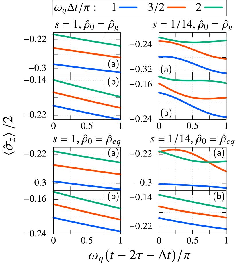
Figure 19: Dynamics of the expectation value $\expectationvalue*{\hat{\sigma}_{z}(t)}/2$ during the second idle phase of the sequence of three $R_{x}(\pi)$ gates. As representatives, the cases for $s=1$ and $s=1/14$ are depicted. The initial states are given by $\hat{\rho}_{0}=\hat{\rho}_{g}$ and $\hat{\rho}_{eq}$, respectively. The pulse amplitude is chosen as follows: (a) $\Omega/\omega_{q}=1$, (b) $\Omega/\omega_{q}=1/3$.

Appendix F Time constants for the Ramsey, echo and dynamical-decoupling experiments

In this appendix we explain the fitting methods to obtain the time constants in Sec. VI. We conducted the method of least squares and evaluated the time constants $T_{\mathrm{R}}$, $T_{\mathrm{E}}$ and $T_{\mathrm{DD}}$. In the Ramsey experiments for $s=1$ and $1/2$, fast decay of $|\rho_{eg}(t)|$ was observed. Therefore, we considered the following functions as model curves;

$$|\bar{\rho}_{eg}(t)|_{(1)} =A\exp\left[-Bt\right]+C\exp\left[-Dt\right]+E\,,$$ (141)

$$|\bar{\rho}_{eg}(t)|_{(2)} =A\exp\left[-Bt\right]+C\exp\left[-(Dt)^{2}\right]+E\,,\quad$$ (142)

and compared the residuals of the method of least squares. In the case for $s=1$, a smaller residual was obtained with the curve Eq. (141) compared to the curve Eq. (142), while the opposite result was obtained in the case $s=1/2$. In both cases, $T_{\mathrm{R}}$ was evaluated with the relation $T_{\mathrm{R}}=1/D$. Here, we have defined $D<B$ in the Ohmic case, and we found the relation $D<B$ in the case $s=1/2$.

In the other cases of the Ramsey experiments, the cases of the HE experiments with the condition $s\neq 1$, and all the cases of the DD experiments, fast decay was not observed, and we considered an exponential function,

$$|\bar{\rho}_{eg}(t)|_{(3)}=a\exp\left[-bt\right]+c\,,$$ (143)

and a Gaussian function,

$$|\bar{\rho}_{eg}(t)|_{(4)}=a\exp\left[-(bt)^{2}\right]+c$$ (144)

as model curves. In the Ramsey cases for $s\leq 1/4$ and the HE cases for $s\neq 1$, we found that the Gaussian fitting was better than the exponential fitting. For the DD experiments, we obtained better results with the exponential fitting compared to the Gaussian fitting.

For the HE experiment for $s=1$, we evaluated the time constant from the asymptotic behavior of $|\rho_{eg}(t)|$: we found from Fig. 10(c) that the dynamics after the fast decay with different $\Delta t$ can be represented by a single curve. We used this curve for the evaluation. The model curve $|\bar{\rho}_{eg}(t)|_{(3)}$ and $|\bar{\rho}_{eg}(t)|_{(4)}$ were considered, and the exponential fitting was found to be better. The time constants obtained with these curves are listed and plotted in Table 1 and Fig. 11(d).

References

- Place et al. [2021] A. P. M. Place, L. V. H. Rodgers, P. Mundada, B. M. Smitham, M. Fitzpatrick, Z. Leng, A. Premkumar, J. Bryon, A. Vrajitoarea, S. Sussman, et al., New material platform for superconducting transmon qubits with coherence times exceeding 0.3 milliseconds, Nat. Commun. 12, 1779 (2021).
- Wang et al. [2022] C. Wang, X. Li, H. Xu, Z. Li, J. Wang, Z. Yang, Z. Mi, X. Liang, T. Su, C. Yang, et al., Towards practical quantum computers: transmon qubit with a lifetime approaching 0.5 milliseconds, npj Quantum Inf. 8, 3 (2022).
- Negîrneac et al. [2021] V. Negîrneac, H. Ali, N. Muthusubramanian, F. Battistel, R. Sagastizabal, M. S. Moreira, J. F. Marques, W. J. Vlothuizen, M. Beekman, C. Zachariadis, et al., High-Fidelity Controlled- Gate with Maximal Intermediate Leakage Operating at the Speed Limit in a Superconducting Quantum Processor, Phys. Rev. Lett. 126, 220502 (2021).
- Sung et al. [2021] Y. Sung, L. Ding, J. Braumüller, A. Vepsäläinen, B. Kannan, M. Kjaergaard, A. Greene, G. O. Samach, C. McNally, D. Kim, et al., Realization of High-Fidelity CZ and -Free iSWAP Gates with a Tunable Coupler, Phys. Rev. X 11, 021058 (2021).
- Kandala et al. [2021] A. Kandala, K. X. Wei, S. Srinivasan, E. Magesan, S. Carnevale, G. A. Keefe, D. Klaus, O. Dial, and D. C. McKay, Demonstration of a High-Fidelity cnot Gate for Fixed-Frequency Transmons with Engineered Suppression, Phys. Rev. Lett. 127, 130501 (2021).
- Arute et al. [2019] F. Arute, K. Arya, R. Babbush, D. Bacon, J. C. Bardin, R. Barends, R. Biswas, S. Boixo, F. G. S. L. Brandao, D. A. Buell, et al., Quantum supremacy using a programmable superconducting processor, Nature (London) 574, 505 (2019).
- Google Quantum AI [2023] Google Quantum AI, Suppressing quantum errors by scaling a surface code logical qubit, Nature (London) 614, 676 (2023).
- Kim et al. [2023] Y. Kim, A. Eddins, S. Anand, K. X. Wei, E. van den Berg, S. Rosenblatt, H. Nayfeh, Y. Wu, M. Zaletel, K. Temme, et al., Evidence for the utility of quantum computing before fault tolerance, Nature (London) 618, 500 (2023).
- Havlíček et al. [2019] V. Havlíček, A. D. Córcoles, K. Temme, A. W. Harrow, A. Kandala, J. M. Chow, and J. M. Gambetta, Supervised learning with quantum-enhanced feature spaces, Nature (London) 567, 209 (2019).
- Kandala et al. [2017] A. Kandala, A. Mezzacapo, K. Temme, M. Takita, M. Brink, J. M. Chow, and J. M. Gambetta, Hardware-efficient variational quantum eigensolver for small molecules and quantum magnets, Nature (London) 549, 242 (2017).
- Rossmannek et al. [2023] M. Rossmannek, F. Pavošević, A. Rubio, and I. Tavernelli, Quantum Embedding Method for the Simulation of Strongly Correlated Systems on Quantum Computers, J. Phys. Chem. Lett. 14, 3491 (2023).
- Willsch et al. [2020] M. Willsch, D. Willsch, F. Jin, H. De Raedt, and K. Michielsen, Benchmarking the quantum approximate optimization algorithm, Quantum Inf. Process. 19, 197 (2020).
- García-Pérez et al. [2020] G. García-Pérez, M. A. C. Rossi, and S. Maniscalco, IBM Q Experience as a versatile experimental testbed for simulating open quantum systems, npj Quantum Inf. 6, 1 (2020).
- [14] R. C. Farrell, M. Illa, A. N. Ciavarella, and M. J. Savage, Quantum Simulations of Hadron Dynamics in the Schwinger Model using 112 Qubits, arXiv:2401.08044 [quant-ph] .
- Devitt et al. [2013] S. J. Devitt, W. J. Munro, and K. Nemoto, Quantum error correction for beginners, Rep. Prog. Phys. 76, 076001 (2013).
- Cai et al. [2023] Z. Cai, R. Babbush, S. C. Benjamin, S. Endo, W. J. Huggins, Y. Li, J. R. McClean, and T. E. O’Brien, Quantum error mitigation, Rev. Mod. Phys. 95, 045005 (2023).
- Gulácsi and Burkard [2023] B. Gulácsi and G. Burkard, Signatures of non-Markovianity of a superconducting qubit, Phys. Rev. B 107, 174511 (2023).
- [18] M. Papič, A. Auer, and I. de Vega, Fast Estimation of Physical Error Contributions of Quantum Gates, arXiv:2305.08916 [quant-ph] .
- Ristè et al. [2013] D. Ristè, C. C. Bultink, M. J. Tiggelman, R. N. Schouten, K. W. Lehnert, and L. DiCarlo, Millisecond charge-parity fluctuations and induced decoherence in a superconducting transmon qubit, Nat. Commun. 4, 1913 (2013).
- Cardani et al. [2021] L. Cardani, F. Valenti, N. Casali, G. Catelani, T. Charpentier, M. Clemenza, I. Colantoni, A. Cruciani, G. D’Imperio, L. Gironi, et al., Reducing the impact of radioactivity on quantum circuits in a deep-underground facility, Nat. Commun. 12, 2733 (2021).
- Pan et al. [2022] X. Pan, Y. Zhou, H. Yuan, L. Nie, W. Wei, L. Zhang, J. Li, S. Liu, Z. H. Jiang, G. Catelani, et al., Engineering superconducting qubits to reduce quasiparticles and charge noise, Nat. Commun. 13, 7196 (2022).
- Tuorila et al. [2019] J. Tuorila, J. Stockburger, T. Ala-Nissila, J. Ankerhold, and M. Möttönen, System-environment correlations in qubit initialization and control, Phys. Rev. Res. 1, 013004 (2019).
- Babu et al. [2021] A. P. Babu, J. Tuorila, and T. Ala-Nissila, State leakage during fast decay and control of a superconducting transmon qubit, npj Quantum Inf. 7, 30 (2021).
- Nakamura and Ankerhold [2024] K. Nakamura and J. Ankerhold, Qubit dynamics beyond Lindblad: Non-Markovianity versus rotating wave approximation, Phys. Rev. B 109, 014315 (2024).
- Babu et al. [2023] A. P. Babu, T. Orell, V. Vadimov, W. Teixeira, M. Möttönen, and M. Silveri, Quantum error correction under numerically exact open-quantum-system dynamics, Phys. Rev. Res. 5, 043161 (2023).
- [26] P. Figueroa-Romero, M. Papič, A. Auer, M.-H. Hsieh, K. Modi, and I. de Vega, Operational Markovianization in Randomized Benchmarking, arXiv:2305.04704 [quant-ph] .
- [27] A. Agarwal, L. P. Lindoy, D. Lall, F. Jamet, and I. Rungger, Modelling non-Markovian noise in driven superconducting qubits, arXiv:2306.13021 [quant-ph] .
- Xu et al. [2022] M. Xu, Y. Yan, Q. Shi, J. Ankerhold, and J. T. Stockburger, Taming Quantum Noise for Efficient Low Temperature Simulations of Open Quantum Systems, Phys. Rev. Lett. 129, 230601 (2022).
- Blais et al. [2021] A. Blais, A. L. Grimsmo, S. M. Girvin, and A. Wallraff, Circuit quantum electrodynamics, Rev. Mod. Phys. 93, 025005 (2021).
- Breuer and Petruccione [2002] H.-P. Breuer and F. Petruccione, The theory of Open Quantum Systems (Oxford University Press, Oxford, 2002).
- Weiss [2012] U. Weiss, Quantum Dissipative Systems, 4th ed. (World Scientific, Singapore, 2012).
- Ithier et al. [2005] G. Ithier, E. Collin, P. Joyez, P. J. Meeson, D. Vion, D. Esteve, F. Chiarello, A. Shnirman, Y. Makhlin, J. Schriefl, et al., Decoherence in a superconducting quantum bit circuit, Phys. Rev. B 72, 134519 (2005).
- Tanimura [2015] Y. Tanimura, Real-time and imaginary-time quantum hierarchal Fokker–Planck equations, J. Chem. Phys. 142, 144110 (2015).
- Tanimura [2020] Y. Tanimura, Numerically “exact” approach to open quantum dynamics: The hierarchical equations of motion (HEOM), J. Chem. Phys. 153, 020901 (2020).
- [35] M. Xu, V. Vadimov, M. Krug, J. T. Stockburger, and J. Ankerhold, A Universal Framework for Quantum Dissipation:Minimally Extended State Space and Exact Time-Local Dynamics, arXiv:2307.16790 [quant-ph] .
- Bylander et al. [2011] J. Bylander, S. Gustavsson, F. Yan, F. Yoshihara, K. Harrabi, G. Fitch, D. G. Cory, Y. Nakamura, J.-S. Tsai, and W. D. Oliver, Noise spectroscopy through dynamical decoupling with a superconducting flux qubit, Nat. Phys. 7, 565 (2011).
- Barone and Paternò [1982] A. Barone and G. Paternò, Physics and Applications of the Josephson Effect (John Wiley & Sons, New York, 1982).
- [38] G. Wendin and V. S. Shumeiko, Superconducting Quantum Circuits, Qubits and Computing, arXiv:cond-mat/0508729 [cond-mat.supr-con] .
- Machlup [1954] S. Machlup, Noise in Semiconductors: Spectrum of a Two‐Parameter Random Signal, J. Appl. Phys. 25, 341 (1954).
- Paladino et al. [2014] E. Paladino, Y. M. Galperin, G. Falci, and B. L. Altshuler, noise: Implications for solid-state quantum information, Rev. Mod. Phys. 86, 361 (2014).
- Müller et al. [2019] C. Müller, J. H. Cole, and J. Lisenfeld, Towards understanding two-level-systems in amorphous solids: insights from quantum circuits, Rep. Prog. Phys. 82, 124501 (2019).
- Glazman and Catelani [2021] L. I. Glazman and G. Catelani, Bogoliubov quasiparticles in superconducting qubits, SciPost Phys. Lect. Notes , 31 (2021).
- Eroms et al. [2006] J. Eroms, L. C. van Schaarenburg, E. F. C. Driessen, J. H. Plantenberg, C. M. Huizinga, R. N. Schouten, A. H. Verbruggen, C. J. P. M. Harmans, and J. E. Mooij, Low-frequency noise in Josephson junctions for superconducting qubits, Appl. Phys. Lett. 89, 122516 (2006).
- Nugroho et al. [2013] C. D. Nugroho, V. Orlyanchik, and D. J. Van Harlingen, Low frequency resistance and critical current fluctuations in Al-based Josephson junctions, Appl. Phys. Lett. 102, 142602 (2013).
- Kenyon et al. [2000] M. Kenyon, C. J. Lobb, and F. C. Wellstood, Temperature dependence of low-frequency noise in Al–Al2O3–Al single-electron transistors, J. Appl. Phys. 88, 6536 (2000).
- Wellstood et al. [2004] F. C. Wellstood, C. Urbina, and J. Clarke, Flicker () noise in the critical current of Josephson junctions at –K, Appl. Phys. Lett. 85, 5296 (2004).
- Tanimura [2014] Y. Tanimura, Reduced hierarchical equations of motion in real and imaginary time: Correlated initial states and thermodynamic quantities, J. Chem. Phys. 141, 044114 (2014).
- McKay et al. [2017] D. C. McKay, C. J. Wood, S. Sheldon, J. M. Chow, and J. M. Gambetta, Efficient gates for quantum computing, Phys. Rev. A 96, 022330 (2017).
- Alicki and Lendi [1987] R. Alicki and K. Lendi, Quantum Dynamical Semigroups and Applications (Springer-Verlag, Berlin, 1987).
- Rivas and Huelga [2012] Á. Rivas and S. F. Huelga, Open Quantum Systems: An Introduction (Springer, Heidelberg, 2012).
- Viola and Lloyd [1998] L. Viola and S. Lloyd, Dynamical suppression of decoherence in two-state quantum systems, Phys. Rev. A 58, 2733 (1998).
- Shiokawa and Lidar [2004] K. Shiokawa and D. A. Lidar, Dynamical decoupling using slow pulses: Efficient suppression of noise, Phys. Rev. A 69, 030302 (2004).
- Rego et al. [2009] L. G. Rego, L. F. Santos, and V. S. Batista, Coherent Control of Quantum Dynamics with Sequences of Unitary Phase-Kick Pulses, Annu. Rev. Phys. Chem. 60, 293 (2009).
- Carr and Purcell [1954] H. Y. Carr and E. M. Purcell, Effects of Diffusion on Free Precession in Nuclear Magnetic Resonance Experiments, Phys. Rev. 94, 630 (1954).
- Meiboom and Gill [1958] S. Meiboom and D. Gill, Modified Spin–Echo Method for Measuring Nuclear Relaxation Times, Rev. Sci. Instrum. 29, 688 (1958).
- Tanimura [2006] Y. Tanimura, Stochastic Liouville, Langevin, Fokker–Planck, and Master Equation Approaches to Quantum Dissipative Systems, J. Phys. Soc. Jpn. 75, 082001 (2006).
- Braun et al. [2001] D. Braun, F. Haake, and W. T. Strunz, Universality of Decoherence, Phys. Rev. Lett. 86, 2913 (2001).
- Motzoi et al. [2009] F. Motzoi, J. M. Gambetta, P. Rebentrost, and F. K. Wilhelm, Simple Pulses for Elimination of Leakage in Weakly Nonlinear Qubits, Phys. Rev. Lett. 103, 110501 (2009).
- Radcliffe [1971] J. M. Radcliffe, Some properties of coherent spin states, J. Phys. A 4, 313 (1971).
- Nakamura and Tanimura [2018] K. Nakamura and Y. Tanimura, Hierarchical Schrödinger equations of motion for open quantum dynamics, Phys. Rev. A 98, 012109 (2018).
- Ikeda and Scholes [2020] T. Ikeda and G. D. Scholes, Generalization of the hierarchical equations of motion theory for efficient calculations with arbitrary correlation functions, J. Chem. Phys. 152, 204101 (2020).
- Liniov et al. [2019] A. Liniov, I. Meyerov, E. Kozinov, V. Volokitin, I. Yusipov, M. Ivanchenko, and S. Denisov, Unfolding a quantum master equation into a system of real-valued equations: Computationally effective expansion over the basis of generators, Phys. Rev. E 100, 053305 (2019).
- Kubo et al. [1985] R. Kubo, M. Toda, and N. Hashitsume, Statistical Physics II Nonequilibrium Statistical Mechanics (Springer-Verlag, Berlin, 1985).