Log Neural Controlled Differential Equations:
The Lie Brackets Make a Difference
2Department of Electrical Engineering, City University of Hong Kong, Hong Kong
)
Abstract
The vector field of a controlled differential equation (CDE) describes the relationship between a control path and the evolution of a solution path. Neural CDEs (NCDEs) treat time series data as observations from a control path, parameterise a CDE’s vector field using a neural network, and use the solution path as a continuously evolving hidden state. As their formulation makes them robust to irregular sampling rates, NCDEs are a powerful approach for modelling real-world data. Building on neural rough differential equations (NRDEs), we introduce Log-NCDEs, a novel and effective method for training NCDEs. The core component of Log-NCDEs is the Log-ODE method, a tool from the study of rough paths for approximating a CDE’s solution. On a range of multivariate time series classification benchmarks, Log-NCDEs are shown to achieve a higher average test set accuracy than NCDEs, NRDEs, and two state-of-the-art models, S5 and the linear recurrent unit.
1 Introduction
1.1 Multivariate Time Series Modelling
Neural controlled differential equations (NCDEs) are a method for modelling multivariate time series, which offer a number of advantages for real-world applications. These include decoupling the number of forward passes through their neural network from the number of observations in the time series, as well as being robust to irregular sampling rates. However, there exists a gap in performance between NCDEs and current state-of-the-art approaches for time series modelling, such as S5 and the linear recurrent unit (LRU) [1, 2].
This paper demonstrates that, on a range of multivariate time series classification benchmarks, the gap in performance between NCDEs and other state-of-the-art approaches can be closed by utilising the Log-ODE method during training. We refer to this new approach as Log-NCDEs.
1.2 Neural Controlled Differential Equations
Let denote a set of observations from a multivariate time series, where . Let be a continuous interpolation, such that , where subscript on a time-dependent variables denotes evaluation. Let and be neural networks, and be a linear map. A NCDE is defined by
| (1) | ||||
for , where is matrix-vector multiplication [3]. Details on the regularity required for existence and uniqueness of the solution to (1) can be found in appendix A.2. A sufficient condition is being of bounded variation and being Lipschitz continuous [4].
NCDEs are an attractive option for modelling multivariate time series. They are universal approximators of continuous real-valued functions on time series data [5, Theorem 3.9]. Additionally, since they interact with time series data through the continuous interpolation , NCDEs are agnostic to when the data was sampled. This makes them robust to irregular sampling rates. Furthermore, the number of forward passes through when evaluating (1) is controlled by the differential equation solver used. This is opposed to recurrent models, where it is controlled by the number of observations . By decoupling the number of forward passes through their neural network from the number of observations in the time series, NCDEs can mitigate exploding or vanishing gradients on highly-sampled time series.
To make use of the techniques developed for training neural ordinary differential equations (ODEs) [6], NCDEs are typically rewritten as an ODE,
| (2) |
where . If is taken to be a differentiable interpolation, then a choice of is
| (3) |
1.3 Neural Rough Differential Equations
Neural rough differential equations (NRDEs) are based on the Log-ODE method, which is introduced briefly here. Detailed descriptions of regularity, the log-signature, and Lie brackets will be given in section 2.
Assume that satisfies a regularity constraint, , and let denote the depth- truncated log-signature of X over . Letting , a depth- Log-ODE method approximates the solution of (1) by using (2) with
| (4) |
for , where the depth and is constructed using the iterated Lie brackets of [7]. Note that when using (3), is exactly for all , whereas when using (4), is an approximation of when .
NRDEs use (4), but rather than being constructed from the iterated Lie brackets of , it is treated as a neural network , where is the dimension of a depth truncated log-signature of a dimensional path. By neglecting the structure of , NRDEs are able to reduce the computational cost of a forward pass through the network, at the cost of increasing the output dimension of the neural network.
Compared to NCDEs, NRDEs can reduce the number of forward passes through the network while evaluating the model, as the vector field is autonomous on each interval . This has been shown to lead to improved classification accuracy, alongside reduced time and memory-usage, on time series with up to 17,000 observations [8]. Furthermore, as it is no longer necessary to apply a differentiable interpolation to the time series data, NRDEs are applicable to a wider range of input signals.
1.4 Contributions
This paper introduces Log-NCDEs, which build on NRDEs by constructing using the iterated Lie brackets of a NCDE’s vector field, . This change significantly reduces the output dimension of the model’s neural network, while maintaining the same expressivity. Calculating the Lie brackets requires that, when applying a depth- Log-ODE method, be for . Section 3.2 presents a novel theoretical result bounding the norm for a class of fully connected neural networks when . Following this, section 3.3 details how to efficiently calculate the Lie bracket of a neural network using existing tools in machine learning. The paper concludes by showing that, over a range of multivariate time series classification benchmarks, Log-NCDEs achieve a higher average test set accuracy than NCDEs, NRDEs, S5, and LRU.
2 Mathematical Background
The vector field of a CDE is typically thought of as a matrix-valued function . An equivalent formulation is being a linear map acting on and returning a vector field on . In other words, . This formulation will prove more useful in the following section.
2.1 The Tensor Product
Definition 2.1.
Let , , and be vector spaces. The tensor product space is the unique (up to isomorphism) space such that for all bilinear functions there exists a unique linear map , such that [9].
As an example, let and . In this case, the tensor product is the outer product of the two vectors, and the resulting tensor product space is the space of matrices, . The tensor product of and is defined by
| (5) |
where any bilinear function can be written as a linear function .
Definition 2.2.
The tensor algebra space is the space
| (7) |
where .
2.2 Functions
is a notion of regularity for functions defined on closed sets. It is the regularity used in the statements of existence and uniqueness of solutions to CDEs and the regularity required for the Log-ODE method to be well defined.
A general definition of for functions on Banach spaces can be found in appendix A.1. This paper considers the regularity of vector fields on . In this case, for implies that is bounded, has bounded derivatives, and the derivative satisfies
| (8) |
for all .
2.3 Lie Brackets
Definition 2.3.
A Lie algebra is a vector space with a bilinear map satisfying and the Jacobi identity,
| (9) |
for all . The map is called the Lie bracket [10].
Any associative algebra, , has a Lie bracket structure with Lie bracket defined by
| (10) |
for all . For example, with the matrix product. For an example that does not arise from an associative algebra, let denote the set of all infinitely differentiable functions from to . When equipped with addition, is a vector space. Furthermore, is a Lie algebra when equipped with the Lie bracket
| (11) |
where is the Jacobian of with entries given by for .
Definition 2.4.
For a Lie algebra , let denote the span of elements , where .
2.4 The Log-Signature
Let have bounded variation and define
| (12) |
The signature of the path is
| (13) |
where [11]. As the signature is infinite-dimensional, it can be useful to consider the depth- truncated signature, .
The signature describes the path over the interval . In fact, assuming contains time as a channel, linear maps on are universal approximators for continuous, real-valued functions of [12, 13]. This property of the signature relies on the shuffle-product identity, which states that certain terms in the signature can be written as polynomials of lower-order terms in the signature [14, 15]. A consequence of the shuffle-product identity is that the signature contains information redundancy, i.e. not every term in the signature provides new information about the path . The transformation which removes this information redundancy is the logarithm.
Definition 2.5.
For , the logarithm is defined by
| (14) |
where .
Definition 2.6.
The free Lie algebra generated by a Banach space is the space
| (15) |
where , , and . A classical result in the study of free Lie algebras is that an element of is group-like if and only if [10]. It is important in the context of signatures, as the signature of a path is group-like [11]. Therefore,
| (16) |
which was originally shown by K.T. Chen [17].
2.5 The Log-ODE Method
Let be a continuous path. The log-signature is a map which takes to the free Lie algebra . If is restricted to smooth vector fields on , then is a map from to the Lie algebra . By definition 2.6, there exists a unique linear map from to the smooth vector fields on [18]. This linear map can be defined recursively by
| (17) |
and
| (18) |
Over an interval, the Log-ODE method approximates a CDE using an autonomous ODE constructed by applying the linear map to the truncated log-signature of the control, as seen in (4). There exist theoretical results bounding the error in the Log-ODE method’s approximation, including when the control and solution paths live in infinite dimensional Banach spaces [7]. However, for a given set of intervals, the series of vector fields is not guaranteed to converge. In practice, is typically chosen as the smallest such that a reasonably sized set of intervals gives an approximation error of the desired level. A recent development has been the introduction of an algorithm which adaptively updates and [19].
3 Method
3.1 Log Neural Controlled Differential Equations
Log-NCDEs use the same underlying model as NRDEs
| (19) | ||||
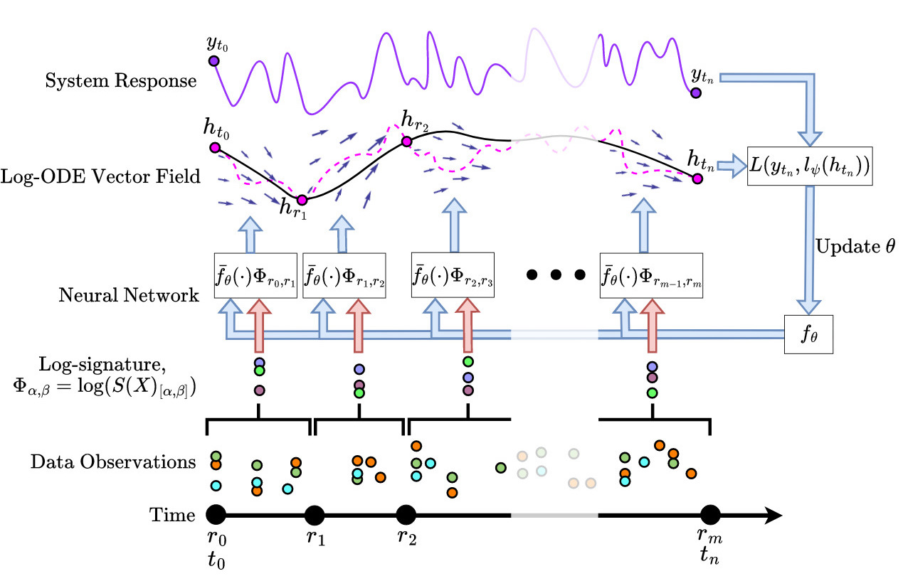
but with two major changes. First, instead of parameterising using a neural network, it is constructed using the iterated Lie brackets of a NCDE’s neural network, , via (17) and (18). Second, is ensured to be a function for . Figure 1 is a schematic diagram of the Log-NCDE method.
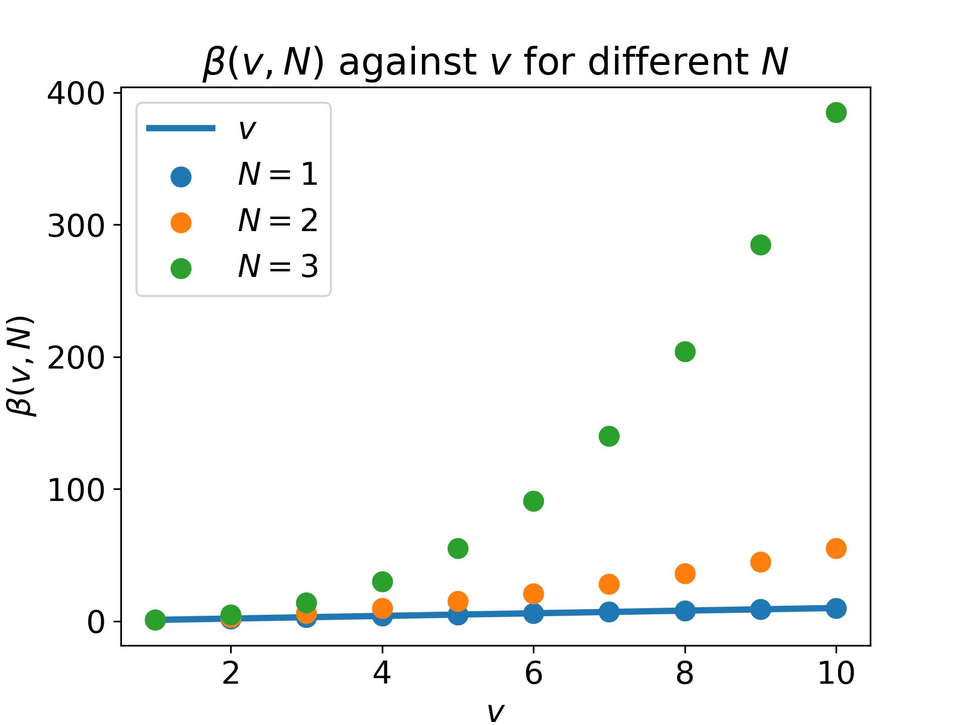
These changes have two benefits. The first is that the output dimension of is , whereas the output dimension of is . Figure 2 compares these values for paths of dimension from to and truncation depths of . For , Log-NCDEs are exploring a significantly smaller output space during training than NRDEs, while maintaining the same expressivity, as NCDEs are universal approximators. The second benefit of these changes is that and are no longer hyperparameters which impact the model’s architecture. Instead, they control the error in the approximation arising from using the Log-ODE method. This allows them to be changed during training and inference. Both of these benefits come at the cost of needing to calculate the iterated Lie brackets when evaluating Log-NCDEs, which will be quantified in section 3.4.
When , (19) simplifies to
| (20) |
Hence, in this case the only difference between Log-NCDEs and NRDEs is the regularisation of . Furthermore, (20) and (3) are equivalent when is a linear interpolation, so the approach of NCDEs, NRDEs, and Log-NCDEs all coincide when using a depth Log-ODE approximation [8].
3.2 Neural Networks
The composition of two functions is [20, Lemma 2.2]. Hence, a simple approach to ensuring a fully connected neural network (FCNN) is is to make each layer . This can be achieved by choosing an infinitely differentiable activation function, such as SiLU [21]. However, in practice this may not be enough regularity, as demonstrated by the following theorem.
Theorem 3.1.
Let be a FCNN with input dimension , hidden dimension , depth , and activation function SiLU. Assuming the input satisfies for , then and
| (21) |
where is a constant depending on and , and are the weights and biases of layer of , and is a polynomial of order .
Proof.
A proof is given in appendix B. ∎
Assuming that each layer of satisfies , an explicit evaluation of (21) gives
| (22) |
For a depth FCNN, this is greater than the maximum value of a double precision floating point number. Hence, it may be necessary to control explicitly during training. This is achieved by modifying the neural network’s loss function to
| (23) |
where is a hyperparameter controlling the weight of the penalty. This is an example of weight regularisation, which has long been understood to improve generalisation in NNs [22, 23]. Equation 23 is specifically a variation of spectral norm regularisation [24].
In the experiments conducted for this paper, Log-NCDEs use a FCNN with SiLU activation functions as their vector field . Empirically, the regularisation proposed to control the norm is only beneficial on some datasets. Therefore, is chosen using a hyperparameter optimisation with as an option.
3.3 Constructing the Log-ODE Vector Field
The linear map in (19) is defined recursively by (17) and (18). Assuming is infinitely differentiable, then is an element of the Lie algebra and
| (24) |
Let be the usual basis of . A choice of basis for is a Hall basis, denoted , which is a specific subset of up to the iterated Lie brackets of [25]. Rewriting (19) using a Hall basis,
| (25) |
where is the term in the log-signature corresponding to the basis elements . Since each can be written as iterated Lie brackets of , it is now possible to replace with the iterated Lie brackets of using (17) and (18). The are the vector fields defined by the columns of the neural network’s output. Hence, the vector field is evaluated at a point using Jacobian-vector products of the neural network, which can be efficiently calculated using forward-mode automatic differentiation.
3.4 Computational Cost
Constructing the iterated Lie brackets of incurs an additional computational cost for each evaluation of the vector field. In order to quantify this additional cost, assume that a NCDE, NRDE, and Log-NCDE are all using an identical FCNN as their vector field, except for the dimension of the final layer in the NRDE. Let denote the dimension of the hidden layers, and be the cost of evaluating the vector field of the NCDE. Then for a dimensional input path, the cost of evaluating a NRDE’s vector field is and the cost of evaluating a Log-NCDE’s vector field is [26]. The idea behind NRDEs and Log-NCDEs is that their additional cost is compensated for by the Log-ODE method requiring less vector field evaluations to attain a solution to the CDE of similar accuracy as other methods [27]. The idea behind Log-NCDEs, is that the additional cost of constructing the Lie brackets is compensated for by the smaller output dimension of the model’s neural network when compared to NRDEs.
3.5 Limitations
In this paper, we only consider Log-NCDEs which use a depth or depth Log-ODE approximation. This is due to the following two limitations. First, there are no theoretical results explicitly bounding the norm of a neural network for . Second, as discussed in the previous section, the computational cost required to evaluate grows rapidly with the depth . This can make computationally infeasible, especially for high-dimensional time series. Another general limitation of NCDEs is the need to solve the differential equation recursively, preventing parallelisation. This is in contrast to structured state-space models, whose underlying model is a differential equation that can be solved parallel in time [28].
Despite these limitations, in the experiments conducted for this paper, Log-NCDEs significantly improve upon the test set accuracies of NCDEs and NRDEs. Furthermore, they achieve test set accuracies higher than current state-of-the-art deep learning approaches, including structured state-space models. We hope these results motivate the importance of further work on developing a complete implementation of the Log-ODE method for NCDEs.
4 Experiments
4.1 Baseline Methods
Log-NCDEs are compared against four models, which represent the state-of-the-art for a range of deep learning approaches to time series modelling. The first two are discrete methods; a recurrent neural network using LRU blocks and a structured state-space model, S5 [2, 1]. The other two baseline models are continuous; a NCDE using a Hermite cubic spline with backward differences and a NRDE [3, 8].
4.2 Toy Dataset
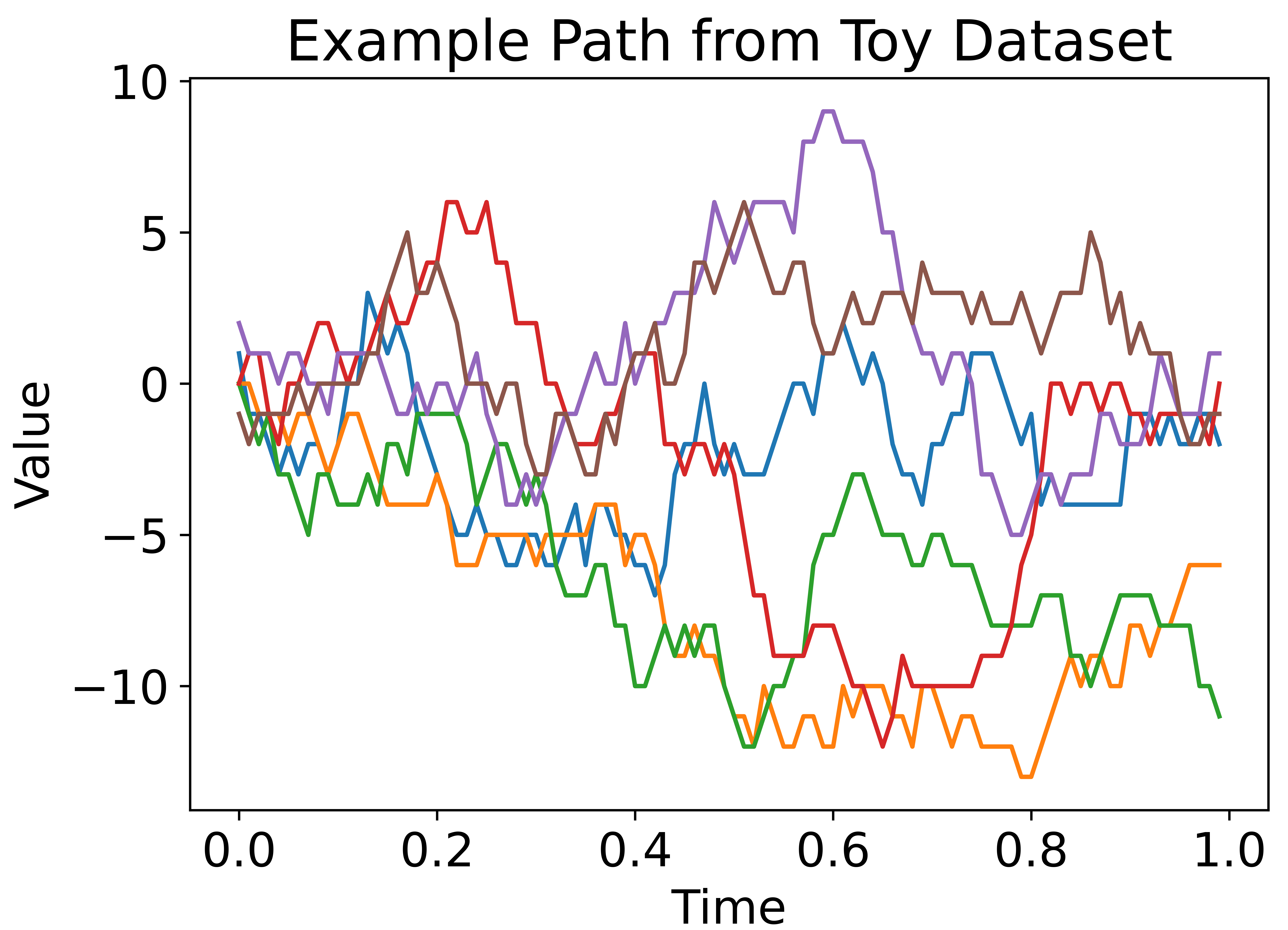
We construct a toy dataset with dimension and regularly spaced samples. For every time step, the change in each channel is sampled independently from the discrete probability distribution with density
| (26) |
where . In other words, the change in a channel at each time step is a sample from a standard normal distribution rounded to the nearest integer. Figure 3 is a plot of a sample path from the toy dataset.
We consider four different binary classifications on the toy dataset. Each classification is a specific term in the signature of the path which depends on a different number of channels.
-
1.
Was the change in the third channel, , greater than zero?
-
2.
Was the area integral of the third and sixth channels, , greater than zero?
-
3.
Was the volume integral of the third, sixth, and first channels, , greater than zero?
-
4.
Was the D volume integral of the third, sixth, first, and fourth channels, , greater than zero?
On this dataset, all models used a hidden state of dimension and Adam with a learning rate of . Both LRU and S5 used six blocks with GLU layers. S5 used a latent dimension of . NRDE and Log-NCDE used a stepsize of and a depth of .
4.3 UEA Multivariate Time Series Classification Archive
The models considered in this paper are evaluated on a subset of six datasets from the UEA multivariate time series classification archive (UEA-MTSCA). These six datasets were chosen via the following two criteria. First, only datasets with more than total cases were considered. Second, the six datasets with the most observations were chosen, as datasets with many observations have previously proved challenging for deep learning approaches to time series modelling. Following [8], the original train and test cases are combined and resplit into new random train, validation, and test cases using a split.
Hyperparameters for all models were found using a gird search over the validation accuracy on a fixed random split of the data. Full details on the hyperparameter grid search are in appendix C. Having fixed their hyperparameters, models are compared on their average test set accuracy over five different random splits of the data.
5 Results
5.1 Toy Dataset
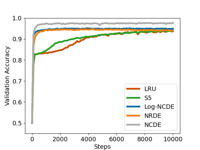
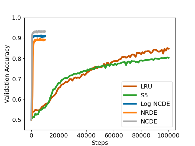
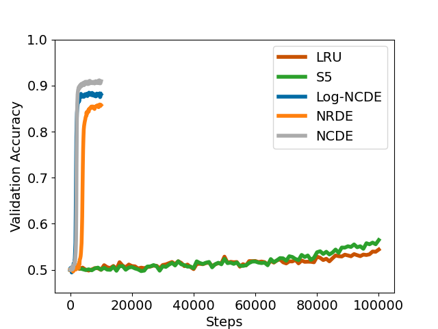
Figure 4 compares the performance of LRU, S5, NCDE, NRDE, and Log-NCDE on the four different classifications considered for the toy dataset. As expected, all of the models perform well when the label depends on one channel. As the number of channels the classification depends on increases, LRU and S5 begin to take significantly more training steps to converge. When the classification label is the volume integral containing four channels, S5 and LRU struggle to learn anything within steps of training. Increasing the number of training steps to , S5 and LRU are able to achieve validation accuracies of and respectively. However, this is still significantly lower than the validation accuracy achieved by NCDEs in steps of training.
As can be seen in figure 4, NCDEs outperform both NRDEs and Log-NCDEs using a stepsize of and a depth of . This is expected, as the classification labels considered are exactly the solution of a CDE, and for , NRDEs and Log-NCDEs are approximations to CDEs. Additionally, Log-NCDEs outperform NRDEs on each classification, with the gap in performance growing as the classification label depends on more channels.

| Dataset | Method | ||||
| S5 | LRU | NCDE | NRDE | Log-NCDE | |
| EigenWorms | |||||
| EthanolConcentration | |||||
| Heartbeat | |||||
| MotorImagery | |||||
| SelfRegulationSCP1 | |||||
| SelfRegulationSCP2 | |||||
| Average | |||||
| Average Rank | |||||
5.2 UEA-MTSCA
Table 1 reports the average and standard deviation of each model’s test set accuracy over five different splits of the data. On the datasets considered, NCDEs achieve the lowest average accuracy. NRDEs improve upon NCDEs in both average accuracy and rank, but are still outperformed by the current state-of-the-art models, LRU and S5. Log-NCDEs achieve the highest average accuracy and best average rank of the models considered. Furthermore, Log-NCDEs have the lowest standard deviation on four of the six datasets. These results highlight how the modifications introduced by Log-NCDEs can significantly increase performance.
6 Discussion
On the toy dataset, NCDEs, NRDEs, and Log-NCDEs are all able to model the dimensional volume integrals with high validation accuracy. This is not surprising, as the classification label can be written as a CDE driven by the input path. However, LRU and S5 both struggle to capture the necessary information as increases. Log-NCDEs outperforming NRDEs when the classification is the solution of a CDE indicate that NRDEs do not always converge to solutions where is the sum of Lie brackets of a NCDE vector field, .
On the UEA-MTSCA, the modifications Log-NCDEs make to NRDEs raise the average test set accuracy on all six datasets, and reduce the standard deviation on five datasets. These differences are signficant enough that Log-NCDEs achieve the highest average test set accuracy and best average rank. These results, alongside those on the toy dataset, demonstrate that calculating the Lie brackets and ensuring the neural network vector field is play an important role in applying the Log-ODE method to NCDEs.
7 Conclusion
Building on NRDEs, this paper introduced Log-NCDEs, which utilise the Log-ODE method to train NCDEs in an effective manner. This required proving a novel theoretical result bounding the norm of fully connected neural networks for , as well as developing an efficient method for calculating the iterated Lie brackets of a neural network. The experimental results presented in this paper demonstrate that explicitly constructing the Lie brackets when applying the Log-ODE method improves the performance of NCDEs to state-of-the-art.
There are many possible directions of future work. Log-NCDE’s could be extended to depth- Log-ODE methods for . This would require extending Theorem 3.1 to . Furthermore, it would be necessary to address the computational cost of the iterated Lie brackets, which could be done by using a structured neural network with cheap Jacobian-vector products as the CDE vector field. Another avenue could be to incorporate the recently developed adaptive version of the Log-ODE method [19].
8 Acknowledgements
Benjamin Walker and Terry Lyons were funded by the Hong Kong Innovation and Technology Commission (InnoHK Project CIMDA). Andrew McLeod and Terry Lyons were funded by the EPSRC [grant number EP/S026347/1] and The Alan Turing Institute under the EPSRC grant EP/N510129/1. Terry Lyons was funded by the Data Centric Engineering Programme (under the Lloyd’s Register Foundation grant G0095), the Defence and Security Programme (funded by the UK Government) and the Office for National Statistics & The Alan Turing Institute (strategic partnership).
References
- [1] Jimmy T.. Smith, Andrew Warrington and Scott W. Linderman “Simplified State Space Layers for Sequence Modeling” In International Conference on Learning Representations, 2023
- [2] Antonio Orvieto et al. “Resurrecting Recurrent Neural Networks for Long Sequences”, 2023 arXiv:2303.06349 [cs.LG]
- [3] Patrick Kidger, James Morrill, James Foster and Terry Lyons “Neural Controlled Differential Equations for Irregular Time Series” In Advances in Neural Information Processing Systems, 2020
- [4] Terry Lyons “Differential Equations Driven by Rough Signals (I): An Extension of an Inequality of L. C. Young” In Mathematical Research Letters 1, 1994, pp. 451–464
- [5] Patrick Kidger “On Neural Differential Equations”, 2022 arXiv:2202.02435 [cs.LG]
- [6] Tian Qi Chen, Yulia Rubanova, Jesse Bettencourt and David Duvenaud “Neural Ordinary Differential Equations.” In NeurIPS, 2018, pp. 6572–6583 URL: http://dblp.uni-trier.de/db/conf/nips/nips2018.html#ChenRBD18
- [7] Youness Boutaib, Lajos Gyurkó, Terry Lyons and Danyu Yang “Dimension-free Euler estimates of rough differential equations” In Revue Roumaine des Mathematiques Pures et Appliquees 59, 2013, pp. 25–53
- [8] James Morrill et al. “Neural Rough Differential Equations for Long Time Series” In International Conference on Machine Learning, 2021
- [9] S. Roman “Advanced Linear Algebra”, Graduate Texts in Mathematics Springer New York, 2007 URL: https://books.google.co.uk/books?id=bSyQr-wUys8C
- [10] C. Reutenauer “Free Lie Algebras”, LMS monographs Clarendon Press, 1993 URL: https://books.google.co.uk/books?id=cBvvAAAAMAAJ
- [11] T.J. Lyons, M. Caruana and T. Lévy “Differential Equations Driven by Rough Paths: École D’été de Probabilités de Saint-Flour XXXIV-2004”, Differential Equations Driven by Rough Paths: École D’été de Probabilités de Saint-Flour XXXIV-2004 no. 1908 Springer, 2007 URL: https://books.google.co.uk/books?id=WfgZAQAAIAAJ
- [12] Terry Lyons “Rough paths, Signatures and the modelling of functions on streams” arXiv, 2014 DOI: 10.48550/ARXIV.1405.4537
- [13] Imanol Perez Arribas “Derivatives pricing using signature payoffs” arXiv, 2018 DOI: 10.48550/ARXIV.1809.09466
- [14] Rimhak Ree “Lie Elements and an Algebra Associated With Shuffles” In Annals of Mathematics 68, 1958, pp. 210
- [15] Ilya Chevyrev and Andrey Kormilitzin “A Primer on the Signature Method in Machine Learning” arXiv, 2016 DOI: 10.48550/ARXIV.1603.03788
- [16] Andrea Bonfiglioli and Roberta Fulci “A New Proof of the Existence of Free Lie Algebras and an Application” In ISRN Algebra 2011, 2011 DOI: 10.5402/2011/247403
- [17] Kuo-Tsai Chen “Integration of Paths, Geometric Invariants and a Generalized Baker- Hausdorff Formula” In Annals of Mathematics 65, 1957, pp. 163
- [18] Alexander Kirillov “An Introduction to Lie Groups and Lie Algebras”, Cambridge Studies in Advanced Mathematics Cambridge University Press, 2008 DOI: 10.1017/CBO9780511755156
- [19] Christian Bayer, Simon Breneis and Terry Lyons “An Adaptive Algorithm for Rough Differential Equations”, 2023 arXiv:2307.12590 [math.NA]
- [20] Thomas Cass, Christian Litterer and Terry Lyons “New Trends in Stochastic Analysis and Related Topics: A Volume in Honour of Professor K. D. Elworthy”, Interdisciplinary mathematical sciences World Scientific, 2012 URL: https://books.google.co.uk/books?id=DCBqDQAAQBAJ
- [21] Stefan Elfwing, Eiji Uchibe and Kenji Doya “Sigmoid-weighted linear units for neural network function approximation in reinforcement learning” Special issue on deep reinforcement learning In Neural Networks 107, 2018, pp. 3–11 DOI: https://doi.org/10.1016/j.neunet.2017.12.012
- [22] Geoffrey E. Hinton “Learning Translation Invariant Recognition in Massively Parallel Networks” In Proceedings of the Parallel Architectures and Languages Europe, Volume I: Parallel Architectures PARLE Berlin, Heidelberg: Springer-Verlag, 1987, pp. 1–13
- [23] Anders Krogh and John A. Hertz “A Simple Weight Decay Can Improve Generalization” In Proceedings of the 4th International Conference on Neural Information Processing Systems, NIPS’91 Denver, Colorado: Morgan Kaufmann Publishers Inc., 1991, pp. 950–957
- [24] Yuichi Yoshida and Takeru Miyato “Spectral Norm Regularization for Improving the Generalizability of Deep Learning” In ArXiv abs/1705.10941, 2017
- [25] Marshall Hall “A basis for free Lie rings and higher commutators in free groups” In Proceedings of the American Mathematical Society, 1950
- [26] Andreas Griewank and Andrea Walther “Fundamentals of Forward and Reverse” In Evaluating Derivatives, 2000, pp. 31–59 URL: https://epubs.siam.org/doi/abs/10.1137/1.9780898717761.ch3
- [27] J.. Gaines and T.. Lyons “Variable Step Size Control in the Numerical Solution of Stochastic Differential Equations” In SIAM Journal on Applied Mathematics 57.5, 1997, pp. 1455–1484 DOI: 10.1137/S0036139995286515
- [28] Albert Gu, Karan Goel and Christopher Ré “Efficiently Modeling Long Sequences with Structured State Spaces” In International Conference on Learning Representations, 2022
- [29] Elias M. Stein “Singular Integrals and Differentiability Properties of Functions (PMS-30)” Princeton University Press, 1970 URL: http://www.jstor.org/stable/j.ctt1bpmb07
- [30] L.. Young “An inequality of the Hölder type, connected with Stieltjes integration” In Acta Mathematica 67, 1936, pp. 251–282
- [31] Terry J. Lyons “Differential equations driven by rough signals.” In Revista Matemática Iberoamericana 14.2, 1998, pp. 215–310 URL: http://eudml.org/doc/39555
- [32] Horatio Boedihardjo, Xi Geng, Terry Lyons and Danyu Yang “The signature of a rough path: Uniqueness” In Advances in Mathematics 293, 2016, pp. 720–737 DOI: https://doi.org/10.1016/j.aim.2016.02.011
- [33] Terry Lyons and Zhongmin Qian “Path Integration Along Rough Paths” In System Control and Rough Paths Oxford University Press, 2002 DOI: 10.1093/acprof:oso/9780198506485.003.0005
Appendix A Additional Mathematical Details
A.1 Functions
Definition A.1.
Let and be Banach spaces and denote the space of linear mappings from to .
In this paper, we will always take spaces of linear maps to be equipped with their operator norms.
Definition A.2.
A linear map is symmetric if for all and all bijectiive functions ,
| (27) |
The set of all symmetric linear maps is denoted
Definition A.3.
[29] Let be a non-negative integer, be a real number, a closed subset of , and . For , let . The collection is an element of if there exists such that for ,
| (28) |
and for , all , and each ,
| (29) |
When there is no confusion over and , the shorthand notation will be used. If a collection is , then the norm, denoted , is the smallest for which (28) and (29) hold.
In order to illustrate the definition of , two examples are given. When , then and implies is bounded and Hölder continuous. When , then is bounded and Lipschitz. When , then and if is bounded and there exists that is bounded, Hölder continuous, and satisfies
| (30) |
for all and some constant .
A.2 Existence and Uniqueness
Let and be continuous paths. The existence and uniqueness of the solution to a CDE,
| (31) |
depends on the smoothness of the control path and the vector field . We will measure the smoothness of a path by the smallest for which the variation is finite and the smoothness of a vector field by the largest such that the function is (defined in section A.1).
Definition A.4.
(Partition) A partition of a real interval is a set of real numbers satisfying .
Definition A.5.
(variation [30]) Let be a Banach space, be a partition of , and be a real number. The variation of a path is defined as
| (32) |
Theorem A.6.
Theorem A.7.
These theorems extend the classic differential equation existence and uniqueness results to controls with unbounded variation but finite variation for . A proof of these theorems is can be found in [11]. These theorems are sufficient for the differential equations considered in this paper. However, there are many settings where the control has infinite variation for all , such as Brownian motion. The theory of rough paths was developed in order to give meaning to (31) when the control’s variation is finite only for [31]. An introduction to rough path theory can be found in [11].
A.3 Norm of Tensor Product Space
Let be a Banach space and denote the tensor powers of ,
| (33) |
There is choice in the norm of . In this paper, we follow the setting of [32] and [33]. It is assumed that each is endowed with a norm such that the following conditions hold for all and :
-
1.
for all all bijectiive functions ,
-
2.
,
-
3.
for any bounded linear functional on and on , there exists a unique bounded linear functional on such that
Definition A.8.
(The Tensor Algebra [11]) For , let be equipped with a norm satisfying the above conditions, and define . The tensor algebra space is the set
| (34) |
with product defined by
| (35) |
The tensor algebra’s product is associative and has unit . As is an associative algebra, it has a Lie algebra structure, with Lie bracket
| (36) |
for [10].
Appendix B Proof of Theorem 3.1
The proof of theorem 3.1 relies on two lemmas. The first is a bound on the norm of the composition of two functions. The second is a bound on the norm of each layer of a fully connected neural network (FCNN).
B.1 Composition of Functions
Lemma B.1.
(Composed norm [20]) Let , , and be Banach spaces and and be closed. For , let and . Then the composition is with
| (37) |
where is the unique integer such that and is a constant independent of and .
The original statement of lemma B.1 in [20] gives (37) as
| (38) |
We believe this is a small erratum, as for defined as , (38) implies there exists such that
| (39) |
for all bounded and Lipschitz . As a counterexample, for any , take with . The following proof of lemma B.1 is given in [20].
Proof.
Bounding the norm of a neural network (NN) requires an explicit form for in (37). This can be obtained via the explicit calculations mentioned in the proof of lemma B.1. Here, we present the case .
Lemma B.2.
Let , , and be Banach spaces and and be closed. For , let and . Consider and defined for and by
| (40) |
Then and
| (41) |
Proof.
From definition A.3, , , and . Furthermore, for all
| (42) |
Similarly, for all we have that
| (43) |
Define and by
| (44) | ||||
for any and . Then
| (45) | ||||
Similarly, define and by
| (46) | ||||
for and . Then,
| (47) | ||||
Define and as in (40),
| (48) |
for and . Finally, define remainder terms and by
| (49) | ||||
for and . We now establish that and that the norm estimate claimed in (41) is satisfied.
First we consider the bounds on and . For any , (I) in (43) implies that
| (50) |
since . Further, for any and any , (43) and (II) in (42) imply that
since . Taking the supremum over with unit -norm, it follows that
| (51) |
Now we consider the bounds on and . For this purpose we fix and . We first assume that . In this case we may use (50) and (51) to compute that
Since means that , we deduce that
| (52) |
Similarly, we may use (51) and that to compute that
| (53) |
Taking the supremum over with unit -norm in (53) yields the estimate that
| (54) |
Together, (52) and (54) establish the remainder term estimates required to conclude that
in the case that .
We next establish similar remainder term estimates when . Thus we fix and assume that .
Note that means that . Additionally,
| (55) | ||||
where (II) in (42) and (I) in (45) have been used. We now consider the term . We start by observing that
Consequently, by using (II) in (43) to estimate the term , (I) in (45) to estimate the term , and (I) in (47) to estimate the term , we may deduce that
| (56) |
The combination of (55) and (56) yields the estimate
| (57) |
Turning our attention to , we fix and compute that
Consequently, by using (II) in (43) to estimate the term , (II) in (42) to estimate the term , (II) in (45) to estimate the term , and (II) in (47) to estimate the term , we may deduce that
| (58) |
The combination of (55) and (58) yields the estimate that
| (59) |
Taking the supremum over with unit -norm in (59) yields the estimate that
| (60) |
Finally, we complete the proof by combining the various estimates we have established for to obtain the -norm bound claimed in (41).
We start this task by combining (52) and (57) to deduce that for every we have
| (61) |
Moreover, the combination of (54) and (60) yields the estimate that
| (62) |
A consequence of (61) is that
| (63) |
whilst a consequence of (62) is that
| (64) |
Therefore, by combining (50), (51), (63), and (64), we conclude both that and that
| (65) |
∎
B.2 norm of a Neural Network Layer
Lemma B.2 allows us to bound the norm of a neural network (NN) given a bound on the norm of each layer of a NN. We demonstrate this here for a simple NN.
Definition B.3.
(Fully Connected NN) Let and be a fully connected NN with layers, input dimension , output dimension , hidden dimension , and activation function . Given an input , the output of the NN is defined as
| (67) |
where , for , and . Each layer is defined by
| (68) |
where , and are the learnable parameters and
| (69) |
Definition B.4.
(SiLU [21]) The activation function is defined as
| (70) |
Lemma B.5.
Let be a fully connected NN with activation function SiLU. Assume the input is normalised such that satisfies for . Then
| (71) |
where
| (72) |
Proof.
First, consider , where is the set of satisfying for . Each is composed of a linear layer and a SiLU. First, we show that
| (73) |
where So,
| (74) |
and
| (75) |
Since is at least twice differentiable,
| (76) |
where for some and . Similarly,
| (77) |
where for some . Now,
| (78) |
which has one non-zero eigenvalue
| (79) |
satisfying
| (80) |
Therefore,
| (81) |
and
| (82) |
The calculations for subsequent layers are very similar, except that the input to each layer is no longer restricted to . For example,
| (83) | ||||
In general
| (84) |
where
| (85) |
∎
B.3 Proof of Theorem 3.1
Theorem B.6.
Let be a FCNN with input dimension , hidden dimension , depth , and activation function SiLU [21]. Assuming the input satisfies for , then and
| (86) |
where is a constant depending on and , and are the weights and biases of layer of , and is a polynomial of order .
Appendix C UEA-MTSCA Hyperparameter Optimisation
NCDEs, NRDEs, and Log-NCDEs use a single linear layer as . NCDEs and NRDEs use FCNNs as their vector fields configured in the same way as their original papers [3, 8]. NCDEs use ReLU activation functions for the hidden layers and a final activation function of . NRDEs use the same, but move the activaion function to be before the final linear layer in the FCNN. NRDEs and Log-NCDEs take their intervals to be a fixed number of observations, referred to as the Log-ODE step. NCDEs, NRDEs, and Log-NCDEs all use Heun as their differential equation solver with a fixed stepsize of , with for NCDEs. Table 2 gives an overview of the different hyperparameters optimised over for each model on the UEA-MTSCA. The optimisation was performed using a grid search of the validation accuracy.
| Hyperparameters | Method | ||||
| S5 | LRU | NCDE | NRDE | Log-NCDE | |
| Learning Rate | |||||
| Time Included | True False | True False | True False | True False | True False |
| Hidden Dimension | 16 64 128 | 16 64 128 | 16 64 128 | 16 64 128 | 16 64 128 |
| Vector Field (Depth, Width) | - | - | (2, 32) (3, 64) (3, 128) (4, 128) | (2, 32) (3, 64) (3, 128) (4, 128) | (2, 32) (3, 64) (3, 128) (4, 128) |
| Log-ODE (Depth, Step) | - | - | - | (1, 1) (2, 2) (2, 4) (2, 8) (2, 12) (2, 16) | (1, 1) (2, 2) (2, 4) (2, 8) (2, 12) (2, 16) |
| Regularisation | - | - | - | - | 0.001 0.000001 0.0 |
| Number of Layers | 2 4 6 | 2 4 6 | - | - | - |
| State Dimension | 16 64 256 | 16 64 256 | - | - | - |
| S5 Blocks | 2 4 8 | - | - | - | - |