Abstract

In the rapidly evolving landscape of deep learning, the quest for models that balance expressivity with computational efficiency has never been more critical. This paper introduces Orchid, a novel architecture that reimagines sequence modeling by incorporating a new data-dependent convolution mechanism. Orchid is designed to address the inherent limitations of traditional attention mechanisms, particularly their quadratic complexity, without compromising the ability to capture long-range dependencies and in-context learning. At the core of Orchid lies the data-dependent convolution layer, which dynamically adjusts its kernel conditioned on input data using a dedicated conditioning neural network. We design two simple conditioning networks that maintain shift equivariance in the adaptive convolution operation. The dynamic nature of data-dependent convolution kernel, coupled with gating operations, grants Orchid high expressivity while maintaining efficiency and quasilinear scalability for long sequences. We rigorously evaluate Orchid across multiple domains, including language modeling and image classification, to showcase its performance and generality. Our experiments demonstrate that Orchid architecture not only outperforms traditional attention-based architectures such as BERT and Vision Transformers with smaller model sizes, but also extends the feasible sequence length beyond the limitations of the dense attention layers. This achievement represents a significant step towards more efficient and scalable deep learning models for sequence modeling.

1 Introduction

In the realm of modern deep neural networks, attention mechanisms have emerged as a gold standard, pivotal in domains such as natural language processing, image, and audio processing, and even complex fields like biology vaswani2018attention; dosovitskiy2020image; dwivedi2020generalization. However, despite their strong sequence analysis capabilities, these mechanisms suffer from their high computational complexity, which scales quadratically with sequence length, hindering their application to long-context tasks. This complexity has driven a shift towards innovative solutions to overcome this computational barrier, enabling analysis of long sequences in areas like genomics, DNA sequencing, and the creation of long musical compositions.

Researchers have explored various strategies to tackle the computational bottleneck of traditional dense attention layers tay2022efficient. One key strategy involves sparsifying the dense attention matrix. Instead of calculating the entire matrix, qiu2019blockwise; parmar2018image focus on specific local blocks of the receptive fields of sequences by chunking them into fixed-size blocks. Moreover, Sparse Transformer (child2019generating), Longformer (beltagy2020longformer) and BigBird zaheer2020big use strided attention patterns combined with local sliding windows to reduce computation. In contrast to using pre-determined patterns, other techniques include learning to cluster/sort tokens based on a similarity function, thereby enhancing the global view of the sequence, as seen in Reformer (kitaevreformer), Routing Transformer (roy2020efficient) Sparse Sinkhorn attention (tay2020sparse). Another approach involves low-rank approximations of the self-attention matrix, leveraging the insight that these matrices often exhibit low-rank properties, as demonstrated by Linformer wang2020linformer which projects keys and values matrices to lower-dimensional representation matrices. Another paradigm to reduce quadratic computation cost, is to replace the dot-product similarity between keys and query matrices of attention mechanism with a kernel function and avoid explicitly computing the attention matrix (katharopoulos2020transformers). Notable examples in this family include Performers (choromanski2020rethinking), Random Feature Attention (peng2021random) that are based on random feature approximation of the kernel function. Additionally, some models leverage a combinations of such techniques to design an efficient transformer (zhu2021long; zhang2021poolingformer). However, while these methods significantly reduce computational overhead, they may sacrifice expressiveness and performance, often requiring hybrid approaches that combine them with dense attention layers mehta2022long; fu2023hungry. On the other hand, recent works have aimed at sparsifying dense linear layers, used for feature mixing in Transformer blocks, to tackle another major source of high computation and memory demand in large models dao2022monarch; chen2021pixelated; chen2021scatterbrain.

Finding sub-quadratic and hardware-efficient mixing operators that are also expressive remains a significant challenge. Recent studies have explored attention-free solutions, particularly using state space models (SSMs) and long convolutions (gu2021efficiently; romero2021ckconv; mehta2022long; wang2022pretraining; fu2023hungry; poli2023hyena). A state space model characterizes a dynamical system’s behavior in terms of its internal state using a state equation, describing the dynamics of the system using first-order differential equations over the states, and an observation equation, relating state variables to observed outputs. A key insight is that SSMs can be formulated as a long convolution model between the input and output sequences (gu2021combining), allowing parallel and efficient training. However, recent work by poli2023hyena demonstrated that directly parameterizing the filter impulse response of the long-convolution leads to an even more expressive sequence mixing layer.

This paper proposes a novel data-dependent convolution mechanism to tackle the inherent quadratic complexity of traditional attention mechanisms, while maintaining the model’s ability to capture long-range dependencies and in-context learning. The data-dependent convolution layer dynamically adjusts its kernel based on input data using a dedicated conditioning neural network. We design two simple yet effective conditioning networks that maintain shift equivariance in the adaptive convolution operation. By combining these adaptive mechanisms with gating operations, our proposed model—named Orchid—achieves high expressivity while offering quasilinear scalability (with a complexity of $\mathcal{O}(L\log L)$) for long sequences. Evaluation across various domains, including language modeling and image classification, demonstrates the Orchid architecture’s performance and generality, outperforming attention-based architectures, like BERT and Vision Transformers, with smaller model sizes. Moreover, its allows for handling very large sequence lengths that are beyond the limitations of the dense attention layers. This achievement lays the foundation for further advancements in more efficient and scalable sequence modeling architectures.

2 Background

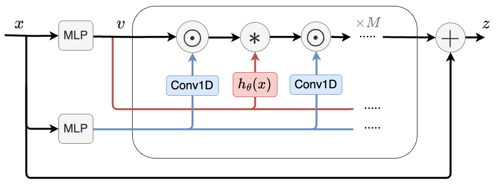
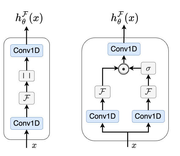
Figure 2.1: Orchid block. $\odot$ and $*$ denote element-wise multiplication and the convolution operator, respectively. The convolutions are implemented in the frequency domain using FFT. On the right two different conditioning networks, introduced in equations (2) and (3) as shift-invariant convolution kernels, are depicted.

Self-Attention Mechanism:

Given a length-$L$ sequence of embeddings (of tokens) ${\bm{x}}=(x_{1},x_{2},\ldots,x_{L})$, self-attention generates a new sequence by computing a weighted sum of these embeddings. It does this by linearly projecting ${\bm{x}}$ into three components: queries (${\bm{Q}}$), keys (${\bm{K}}$), and values (${\bm{V}}$), i.e.,

$${\bm{Q}}={\bm{x}}{\bm{W}}^{Q},\quad{\bm{K}}={\bm{x}}{\bm{W}}^{K},\quad{\bm{V}}={\bm{x}}{\bm{W}}^{V}.$$

Each head of a self-attention (SA) can be expressed as a dense linear layer as follows:

$${\bm{y}}={\sf SA}({\bm{Q}},{\bm{K}},{\bm{V}})={\sf SoftMax}\left(\frac{{\bm{Q}}{\bm{K}}^{T}}{\sqrt{d_{k}}}\right){\bm{V}}={\bm{A}}(x){\bm{V}},$$

where the matrix ${\bm{A}}(x)$ is populated with the attention scores between each pair of tokens. This description of the attention layer highlights its notable benefits, including its capability to capture long-range dependencies efficiently, with a sublinear parameter count. The attention mechanism enables direct computation of interactions between any two positions in the input sequence, regardless of their distance, without a corresponding rise in parameter counts. Additionally, the attention layer implements a data-dependent dense linear filter, effectively filtering the input while the filter weights are conditioned by a mapping of the data. This property makes it expressive and flexible enough to encode a large family of linear functions. However, these benefits come at the expense of quadratic computational complexity and memory costs.

This motivates us to develop an efficient and scalable data-dependent convolution mechanism, featuring a dynamic (adaptive) kernel that adjusts based on the input data. The kernel size of this convolution layer is as long as the input sequence length, allowing the capture of long-range dependencies across the input sequence while maintaining high scalability.

Linear Convolution:

Discrete-time linear convolution is a fundamental operation in digital signal processing that calculates the output as the weighted sum of the finite-length input ${\bm{x}}$ with shifted versions of the convolution kernel, ${\bm{h}}$, also known as the impulse response of a linear time-invariant (LTI) system. Formally it can be written as

$${\bm{y}}[t]=({\bm{h}}*{\bm{x}})[t]\triangleq\sum_{\ell=0}^{L-1}h[t-\ell]x[\ell].$$

In this definition, the output is a linear filter of the zero-padded input and convolution kernel. However, other padding schemes leads to different forms of convolution. A well-known form is circular convolution, defined as

$${\bm{y}}[t~{}{\sf mod}~{}L]=({\bm{h}}\circledast{\bm{x}})[t]\triangleq\sum_{\ell=0}^{L-1}h[t-\ell~{}{\sf mod}~{}L]x[\ell],$$

which is equivalent to the linear convolution of two sequences when one is cyclically padded at its boundaries.

Long Convolution and Fast Convolution Algorithm:

In standard convolution layers, the operation is explicitly parameterized with limited number of parameters. However, capturing long-range dependencies and correlations often requires a kernel as long as the input sequence, resulting in linear growth in parameter counts and also quadratic computational complexity. To address these challenges, firstly, we can retain sub-linear parameter scaling by implicitly parameterizing the convolution kernel with a multilayer perceptron (MLP) karami2019invertible; romero2021ckconv; poli2023hyena. On the other hand, one key advantage of convolution operators is that, according to the convolution theorem, they can be efficiently performed in the frequency domain using Fast Fourier Transform (FFT) algorithms (cooley1965FFT) resulting in $\mathcal{O}(L\log L)$ complexity. Formally, the linear convolution can be expressed as $\hat{{\bm{y}}}=\mathcal{F}^{-1}(\mathcal{F}(\hat{{\bm{h}}})\odot\mathcal{F}(\hat{{\bm{x}}}))={\bm{T}}^{-1}({\bm{h}}^{\mathcal{F}}\odot{\bm{T}}\hat{{\bm{x}}})$, where ${\bm{T}}$ is the DFT matrix, $\mathcal{F}$ denotes the discrete Fourier transformation, and $\hat{{\bm{x}}}$ denotes the zero-padded signal, defined as $\hat{{\bm{x}}}\triangleq{\sf pad_{2L}}({\bm{x}})=[\mathbf{0}_{L};~{}{\bm{x}}]$. Additionally, the circular convolution can be simply computed as: ${\bm{y}}={\bm{h}}\circledast{\bm{x}}=\mathcal{F}^{-1}(\mathcal{F}({{\bm{h}}})\odot\mathcal{F}({{\bm{x}}}))$.

3 Orchid

This section introduces the Data-Dependent Convolution Filter, a novel operator aimed at increasing the expressiveness of convolution operations. This operator serves as the foundational building block for the Orchid layer, which we will explore later in the section.

3.1 Data-Dependent Convolution Filter

We hypothesize that making the convolutional kernel data-dependent allows the filter to adapt to the specific characteristics of its input, potentially capturing more complex patterns within the signal. Formally, the output of the filter is defined as:

$${\bm{y}}=h_{\theta}({\bm{x}})*{\bm{x}}=\text{NN}_{\theta}({\bm{x}})*{\bm{x}}$$ (1)

The key innovation is to replace the static convolutional kernel with a dynamically generated one based on the input data. This is achieved through a conditioning network, denoted as $h_{\theta}({\bm{x}})=\text{NN}_{\theta}({\bm{x}})$, parameterized by $\theta$. Since the conditioning network outputs a vector of the same length as the input sequence, each token in the input can "attend" to the entire signal with personalized weights learned based on the specific input representation. Convolving the surrounding context based on a data-dependent weighting scheme can potentially offer richer feature extraction compared to conventional static convolutional filters.

Shift Equivariance of Convolution:

In general, a discrete convolution exhibits shift equivariance. This property implies that shifting the input by a specific amount results in the output shifting by the same amount (ignoring boundary effects). In circular convolution, this is formally expressed as: ${\sf shift}_{m}({\bm{y}})={\bm{h}}\circledast{\sf shift}_{m}({\bm{x}})$ (bronstein2021geometric), where this property is true regardless of the boundary effects. Here, ${\sf shift}_{m}({\bm{x}})[t]$ denotes the shift operation, defined as ${\sf shift}_{m}({\bm{x}})[t]\triangleq{\bm{x}}[t+m]$.

This property is particularly important because it ensures the operator’s response is robust to shift of features within the input, thereby enhancing the model’s generalization capabilities. This inductive bias is at the core of the widespread success of convolution operations thomas1802tensor. Therefore, it is desirable to design conditioning network in the data-dependent convolution (1) to preserve shift equivariance property. To maintain this property for convolution operations, it is sufficient to design filter kernel to be shift invariant. In the following, we present two shift-invariant conditioning networks.

I) Suppressing the Phase of Frequency Components:

A circular shift of a sequence ${\bm{u}}$ amounts to multiplying its frequency components by a linear phase factor: $\mathcal{F}\big{(}{\sf shift}_{m}({\bm{u}})\big{)}[\omega]={\bm{u}}^{\mathcal{F}}[\omega]\cdot e^{-\frac{i2\pi}{L}\omega m}$ oppenheim1999discrete. Consider a function $g({\bm{x}})$ that’s shift-equivariant (such as a depthwise Conv1d()): $g({\sf shift}_{m}({\bm{x}}))={\sf shift}_{m}(g({\bm{x}}))$. Its frequency components after a spatial shift of its input can be expressed as:

$$\mathcal{F}\big{(}g({\sf shift}_{m}({\bm{x}})\big{)}[\omega]=\mathcal{F}\left(g({\bm{x}})\right)[\omega]\cdot e^{-\frac{i2\pi}{L}\omega m}.$$

By taking the magnitude (absolute value or squared) of these complex-valued frequency components, we eliminate the phase shift and achieve shift invariance. Hence, defining $h^{\mathcal{F}}({\bm{x}})=\big{|}\mathcal{F}\big{(}g({\bm{x}})\big{)}\big{|}$ satisfies shift invariance: $h^{\mathcal{F}}({\sf shift}_{m}({\bm{x}}))=h^{\mathcal{F}}({\bm{x}})$.

In our setup, we utilizes a 1D depthwise linear convolution ($\texttt{Conv1d}()$) with a short kernel length (typically 3-5) applied separately to each feature dimension. This is followed by a short convolution in the frequency domain. Consequently, the conditioning neural network is formulated as

$$h^{\mathcal{F}}_{\theta}({\bm{x}})=\texttt{Conv1d}\big{(}\big{|}\mathcal{F}\left(\texttt{Conv1d}({\bm{x}})\right)\big{|}\big{)}$$ (2)

This architecture choice aims to minimize the number of parameters and computational burden introduced by the conditioning network within the overall model.

II) Using Cross-Correlation to Achieve Shift Invariance

An alternative method for achieving shift invariance involves computing the cross-correlation between two versions of a signal. Consider $k({\bm{x}})$ and $q({\bm{x}})$ as two shift-equivariant functions, satisfying: $k({\sf shift}_{m}({\bm{x}}))={\sf shift}_{m}(k({\bm{x}}))$ and $q({\sf shift}_{m}({\bm{x}}))={\sf shift}_{m}(q({\bm{x}}))$. Define $h({\bm{x}})$ as the cross-correlation of $k({\bm{x}})$ and $q({\bm{x}})$, given by:

$$h({\bm{x}})[t]=(k({\bm{x}})\star q({\bm{x}}))[t]\triangleq\sum_{\ell=0}^{L-1}k({\bm{x}})[\ell]\cdot q({\bm{x}})[t+\ell~{}\text{ mod }L].$$

This operation essentially slides $q({\bm{x}})$ over $k({\bm{x}})$ and measures their similarity at different offsets. Remarkably, this cross-correlation function, $h({\bm{x}})$, is also shift invariant:

$$h({\sf shift}_{m}({\bm{x}})) =k({\sf shift}_{m}({\bm{x}}))\star q({\sf shift}_{m}({\bm{x}}))$$

$$={\sf shift}_{m}(k({\bm{x}}))\star{\sf shift}_{m}(q({\bm{x}}))$$

$$=k({\bm{x}})\star q({\bm{x}})=h({\bm{x}})$$

Furthermore, the convolution theorem allows us to efficiently compute the cross-correlation in the frequency domain: $h^{\mathcal{F}}({\bm{x}})=\mathcal{F}\left(k({\bm{x}})\star q({\bm{x}})\right)=k^{\mathcal{F}^{*}}({\bm{x}})\odot q^{\mathcal{F}}({\bm{x}})$ where $k^{\mathcal{F}^{*}}$ denotes the complex conjugate of $k^{\mathcal{F}}$ and $\odot$ represents element-wise multiplication.

Remark 3.1.

By setting $k({\bm{x}})=q({\bm{x}})=g({\bm{x}})$, we derive $h^{\mathcal{F}}({\bm{x}})=|g^{\mathcal{F}}({{\bm{x}}})|^{2}$, This implies that the cross-correlation approach generalizes the magnitude-based approach, demonstrating its versatility.

Similar to the previous approach, we utilize distinct 1D depth-wise short convolutions for both $k({\bm{x}})$ and $q({\bm{x}})$, followed by another convolution post cross-correlation in the frequency domain. As a result, the conditioning neural network is defined as

$$h^{\mathcal{F}}_{\theta}({\bm{x}})=$$ (3)

$$~{}~{}~{}~{}~{}\texttt{Conv1d}\Bigl{(}\mathcal{F}^{*}\left(\texttt{Conv1d}({\bm{x}})\right)\odot\sigma\bigl{(}\mathcal{F}\left(\texttt{Conv1d}({\bm{x}})\right)\bigr{)}\Bigr{)}.$$

Inspired by gating mechanism, we applied $\sigma()=\texttt{Sigmoid}()$ to one of the sequences in the frequency domain. Both conditioning functions, described in equations 2 and 3, are also schematically visualized in Figure 2.1.