On the exact solution for the Schrödinger equation

Abstract

For almost 75 years, the general solution for the Schrödinger equation was assumed to be generated by a time-ordered exponential known as the Dyson series. We discuss under which conditions the unitarity of this solution is broken, and additional singular dynamics emerges. Then, we provide an alternative construction that is manifestly unitary, regardless of the choice of the Hamiltonian, and study various aspects of the implications. The new construction involves an additional self-adjoint operator that might evolve in a non-gradual way. Its corresponding dynamics for gauge theories exhibit the behavior of a collective object governed by a singular Liouville’s equation that performs transitions at a measure $0$ set. Our considerations show that Schrödinger’s and Liouville’s equations are, in fact, two sides of the same coin, and together they become the unified description of quantum systems.

1 Introduction

"Thus, the task is, not so much to see what no one has yet seen; but to think what nobody has yet thought, about that which everybody sees," E. Schrödinger.

The Schrödinger equation (named after Erwin Schrödinger, who postulated the equation in 1925) is the fundamental equation that governs the wave function of a quantum-mechanical system Schro . The discovery of this linear differential equation was a significant landmark in the development of quantum mechanics. In basic terms, if a wave-function of a system is given at some moment $t_{0}$ (denoted by $\left|\Psi(t_{0})\right\rangle$) one can determine the wave-function at all the subsequent moments by solving landau Peskin

$$\frac{d}{dt}\left|\Psi(t)\right\rangle\,=\,-i\hat{H}\left|\Psi(t)\right\rangle.$$ (1)

As long as the Hamiltonian of the system $\hat{H}$ is expressible as a bounded self-adjoint operator with no time dependence, the solution of (1) is given by the unitary evolution

$$\left|\Psi(t)\right\rangle\,=\,\hat{U}(t,\,t_{0})\left|\Psi(t_{0})\right\rangle,\qquad\qquad\hat{U}(t,\,t_{0})=\exp\left[-i\int_{t_{0}}^{t}dt^{\prime}\,\hat{H}\right].$$ (2)

In various cases, the Hamiltonian of a quantum system includes a time dependent part, and thus equation (1) is replaced by

$$\frac{d}{dt}\left|\Psi(t)\right\rangle\,=\,-i\hat{H}(t)\left|\Psi(t)\right\rangle,\qquad or\qquad\frac{d\hat{U}(t,\,t_{0})}{dt}\,=\,-i\hat{H}(t)\,\hat{U}(t,\,t_{0}).$$ (3)

The widely known general solution for (3) is expressible by using the $\hat{T}$ operator freema ,

$$\hat{U}(t,\,t_{0})\,=\,\hat{T}\exp\left[-i\int_{t_{0}}^{t}dt^{\prime}\,\hat{H}(t^{\prime})\right].$$ (4)

Our claim in this paper is the following: instead of solutions (2) and (4) which are unitary strictly for bounded self-adjoint Hamiltonians, one can obtain a universal unitary solution by introducing an additional operator such that

As shall later be shown, the only consistent differential equation is solely that of wave mechanics, governed by a self-adjoint component $\hat{\mathcal{H}}(t)$ of the general Hamiltonian $\hat{H}(t)$,

$$\frac{d}{dt}\left|\Psi(t)\right\rangle\,=\,-i\hat{\mathcal{H}}(t)\left|\Psi(t)\right\rangle,\qquad or\qquad\frac{d\hat{\mathcal{P}}(t,\,t_{0})}{dt}\,=\,-i\hat{\mathcal{H}}(t)\,\hat{\mathcal{P}}(t,\,t_{0}).$$ (7)

The new operator $\mathcal{\hat{N}}(t,\,t_{0})$ from (6) is known as the "jump operator" (in the context of QM) or alternatively, the "normalization operator" (in the context of QFT.) In its defining relation the operator $\hat{U}^{-1}(t,\,t_{0})$ denotes the inverse of $\hat{U}(t,\,t_{0})$, and $\hat{U}^{\dagger-1}(t,\,t_{0})$ is the inverse of its adjoint. The inclusion of the operator $\mathcal{\hat{N}}(t,\,t_{0})$ is, in fact, a promotion of the familiar normalization procedure of a quantum states to operatoric level, such that it becomes a local procedure rather than a global one. In other words, instead of having normalization only as an asymptotic procedure, it is now ensured even at the intermediate times. From definition (6) it is already evident that the introduction of $\mathcal{\hat{N}}$ is not necessary if $\hat{U}$ from (4) is truly an exact unitary operator. In that case the adjoint operator coincides with the inverse operator, $\hat{U}^{\dagger}(t,\,t_{0})\,=\,\hat{U}^{-1}(t,\,t_{0})$ and $\hat{U}^{\dagger-1}(t,\,t_{0})\,=\,\hat{U}(t,\,t_{0})$, which leads to $\mathcal{\hat{N}}(t,\,t_{0})=\mathbf{\hat{1}}$. However, as we shall explicitly show, this simplification is generally not valid in various interesting situations, among them is the case of gauge theories.

This paper is organized as follows: in section 2 we explain for what reason the standard solution cannot always provide a unitary description for quantum systems. In section 3, we provide a proof for the validity of the new solution, discuss its properties, and compute the new corresponding perturbative construction. In section 4, we provide several practical demonstrations in which the new solution might differ from the current mainstream solution, both in QM and QFT. In section 5, we summarize the implications of our result on various aspects. In appendix A, the differential equation for $\hat{\mathcal{N}}$ is computed. In appendix B, the perturbative expansion for $\hat{\mathcal{P}}$ is computed in terms of the Fock space. Appendix C serves to discuss on the mathematical properties of the Cauchy principal value. In appendix D, we analyze a conditionally convergent integrals and show that they contain a contribution that exists only in the generalized sense. In appendix E, we examine our justification to apply the Fubini theorem when dealing with gauge theories. Depending on the academic situation of the author, a subsequent publication involving the computation of measurable cross sections might appear, further comparing the current and newly proposed solutions.

2 Normalization as a consequence of unboundedness

"To know what you know and what you do not know, that is true knowledge," Confucius.

In this part we review the standard argument that is considered a proof for the unitarity of $\hat{U}$. Our intention is to have a closer look at the necessary mathematical conditions involved there, and then discuss under what circumstances this argument can be invalidated. Afterwards, a new construction is motivated, in which unitarity becomes a robust property and no longer can be broken. Then, we move on to discuss the drawbacks of the iterative solution method that has led to the construction of $\hat{U}$ in the first place. And lastly, we characterize from the mathematical perspective the different choices of Hamiltonians for which our considerations become relevant.

2.1 Why is $\hat{U}$ not always unitary?

Our starting point is a quick reminder for the procedure that has led to the result shown in eq. (4). The central idea is to solve the differential equation (3) by iterations landau : at first turning the original differential equation to an integral equation, and then substituting the result "inside itself" repeatedly ,

$$\begin{split}&\hat{U}(t,\,t_{0})\,=\,\hat{\mathbf{1}}\,-\,i\int_{t_{0}}^{t}dt^{\prime}\>\hat{H}(t^{\prime})\,\hat{U}(t^{\prime},\,t_{0})\\ &\,\;\quad\qquad\,=\,\hat{\mathbf{1}}\,-\,i\int_{t_{0}}^{t}dt^{\prime}\>\hat{H}(t^{\prime})\left[\hat{\mathbf{1}}\,-\,i\int_{t_{0}}^{t^{\prime}}dt^{\prime\prime}\>\hat{H}(t^{\prime\prime})\,\hat{U}(t^{\prime\prime},\,t_{0})\right].\end{split}$$ (8)

The applicability of the iterative method is discussed in section 2.3, but for now let us assume the validity of this method. The series that is obtained by this process, known as the Dyson series freema , is given by

$$\begin{split}&\hat{U}(t,\,t_{0})\,=\,\hat{\mathbf{1}}\,-\,i\int_{t_{0}}^{t}dt^{\prime}\>\hat{H}(t^{\prime})\,-\,\int_{t_{0}}^{t}dt^{\prime}\,\hat{H}(t^{\prime})\,\int_{t_{0}}^{t^{\prime}}dt^{\prime\prime}\hat{H}(t^{\prime\prime})\,+\,\ldots\end{split}$$ (9)

At this point the terms of the series above should be interpreted as merely a schematic operatoric symbols. The convergence properties of the terms and of the series as a whole are dictated by the choice of the Hamiltonian as well as the time interval of the evolution. Let us now present the familiar argument that currently exist in the literature landau and regarded as a proof for the unitarity of $\hat{U}(t,t_{0})$. By assuming that one can replace the integrations in the iterative form with the productive form,

$$\hat{U}(t,\,t_{0})\,=\,\hat{\mathbf{1}}\,-\,i\int_{t_{0}}^{t}dt^{\prime}\>\hat{H}(t^{\prime})\,-\,\int_{t_{0}}^{t}dt^{\prime}\int_{t_{0}}^{t^{\prime}}dt^{\prime\prime}\,\hat{H}(t^{\prime})\,\hat{H}(t^{\prime\prime})\,+\,\ldots$$ (10)

And by further assuming the self-adjointness of the terms involved in the expansion (10) throughout the entire evolution,

$$\hat{U}^{\dagger}(t,t_{0})\,=\,\hat{\mathbf{1}}\,+\,i\int_{t_{0}}^{t}dt^{\prime}\>\hat{H}(t^{\prime})\,-\,\int_{t_{0}}^{t}dt^{\prime}\int_{t_{0}}^{t^{\prime}}dt^{\prime\prime}\>\hat{H}(t^{\prime\prime})\,\hat{H}(t^{\prime})\,+\,\ldots$$ (11)

From which it follows, by taking the product of (10) and (11), that

$$\begin{split}&\hat{U}^{\dagger}(t,t_{0})\,\hat{U}(t,t_{0})\,=\,\mathbf{\hat{1}}\,+\,\left(\int_{t_{0}}^{t}dt^{\prime}\>\hat{H}(t^{\prime})\right)^{2}\,-\,\int_{t_{0}}^{t}dt^{\prime}\int_{t_{0}}^{t^{\prime}}dt^{\prime\prime}\>\hat{H}(t^{\prime})\,\hat{H}(t^{\prime\prime})\\ &\qquad\qquad\qquad\quad\;-\,\int_{t_{0}}^{t}dt^{\prime}\int_{t_{0}}^{t^{\prime}}dt^{\prime\prime}\>\hat{H}(t^{\prime\prime})\,\hat{H}(t^{\prime})\,+\,\ldots\end{split}$$ (12)

The next step, as shown in figure 1, is to apply an "operatoric version" of the Fubini theorem Rudin and perform an exchange of the ordering of the two time integrations in the last term of (LABEL:uudag),

$$\int_{t_{0}}^{t}dt^{\prime}\int_{t_{0}}^{t^{\prime}}dt^{\prime\prime}\>\hat{H}(t^{\prime\prime})\,\hat{H}(t^{\prime})\,=\,\int_{t_{0}}^{t}dt^{\prime}\int_{t^{\prime}}^{t}dt^{\prime\prime}\>\hat{H}(t^{\prime})\,\hat{H}(t^{\prime\prime}).$$ (13)

Then, after introducing the replacement (13) in the result of (LABEL:uudag), the last two terms can be combined together,

$$\int_{t_{0}}^{t}dt^{\prime}\int_{t_{0}}^{t^{\prime}}dt^{\prime\prime}\>\hat{H}(t^{\prime})\,\hat{H}(t^{\prime\prime})\,+\,\int_{t_{0}}^{t}dt^{\prime}\int_{t^{\prime}}^{t}dt^{\prime\prime}\>\hat{H}(t^{\prime})\,\hat{H}(t^{\prime\prime})\,=\,\left(\int_{t_{0}}^{t}dt^{\prime}\,\hat{H}(t^{\prime})\right)^{2},$$ (14)

what allegedly seems to lead to the inevitable conclusion that $\hat{U}^{\dagger}(t,\,t_{0})\,=\,\hat{U}^{-1}(t,\,t_{0})$.

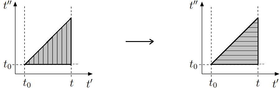
Figure 1: Changing the order of integration via the Fubini theorem. Left: the original integration. This integration was required to be performed on the triangle defined by first integrating the interval $t^{\prime\prime}\in[t_{0},\,t^{\prime}]$, and only then $t^{\prime}\in[t_{0},\,t]$. Right: the integration after applying the Fubini theorem – the first integration is carried on the interval $t^{\prime\prime}\in[t^{\prime},\,t]$.

Now, let us look again on the argument that has been presented above, but this time adopt a more cautious approach, paying attention to the mathematical conditions involved at each step that we perform. Before we proceed, a wise question to ask ourselves is – as which type of operator should we treat the general Hamiltonian? bounded or unbounded?

A detailed discussion about the differences between these two kinds of mathematical constructions can be found in Teschl unbounded . From there we learn that confidently answering the question above is necessary in order to determine the legitimate set of simplification operations that can be performed. For clarity, let us summarize the underlying requirements which took place while presenting the unitarity argument above:

Clearly, the externally imposed condition (15) significantly restricts the allowed set of possible choices of Hamiltonians for which unitarity is expected to be maintained. Our ability to perform operation (16) is mathematically justified only if the domains of the integrated operators on both sides is equivalent throughout the evolution. More importantly, in order to satisfy the property (17), the operator $\mathcal{\hat{O}}(t_{1})$ is required to be a bounded operator. A sufficient condition that ensures the validity of the unitarity argument is that the involved operators are Hilbert–Schmidt class Functionl , satisfying an analogous condition to absolute convergence for any choice of $\left|\psi\right\rangle\in\mathcal{D}(\hat{H})$,

$$\int_{t_{0}}^{t}dt^{\prime}\int_{t_{0}}^{t^{\prime}}dt^{\prime\prime}\>\left\|\hat{H}(t^{\prime\prime})\,\hat{H}(t^{\prime})\,\left|\psi\right\rangle\right\|_{\mathcal{Y}}^{2}\,<\,\infty\>.$$ (18)

However, in practical problems we often deal with situations in which the condition above is violated. That happens since either the integration interval is improper, or due to integrand containing singularities. In these cases the resulting integrals (potentially obtained after regularization procedure) converge only conditionally. As we show in appendix D, these integrals can be seen as involving contributions that exist only in the generalized sense, which demands a cautious treatment.

2.2 How to unitarize $\hat{U}$?

The main point of the last section was that unitarity is not a manifest property of $\hat{U}$, but rather a property that follows only under a certain restrictive assumptions. A significant advancement toward a manifestly unitary construction passes through the elimination of the time ordering operation, which is well defined only for finite times (unless, as we shall see, used in a specific combination.) Historically speaking, this problem was first addressed by W. Magnus in the seminal paper Magnus . Magnus asked himself the following question: how can we write an analogous expansion for $\hat{U}(t,\,t_{0})$ in a way which does not involve the time-ordering operator $\hat{T}$?

After all, the existence of such a representation is guaranteed as a fundamental property of unitary matrices as guaranteed by the Stone theoremstone . Magnus was able to show that under certain assumptions there exist an equivalent representation for (4) such that

$$\hat{T}\exp\left[-i\int_{t_{0}}^{t}dt^{\prime}\,\hat{H}(t^{\prime})\right]\,=\,\exp\left[-i\int_{t_{0}}^{t}dt^{\prime}\,\hat{\Omega}(t^{\prime})\right].$$ (19)

The self-adjoint operator $\hat{\Omega}(t)$ is the Magnus series generator (the dependence on the parameter $t_{0}$ is kept implicit) which can be written up to order $g^{3}$ as

$$\begin{split}&\hat{\Omega}(t)\,=\,\hat{H}(t)\,-\,\frac{i}{2!}\int_{t_{0}}^{t}dt^{\prime}\>\left[\hat{H}(t),\,\hat{H}(t^{\prime})\right]\\ &+\,\frac{i}{3!}\int_{t_{0}}^{t}dt^{\prime}\int_{t_{0}}^{t^{\prime}}dt^{\prime\prime}\>\left(\left[\hat{H}(t),\,\left[\hat{H}(t^{\prime}),\,\hat{H}(t^{\prime\prime})\right]\right]+\left[\hat{H}(t^{\prime\prime}),\,\left[\hat{H}(t^{\prime}),\,\hat{H}(t)\right]\right]\right).\end{split}$$ (20)

A more detailed analysis of the conditions under which these expansions are equivalent is discussed in Blnes . However, it is clear that establishing a complete equivalence for any type of Hamiltonian cannot be done in this way. Tackling the missing regime, in which the resulting integrations are conditionally convergent, requires a delicate approach in which one cannot perform any simplifying operation on the terms of the series. Essentially, the only way to proceed is by replacing (4) by an alternative construction. This can be done by unitarization of an operator carried by the replacement

$$\mathbf{\mathcal{\hat{O}}}\,\longrightarrow\,\sqrt{\mathbf{\mathcal{\hat{O}}}^{\dagger-1}\,\mathbf{\mathcal{\hat{O}}}^{-1}}\,\mathbf{\mathcal{\hat{O}}},$$ (21)

which leads to the proposed solution in (5). This decomposition is analogous to the polar decomposition, which always exists and is always unique polar . By construction, the solution $\mathcal{\hat{P}}(t,\,t_{0})$ manifestly preserves the exactness of unitarity at all orders and at all times,

$$\mathcal{\hat{P}}^{\dagger}(t,\,t_{0})\,\mathcal{\hat{P}}(t,\,t_{0})\,=\,\hat{U}^{\dagger}(t,\,t_{0})\,\hat{U}^{\dagger-1}(t,\,t_{0})\,\hat{U}^{-1}(t,\,t_{0})\,\hat{U}(t,\,t_{0})\,=\,\bm{\hat{1}},$$ (22)

from which it is immediately apparent that $\mathcal{\hat{P}}^{\dagger}(t,\,t_{0})\,=\,\mathcal{\hat{P}}^{-1}(t,\,t_{0})\,$. The expression for the inverse of $\hat{U}$ can be uniquely determined by the condition $\hat{U}^{-1}(t,\,t_{0})\,\hat{U}(t,\,t_{0})\,=\,\hat{\bm{1}}$ so that,

$$\hat{U}^{-1}(t,t_{0})\,=\,\hat{\mathbf{1}}+i\int_{t_{0}}^{t}dt^{\prime}\>\hat{H}(t^{\prime})-\left(\int_{t_{0}}^{t}dt^{\prime}\,\hat{H}(t^{\prime})\right)^{2}+\int_{t_{0}}^{t}dt^{\prime}\int_{t_{0}}^{t^{\prime}}dt^{\prime\prime}\>\hat{H}(t^{\prime})\,\hat{H}(t^{\prime\prime})\,+\,\ldots$$ (23)

By insertion back to (6) along with the Taylor expansion of the square root, the following result is obtained for the case of self-adjoint Hamiltonian:

$$\begin{split}&\mathcal{\hat{N}}(t,\,t_{0})\,=\,\mathbf{\hat{1}}\,-\,\frac{1}{2}\left(\int_{t_{0}}^{t}dt^{\prime}\,\hat{H}(t^{\prime})\right)^{2}\,+\,\frac{1}{2}\int_{t_{0}}^{t}dt^{\prime}\int_{t_{0}}^{t^{\prime}}dt^{\prime\prime}\,\left\{\hat{H}(t^{\prime}),\,\hat{H}(t^{\prime\prime})\right\}\,+\,\ldots\end{split}$$ (24)

Then, by using the definition (5), we find the expansion

$$\begin{split}&\mathcal{\hat{P}}(t,\,t_{0})\\ &=\,\mathbf{\hat{1}}\,-\,i\int_{t_{0}}^{t}dt^{\prime}\>\hat{H}(t^{\prime})\,-\,\frac{1}{2}\left(\int_{t_{0}}^{t}dt^{\prime}\>\hat{H}(t^{\prime})\right)^{2}\,-\,\frac{1}{2}\int_{t_{0}}^{t}dt^{\prime}\int_{t_{0}}^{t^{\prime}}dt^{\prime\prime}\>\left[\hat{H}(t^{\prime}),\,\hat{H}(t^{\prime\prime})\right]\,+\,\ldots\end{split}$$ (25)

However, generally the original terms must be kept in their full glory ,

$$\begin{split}&\hat{\mathcal{N}}(t,t_{0})\,=\,\hat{\mathbf{1}}+\frac{i}{2}\int_{t_{0}}^{t}dt^{\prime}\>\hat{H}(t^{\prime})-\frac{i}{2}\left(\int_{t_{0}}^{t}dt^{\prime}\>\hat{H}(t^{\prime})\right)^{\dagger}-\frac{3}{8}\left(\int_{t_{0}}^{t}dt^{\prime}\,\hat{H}(t^{\prime})\right)^{2}-\frac{3}{8}\left(\int_{t_{0}}^{t}dt^{\prime}\,\hat{H}(t^{\prime})\right)^{\dagger\,2}\\ &+\frac{1}{4}\left|\int_{t_{0}}^{t}dt^{\prime}\,\hat{H}(t^{\prime})\right|^{2}+\frac{1}{2}\int_{t_{0}}^{t}dt^{\prime}\hat{H}(t^{\prime})\int_{t_{0}}^{t^{\prime}}dt^{\prime\prime}\hat{H}(t^{\prime\prime})+\frac{1}{2}\left(\int_{t_{0}}^{t}dt^{\prime}\hat{H}(t^{\prime})\int_{t_{0}}^{t^{\prime}}dt^{\prime\prime}\hat{H}(t^{\prime\prime})\right)^{\dagger}\,+\,\ldots\end{split}$$ (26)

from which we arrive at the manifestly unitary result,

$$\begin{split}&\hat{\mathcal{P}}(t,t_{0})\,=\,\hat{\mathbf{1}}-\frac{i}{2}\int_{t_{0}}^{t}dt^{\prime}\>\hat{H}(t^{\prime})-\frac{i}{2}\left(\int_{t_{0}}^{t}dt^{\prime}\>\hat{H}(t^{\prime})\right)^{\dagger}+\frac{1}{8}\left(\int_{t_{0}}^{t}dt^{\prime}\>\hat{H}(t^{\prime})\right)^{2}-\frac{3}{8}\left(\int_{t_{0}}^{t}dt^{\prime}\>\hat{H}(t^{\prime})\right)^{\dagger\,2}\\ &-\frac{1}{4}\left|\int_{t_{0}}^{t}dt^{\prime}\,\hat{H}(t^{\prime})\right|^{2}-\frac{1}{2}\int_{t_{0}}^{t}dt^{\prime}\hat{H}(t^{\prime})\int_{t_{0}}^{t^{\prime}}dt^{\prime\prime}\hat{H}(t^{\prime\prime})+\frac{1}{2}\left(\int_{t_{0}}^{t}dt^{\prime}\hat{H}(t^{\prime})\int_{t_{0}}^{t^{\prime}}dt^{\prime\prime}\hat{H}(t^{\prime\prime})\right)^{\dagger}\,+\,\ldots\end{split}$$ (27)

As expected, we note that expressions (LABEL:tun) and (LABEL:pitarg2) indeed reduce to expressions (LABEL:exppnor) and (LABEL:pitarexp) under the assumption of a self-adjoint Hamiltonian. When handling the above expansions it is important to keep in mind that the property of linearity does not apply before expressing the integrand solely in terms of linear objects (branch independent.) Often, the presentation of such integrals will be defined by using an additional $\epsilon$ parameter and we would like to investigate the limit in which it is approaching to $0$ (see appendix B.) One should keep in mind that the additivity rule for limits is applicable only if the initial limits exist in the classical sense.

2.3 Why may the iterative method fail?

In this section we would like to discuss the Picard’s method of successive approximations Lindelof Evolutiona in order to analyze the capacity of this approach to yield the solution for a differential evolution equation of first order. Our intention is to consider the following differential equation:

$$\frac{dy}{dx}\,=\,f(x,y)\>,$$ (28)

subject to the initial condition $y(x_{0})=y_{0}$. The key point of Picard’s idea consist in replacing the original differential equation by a system of difference equations that approximate the evolution occurring in a small neighborhood of the domain lax . As demonstrated below, under certain assumptions, the resulting difference equation can reliably approximate the evolution on the whole domain. In that case, the resulting solution uniquely converges to the analytic solution of the original equation. Our intention is to provide an answer for the following fundamental question – what are the necessary conditions for the iterative method to be applicable? is the discretization limit always admissible?

Let us start by applying the method in the non-negative region $[0,\,x]$ with the simple choice of $f(x,y)\,=\,gy$ with $y_{0}=1$. The analytical solution corresponding to our choice can naturally be found by direct integration, $y(x)=e^{gx}$. Now let us reproduce the last solution via the iterative method. Our initial assumption is that the differential equation above allows to start a process of successive approximations by rewriting it in the integral form,

$$y_{n+1}(x)\,=\,y_{0}+\int_{0}^{x}dx^{\prime}\,f(x^{\prime},y_{n}(x^{\prime})).$$ (29)

After a few iterations the following results are obtained:

$$\begin{split}&y_{1}(x)\,=\,1+g\int_{0}^{x}1\,dx^{\prime}=1+gx,\\ &y_{2}(x)\,=\,1+g\int_{0}^{x}(1+gx)\,dx^{\prime}=1+gx+\frac{1}{2!}g^{2}x^{2},\\ &y_{3}(x)\,=\,1+g\int_{0}^{x}(1+gx+\frac{1}{2!}g^{2}x^{2})\,dx^{\prime}=1+x+\frac{1}{2!}g^{2}x^{2}+\frac{1}{3!}g^{3}x^{3},\end{split}$$ (30)

from which we observe the series that is generated after $n$ iterations,

$$y_{n}(x)\,=\,\sum_{i=0}^{n}\frac{g^{n}}{n!}x^{n}.$$ (31)

As expected, the sequence $\{y_{n}(x)\}$ converges to the Taylor series for the exponent,

$$\lim_{n\rightarrow\infty}y_{n}(x)\,=\,e^{gx}\,,$$ (32)

which indeed reproduced the expected result. This last equivalence was, in fact, guaranteed to us by the Picard–Lindelöf theorem Evolutiona . As lengthy discussed in byron , the error at the $n$th step of the iterative procedure in the interval $x_{0}-h<x<x_{0}+h$ with $h\,\equiv\,\min\left(a,\,\frac{b}{M}\right)$, where $\left|x-x_{0}\right|\,\leq\,a$ and $\left|y(x)-y_{0}\right|\,\leq\,b$, is bounded by the inequality

$$\left|y_{n}(x)-y(x)\right|\,\leq\,\frac{MN^{n-1}}{n!}h^{n},$$ (33)

with the definitions $M\,\equiv\,\max_{(x,y)\in\mathcal{D}}\left|f(x,y)\right|$, $N\,\equiv\,\max_{(x,y)\in\mathcal{D}}\left|\frac{\partial f}{\partial y}\right|$ . Clearly, in order for the solution obtained by iterative method to be considered valid, it must converge asymptotically to the analytic solution,

$$\lim_{n\rightarrow\infty}\left|y_{n}(x)-y(x)\right|\,=\,0.$$ (34)

However, as we are about to see, the above theorem will fail to imply uniqueness when singularities are involved. For example, let us take a closer look on what happens when trying to solve a differential equation with RHS involving Dirac delta function distrib ,

$$\frac{df(x)}{dx}\,=\,\delta(x-a)\,f(x),$$ (35)

subject to the initial condition $f(0)=1$ with $a>0$. The direct solution method leads to $f(x)\,=\,e^{\Theta(x-a)}$, where we have used the defining relation for the Heaveside theta function,

$$\int_{0}^{x}dx^{\prime}\,\delta(x^{\prime}-a)\,=\,\Theta(x-a).$$ (36)

Now let us try to reproduce the last result by the iterative method. For that purpose we present the solution as

$$f(x)\,=\,1+\int_{0}^{x}dx^{\prime}\,\delta(x^{\prime}-a)\,f(x^{\prime})\,,$$ (37)

and then by substitution

$$f(x)\,=\,1+\int_{0}^{x}dx^{\prime}\,\delta(x^{\prime}-a)\left[1+\int_{0}^{x^{\prime}}dx^{\prime\prime}\,\delta(x^{\prime\prime}-a)\,f(x^{\prime\prime})\right]\,.$$ (38)

After performing the integration of the inner brackets by using (36) it is clear that something goes wrong. One arrives at the badly defined result that involves integration over a product of two distributions Schwarz ,

$$\int_{0}^{x}dx^{\prime}\,\delta(x^{\prime}-a)\,\Theta(x^{\prime}-a)\;\longrightarrow\;\mathtt{Indeterminate}.$$ (39)

It is, therefore, clear that the iterative series (38) will not converge to the expected result. We realize that in order for the iterative method to work, the integrand has to be well defined (measurable function) at each part of the domain. A more practical example, which allows to get a deeper understanding what happens when the conditions for Picard theorem fails, is given by the differential equation,

$$x\frac{dy}{dx}\,=\,A,$$ (40)

which has an unbounded RHS when brought to the form of (28). The solution is often taken as $y(x)\,=\,A\log|x|+C$, although a more general discontinuous solution can be found,

$$y\,=\,\begin{cases}\begin{array}[]{c}A\log(x)+C\\ A\log(-x)+B\end{array}&\begin{array}[]{c}x>0\\ x<0.\end{array}\end{cases}$$ (41)

In terms of distributions that can be expressed as $y(x)\,=\,A\,\log|x|+(B-C)\,\Theta(-x)+C$. Note that even thought the constant term changes in the passage between the two disjoint regions, this is still valid a solution. The discontinuous part, or alternatively, the singular dynamics at $x=0$, is exactly the part in which the iterative procedure fails to provide a definitive answer. Thus, our main conclusion in this part is that singular differential equations cannot be solved by a solution method that is based solely on the iterative method.

2.4 How to classify quantum systems?

In this part we discuss the circumstances under which the solution $\hat{U}$ can no longer be considered a complete unitary description. This will be done by characterizing each of the three main types of Hamiltonians that typically play a role in problems of quantum physics.

2.4.1 The bounded self-adjoint evolution

One of the fundamental postulate in quantum mechanics is that any measurable dynamical quantity is represented by a self-adjoint operator satisfying the condition $(\ref{excher})$. Quantities such as the momentum of free particles or the energy of stable atoms and molecules are real numbers, therefore the operators which represent them must have real eigenvalues. A crucial property of the Hamiltonians belonging to this category is that they are also bounded opertors Functionl :

As a simple example for a practical realization of such an operator it is possible to use a matrix of finite dimensions $\hat{H}(t):L^{2}(\mathbb{R})\rightarrow L^{2}(\mathbb{R})$ with entries given by a finite valued and continuous functions:

$$\hat{H}(t)\,=\,f_{1}\,\hat{\sigma}_{1}+f_{2}\,\hat{\sigma}_{2}+f_{3}\,\hat{\sigma}_{3}\,=\,\left(\begin{array}[]{cc}f_{3}&f_{1}-if_{2}\\ f_{1}+if_{2}&-f_{3}\end{array}\right),$$ (43)

with $f_{i}=f_{i}(t)\in\mathbb{R}$ and $\left|f_{i}\right|\,<\,\infty$ where $i\in\left\{1,2,3\right\}$. In case that $t$ is finite, condition (42) implies for a self-adjoint Hamiltonians that

$$\left\|\left(\hat{U}(t_{2},\,t_{0})\,-\,\hat{U}(t_{1},\,t_{0})\right)\left|\psi(t_{0})\right\rangle\right\|_{\mathcal{H}_{2}}\,\leq\,\left\|2\left|\psi(t_{0})\right\rangle\right\|_{\mathcal{H}_{1}},$$ (44)

for any $t_{2},t_{1}\in[t_{0},t]$ and $\left|\psi(t_{0})\right\rangle\in\mathcal{H}_{1}$. All that have been discussed in this part can be translated to the main property that characterize these Hamiltonians: the evolution dictated by $\hat{U}$ preserves the norm of the Hilbert space. Thus, for any given $\left|\psi(t_{0})\right\rangle\in\mathcal{H}_{1}$ and time $t$ one finds

$$\left\|\hat{U}(t,\,t_{0})\left|\psi(t_{0})\right\rangle\right\|_{\mathcal{H}_{2}}\,=\,\left\|\left|\psi(t_{0})\right\rangle\right\|_{\mathcal{H}_{1}}.$$ (45)

Unlike the condition (42), the definition above can serve us even when dealing with asymptotic times. For time-independent self-adjoint Hamiltonians, the boundness condition (42) ensures the existence of the Taylor series expansion, and it is immediate to show that the construction (2) is indeed unitary:

$$\left(\exp\left[-i\Delta t\,\hat{H}\right]\right)^{\dagger}=\left(\bm{\hat{1}}+\sum_{n=1}^{\infty}\frac{(-i\Delta t\,\hat{H})^{n}}{n!}\right)^{\dagger}=\bm{\hat{1}}+\sum_{n=1}^{\infty}\frac{(i\Delta t\,\hat{H})^{n}}{n!}=\left(\exp\left[i\Delta t\,\hat{H}\right]\right)^{-1},$$ (46)

with $\Delta t\,\equiv\,t-t_{0}$. Moreover, as previously mentioned, for bounded time dependent Hamiltonians the argument presented in section 2 is valid and therefore construction (4) provides us with a unitary description as well. The reason for that is since requirement (42) ensures the integrability of the expansion, as guaranteed by the Lebesgue’s criterion for integrablility. An alternative way to establish unitarity in this case relies on a simple well-known argument Bilenky . By multiplying eq. (3) by $\hat{U}^{\dagger}(t,\,t_{0})$ on the left side, and multiplying the conjugate equation of motion by $\hat{U}(t,\,t_{0})$ from the right under the assumption of bounded self-adjoint Hamiltonian.

$$\begin{split}&\hat{U}^{\dagger}(t,\,t_{0})\,\frac{d\hat{U}(t,\,t_{0})}{dt}\,=\,-i\hat{U}^{\dagger}(t,\,t_{0})\,\hat{H}(t)\,\hat{U}(t,\,t_{0})\,,\\ &\frac{d\hat{U}^{\dagger}(t,\,t_{0})}{dt}\,\hat{U}(t,\,t_{0})\,=\,i\hat{U}^{\dagger}(t,\,t_{0})\,\hat{H}(t)\,\hat{U}(t,\,t_{0})\,.\end{split}$$ (47)

Adding the two equations in (LABEL:uandudag), one can make use of the Leibniz product rule,

$$\hat{U}^{\dagger}(t,\,t_{0})\frac{d\hat{U}(t,\,t_{0})}{dt}\,+\,\frac{d\hat{U}^{\dagger}(t,\,t_{0})}{dt}\hat{U}(t,\,t_{0})\,=\,\frac{d}{dt}\left(\hat{U}^{\dagger}(t,\,t_{0})\,\hat{U}(t,\,t_{0})\right)\,=\,0.$$ (48)

Provided that the initial conditions holds, $\hat{U}^{\dagger}(t_{0},\,t_{0})\,\hat{U}(t_{0},\,t_{0})\,=\,\hat{\bm{1}}$, this is sufficient to ensure that unitarity is also preserved at all later times,

$$\hat{U}^{\dagger}(t,\,t_{0})\,\hat{U}(t,\,t_{0})\,=\,\bm{\hat{1}}.$$ (49)

However, it is important to realize that the argument above is crucially based on the assumption that the operatical equivalence $\hat{H}^{\dagger}(t)=\hat{H}(t)$ strictly holds for any $t\in\mathcal{D}(t)$. In accordance with footnote 4, this demands that also the domains are equivalent, $\mathcal{D}(\hat{H}^{\dagger}(t))=\mathcal{D}(\hat{H}(t))$, which is the case only for self-adjoint operators. Interestingly, an additional property that can be shown for any intermediate time $t_{1}\in[t_{2},\,t_{0}]$ is that

$$\hat{U}(t_{2},\,t_{1})\,\hat{U}(t_{1},\,t_{0})\,=\,\hat{U}(t_{2},\,t_{0}).$$ (50)

The property above, known as the Markovian property Markov , is a characteristic of various stochastic processes. Its intuitive meaning is that the evolution associated with the operator $\hat{U}$ has ’no memory’, or differently said, that the evolution from time $t_{1}$ to time $t_{2}$ depends only on the state of the system at time $t_{1}$, and not on the preceding part of the evolution. The generalization of the above is given by the Trotter formula Trotter ,

$$\lim_{n\rightarrow\infty}\hat{U}(t_{n},\,t_{n-1})\,\cdots\,\hat{U}(t_{2},\,t_{1})\,\hat{U}(t_{1},\,t_{0})\,=\,\lim_{n\rightarrow\infty}\hat{U}(t_{n},\,t_{0}).$$ (51)

2.4.2 The unbounded evolution

The capacity of the bounded Hamiltonian to describe the quantum phenomena is limited only for systems that evolve in a gradual (functional) way. However, there are plethora of quantum processes for which the condition in (42) is not satisfied. The mathematical characterization of these type of Hamiltonians can be done via the following requirement:

As we shall demonstrate, under the $\hat{U}$ evolution dictated by an unbounded Hamiltonian, even if it is self-adjoint or Hermitian Hamiltonian, the evolved state changes its norm as time goes by,

$$\left\|\hat{U}(t,\,t_{0})\left|\psi(t_{0})\right\rangle\right\|_{\mathcal{D}(\hat{H})}\,=\,\mathcal{Z}(t,\,t_{0})\left\|\left|\psi(t_{0})\right\rangle\right\|_{\mathcal{Y}}.$$ (53)

The factor $\mathcal{Z}(t,\,t_{0})$ is typically known as the WF normalization, the LSZ factor, or the field strength. As shown in examples 4.2 and 4.5, while the action of $\hat{U}(t,\,t_{0})$ generates indeterminate contributions, they cancel at the level of $\mathcal{Z}(t,\,t_{0})$. The norm preserving evolution is obtained after including the compensation via the action of $\hat{\mathcal{N}}$, so that

$$\left\|\mathcal{\hat{P}}(t,\,t_{0})\left|\psi(t_{0})\right\rangle\right\|_{\mathcal{D}(\hat{H})}\,=\,\left\|\left|\psi(t_{0})\right\rangle\right\|_{\mathcal{Y}}.$$ (54)

Let us now take a closer look on the actual cases in which the Hamiltonian is unbounded by discussing two typical cases.

$\bullet$ First kind:
The domain of the scalar-valued Hamiltonians in this category contain explicit values of $t$ or $x$ in which they become unbounded, so that $\mathcal{D}(H(t)\,)\subset\,\mathcal{D}(t)$ or $\mathcal{D}(H(x)\,)\subset\,\mathcal{D}(x)$. A familiar example is the Dirac comb potential (see example in 4.2,) which involves periodic kicks Flugge ,

$$H(t)\,=\,\sum_{n=-\infty}^{\infty}\delta(t-nT),$$ (55)

with $T\in\mathbb{R}$. The corresponding domain for this Hamiltonian is given by:

$$\mathcal{D}(H)\,=\,\left\{t\notin nT,\,n\in\mathbb{Z}\right\}\subset\mathcal{D}(t).$$ (56)

In order to get an impression of the subtleties that arise when handling this case we can simply take $H(t)\,=\,\delta(t-T)$. Due to (39), for such a choice the differentiation and integration are not commutative operations,

$$\frac{d}{dt}\left(\int_{t_{0}}^{t}dt^{\prime}\,\hat{H}(t^{\prime})\,\int_{t_{0}}^{t^{\prime}}dt^{\prime\prime}\hat{H}(t^{\prime\prime})\right)\,\nrightarrow\,\hat{H}(t)\,\int_{t_{0}}^{t}dt^{\prime}\hat{H}(t^{\prime}).$$ (57)

It is also clear that for this choice the validity of the Fubini theorem (13) for evolution intervals which contain the singular times $T$ has no mathematical justification to be used,

$$\int_{t_{0}}^{t}dt^{\prime}\,\delta(t^{\prime}-T)\,\int_{t_{0}}^{t^{\prime}}dt^{\prime\prime}\delta(t^{\prime\prime}-T)\,\nrightarrow\,\int_{t_{0}}^{t}dt^{\prime}\,\delta(t^{\prime}-T)\int_{t^{\prime}}^{t}dt^{\prime\prime}\delta(t^{\prime\prime}-T)\,.$$ (58)

In addition, the additivity property (17) holds only as long as $t^{\prime}\neq T$, but fails when reaching the singular moment $t^{\prime}=T$ as required by the unitarity argument,

$$\int_{t_{0}}^{t^{\prime}=T}dt^{\prime}\,\delta(t^{\prime}-T)\,+\,\int_{t^{\prime}=T}^{t}dt^{\prime}\,\delta(t^{\prime}-T)\,\nrightarrow\,\int_{t_{0}}^{t}dt^{\prime}\,\delta(t^{\prime}-T).$$ (59)

Obviously, without these properties the unitarity argument presented in 2.1 cannot be established. At this point one might be tempted to replace the delta function with its corresponding smeared version in order to avoid these problems. However, this means that our approach is fundamentally incapable of handling singular objects as they really are. From the practical point of view, as long as $T\notin[t_{0},t]$ is outside of the evolution interval, unitarity is trivially preserved,

$$\left.U^{\dagger}(t,\,t_{0})\,U(t,\,t_{0})\right|_{T\notin[t_{0},t]}\,=\,1.$$ (60)

But for evolution intervals such that $t_{1}\in(t_{0},\,t)$ this is no longer the case,

$$\left.U^{\dagger}(t,\,t_{0})\,U(t,\,t_{0})\right|_{T\in[t_{0},t]}\,\neq\,1,$$ (61)

which is the reason behind (53). Note that contrary to the bounded case, as in eq. (50), the unbounded Hamiltonians describe non-Markovian process, so there exists at least one values of $t_{1}\in(t,\,t_{0})$ such that

$$U(t_{2},\,t_{1})\,U(t_{1},\,t_{0})\,\neq\,U(t_{2},\,t_{0}).$$ (62)

Additional examples for potentials involving distributions are the the Kroning-Penning potential, given by a periodic sequence of position delta functions (see example B,)

$$H(x)\,=\,\sum_{n=-\infty}^{\infty}\delta(x-na),$$ (63)

with $a\in\mathbb{R}$. The corresponding domain for this Hamiltonian is given by:

$$\mathcal{D}(H)\,=\,\left\{\left.x\in\mathbb{R}\,\right|\,x\notin na\right\}\subset\mathbb{R}.$$ (64)

$\bullet$ Second kind:
The inter-atomic and molecular potentials are known empirically to be described by inverse positive powers of the Euclidean norm, and therefore, cannot be defined everywhere Moretti Solvable . Well known examples are the Coulomb, Yukawa, van der Waals, Lennard-Jones, and London potentials Flugge , are all of the type $\hat{H}\,\sim\,\hat{\bm{x}}^{-n}$ with $n\in\mathbb{N}$. More generally, on an unbounded phase-space, any Hamiltonian of the form $\hat{H}\,=\hat{H}(\hat{\bm{x}}^{n},\hat{\bm{p}}^{m})$ with $n\in\mathbb{Z}$, and $m\in\mathbb{N}$ demands from us the usage of unbounded operator formalism. Generally, in these cases either the domain or the range of the Hamiltonian is not the whole Hilbert space, so that $\mathcal{Y}\subset\mathcal{H}$ or $\mathcal{D}(\hat{H})\subset\mathcal{H}$. For example, in the case the Harmonic oscillator (see problem 4.4,)

$$\mathcal{D}(\hat{\bm{x}}^{2})\,=\,\left\{\left|\psi(x)\right\rangle\in\mathcal{H}\>\left|\>\hat{\bm{x}}^{2}\left|\psi(x)\right\rangle\in\mathcal{H}\right.\right\}\subset\mathcal{H}.$$ (65)

In this case, instead of the full Hilbert space we are restricted to the Schwartz space of rapidly decreasing functions,

$$\mathcal{S}(\mathbb{R})\,=\,\left\{\left|\psi(x)\right\rangle\in C^{\infty}(\mathbb{R})\>\left|\>\left\|\hat{\bm{x}}^{-n}\mathscr{D}^{m}\left|\psi(x)\right\rangle\right\|\in\mathcal{H}\right.\right\}.$$ (66)

It is important to understand that these Hamiltonians share different features with comparison to the Hamiltonians discussed in 2.4.1. For a self-adjoint operator, the spectrum is real and the eigenvectors associated to different eigenvalues are mutually orthogonal. Moreover, all the eigenvectors are having a finite norm and together they form a complete Hilbert space Hilbert . These properties do not hold for operators which are only Hermitian Berezanski . In both examples 4.4 and 4.5 the consequences of Hamiltonian is of this type is investigated. We would like to end up this part by quickly commenting on the relation between the two kinds of unbounded Hamiltonians discussed in this section by using the case of gauge theories. A detailed investigation is given in appendix E, in which we provide an example that using a time independent Hamiltonian on an unbounded phase space shares some features with an Hamiltonian expressed by a continuum of distributions. The corresponding result can compactly stated as:

$$\left\langle\psi\right|H(t^{\prime})\int_{t_{0}}^{t^{\prime}}dt^{\prime\prime}\,H(t^{\prime\prime})\left|\psi\right\rangle\,\sim\,\int_{t_{0}}^{t^{\prime}}dt^{\prime\prime}\,\lim_{\epsilon\rightarrow 0}\frac{1}{(t^{\prime}-t^{\prime\prime}-i\epsilon)^{2}}\,\sim\,\int_{t_{0}}^{t^{\prime}}dt^{\prime\prime}\,\delta^{\prime}(t^{\prime}-t^{\prime\prime})\,.$$ (67)

Therefore, we conclude that establishing unitarity based on $\hat{U}$ for renormalizable gauge theories demands more care that is not offered in the current approach.

2.4.3 The non-Hermitian evolution

Just like the complex plane is an extension for the real line, it is possible to extend the scope of the considered Hamiltonians to include an additional type of Hamiltonian characterized by the condition sense Moiseyev :

As a matter of fact, non-Hermiticity is ubiquitous in nature mostafazadeh : it appears in nonequilibrium open systems with gain and/or loss and correlated electron systems. Effective non-Hermitians dynamics arise, for instance, in superconductors that undergo the depinning transition accompanying the localization transition, noninteracting bosonic systems that can exhibit dynamical instability. The non-Hermitian matrices exhibit unconventional characteristics compared with Hermitian ones, and generally, the eigenstates are nonorthogonal. As a simple practical example, we can take the Hamiltonian that we already met in eq. (43) but this time with $\lambda,\kappa\in\mathbb{C}$. In the current approach one does not even expect that unitarity based on $\hat{U}$ would be a property of this type of Hamiltonians. The new solution (5) allows to enlarge the capability of providing a unitary description for any Hamiltoinan, including this type. In order to study these Hamiltonians it turns out to be useful to decompose them as the sum of a self-adjoint and anti self-adjoint operators,

$$\hat{H}(t)\,=\,\hat{\mathcal{H}}(t)-i\mathcal{\hat{J}}(t),\qquad\qquad\hat{H}^{\dagger}(t)\,=\,\hat{\mathcal{H}}(t)+i\mathcal{\hat{J}}(t).$$ (68)

The results above yield the following inverted expressions:

$$\hat{\mathcal{H}}(t)\,=\,\frac{1}{2}\left(\hat{H}(t)+\hat{H}^{\dagger}(t)\right),\qquad\mathcal{\hat{J}}(t)\,=\,\frac{i}{2}\left(\hat{H}(t)-\hat{H}^{\dagger}(t)\right)\,.$$ (69)

Based on (68), the corresponding Schrödinger equation reads

$$\frac{d\hat{U}(t,\,t_{0})}{dt}\,=\,-i\left(\hat{\mathcal{H}}(t)-i\mathcal{\hat{J}}(t)\right)\,\hat{U}(t,\,t_{0})\,,\quad\frac{d\hat{U}^{\dagger}(t,\,t_{0})}{dt}\,=\,i\hat{U}^{\dagger}(t,\,t_{0})\left(\hat{\mathcal{H}}(t)+i\mathcal{\hat{J}}(t)\right),$$ (70)

In order for bounded operators $\hat{\mathcal{H}}(t)$ and $\mathcal{\hat{J}}(t)$ to represent an eligible decomposition of a diagonalizible Hamiltonian, they need to share a common set of eigenvectors. In that case they are simultaneously diagonalizable, which implies the relations

$$\left[\hat{\mathcal{H}}(t),\,\mathcal{\hat{J}}(t)\right]\,=\,0,\qquad\qquad\left[\hat{H}(t),\,\hat{H}^{\dagger}(t)\right]\,=\,0.$$ (71)

An important case happens when the operator $\hat{\mathcal{H}}$ is a bounded self-adjoint, while $\hat{\mathcal{J}}$ is an unbounded self-adjoint operator that represents the singularities of $\hat{H}(t)$. In accordance with (6), one can show that the operator $\mathcal{\hat{N}}$ is constructed entirely based on $\hat{\mathcal{J}}$. Since integration does not affect the basis, the operator $\hat{\mathcal{N}}$ shares a common basis and domain, meaning that

$$\left[\mathcal{\hat{N}}(t,\,t_{0}),\,\mathcal{\hat{J}}(t)\right]\,=\,0.$$ (72)

3 The properties of the pitaron

"Everything has beauty, but not everyone sees it," Confucius.

In this part we would like to discuss more about the characteristics of the new solution with regards to the initial conditions and its ability to solve the Schrödinger equation.

3.1 Satisfying the initial conditions

An immediate observation is that satisfaction of the initial conditions by $\hat{U}$ implies they are also satisfied by $\hat{\mathcal{P}}$. Generally speaking, bounded Hamiltonians allow to satisfy the initial conditions trivially, as in that case both $\hat{U}(t_{0},\,t_{0})=\hat{\mathbf{1}}$ and $\hat{\mathcal{N}}(t_{0},\,t_{0})=\hat{\mathbf{1}}$ by continuity. Tackling the case of unbounded Hamiltonians is slightly less straightforward, and for $\hat{U}$ one has to make a fair necessary assumption that the initial time does not coincide with the places in which the Hamiltonian becomes singular, so that,

$$\lim_{t\rightarrow t_{0}}\int_{t_{0}}^{t}dt^{\prime}\hat{H}(t^{\prime})\longrightarrow 0.$$ (73)

For $\mathcal{\hat{P}}$, the necessary condition for ensuring the initial condition is

$$\lim_{t\rightarrow t_{0}}\hat{U}(t,\,t_{0})\,=\,\lim_{t\rightarrow t_{0}}\hat{U}^{\dagger}(t,\,t_{0})\quad\longrightarrow\quad\lim_{t\rightarrow t_{0}}\mathcal{\hat{N}}(t,\,t_{0})\,=\,\lim_{t\rightarrow t_{0}}\hat{U}^{-1}(t,\,t_{0}),$$ (74)

which implies,

$$\lim_{t\rightarrow t_{0}}\mathcal{\hat{P}}(t,\,t_{0})=\lim_{t\rightarrow t_{0}}\hat{U}^{-1}(t,\,t_{0})\,\hat{U}(t,\,t_{0})\,=\,\hat{\mathbf{1}}.$$ (75)

3.2 Solving the Schrödinger equation

In this part we provide mathematical proof for our claim that the solution provided in (5) solves the original Schrödinger equation (3). Let us start first with performing the calculation under the assumption of an Hermitian Hamiltonian. By using the Leibniz’s product rule, the time derivative of $\mathcal{\hat{P}}$ can be expressed as,

$$\frac{d\mathcal{\hat{P}}(t,\,t_{0})}{dt}\,=\,\mathcal{\hat{N}}(t,\,t_{0})\frac{d\hat{U}(t,\,t_{0})}{dt}\,+\,\frac{d\mathcal{\hat{N}}(t,\,t_{0})}{dt}\hat{U}(t,\,t_{0}).$$ (76)

By taking the time derivative of eqs. (LABEL:unita) and (LABEL:exppnor), one arrives at the following set of equations (a detailed computation of the time derivative of $\mathcal{\hat{N}}$ is provided in appendix A):

By plugging eqs. (LABEL:boundedeqs) inside relation (76), we note that indeed the Schrödinger equation is satisfied,

$$\begin{split}&\frac{d\mathcal{\hat{P}}(t,\,t_{0})}{dt}\,=\,\mathcal{\hat{N}}(t,\,t_{0})\left(-i\hat{H}(t)\hat{U}(t,\,t_{0})\right)\\ &\qquad\qquad\;+\left(-i\left[\hat{H}(t),\,\mathcal{\hat{N}}(t,\,t_{0})\right]\right)\hat{U}(t,\,t_{0})\,=\,-i\hat{H}(t)\mathcal{\hat{P}}(t,\,t_{0}).\end{split}$$ (78)

One recognizes that the resulting equation for $\mathcal{\hat{N}}(t,\,t_{0})$ is, in fact, the quantum Liouville equation Bogolubov , known alternatively as von Neuman equation Neumann , ensuring the probability conservation in our phase-space, and more commonly written in the equivalent form,

$$\begin{split}&\frac{d\mathcal{\hat{N}}^{2}(t,\,t_{0})}{dt}\,=\,-i\mathcal{\hat{N}}(t,\,t_{0})\left[\hat{H}(t),\,\mathcal{\hat{N}}(t,\,t_{0})\right]-i\left[\hat{H}(t),\,\mathcal{\hat{N}}(t,\,t_{0})\right]\mathcal{\hat{N}}(t,\,t_{0})\\ &\qquad\quad\quad\;\;\>=\,-i\left[\hat{H}(t),\,\mathcal{\hat{N}}^{2}(t,\,t_{0})\right].\end{split}$$ (79)

The dynamics of the above Liouville equation can be shown to be trivial: the value of $\mathcal{\hat{N}}(t_{0},\,t_{0})=\hat{\bm{1}}$ will remain unchanged throughout the entire evolution. However, as we shall shortly see, this will no longer be the case if the Hamiltonian is unbounded, or alternatively – non-Hermitian.

It is straightforward to verify that eqs. (LABEL:twoeqs) above indeed solve the time-dependent Schrödinger equation (3) by inserting them to (76),

$$\begin{split}&\frac{d\mathcal{\hat{P}}(t,\,t_{0})}{dt}\,=\,\mathcal{\hat{N}}(t,\,t_{0})\left(-i\left(\hat{\mathcal{H}}(t)-i\mathcal{\hat{J}}(t)\right)\,\hat{U}(t,\,t_{0})\right)\\ &\qquad\qquad\;\,+\,\left(-i\left[\hat{\mathcal{H}}(t),\,\mathcal{\hat{N}}(t,\,t_{0})\right]\,+\,\mathcal{\hat{N}}(t,\,t_{0})\,\mathcal{\hat{J}}(t)\right)\hat{U}(t,\,t_{0})\,=\,-i\hat{\mathcal{H}}(t)\,\mathcal{\hat{P}}(t,\,t_{0})\,.\end{split}$$ (81)

Not surprisingly, the RHS of the above equation no longer depends on the prt tht is anti self-adjoint $i\mathcal{\hat{J}}(t)$. This should have been expected – unlike the case of $\hat{U}$, the differential equation for $\mathcal{\hat{P}}$ does not predict the decay of the probabilistic wave-function with time, even in the presence of a complex Hamiltonian. In case that the component $\hat{\mathcal{H}}(t)$ is bounded and evaluated on a proper time interval, the time evolution operator based on (LABEL:dersch) can be constructed analogously to (4),

$$\hat{\mathcal{P}}(t,\,t_{0})\,=\,\hat{T}\exp\left[-i\int_{t_{0}}^{t}dt^{\prime}\,\hat{\mathcal{H}}(t^{\prime})\right]\,.$$ (82)

Note that according to the current approach, in situtions in which the Hamiltonian is Hermitian but not self-adjoint, the replacement $\hat{U}\rightarrow\hat{\mathcal{N}}\hat{U}$ should not have affected the corresponding differential equation, but in reality we see that it does.

4 Examples

"All genuine knowledge originates in direct experience," M. Zedong.

In this part we demonstrate with simple examples how our considerations from the previous section affect the description of quantum systems practically. We start with examples in quantum mechanics, involving a single particle subjected to complex Hamiltonian, unbounded Hamiltonian, then we move to study the case of quantum field theory. However, even without studying any particular case, one can observe that when using the Born approximation Born ,

$$\hat{U}(t,\,t_{0})\,=\,\hat{\mathbf{1}}\,-\,i\int_{t_{0}}^{t}dt^{\prime}\>\hat{H}(t^{\prime}).$$ (83)

Naturally, a necessity of multiplying $\hat{U}(t,\,t_{0})$ with an additional operator to maintain unitarity is apparent. In fact, similar consideration will apply whenever truncating the expansion for $\hat{U}(t,\,t_{0})$ at any odd power. Our intention here is to demonstrate situations that unitarity is absent when even order of approximation is involved. In our examples, the particle will be subjected to several different potentials where the general Hamiltonian is taken as

$$\hat{H}(t,\hat{x},\hat{p})\,=\,\frac{\hat{p}^{2}}{2m}\,+\,\hat{V}(t,\hat{x},\hat{p}).$$ (84)

Since the kinetic part can be resolved by introducing $\left|\Psi\right\rangle\,=\,\exp\left[-i\Delta t\,\frac{\hat{p}^{2}}{2m}\right]\left|\psi\right\rangle$, our focus here is on the remaining part, $\hat{V}(t,\hat{x},\hat{p})$.

4.1 Unitary evolution despite non-Hermiticity

An immediate, almost trivial example, which allows us to demonstrate that $\mathcal{\hat{P}}\neq\hat{U}$ is by using a (bounded) non-Hermitian Hamiltonian, as previously discussed in 2.4.3. This example will serve us to demonstrate explicitly that the evolution generated by such a choice does not violate unitarity. For our demonstration we use the simple choice

$$\hat{V}(t)\,=\,\hat{\Omega}\,e^{-i\omega t},$$ (85)

where $\hat{\Omega}=\hat{\Omega}^{\dagger}$ denotes a constant Hermitian operator that sets the dimensions right. The Hamiltonian (85) is clearly non-Hermitian since $\hat{V}(t)\neq\hat{V}^{\dagger}(t)\,=\,\hat{\Omega}\,e^{i\omega t}$. The corresponding time evolution operator (4),

$$\hat{U}(t,\,t_{0})\,=\,\hat{T}\exp\left[-i\hat{\Omega}\int_{t_{0}}^{t}dt^{\prime}\,e^{-i\omega t^{\prime}}\right],$$ (86)

is obviously non-unitary since the necessary condition (15) is not satisfied. Explicitly, based on the expansion (LABEL:unita) up to order $g^{2}$,

$$\hat{U}(t,\,t_{0})\,=\,\hat{\mathbf{1}}\,-\,i\hat{\Omega}\int_{t_{0}}^{t}dt^{\prime}\,e^{-i\omega t^{\prime}}\,-\,\hat{\Omega}^{2}\int_{t_{0}}^{t}dt^{\prime}\,e^{-i\omega t^{\prime}}\,\int_{t_{0}}^{t^{\prime}}dt^{\prime\prime}\,e^{-i\omega t^{\prime\prime}}\,+\,\ldots$$ (87)

And after performing the time integrations,

$$\hat{U}(t,\,t_{0})\,=\,\hat{\bm{1}}+\frac{\hat{\Omega}}{\omega}\left(e^{-i\omega t}-e^{-i\omega t_{0}}\right)-\frac{\hat{\Omega}^{2}}{2\omega^{2}}e^{-2i\omega(t+t_{0})}\left(e^{-i\omega t}-e^{-i\omega t_{0}}\right)^{2}.$$ (88)

Clearly, the last result cannot be considered as a unitary expansion since,

$$\begin{split}&\hat{U}^{\dagger}(t,\,t_{0})\,\hat{U}(t,\,t_{0})\,=\,\hat{\bm{1}}+\frac{2\hat{\Omega}}{\omega^{2}}\left(\cos(\omega t)-\cos(\omega t_{0})\right)\\ &+\frac{2\hat{\Omega}^{2}}{\omega^{2}}\left(\left[1+\cos(\omega t)\right]\left[1-\cos(\omega t_{0})\right]+\left[\sin(\omega t)-(t-t_{0})\omega\right]\sin(\omega t_{0})\right)\,\neq\,\hat{\bm{1}}.\end{split}$$ (89)

Now let us check what happens by switching to expansion (LABEL:pitarg2),

$$\begin{split}&\hat{\mathcal{P}}(t,\,t_{0})\,=\,\hat{\bm{1}}+\frac{\hat{\Omega}}{2\omega}\left(e^{-i\omega t}-e^{-i\omega t_{0}}\right)-\frac{\hat{\Omega}}{2\omega}\left(e^{i\omega t}-e^{i\omega t_{0}}\right)+\frac{\hat{\Omega}^{2}}{8\omega^{2}}\left(e^{i\omega t}-e^{i\omega t_{0}}\right)^{2}\\ &-\frac{3\hat{\Omega}^{2}}{8\omega^{2}}\left(e^{-i\omega t}-e^{-i\omega t_{0}}\right)^{2}-\frac{\hat{\Omega}^{2}}{4\omega^{2}}\left|e^{-i\omega t}-e^{-i\omega t_{0}}\right|^{2}+\frac{\hat{\Omega}^{2}}{4\omega^{2}}e^{-2i\omega(t+t_{0})}\left(e^{i\omega t}-e^{i\omega t_{0}}\right)^{2}.\end{split}$$ (90)

After further simplifications,

$$\hat{\mathcal{P}}(t,\,t_{0})\,=\,\hat{\bm{1}}-\frac{i\hat{\Omega}}{\omega}\left(\sin(\omega t)-\sin(\omega t_{0})\right)-\frac{\hat{\Omega}^{2}}{2\omega^{2}}\left(\sin(\omega t)-\sin(\omega t_{0})\right)^{2}.$$ (91)

As expected – unitrity, as demanded by (22), is indeed a property of the result. Moreover, it is easy to verify (7),

$$\frac{d\hat{\mathcal{P}}(t,\,t_{0})}{dt}\,=\,-i\hat{\Omega}\cos(\omega t)\,\hat{\mathcal{P}}(t,\,t_{0})\,=\,-i\hat{\Omega}\,\mathcal{R}e\left[e^{-i\omega t}\right]\,\hat{\mathcal{P}}(t,\,t_{0}),$$ (92)

in accordance with (LABEL:dersch).

4.2 The Dirac comb potential

One of the simplest examples in order to demonstrate the dynamics of a time-dependent unbounded (distributional) Hamiltonian is to use the Dirac comb potential (see fig. 2). The properties of this potential has already been previously briefly mentioned in section 2.4.2.

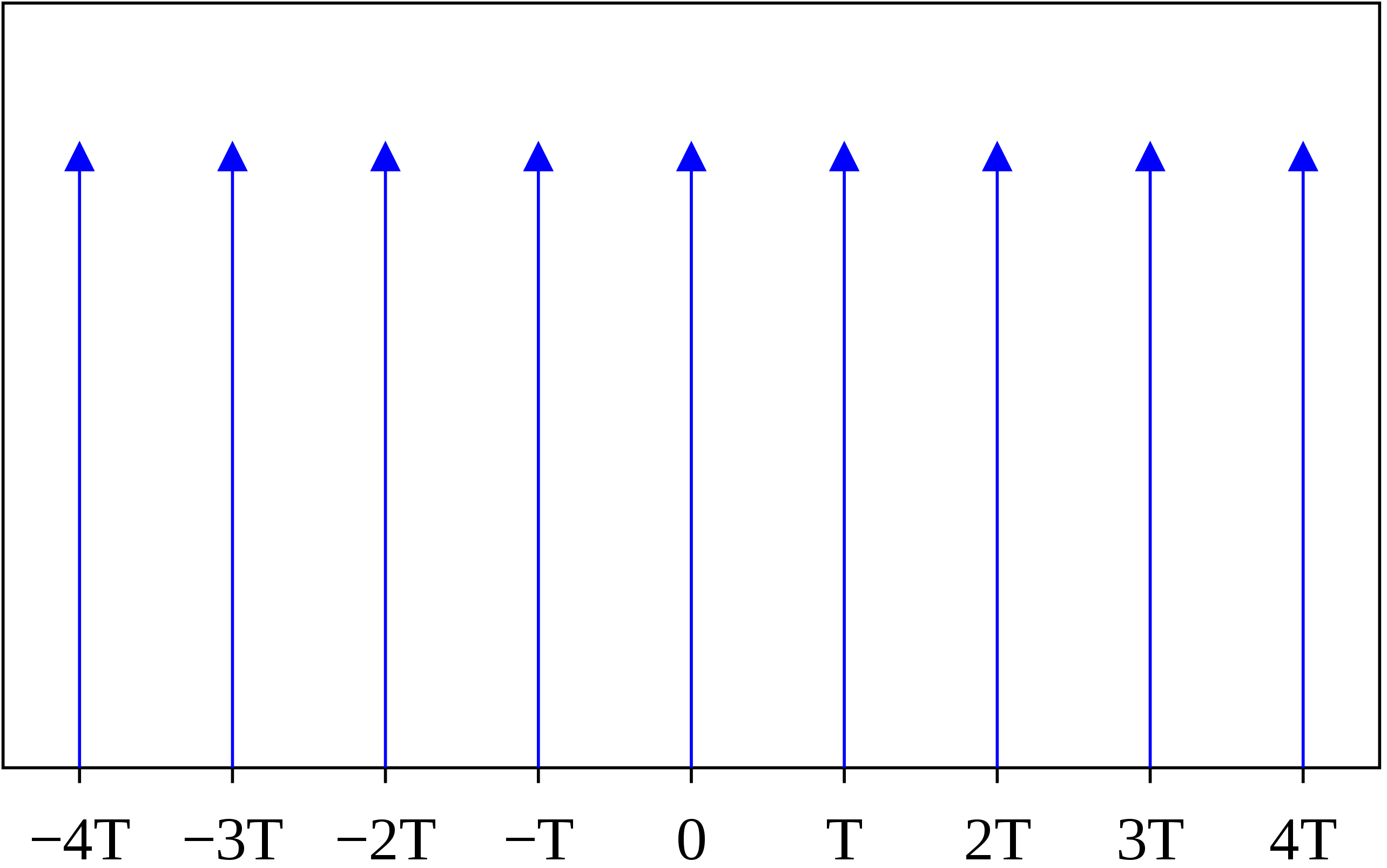
Figure 2: The Dirac comb.

For our purpose it will be sufficient to use a truncated version of the series,

$$V(t)\,=\,\sum_{i=1}^{n}V_{i}\,\delta(t-t_{i}),$$ (93)

where $V_{i}\in\mathbb{R}$ denotes an array of $n$ values. Clearly, the unitarity argument presented in section 2.1 is inadequate for the above choice of Hamiltonian due to the failure of additivity at the singular times $t_{i}$. Let us now examine the resulting expansion from the Dyson series. With the aid of the integration in eq. (36), one finds the following expressions for eqs. (LABEL:unita) and (LABEL:exppnor):

$$\begin{split}&U(t,\,0)\,=\,1\,-\,i\sum_{i=1}^{n}V_{i}\,\Theta(t-t_{i})\,-\,\sum_{i=1}^{n}V_{i}^{2}\,\int_{0}^{t}dt^{\prime}\,\delta(t^{\prime}-t_{i})\,\Theta(t^{\prime}-t_{i})\,+\,\ldots\\ &\mathcal{N}(t,\,0)\,=\,1\,-\,\frac{1}{2}\left(\sum_{i=1}^{n}V_{i}\,\Theta(t-t_{i})\right)^{2}\,+\,\sum_{i=1}^{n}V_{i}^{2}\,\int_{0}^{t}dt^{\prime}\,\delta(t^{\prime}-t_{i})\,\Theta(t^{\prime}-t_{i})\,+\,\ldots\end{split}$$ (94)

As expected, based on the discussion in 2.3, both the results for $U$ and $\mathcal{N}$ above are ill-defined due to the last term (which cancels when taking their products.) Therefore, one can think of $\mathcal{N}$ as a regulator which replaces indeterminate integrals of $U$ by valid integrals describing the dynamics in the form of spikes. Just in order to make some plots of how $\mathcal{N}$ evolves, it is useful to introduce the "defined part of $\mathcal{N}$" (denoted by $\mathcal{D}_{\mathcal{N}}$) as the part of $\mathcal{N}$ which does not involve integration over products of distributions,

$$\mathcal{D}_{\mathcal{N}}(t,\,0)\,\equiv\,1\,-\,\frac{1}{2}\left(\sum_{i=1}^{n}V_{i}\,\Theta(t-t_{i})\right)^{2}\,+\,\ldots$$ (95)

A plot of the last expression is shown in fig. 3. We note that if $\mathcal{N}$ was differentiable like an ordinary function, then indeed $\frac{d\mathcal{N}}{dt}=0$, however, $\mathcal{N}$ is non-differentiable. However, the construction defined by $\mathcal{P}(t,\,0)$, as defined by eq. (LABEL:pitarg2), involves the action of $\mathcal{N}(t,\,0)$ on $U(t,\,0)$ before the evaluation of the integrals. One arrives at a result which does not include ill-defined terms,

$$\mathcal{P}(t,\,0)\,=\,\mathcal{N}(t,\,0)\,U(t,\,0)\,=\,1\,-\,i\sum_{i=1}^{n}V_{i}\,\Theta(t-t_{i})\,-\,\frac{1}{2}\left(\sum_{i=1}^{n}V_{i}\,\Theta(t-t_{i})\right)^{2}\,+\,\ldots$$ (96)

To all orders, the complete resummation of the series is given by the Magnus expansion, as in the RHS of (19),

$$\mathcal{P}(t,\,0)\,=\,e^{-\,i\sum_{i=1}^{n}V_{i}\,\Theta(t-t_{i})}.$$ (97)

More explicitly, the result of the above series can also be written as

$$\mathcal{P}(t,\,0)\,=\,\begin{cases}\begin{array}[]{c}1\\ e^{-iV_{1}}\\ \cdots\\ e^{-i\sum_{i=1}^{n}V_{i}}\end{array}&\begin{array}[]{c}0\leq t<t_{1}\\ t_{1}<t<t_{2}\\ \cdots\\ t_{n}<t\end{array}\end{cases}.$$ (98)

Although our formalism does not describe what happens at the isolated transition time $t_{1}$, this is not of any concern. Practically, the time that a perturbation is turned on is well separated from the time that a measurement is conducted.

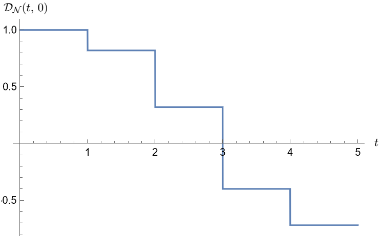
Figure 3: The value of the defined part of $\mathcal{N}(t,\,0)$ for the Dirac comb Hamiltonian (93) with $n=4$ and $V_{i}\,=\,\{0.6,\,1,\,1.2,\,0.8\}$.

We would like to finish this part with a comment. It is tempting to think that the problem with products of distributions can be solved by replacing the Dirac delta function by a function with a finite width $\epsilon>0$. This can be done by using either the nascent or Gaussian representation,

$$\delta(x)\,\rightarrow\,\frac{\epsilon}{\pi(x^{2}+\epsilon^{2})},\qquad\qquad\delta(x)\,\rightarrow\,\frac{1}{2\sqrt{\pi\epsilon}}\exp\left(-\frac{x^{2}}{4\epsilon}\right).$$ (99)

By applying such a replacement one effectively replace an unbounded Hamiltonian with a bounded version, and the description of the system is given entirely by $U(t,\,0)$. However, it is crucial to understand that this demands from us the introduction of an additional dimensionful parameter – the width. Of course, the replaced integrals exist only as long as the width is kept finite, and become indeterminate once the width is vanishing. While the introduction of dimensionful parameter can sometime be justified, a clear advantage is to have an approach that is compatible with the Hamiltonian already in its original form.

4.3 Singular time-independent potentials

In this part we would like to discuss the implication on unitarity for the case of a an unbounded time-independent potential that is localized in space. One of simplest examples that can be chosen in order to study this case is a one dimensional distribution,

$$V(x)\,=\,\alpha\delta(x).$$ (100)

The resulting differential equation governing the time evolution, as given by (1), is

$$i\frac{d}{dt}U(t,\,t_{0})\,=\,\alpha\delta(x)\,U(t,\,t_{0}).$$ (101)

At first sight, we are tempted to write the corresponding evolution operator by plugging the Hamiltonian above inside equation (2),

$$U(t,\,t_{0})\,=\,\exp\left[-i\int_{t_{0}}^{t}dt^{\prime}\,\delta(x)\right]\,=\,\exp\left[-i\Delta t\,\delta(x)\right].$$ (102)

However, result (102) is obtained under the assumption of classical integrability of the RHS of (101), so that the fundamental theorem of calculus applies. In the neighborhood of the singular point, $x=0$, the situation becomes troublesome since no analogous theorem applies for generalized objects. An important observation is that since the Taylor series expansion does not exist in the neighborhood of the singular point, one cannot repeat the considerations of (46). Therefore, without getting into the details of how to define the exponentiation of a generalized object, we conclude that formally

$$\left(\exp\left[-i\Delta t\,\delta(x)\right]\right)^{\dagger}\,\neq\,\left(\exp\left[-i\Delta t\,\delta(x)\right]\right)^{-1}.$$ (103)

Meaning that (102) cannot be regarded as a unitary operator on the entire space. Under the understanding of (103), we can use the following formal structure as a unitary operator

$$\mathcal{P}(t,\,t_{0})\,=\,\sqrt{\exp^{\dagger-1}\left[-i\Delta t\,\delta(x)\right]\,\exp^{-1}\left[-i\Delta t\,\delta(x)\right]}\exp\left[-i\Delta t\,\delta(x)\right].$$ (104)

Clearly, similar situation will occur for other familiar singular potentials, such as the Coulomb and Yukawa potentials, given by $V(r)\,=\,\frac{1}{r}$ and $V(r)\,=\,\frac{e^{-\mu r}}{r}$ respectively.

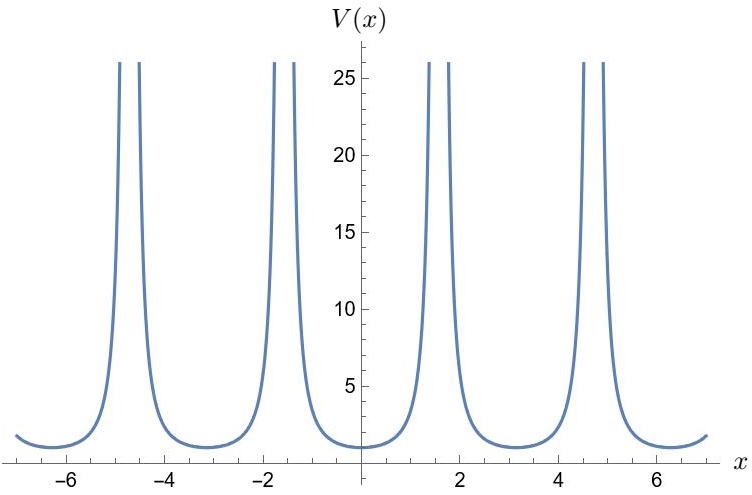
Figure 4: The Poschl-Teller potential with $V_{0}=\alpha=1$.

The situation becomes more interesting when passing from potentials with only a single singular point to the case in which a measure-$0$ set of singularities is involved. An explicit example for such a potential is the Poschl-Teller potential (see fig.4),

$$V(\hat{x})\,=\,\frac{V_{0}}{\cos^{2}\alpha\hat{x}},$$ (105)

which after extracting the generalized part can be written

$$\lim_{\epsilon\rightarrow 0}\frac{V_{0}}{\cos^{2}\alpha\hat{x}-i\epsilon}\,=\,P.v.\left(\frac{V_{0}}{\cos^{2}\alpha\hat{x}}\right)+i\pi\delta(\cos^{2}\alpha\hat{x}).$$ (106)

Showing us that unitarity is not maintained at the tunneling points. Without solving the singular dynamics, one has to specify itself only for a specific branch of the potential, and cannot realize the entire dynamics that includes the singular locations.

4.4 The harmonic oscillator

In this part we study the case of potential given by the harmonic oscillator on an unbounded phase space. Such a potential is given by

$$\hat{V}(\hat{x})\,=\,\frac{1}{2}m\omega^{2}\hat{x}^{2}.$$ (107)

The result for the corresponding propagator based on $\hat{U}$ is well known Feynman and has been first obtained by Feynman on the basis of discretization of time evolution as in (51),

$$\mathcal{K}(x,x_{0};\,\Delta t)\,=\,\sqrt{\frac{m\omega}{2\pi i\sin(\omega\Delta t)}}\exp\left(\frac{im\omega}{2\sin(\omega\Delta t)}\left[(x_{0}^{2}+x^{2})\cos(\omega\Delta t)-2xx_{0}\right]\right).$$ (108)

Our intention here is to point the problem with unitarity of the above result, and explain why by itself (108) cannot be the complete story. Let us start by reminding the basic definition of the propagator in terms of the position Hilbert space,

$$\hat{U}(t,\,t_{0})\,=\,\mathcal{K}(x,x_{0};\,\Delta t)\left|x\right\rangle\left\langle x_{0}\right|\;;\qquad\qquad\mathcal{K}(x,x_{0};\,\Delta t)\,\equiv\,\left\langle x\right|\hat{U}(t,\,t_{0})\left|x_{0}\right\rangle.$$ (109)

The result above is naturally obtained by introducing the identity operator, $\left|x\right\rangle\left\langle x\right|\,=\,\hat{\bm{1}}$, on both sides of $\hat{U}$ (integration over repeated position kept implicit.) Since the identity involves orthonormal states, unitarity is supposed to be kept unchanged by the new representation as

$$\hat{U}^{\dagger}(t,\,t_{0})\,\hat{U}(t,\,t_{0})\,=\,\int_{-\infty}^{\infty}dx\,dx_{1}\,dx_{0}\,\left|x\right\rangle\mathcal{K}^{*}(x_{1},x;\,\Delta t)\,\mathcal{K}(x_{1},x_{0};\,\Delta t)\left\langle x_{0}\right|.$$ (110)

In terms of the propagator the necessary condition for unitarity translates directly to

$$I\,\equiv\,\int_{-\infty}^{\infty}dx_{1}\,\mathcal{K}^{*}(x_{1},x;\,\Delta t)\,\mathcal{K}(x_{1},x_{0};\,\Delta t)\,=\,\delta(x-x_{0})\,.$$ (111)

The relation above must hold for any given value of $\Delta t$, as only in that case

$$\hat{U}^{\dagger}(t,\,t_{0})\,\hat{U}(t,\,t_{0})\,=\,\int_{-\infty}^{\infty}dx\,dx_{0}\,\left|x\right\rangle\delta(x-x_{0})\left\langle x_{0}\right|\,=\,\int_{-\infty}^{\infty}dx\,\left|x\right\rangle\left\langle x\right|\,=\,\hat{\bm{1}}.$$ (112)

The resulting condition from the LHS of (111) after insertion of (108) seems to be

$$\begin{split}I\,=\,\frac{m\omega}{2\pi\sin(\omega\Delta t)}\int_{-\infty}^{\infty}dx_{1}\exp\left(\frac{im\omega}{2\sin(\omega\Delta t)}\left[(x_{0}^{2}-x^{2})\cos(\omega\Delta t)+2x_{1}(x-x_{0})\right]\right).\end{split}$$ (113)

In the current approach, the fulfillment of the condition in (111) of the above result is based on using the simplification

$$\frac{m\omega}{2\pi\sin(\omega\Delta t)}\int_{-\infty}^{\infty}dx_{1}\exp\left(\frac{im\omega}{\sin(\omega\Delta t)}x_{1}(x-x_{0})\right)\,=\,\delta(x-x_{0}),$$ (114)

in addition to

$$f(x)\,\delta(x-x_{0})\,=\,f(x_{0})\,\delta(x-x_{0}).$$ (115)

However, the last simplifications cannot always be done. The assumption behind the simplification (115) is that the argument of the $f(x)$ is a bounded function (see appendix C,) which is correct only for times where $\sin(\omega\Delta t)\,\neq\,0$. During the measure-$0$ singular times when $\sin(\omega\Delta t)=0$, or equivalently $\Delta t\,=\,\frac{\pi n}{\omega}$ with $n\in\mathbb{Z}$, expression (113) is not integrable and the expression obtains a meaning only in the generalized sense. This problem was, in fact, previously identified in Souriau , suggesting to replace the familiar result (108) with an alternative one:

$$\begin{split}&\mathcal{K}_{s}(x,x_{0};\,\Delta t)\\ &=\begin{cases}\begin{array}[]{c}\sqrt{\frac{m\omega}{2\pi i\left|\sin(\omega\Delta t)\right|}}\exp\left(-\frac{i\pi}{2}\left[\frac{\omega\Delta t}{\pi}\right]\right)\exp\left(\frac{im\omega}{2\sin(\omega\Delta t)}\left[(x_{0}^{2}+x^{2})\cos(\omega\Delta t)-2xx_{0}\right]\right)\\ \exp\left(-\frac{i\pi}{2}n\right)\,\delta(x-(-1)^{n}x_{0})\end{array}\end{cases},\end{split}$$ (116)

where the upper result applies for $\Delta t$ such that $\sin(\omega\Delta t)=0$, while the lower one for $\Delta t$ such that $\sin(\omega\Delta t)\neq 0$. This modified version allows to provide some meaning for the description of the propagator at the turning-points. However, this suffers from other problems such as discontinuity as a result of using the floor function.

Now let us compute the result for the propagator that is obtained based on $\mathcal{\hat{P}}$. The new propagator is denoted in analogy to (109) via $\hat{\mathcal{P}}=\mathcal{\widetilde{K}}(x,x_{0};\,\Delta t)\left|x\right\rangle\left\langle x_{0}\right|,$ where

$$\begin{split}&\mathcal{\widetilde{K}}(x,x_{0};\,\Delta t)\,\equiv\,\left\langle x\right|\hat{\mathcal{N}}(t,\,t_{0})\left|x_{1}\right\rangle\left\langle x_{1}\right|\hat{U}(t,\,t_{0})\left|x_{0}\right\rangle\,=\,\mathcal{N}(x,x_{1};\,\Delta t)\,\mathcal{K}(x_{1},x_{0};\,\Delta t).\end{split}$$ (117)

In the result above the following definition is introduced:

$$\mathcal{N}(x,x_{1};\,\Delta t)\,\equiv\,\left\langle x\right|\sqrt{\left(\mathcal{K}^{*}(y_{1},y;\,\Delta t)\,\mathcal{K}(y_{1},y_{0};\,\Delta t)\left|y\right\rangle\left\langle y_{0}\right|\right)^{-1}}\left|x_{1}\right\rangle.$$ (118)

The quantity above can be computed based on (108) keeping in mind the need to avoid invalid simplifications as mentioned in footnote 40. Clearly, the new propagator is manifestly unitary without even the need to compute any integrals,

$$\begin{split}&\mathcal{\widetilde{K}}^{*}(x_{2},x;\,\Delta t)\,\mathcal{\widetilde{K}}(x_{2},x_{0};\,\Delta t)\,\\ &=\left\langle x\right|\hat{U}^{\dagger}(t,\,t_{0})\left|x_{3}\right\rangle\left\langle x_{3}\right|\hat{\mathcal{N}}(t,\,t_{0})\left|x_{2}\right\rangle\left\langle x_{2}\right|\hat{\mathcal{N}}(t,\,t_{0})\left|x_{1}\right\rangle\left\langle x_{1}\right|\hat{U}(t,\,t_{0})\left|x_{0}\right\rangle=\left\langle x\left|x_{0}\right.\right\rangle,\end{split}$$ (119)

analogously to (22).

4.5 Why do we really need to normalize the WF?

In this part we demonstrate the implications of the new solution on calculations that involve gauge theories using old fashioned perturbation theory. In the first example, we explain why the only justification for normalizing the WF must come directly from the solution itself. In the second example, we discuss an experimental setup that can be used to confirm the suggested solution by using entangled scattering. In this example, we compute the wave-function of an electron assuming QED as our gauge theory. This computation can be found in the literature (see, for example, adhoc .) However, while the current approach allows to find the correct final result, we would like to show that it relies on intermediate mathematical steps which are unjustified and fail to work in more general situations. Our initial electron $\left|e^{-}\right\rangle$ is prepared on-shell at $t_{0}=-\infty$ with a fixed energy $E_{e^{-}}$, and its bare WF is properly normalized. Since we specify ourselves to order $\alpha_{e.m.}$, the electron can only evolve by interacting with itself via the emission and absorption of a photon until the evolution terminates at $t=0$. As the complete Fock space is spanned by the space of $\left\{\left|e^{-}\,\gamma\right\rangle,\,\left|e^{-}\right\rangle\right\}$, the Fock identity (153) becomes

$$\int d\Pi_{e^{-}}\left|e^{-}\right\rangle\left\langle e^{-}\right|\,+\,\int d\Pi_{e^{-}\gamma}\left|e^{-}\gamma\right\rangle\left\langle e^{-}\gamma\right|\,+\,\ldots\,=\,\hat{\mathbf{1}},$$ (120)

The expansion for $\hat{U}$ landau , therefore, can be written (keeping the limits $\epsilon\rightarrow 0$ implicit)

$$\begin{split}&\hat{U}(0,-\infty)\left|e^{-}\right\rangle\,=\,\left(\hat{\mathbf{1}}-\int d\Pi_{e_{2}^{-}\gamma,e_{1}^{-}}\left|e_{2}^{-}\gamma\right\rangle\frac{\left\langle e_{2}^{-}\gamma\right|\hat{H}_{int}\left|e_{1}^{-}\right\rangle}{E_{e_{2}^{-}\gamma}-E_{e_{1}^{-}}-i\epsilon}\left\langle e_{1}^{-}\right|\right.\\ &\qquad\qquad\;\;\left.-\int d\Pi_{e_{2}^{-},e_{3}^{-}\gamma,e_{1}^{-}}\left|e_{2}^{-}\right\rangle\frac{\left\langle e_{2}^{-}\right|\hat{H}_{int}\left|e_{3}^{-}\gamma\right\rangle\left\langle e_{3}^{-}\gamma\right|\hat{H}_{int}\left|e_{1}^{-}\right\rangle}{(E_{e_{2}^{-}}-E_{e_{1}^{-}}-i\epsilon_{2})(E_{e_{3}^{-}\gamma}-E_{e_{1}^{-}}-i\epsilon_{1})}\left\langle e_{1}^{-}\right|\right)\left|e^{-}\right\rangle.\end{split}$$ (121)

The complete Hamiltonian, $\hat{H}\,=\,\hat{H}_{0}+\hat{H}_{int}$ consists of two parts – the free field,

$$\hat{H}_{0}\,=\,\frac{\bm{\hat{p}}^{2}}{2m},$$ (122)

with $\hat{H}_{0}\left|e^{-}\right\rangle=E_{e^{-}}\left|e^{-}\right\rangle$ and $\hat{H}_{0}\left|e^{-}\gamma\right\rangle=E_{e^{-}\gamma}\left|e^{-}\gamma\right\rangle$. In addition, to Yukawa’s interaction:

$$\hat{H}_{int}\,\sim\,\int d\Pi_{P_{2},P_{1},K_{1}}\,\delta(P_{2}+P_{1}-K_{1})\,\mathcal{V}(P_{2},\,K_{1})\,a^{\dagger}(P_{2})\,b^{\dagger}(P_{1})\,b(K_{1})\,+\,(c.c)\,.$$ (123)

with $\mathcal{V}=\mathcal{V}(P_{2},\,K_{1})$ denoting the vertex factor, $b^{\dagger}(P_{1})$ and $b(K_{1})$ denoting the creation and annihilation operators of a quark state, and $a^{\dagger}(P_{2})$ denoting the creation operator of a photon. The last structure directly leads to

$$\left\langle e_{2}^{-}(p_{1})\,\gamma(p_{2})\right|\hat{H}_{int}\left|e_{1}^{-}(k_{1})\right\rangle\,\sim\,\mathcal{V}(p_{2},\,k_{1})\,\delta(p_{1}+p_{2}-k_{1}),$$ (124)

and after combining with the additional matrix element,

$$\begin{split}&\left\langle e_{2}^{-}(k_{2})\right|\hat{H}_{int}\left|e_{3}^{-}(p_{1})\,\gamma(p_{2})\right\rangle\left\langle e_{3}^{-}(p_{1})\,\gamma(p_{2})\right|\hat{H}_{int}\left|e_{1}^{-}(k_{1})\right\rangle\\ &\sim\,\mathcal{V}^{*}(p_{2},\,k_{1})\,\mathcal{V}(p_{2},\,k_{2})\,\delta(p_{1}+p_{2}-k_{2})\,\delta(p_{1}+p_{2}-k_{1}).\end{split}$$ (125)

The the last term of (LABEL:elecwf) points to us on a problem: performing the integrations over the electron momentum after introducing (LABEL:enecon) (which implies that $E_{e_{2}^{-}}=E_{e_{1}^{-}}$) leads to:

$$\int d\Pi_{\gamma}\,\left|e^{-}\right\rangle\frac{|\mathcal{V}|^{2}}{E_{\tilde{e}^{-}\gamma}-E_{e^{-}}}\,\lim_{\epsilon\rightarrow 0}\frac{1}{-i\epsilon}\,.$$ (126)

This term is obviously ill-defined and in the current approach is dropped "by hand" on the basis of combining it with its complex conjugate. Meaning that, since it is assumed to be treated as a pure imaginary number, and the following simplification is taken (at the level of observable,)

$$\lim_{\epsilon\rightarrow 0}\frac{1}{-i\epsilon}+\left(\lim_{\epsilon\rightarrow 0}\frac{1}{-i\epsilon}\right)^{\dagger}\nrightarrow 0.$$ (127)

However, this conclusion is based on an invalid operation of exchanging a limit and a conjugation that is valid only for finite numbers. Mathematically, infinite is not an element of $\mathbb{R}$, and therefore, one cannot apply the conjugation on it in the standard way. Based on the expected irrelevancy of the ill-defined term, a truncated version of (LABEL:elecwf) is introduced known as the dressed electron state (denoted with a subscript $D$,)

$$\left|e^{-}\right\rangle_{D}\,\equiv\,\left.\hat{U}(0,-\infty)\right|_{g}\left|e^{-}\right\rangle\,=\,\left(\hat{\mathbf{1}}-\int d\Pi_{e_{1}^{-},e_{2}^{-}\gamma}\left|e_{2}^{-}\gamma\right\rangle\frac{\left\langle e_{2}^{-}\gamma\right|\hat{H}_{int}\left|e_{1}^{-}\right\rangle}{E_{e_{2}^{-}\gamma}-E_{e_{1}^{-}}-i\epsilon}\left\langle e_{1}^{-}\right|\right)\left|e^{-}\right\rangle.$$ (128)

An immediate observation is that the norm of the asymptotic state has been changed during the evolution process, $\left\|\left|e^{-}\right\rangle_{D}\right\|\,\neq\,\left\|\left|e^{-}\right\rangle\right\|$. The familiar approach to cope with the last problem is by introducing the wave function normalization factor $\mathcal{Z}$ as an overall coefficient, so that $\left|e^{-}\right\rangle_{D}\longrightarrow\mathcal{Z}\left|e^{-}\right\rangle_{D}$ such that

$$\left\|\mathcal{Z}\,\left|e^{-}\right\rangle_{D}\right\|\,=\,\left\|\left|e^{-}\right\rangle\right\|\,.$$ (130)

The value of $\mathcal{Z}$ is dictated by the above constraint:

$$\mathcal{Z}\,=\,1-\frac{1}{2}\int d\Pi_{e_{1}^{-}\gamma}\frac{\left\langle e^{-}\right|\hat{H}_{int}\left|e_{1}^{-}\gamma\right\rangle\left\langle e_{1}^{-}\gamma\right|\hat{H}_{int}\left|e^{-}\right\rangle}{(E_{e_{1}^{-}\gamma}-E_{e^{-}}+i\epsilon_{2})(E_{e_{1}^{-}\gamma}-E_{e^{-}}-i\epsilon_{1})}.$$ (131)

The last result is known as the "self-energy" contribution (fig. 5).

Figure 5: The electron self-energy diagram: an on-shell electron emits a virtual photon and then absorbs it back. This contribution does not exist properly in the expansion for $\hat{U}$, and an additional ad-hoc normalization procedure in required in order to obtain the expression for this contribution.

Finally, the result after the "surgery" becomes

$$\begin{split}&\mathcal{Z}\,\left|e^{-}\right\rangle_{D}\,=\,\left|e^{-}\right\rangle-\int d\Pi_{e_{1}^{-}\gamma}\left|e_{1}^{-}\gamma\right\rangle\frac{\left\langle e_{1}^{-}\gamma\right|\hat{H}_{int}\left|e^{-}\right\rangle}{E_{e_{1}^{-}\gamma}-E_{e^{-}}-i\epsilon}\\ &\,\;\qquad\quad\;\;-\frac{1}{2}\int d\Pi_{e_{1}^{-}\gamma}\left|e^{-}\right\rangle\frac{\left\langle e^{-}\right|\hat{H}_{int}\left|e_{1}^{-}\gamma\right\rangle\left\langle e_{1}^{-}\gamma\right|\hat{H}_{int}\left|e^{-}\right\rangle}{(E_{e_{1}^{-}\gamma}-E_{e^{-}}+i\epsilon_{2})(E_{e_{1}^{-}\gamma}-E_{e^{-}}-i\epsilon_{1})}.\end{split}$$ (132)

At this point the following questions comes to mind – are we really allowed to change the original result ’by hand’? what value does the WF normalization $\mathcal{Z}$ obtain at finite times? After all, it would have been better to arrive at the final result (LABEL:elecwfnor) from first principles, without the need for any additional operations. Surprisingly, the current assumption of QFT formalism assumes that the normalization of the perturbed state does not change at any given finite time ($\mathcal{Z}=1$,) so that $\mathcal{Z}$ suddenly gets its value only at the asymptotic times. However, such an underlying assumption is with an obvious conflict with the principle of homogeneity of time. Clearly, if the normalization factor exist also at the finite times, there is no escape from the conclusion that this factor is, in fact, a part of the solution itself that develops gradually as time goes by. In order to give an answer to the second question above we promote $\mathcal{Z}\>\rightarrow\>\hat{\mathcal{Z}}$ in relation (130), so that

$$\left\|\hat{\mathcal{Z}}\,\left|e^{-}\right\rangle_{D}\right\|\,=\,\left\|\left|e^{-}\right\rangle\right\|\qquad\longrightarrow\qquad\hat{U}^{\dagger}(0,\,-\infty)\,\hat{\mathcal{Z}}^{2}\,\hat{U}(0,\,-\infty)\,=\,\bm{\hat{1}}.$$ (133)

From the last relation, we realize that the operator $\hat{\mathcal{Z}}$ is dictated to be defined as

$$\hat{\mathcal{Z}}\,=\,\sqrt{\hat{U}^{\dagger-1}(0,\,-\infty)\,\hat{U}^{-1}(0,\,-\infty)},$$ (134)

which has the obvious relation to $\hat{\mathcal{N}}$ via

$$\lim_{t_{0}\rightarrow-\infty;\>t\rightarrow 0}\hat{\mathcal{N}}(t,\,t_{0})\,=\,\hat{\mathcal{Z}}.$$ (135)

Indeed, an immediate calculation of (134) leads to

$$\begin{split}&\hat{\mathcal{N}}(0,-\infty)\,=\,\hat{\bm{1}}+\int d\Pi_{\tilde{e}^{-},e^{-}\gamma,e^{-}}\left|\tilde{e}^{-}\right\rangle\frac{\left\langle\tilde{e}^{-}\right|\hat{H}_{int}\left|e^{-}\gamma\right\rangle\left\langle e^{-}\gamma\right|\hat{H}_{int}\left|e^{-}\right\rangle}{(E_{\tilde{e}^{-}}-E_{e^{-}}-i\epsilon_{2})(E_{e^{-}\gamma}-E_{e^{-}}-i\epsilon_{1})}\left\langle e^{-}\right|\\ &\qquad\qquad\;\>\,-\frac{1}{2}\int d\Pi_{\tilde{e}^{-},e^{-}\gamma,e^{-}}\left|\tilde{e}^{-}\right\rangle\frac{\left\langle\tilde{e}^{-}\right|\hat{H}_{int}\left|e^{-}\gamma\right\rangle\left\langle e^{-}\gamma\right|\hat{H}_{int}\left|e^{-}\right\rangle}{(E_{e^{-}\gamma}-E_{\tilde{e}^{-}}+i\epsilon_{2})(E_{e^{-}\gamma}-E_{e^{-}}-i\epsilon_{1})}\left\langle e^{-}\right|.\end{split}$$ (136)

Including the additional operator $\mathcal{\hat{N}}$ as a part of the solution, allows us to get a result that is "ready to go" from the first moment without the need for an additional ad-hoc procedure.

When is normalization not just a simple overall factor?

Short answer: when dealing with an evolved a mixed state. Suppose that we have at hand an initial state $\left|\psi(t_{0})\right\rangle$ expressed by a sum of pure states. Now let us look at look at the case in which a non-trivial norm was developed for the evolved state $\left|\psi(t_{1})\right\rangle\,=\,\hat{U}(t_{1},\,t_{0})\left|\psi(t_{0})\right\rangle$ denoted by $\mathcal{Z}_{\psi}\,\equiv\,\left\|\left|\psi(t_{1})\right\rangle\right\|_{\mathcal{H}}\,\neq\,\left\|\left|\psi(t_{0})\right\rangle\right\|_{\mathcal{H}}$. By using a simple division procedure it is straightforward to obtain a normalized state,

$$\left|\psi(t_{1})\right\rangle\,\longrightarrow\,\frac{1}{\mathcal{Z}_{\psi}}\left|\psi(t_{1})\right\rangle\,=\,\hat{\mathcal{N}}\left|\psi(t_{1})\right\rangle.$$ (137)

Our intention in this part is to motivate the idea that there can be situations in which this simple prescription fails and one must use a generalized procedure carried by an operator. In order to demonstrate how that happens, we explore here the production and evolution of a mixed $e^{-}\,e^{+}$ state. Such is the case when an initial particle evolves, potentially scattered, and then evolves again until being measured. This situation is assumed to be described by the action of subsequent evolution operators triple , $\hat{U}(t_{2},\,t_{1})\,\hat{S}(t_{1})\,\hat{U}(t_{1},\,t_{0})\left|\psi(t_{0})\right\rangle$ with $\hat{S}$ a localized unitary operator that acts at $t_{1}$ (for example, by dressing the scattered partons with Wilson lines.) The scattering itself will be irrelevant for our considerations and can be tuned off by taking the limit $\hat{S}\rightarrow\hat{\bm{1}}$. For convenience, here the asymptotic times are in use: $t_{2}=\infty$, $t_{1}=0$, and $t_{0}=-\infty$. Let our initial state $\left|\psi(t_{0})\right\rangle=\left|\gamma(k)\right\rangle_{t_{0}}$ be a photon with fixed momentum $k$ where the time evolution is generated according to QED Hamiltonian. Our intention here is to explain why there is no possibility of finding scalar $\mathcal{Z}$ that satisfies the condition as in (137),

$$\left\|\mathcal{Z}\,\hat{U}(t_{2},\,t_{1})\,\hat{U}(t_{1},\,t_{0})\left|\gamma\right\rangle_{t_{0}}\right\|\,=\,\left\|\left|\gamma\right\rangle_{t_{0}}\right\|,$$ (138)

while nevertheless,

$$\left\|\hat{\mathcal{P}}(t_{2},\,t_{1})\,\hat{\mathcal{P}}(t_{1},\,t_{0})\left|\gamma\right\rangle_{t_{0}}\right\|\,=\,\left\|\left|\gamma\right\rangle_{t_{0}}\right\|.$$ (139)

Similar to what we saw in (128), the evolution during $t_{0}\rightarrow t_{1}$ of the initial photon state is given by

$$\left|\gamma(k)\right\rangle_{t_{1}}\,=\,\left|\gamma(k)\right\rangle_{t_{0}}\,-\,\int d\Pi_{p}\,\frac{\mathcal{V}_{\gamma\rightarrow e^{-}e^{+}}(k,\,p)}{E_{e^{-}e^{+}}-E_{\gamma}}\left|e^{-}(k-p)\,e^{+}(p)\right\rangle.$$ (140)

Now lets forget about the initial production story and focus on normalizing the mixed state after evolving during $t_{1}\rightarrow t_{2}$ (one can also produce mixed states in alternative ways,)

$$\left|\Phi(k)\right\rangle\,\equiv\,\int d\Pi_{p}\,\phi(k,\,p)\left|e^{-}(k-p)\,e^{+}(p)\right\rangle.$$ (141)

                  

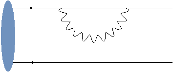
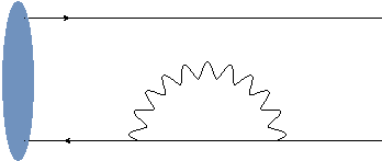
Figure 6: The self-energy diagrams: an electron (or positron) emits a virtual photon and then absorbs it back. This contribution does not exist properly in the expansion for $\hat{U}$, and an additional normalization procedure in required in order to obtain the expression for this contribution via $\mathcal{Z}_{e^{-}}$ and $\mathcal{Z}_{e^{+}}$.

Naively, one might expect the normalization procedure (137) to be generalized by the replacement

$$\hat{U}(t_{2},\,t_{1})\left|\Phi(k)\right\rangle\,\longrightarrow\,\frac{1}{\mathcal{Z}_{e^{+}}\mathcal{Z}_{e^{-}}}\hat{U}(t_{2},\,t_{1})\left|\Phi(k)\right\rangle,$$ (142)

with $\mathcal{Z}_{e^{-}}\,\equiv\,\left\|\hat{U}(\infty,0)\left|e^{-}(k-p)\right\rangle\right\|$ and $\mathcal{Z}_{e^{+}}\,\equiv\,\left\|\hat{U}(\infty,0)\left|e^{+}(p)\right\rangle\right\|$.

It can be shown that the the prescription (142) indeed manages to generate some of the necessary contributions (see fig. 6.) However, the action of $\mathcal{\hat{N}}$ generates additional contributions that involve an internal exchange between the particles given by a convolution that is not of the form of (142) (see fig. 7,)

$$\mathbf{\mathcal{\hat{N}}}(t_{2},\,t_{1})\,\hat{U}(t_{2},\,t_{1})\left|\Phi(k)\right\rangle\,\neq\,\frac{1}{\mathcal{Z}_{e^{+}}\mathcal{Z}_{e^{-}}}\hat{U}(t_{2},\,t_{1})\left|\Phi(k)\right\rangle,$$ (143)

These type of states allow an immediate confirmation in favor of the necessary to introduce $\hat{\mathcal{N}}$ as a dynamical part of the solution. Both inclusive and diffractive forward dijet production iancu in $eA$, $pA$, or $\gamma+jet$ experiments can serve for such a demonstration. These important calculations deserve a separate publication and will not be pursued here.

                  

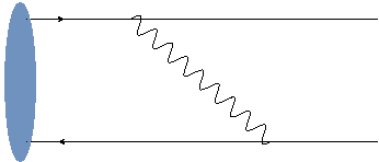
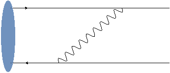
Figure 7: The vertex diagrams: an electron (or positron) emits a photon which is absorbed by the positron (or electron.) This contribution does not exist properly in the expansion for $\hat{U}$ and cannot be generated by introducing an additional overall normalization factor. The action of $\mathcal{\hat{N}}$ generates these contributions.

5 Conclusions

"A harmful truth is better than a useful lie," T. Mann.

The implications of adopting (5) as the new exact solution for the Schrödinger equation are far reaching, and various fundamental aspects of our current understanding of the quantum phenomena are affected. Among the main implications are:

$\circledast$ The currently widely used solution $\hat{U}$ is only a conditionally unitary operator, and is incapable of providing a unitary description for unbounded or non–Hermitian Hamiltonians.

$\circledast$ At the fundamental level, the dynamics of quantum systems is generally non-Markovian. The rigorous mathematical framework to study the singular quantum phenomena naturally involves tools developed in functional analysis and measure theory.

$\circledast$ The Liouville part of the evolution is dormant for bounded Hamiltonians and become activated for unbounded Hamiltonians on a measure 0 set of times of the evolution. It acts as a "probability conservation regulator," and produces a correction for the discontinuous evolution that is involved in the dynamics of $\hat{U}$.

$\circledast$ For the proposed solution unitary is maintained manifestly, at all orders and at any given moment of the evolution, rather than asymptotically. The ordinary probabilistic interpretation is applicable even for unbounded Hamiltonians: the modulus of transitions amplitudes are always given by a defined expressions (up to regularization).

$\circledast$ The current approach of QFT is inconsistent with the principle of homogeneity of time: it assumes that the normalization (or LSZ) factor suddenly appears only for the asymptotic states, without an analogous procedure for the finite times.

$\circledast$ The solution provided will hopefully pave the way for a better understanding of various quantum systems in which unitarity is currently assumed to be broken. As such are systems with a non-Hermitian Hamiltonians, field theories on non-commutative spaces Gomis , field theories on factional dimensions Rychkov , or open quantum systems open .

$\circledast$ The reason which has initiated this study and was not mentioned is the collinear limit, in which the positions of two partons are approaching a common position. Under this limit, as an example, one should not be able to distinguish a system of electron from a system of electron and a photon. $\hat{U}$ can be shown to perturbativly violate this fundamental property, while for $\hat{\mathcal{P}}$ it is preserved (that might be discussed in another paper.) An alternative way of expressing the last statement is that the JIMWLK equation jimwlk describes the high-energy limit behavior of amplitudes, and not only of cross sections.

$\circledast$ Based on the analysis in this paper, we call for measurements in which the procedure of introducing the WF normalization via simple overall $\mathcal{Z}$ factor breaks down. The analysis of the evolution of mixed states should reveal a significant deviation between the theoretical cross sections predictions based on $\hat{U}$ and the actual experimental measurements.

Appendix A The dynamics of $\hat{\mathcal{N}}$

In this part we provide the proof for the second equation of (LABEL:twoeqs). From the defining relation for the normalization operator, $\hat{U}^{\dagger}(t,\,t_{0})\,\mathcal{\hat{N}}^{2}(t,\,t_{0})\,\hat{U}(t,\,t_{0})\,=\,\mathbf{\hat{1}}$. By applying the time derivative on the two side of this equation it follows that

$$\begin{split}&\hat{U}^{\dagger}(t,\,t_{0})\,\left(\mathcal{\hat{N}}(t,\,t_{0})\frac{d\mathcal{\hat{N}}(t,\,t_{0})}{dt}\,+\,\frac{d\mathcal{\hat{N}}(t,\,t_{0})}{dt}\mathcal{\hat{N}}(t,\,t_{0})\right)\,\hat{U}(t,\,t_{0})\\ &=\,-\frac{d\hat{U}^{\dagger}(t,\,t_{0})}{dt}\,\mathcal{\hat{N}}^{2}(t,\,t_{0})\,\hat{U}(t,\,t_{0})\,-\,\hat{U}^{\dagger}(t,\,t_{0})\,\mathcal{\hat{N}}^{2}(t,\,t_{0})\,\frac{d\hat{U}(t,\,t_{0})}{dt}.\end{split}$$ (144)

After multiplication by $\hat{U}^{\dagger-1}(t,\,t_{0})$ from the right side and $\hat{U}^{-1}(t,\,t_{0})$ from the left side becomes

$$\begin{split}&\mathcal{\hat{N}}(t,\,t_{0})\frac{d\mathcal{\hat{N}}(t,\,t_{0})}{dt}\,+\,\frac{d\mathcal{\hat{N}}(t,\,t_{0})}{dt}\mathcal{\hat{N}}(t,\,t_{0})\\ &=\,-\hat{U}^{\dagger-1}(t,\,t_{0})\,\frac{d\hat{U}^{\dagger}(t,\,t_{0})}{dt}\,\mathcal{\hat{N}}^{2}(t,\,t_{0})\,-\,\mathcal{\hat{N}}^{2}(t,\,t_{0})\,\frac{d\hat{U}(t,\,t_{0})}{dt}\,\hat{U}^{-1}(t,\,t_{0}),\end{split}$$ (145)

which is a Sylvester type equation Sylvester for $\frac{d\mathcal{\hat{N}}(t,\,t_{0})}{dt}$. In our case, due to positive definite property of $\mathcal{\hat{N}}$, this equation can be solved in a unique manner. In fact, this equation is not just a Sylvester equation, but more precisely the continuous time Lyapunov equation Lyapunov . As such, its solution is known to be given explicitly by the integral

$$\begin{split}&\frac{d\mathcal{\hat{N}}(t,\,t_{0})}{dt}\,=\,-\int_{0}^{\infty}dy\,e^{-y\mathcal{\hat{N}}(t,\,t_{0})}\\ &\times\left(\hat{U}^{\dagger-1}(t,\,t_{0})\,\frac{d\hat{U}^{\dagger}(t,\,t_{0})}{dt}\,\mathcal{\hat{N}}^{2}(t,\,t_{0})\,+\,\mathcal{\hat{N}}^{2}(t,\,t_{0})\,\frac{d\hat{U}(t,\,t_{0})}{dt}\,\hat{U}^{-1}(t,\,t_{0})\right)e^{-y\mathcal{\hat{N}}(t,\,t_{0})}.\end{split}$$ (146)

By plugging relations (70) in the above result we obtain

$$\begin{split}&\frac{d\mathcal{\hat{N}}(t,\,t_{0})}{dt}\,=\,-\int_{0}^{\infty}dy\,e^{-y\mathcal{\hat{N}}(t,\,t_{0})}\\ &\times\left(i\left(\hat{\mathcal{H}}(t)+i\mathcal{\hat{J}}(t)\right)\,\mathcal{\hat{N}}^{2}(t,\,t_{0})\,-\,i\mathcal{\hat{N}}^{2}(t,\,t_{0})\,\left(\hat{\mathcal{H}}(t)-i\mathcal{\hat{J}}(t)\right)\right)e^{-y\mathcal{\hat{N}}(t,\,t_{0})},\end{split}$$ (147)

which after simplifications can equivalently written

$$\frac{d\mathcal{\hat{N}}(t,\,t_{0})}{dt}=-\int_{0}^{\infty}dy\,\frac{d}{dy}\left[e^{-y\mathcal{\hat{N}}(t,t_{0})}\left(-i\left[\hat{\mathcal{H}}(t),\mathcal{\hat{N}}(t,t_{0})\right]+\mathcal{\hat{N}}(t,\,t_{0})\,\mathcal{\hat{J}}(t)\right)e^{-y\mathcal{\hat{N}}(t,t_{0})}\right].$$ (148)

Finally, an immediate integration of the last result establishes the fact that $\mathcal{\hat{N}}(t,\,t_{0})$ has a non-trivial dynamics that is given by the second equation that is written in (LABEL:twoeqs).

Appendix B The singular perturbative expansion

In this technical part, which can be avoided in first reading, we compute explicitly the perturbative expansion for the asymptotic evolution operator $\mathcal{\hat{P}}(0,\,-\infty)$. Our approach is based on expression (LABEL:pitarg2) and assumes an Hermitian Hamiltonian that is potentially unbounded. Formally, the main idea is to identify a small parameter $g$ such that a series of the following type is obtained

$$\mathcal{\hat{P}}(0,\,-\infty)\,=\,\mathbf{\hat{1}}\,+\,g\hat{I}_{1}\,+\,g^{2}\hat{I}_{2}\,+\,\ldots$$ (149)

with $\left\|g\hat{I}_{1}\right\|\,<\,\left\|g^{2}\hat{I}_{2}\right\|\,<\,\ldots\>$.

The current approach that appears in the literature has an underlying assumption of dealing with the case that no energy levels crossing are involved in the spectrum. So that the eigenvalue of the intermediate states $j$ differs from that of the initial state $i$, $E_{j}\neq E_{i}$. It is customary to add $i\epsilon$ prescription Hannesdottir with the belief that this may allows to extend the validity of the original expansion to the crossing region. However, this prescription is often introduced without additional unjustified assumption that some limit, that we soon will encounter, are iterative. Our intention here is to drop this assumption, and extend the formalism to the singular case in which the energy levels can cross each other.

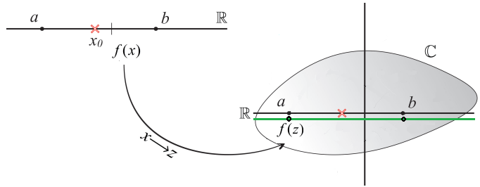
Figure 8: Our original intention was to compute the segment integral of the function $f(x)\in\mathbb{R}$ on the interval $[a,b]\in\mathbb{R}$. Due to a pole at $a<x_{0}<b$, this could not be completed directly. By using complexification, replacing $f(x)\longrightarrow f(z)\in\mathbb{C}$, one generalize the original integration (now on the green line.) The original result can be found taking a singular limit.

The idea is to replace the original differential equation (3) with a modified one, involving a more general class of complex deformed Hamiltonians (see fig. 8). While the original Hamiltonian $\hat{H}(t)$ is producing indeterminate integrations, the last generalization allows us to obtain a non-singular integration, and retaining to the original Hamiltonian can be done by setting a vanishing deformation parameter. From its definition, it is clear the the deformation parameter has to be taken to $0$ as soon as this become possible. A valuable theorem in that respect is given by the Sokhotski–Plemelj theorem:

$$\lim_{\epsilon\rightarrow 0}\frac{1}{x\pm i\epsilon}\,=\,\lim_{\epsilon\rightarrow 0}\frac{x\mp i\epsilon}{x^{2}+\epsilon^{2}}\,=\,P.v.\frac{1}{x}\mp i\pi\delta(x).$$ (150)

As a matter of fact, explicit calculation shows that the new construction for $\mathcal{\hat{P}}$ differs from that of $\hat{U}$. Let us summarize some of properties that can be recognized:

$\bullet$ The first order term
The first order term in the perturbative expansion of (LABEL:pitarg2) reads

$$\hat{I}_{1a}(t,\,t_{0})\,\equiv\,-\frac{i}{2}\int_{t_{0}}^{t}dt^{\prime}\,\hat{H}(t^{\prime},\bm{p}),$$ (151)

and when working with the asymptotic times becomes

$$\hat{I}_{1a}(0,\,-\infty)\,=\,-\frac{i}{2}\int_{-\infty}^{0}dt^{\prime}\,\hat{H}(t^{\prime},\bm{p}).$$ (152)

We introduce a complete Fock space identity of the unperturbed states for the initial and final configurations,

$$\left|i\right\rangle\left\langle i\right|\,=\,\left|i_{1}\right\rangle\left\langle i_{1}\right|\,+\,\left|i_{1},i_{2}\right\rangle\left\langle i_{1},i_{2}\right|\,+\,\ldots\,+\,\left|i_{1},i_{2},\ldots,i_{n}\right\rangle\left\langle i_{1},i_{2},\ldots,i_{n}\right|,$$ (153)

where $\left|i_{1},i_{2},\ldots,i_{n}\right\rangle\left\langle i_{1},i_{2},\ldots,i_{n}\right|$ is integrated over the Hilbert space of $n$ partons. Then

$$\hat{H}(t,\bm{p})\,=\,e^{i\hat{H}_{0}(\bm{p})t}\,\hat{H}(\bm{p})\,e^{-i\hat{H}_{0}(\bm{p})t},$$ (154)

and after denoting the eigenvalues of the Hamiltonian $\hat{H}_{0}(\bm{p})$ by $E_{i}$, such that $\hat{H}_{0}(\bm{p})\left|i\right\rangle=E_{i}\left|i\right\rangle$, we arrive at

$$\hat{I}_{1a}(0,\,-\infty)\,=\,-\frac{i}{2}\int_{-\infty}^{0}dt^{\prime}\,\int d\Pi_{f,i}\,e^{i(E_{f}-E_{i})t^{\prime}}\left|f\right\rangle\left\langle f\right|\hat{H}(\bm{p})\left|i\right\rangle\left\langle i\right|.$$ (155)

The last result might potentially be indeterminate if the spectrum of $i$ and $f$ contain overlapping eigenvalues. It is, therefore, natural to deform the original Hamiltonian in a way that allows us to deviate from hitting these singular occasions on the real line by introducing a complex deformation,

$$\hat{I}_{1a}(0,\,-\infty)\,=\,-\frac{i}{2}\int_{-\infty}^{0}dt^{\prime}\,\int d\Pi_{f,i}\,\lim_{\epsilon\rightarrow 0}e^{i(E_{f}-E_{i}-i\epsilon)t^{\prime}}\left|f\right\rangle\left\langle f\right|\hat{H}(\bm{p})\left|i\right\rangle\left\langle i\right|.$$ (156)

The time integration commutes with both the small deformation limit, as well as the phase space integration,

$$\left[\int_{-\infty}^{0}dt^{\prime},\,\lim_{\epsilon\rightarrow 0}\right]\,=\,\left[\int_{-\infty}^{0}dt^{\prime},\,\int d\Pi_{f,i}\right]=0.$$ (157)

Then, after dragging the time integration to be the first operation,

$$\hat{I}_{1a}(0,\,-\infty)\,=\,-\frac{i}{2}\int d\Pi_{f,i}\,\lim_{\epsilon\rightarrow 0}\int_{-\infty}^{0}dt^{\prime}\,e^{i(E_{f}-E_{i}-i\epsilon)t^{\prime}}\left|f\right\rangle\left\langle f\right|\hat{H}(\bm{p})\left|i\right\rangle\left\langle i\right|.$$ (158)

Performing the integration over $t^{\prime}$ leads to

$$\hat{I}_{1a}(0,\,-\infty)\,=\,-\frac{1}{2}\int d\Pi_{f,i}\,\lim_{\epsilon\rightarrow 0}\frac{1}{(E_{f}-E_{i}-i\epsilon)}\left|f\right\rangle\left\langle f\right|\hat{H}(\bm{p})\left|i\right\rangle\left\langle i\right|.$$ (159)

After using theorem (150), one arrives at the expression

$$\hat{I}_{1a}(0,\,-\infty)\,=\,-\frac{1}{2}\int d\Pi_{f,i}\,\left[P.v.\left(\frac{1}{E_{f}-E_{i}}\right)+i\pi\delta(E_{f}-E_{i})\right]\left|f\right\rangle\left\langle f\right|\hat{H}(\bm{p})\left|i\right\rangle\left\langle i\right|.$$ (160)

So that finally,

$$\hat{I}_{1a}(0,\,-\infty)\,+\hat{I}_{1a}^{\dagger}(0,\,-\infty)=\,-\int d\Pi_{f,i}\,P.v.\left(\frac{1}{E_{f}-E_{i}}\right)\left|f\right\rangle\left\langle f\right|\hat{H}(\bm{p})\left|i\right\rangle\left\langle i\right|.$$ (161)

In typical situations, the above energy denominator involves the creation of an additional parton, creating a hierarchy between the energy differences, $E_{f}\geq E_{i}$. Then, the contribution from the delta function of the above term can be discarded as the additional matrix element (vertex) leads to situation in which the integration is made with respect to $x\delta(x)=0$, and by similar reasoning the principal value can also be removed, leading to

$$\hat{I}_{1a}(0,\,-\infty)\,=\,-\frac{1}{2}\int d\Pi_{f,i}\,\frac{1}{E_{f}-E_{i}}\left|f\right\rangle\left\langle f\right|\hat{H}(\bm{p})\left|i\right\rangle\left\langle i\right|.$$ (162)

$\bullet$ The second order term
At order $g^{2}$, there are five relevant terms in the perturbative expansion for $\mathcal{\hat{P}}$,

$$\begin{split}&\hat{I}_{2}(0,\,-\infty)\,\equiv\,\hat{I}_{2a}(0,\,-\infty)\,-\,3\hat{I}_{2a}^{\dagger}(0,\,-\infty)\,+\,\hat{I}_{2b}(0,\,-\infty)\\ &\qquad\qquad\;\;\>\,+\,\hat{I}_{2c}(0,\,-\infty)\,-\,\hat{I}_{2c}^{\dagger}(0,\,-\infty),\end{split}$$ (163)

where the following definitions are used:

$$\begin{split}&\hat{I}_{2a}(0,\,-\infty)\equiv\frac{1}{8}\left(\int_{-\infty}^{0}dt^{\prime}\>\hat{H}(t^{\prime})\right)^{2},\qquad\hat{I}_{2b}(0,\,-\infty)\equiv-\frac{1}{4}\left|\int_{-\infty}^{0}dt^{\prime}\>\hat{H}(t^{\prime})\right|^{2},\\ &\hat{I}_{2c}(0,\,-\infty)\,\equiv\,-\frac{1}{2}\int_{t_{0}}^{t}dt^{\prime}\hat{H}(t^{\prime})\int_{t_{0}}^{t^{\prime}}dt^{\prime\prime}\hat{H}(t^{\prime\prime}).\end{split}$$ (164)

The result for the first term can be found straightforwardly by a similar reasoning which has led to (160),

$$\begin{split}&\hat{I}_{2a}(0,\,-\infty)\,=\,\frac{1}{8}\int d\Pi_{f,j}\,\left[P.v.\left(\frac{1}{E_{j}-E_{f}}\right)+i\pi\delta(E_{j}-E_{f})\right]\\ &\times\int d\Pi_{i}\,\left[P.v.\left(\frac{1}{E_{j}-E_{i}}\right)+i\pi\delta(E_{j}-E_{i})\right]\left|f\right\rangle\left\langle f\right|\hat{H}(\bm{p})\left|j\right\rangle\left\langle j\right|\hat{H}(\bm{p})\left|i\right\rangle\left\langle i\right|.\end{split}$$ (165)

The contribution $\hat{I}_{2b}(0,\,-\infty)$ of (LABEL:contri) can be found in analogous way to (160). Integration over the time of the remaining contribution leads to

$$\begin{split}&\hat{I}_{2c}(0,\,-\infty)\,=\,-\frac{1}{2}\int d\Pi_{f,j}\,\lim_{\epsilon_{2}\rightarrow 0}\frac{1}{E_{f}-E_{i}-i\epsilon_{2}}\int d\Pi_{i}\,\lim_{\epsilon_{1}\rightarrow 0}\frac{1}{E_{j}-E_{i}-i\epsilon_{1}}\\ &\times\left|f\right\rangle\left\langle f\right|\hat{H}(\bm{p})\left|j\right\rangle\left\langle j\right|\hat{H}(\bm{p})\left|i\right\rangle\left\langle i\right|,\end{split}$$ (166)

so that after using (150) twice,

$$\begin{split}&\hat{I}_{2c}(0,\,-\infty)\,=\,-\frac{1}{2}\int d\Pi_{f,j}\,\left[P.v.\left(\frac{1}{E_{f}-E_{i}}\right)+i\pi\delta(E_{f}-E_{i})\right]\\ &\times\int d\Pi_{i}\,\left[P.v.\left(\frac{1}{E_{j}-E_{i}}\right)+i\pi\delta(E_{j}-E_{i})\right]\left|f\right\rangle\left\langle f\right|\hat{H}(\bm{p})\left|j\right\rangle\left\langle j\right|\hat{H}(\bm{p})\left|i\right\rangle\left\langle i\right|.\end{split}$$ (167)

The result for $\hat{I}_{2}(0,\,-\infty)$ is obtained after combining the above contributions, as required by definition (LABEL:i2def). Our approach is consistent with the work Dumitru . Clearly, in case that no degeneracy is involved in our phase space, for any given $j$, one can performs the replacements

$$P.v.\left(\frac{1}{E_{f}-E_{i}}\right)\longrightarrow\frac{1}{E_{f}-E_{i}},\qquad\qquad\delta(E_{f}-E_{i})\longrightarrow 0.$$ (168)

Meaning, the use of singular perturbation theory is unnecessary, and our approach naturally reduces to regular perturbation theory.

Appendix C How to deal with principal values?

"Singularity is almost invariably a clue," S. Holmes.

The purpose of this part is to show the main advantages of working with principal values with respect to an original integration that contains a singular part. We follow the same definitions as in Hardy’s review on the subject Hardy . For example, $f:\mathbb{R}\setminus a\rightarrow\mathbb{R}$ defined by

$$f(x)\,=\,\frac{1}{x-a}$$ (169)

is a function on the union of two disjoint intervals $(-\infty,\,a)\cup(a,\infty)$, as for any $x$ of these intervals $|f(x)|<\infty$. Obviously, $f(x)$ cannot be regarded as a function for intervals that include the singular point $x=a$. The principal value of $f(x)$ allows us to overcome this problem by introducing a mapping which truncates out the singularities of $f(x)$. Let us suppose that the domain of $f(x)$ possesses a collection of $n$ isolated set of points $X_{1},X_{2},\ldots,X_{n}\in(a,b)$ in which it becomes unbounded, $f(X_{i})=\infty$. The main idea is to define a new construction that allows us to filter out these singularities,

$$P.v.\left(f(x)\right)\,\equiv\,\begin{cases}\begin{array}[]{c}f(x)\\ \lim_{\epsilon_{i}\rightarrow 0}\mathcal{R}e\left(f(x-i\epsilon_{i})\right)\end{array}&\begin{array}[]{c}x\notin\{X_{i}\}\\ x\in\{X_{i}\}\end{array}\end{cases},$$ (170)

where $\{X_{i}\}$ denotes the set of singularities, and $\mathcal{R}e$ denotes the real component which is regraded as bounded. In terms of integrals, the implication of the last definition is that

$$\begin{split}&\int_{a}^{b}P.v.\left(f(x)\right)\,dx\\ &=\,\lim_{\epsilon_{1}\rightarrow 0}\int_{a}^{X_{1}-\epsilon_{1}}f(x)\,dx\,+\,\lim_{\epsilon_{1},\epsilon_{2}\rightarrow 0}\int_{X_{1}+\epsilon_{1}}^{X_{2}-\epsilon_{2}}f(x)\,dx\,+\,\ldots\,+\,\lim_{\epsilon_{n}\rightarrow 0}\int_{X_{n}+\epsilon_{n}}^{b}f(x)\,dx,\end{split}$$ (171)

so that the integration is carried on the interval is $[a,b]/\sum_{i=1}^{n}X_{i}$. The last definition has a great beneficial properties when dealing with singular integrals, as it allows the usage of the familiar manipulations of ordinary functions. For example,

$$\int_{a}^{b}P.v.\left(\frac{x}{x-c}\right)\,dx\,+\,\int_{a}^{b}P.v.\left(\frac{-c}{x-c}\right)\,dx\,=\,b-a,$$ (173)

as long as $f(x)$ is a continuous function,

$$\int_{a}^{b}P.v.\left(\frac{f(x)}{x-d}\right)\,dx\,+\,\int_{b}^{c}P.v.\left(\frac{f(x)}{x-d}\right)\,dx\,=\,\int_{a}^{c}P.v.\left(\frac{f(x)}{x-d}\right)\,dx,$$ (174)

and,

$$\lim_{b\rightarrow a}\int_{a}^{b}P.v.\left(f(x)\right)\,dx\,=\,0.$$ (175)

It is important to understand that the principal value always returns a finite value for any proper integration domain, and may diverge only for improper integration interval. The generalization for higher order of dimensions is natural. By denoting the collection of singulrities of $f(x,y)$ by $\left\{X_{i},Y_{j}\right\}\in(a,b)\times(c,d)$ the following definition is introduced

$$P.v.\left(f(x,y)\right)\,=\,\begin{cases}\begin{array}[]{c}f(x,y)\\ \lim_{\epsilon_{i,j}\rightarrow 0}\mathcal{R}e\left(f(x-i\epsilon_{i},y-i\epsilon_{j})\right)\end{array}&\begin{array}[]{c}(x,y)\notin\left\{X_{i},Y_{j}\right\}\\ (x,y)\in\left\{X_{i},Y_{j}\right\}.\end{array}\end{cases}$$ (176)

For any integration carried on a proper integration interval, the multivariate principal values respect the Fubini theorem:

$$\int_{[a,b]\times[c,d]}P.v.\left(f(x,y)\right)\,dx\,dy\,=\,\int_{[c,d]\times[a,b]}P.v.\left(f(x,y)\right)\,dy\,dx.$$ (177)

The remaining singular part demands a more careful approach and for now we just provide its definition,

$$\int_{[X_{i},Y_{j}]}f(x,y)\,dx\,dy\,=\,\lim_{\varepsilon_{2}\rightarrow 0}\lim_{\varepsilon_{1}\rightarrow 0}\int_{Y_{j}}^{Y_{j}+\varepsilon_{2}}\int_{X_{i}}^{X_{i}+\varepsilon_{1}}f(x,y)\,dx\,dy.$$ (178)

A practical demonstration of the definitions involved in this part is shown in appendix D.

Appendix D Why conditionally convergent integrals fail Fubini?

"Subtle is the lord, but malicious he is not," A. Einstein.

In this part we would like to take a closer look at conditionally convergent integrals and understand what is the exact reason that they may lead to a different results. For the case of infinite series, the fragilness of conditionally convergent sums is well known, and reflected by the Riemann’s series theorem Rudin . For the case of integrals, the theorem which ensures the equivalence of the results obtained with different ordering of integrations is given by the Fubini’s theorem Rudin . There are two ways to avoid satisfying the requirements for Fubini’s theorem singuint – integration of function with an improper domain (first kind), or integration involving a singular point where the distributional limit exists (second kind.)

$\bullet$ First kind

The double improper Riemann integral over an infinite region such as $[0,\infty)^{2}$ is typically defined as

$$\int_{[1,\infty)^{2}}f(x,y)\,dx\,dy\,=\,\lim_{n\to\infty}\int_{A_{n}}f(x,y)\,dx\,dy\,,$$ (179)

where $(A_{n})$ is an increasing sequence of compact, rectifiable sets such that $A_{1}\subset A_{2}\subset\ldots$ and $[0,\infty)^{2}=\cup_{n=1}^{\infty}A_{n}$. That limit can only be uniquely determined independent of the particular sequence $(A_{n})$ when absolute integrability holds. In order to demonstrate this case we choose

$$f(x,\,y)\,\equiv\,\frac{x^{2}-y^{2}}{(x^{2}+y^{2})^{2}},$$ (180)

for which a well-known result is

$$I\,\equiv\,\int_{1}^{\infty}\int_{1}^{\infty}f(x,y)\,dx\,dy\,=\,\frac{\pi}{4}\>,\quad\qquad J\,\equiv\,\int_{1}^{\infty}\int_{1}^{\infty}f(x,y)\,dy\,dx\,=\,-\frac{\pi}{4}.$$ (181)

Since the $f(x,\,y)$ is continuous on $\mathbb{R}^{2}\setminus(0,0)$, it is absolutely integrable over any finite region excluding the point $(0,0)$. Fubini’s theorem guarantees that the iterated integrals must be equal to one another as well as to the double integral as long as proper integration region is involved. That is

$$\int_{1}^{A}\int_{1}^{B}f(x,y)\,dy\,dx\,=\,\int_{1}^{B}\int_{1}^{A}f(x,y)\,dx\,dy\,=\,\int_{[1,A]\times[1,B]}\frac{x^{2}-y^{2}}{(x^{2}+y^{2})}d(x,y)\,,$$ (182)

for any $A,\,B\,<\,\infty$. In order to compute the requested integral on the unbounded domain, let us use the following representations

$$f(x,y)\,=\,-\frac{\partial}{\partial x}\frac{\partial}{\partial y}\arctan\left(\frac{y}{x}\right)\,=\,\frac{\partial}{\partial y}\frac{\partial}{\partial x}\arctan\left(\frac{x}{y}\right).$$ (183)

The meaning of $I$ and $J$ is an iterated limit of integrals over finite intervals $1\leqslant y\leqslant B$ and $1\leqslant x\leqslant A$, where $A$ and $B$ tend independently to $+\infty$. That leads to,

$$\begin{split}&I=\lim_{A\to+\infty}\lim_{B\to+\infty}\int_{1}^{A}\left(\int_{1}^{B}\frac{\partial}{\partial y}\frac{\partial}{\partial x}\arctan\left(\frac{x}{y}\right)\,dy\right)dx=\lim_{A\to\infty}\left(-\arctan A+\frac{\pi}{4}\right)=-\frac{\pi}{4}\,,\end{split}$$ (184)

and similarly,

$$\begin{split}&J=\lim_{B\to+\infty}\lim_{A\to+\infty}\int_{1}^{B}\left(\int_{1}^{A}-\frac{\partial}{\partial x}\frac{\partial}{\partial y}\arctan\left(\frac{y}{x}\right)\,dx\right)\,dy=-\lim_{B\to\infty}\left(-\arctan B+\frac{\pi}{4}\right)=\frac{\pi}{4},\end{split}$$ (185)

showing us that the difference of $\frac{\pi}{2}$ is generated entirely by the asymptotic region.

$\bullet$ Second kind

Now, let us tackle the more tricky part of dealing with the contribution from the singular point. In order to demonstrate how the situation occur let us define the following function $g:\mathbb{R}^{2}\setminus(0,0)\longrightarrow\mathbb{R}$ such that

$$g(x,y)\,=\,\frac{xy(x^{2}-y^{2})}{(x^{2}+y^{2})^{3}}\,.$$ (186)

We would like to show that

$$I\,\equiv\,\int_{0}^{1}\int_{0}^{2}g(x,y)\,dx\,dy\,=\,-\frac{1}{20}\,,\quad\qquad J\,\equiv\,\int_{0}^{2}\int_{0}^{1}g(x,y)\,dy\,dx\,=\,\frac{1}{5}\,.$$ (187)

Let us first decompose $I\,=\,I_{P.v.}+I_{\mathcal{G}}$, by using definitions (176) and (178). The the principal value is obtained easily,

$$I_{P.v.}\,=\,\int_{0}^{1}\int_{0}^{2}P.v.\left(\frac{xy(x^{2}-y^{2})}{(x^{2}+y^{2})^{3}}\right)\,dx\,dy\,=\,\lim_{\varepsilon_{1,2}\rightarrow 0}\int_{\varepsilon_{2}}^{1}\int_{\varepsilon_{1}}^{2}\frac{xy(x^{2}-y^{2})}{(x^{2}+y^{2})^{3}}\,dx\,dy\,=\,\frac{3}{40}\,.$$ (188)

As mentioned before, the principal value is unaffected by iteration of integrations, therefore,

$$J_{P.v.}\,=\,\int_{0}^{2}\int_{0}^{1}P.v.\left(\frac{xy(x^{2}-y^{2})}{(x^{2}+y^{2})^{3}}\right)\,dy\,dx\,=\,\lim_{\varepsilon_{1,2}\rightarrow 0}\int_{\varepsilon_{2}}^{2}\int_{\varepsilon_{1}}^{1}\frac{xy(x^{2}-y^{2})}{(x^{2}+y^{2})^{3}}\,dy\,dx\,=\,\frac{3}{40}\,.$$ (189)

In order to tackle the remaining part, let us present $g(x,y)$ by using two representations:

$$g(x,y)\,=\,\frac{1}{4}\frac{\partial}{\partial x}\frac{\partial}{\partial y}\frac{x^{2}}{x^{2}+y^{2}}\,=\,\frac{1}{4}\frac{\partial}{\partial y}\frac{\partial}{\partial x}\frac{-y^{2}}{x^{2}+y^{2}}\,.$$ (190)

After integration, the resulting expression involves the Kroner (or discrete) delta function via the limit $\delta_{D}(x)\,\equiv\,\lim_{y\rightarrow 0}\frac{y^{2}}{x^{2}+y^{2}}$, so that

$$I_{\mathcal{G}}\,\equiv\,\lim_{\varepsilon_{2}\rightarrow 0}\lim_{\varepsilon_{1}\rightarrow 0}\int_{0}^{\varepsilon_{2}}\int_{0}^{\varepsilon_{1}}\frac{xy(x^{2}-y^{2})}{(x^{2}+y^{2})^{3}}\,dx\,dy\,=\,\frac{1}{4}\lim_{\varepsilon_{2}\rightarrow 0}\lim_{\varepsilon_{1}\rightarrow 0}\left.\left.\frac{x^{2}}{x^{2}+y^{2}}\right|_{x=0}^{x=\varepsilon_{1}}\right|_{y=0}^{y=\varepsilon_{2}}\,=\,-\frac{1}{8}\,,$$ (191)

and,

$$J_{\mathcal{G}}\,\equiv\,\lim_{\varepsilon_{2}\rightarrow 0}\lim_{\varepsilon_{1}\rightarrow 0}\int_{0}^{\varepsilon_{2}}\int_{0}^{\varepsilon_{1}}\frac{xy(x^{2}-y^{2})}{(x^{2}+y^{2})^{3}}\,dy\,dx\,=\,\frac{1}{4}\lim_{\varepsilon_{2}\rightarrow 0}\lim_{\varepsilon_{1}\rightarrow 0}\left.\left.\frac{-y^{2}}{x^{2}+y^{2}}\right|_{y=0}^{y=\varepsilon_{1}}\right|_{x=0}^{x=\varepsilon_{2}}\,=\,\frac{1}{8}\,.$$ (192)

The complete result for $I$ is obtained by adding together eqs. (188) and (191):

$$I\,=\,I_{P.v.}\,+\,I_{\mathcal{G}}\,=\,\frac{3}{40}-\frac{1}{8}\,=\,-\frac{1}{20}\,,$$ (193)

while the result for $J$ is obtained by adding together eqs. (189) and (192):

$$J\,=\,J_{P.v.}\,+\,J_{\mathcal{G}}\,=\,\frac{3}{40}+\frac{1}{8}\,=\,\frac{1}{5}\,.$$ (194)

Therefore, we showed that the contribution from the singular point $(0,0)$ has a comparable magnitude to the whole remaining integration. Noticeably, the contribution of the singular point $f(x,y)$ does not exist in the classical sense, as approaching in different directions leads to different results. Therefore, what creates the difference between the two integration in (187) is a contribution that exists only in the generalized sense.

Appendix E Can Fubini be applied for gauge theories?

"Everybody is changing, and I don’t feel the same," Keane.

In this appendix we would like to examine the mathematical justification to use the Fubini’s theorem, as in eq. (13), in accordance with the necessary condition for absolute convergence, eq. (18). Our intention is to compute the second term of (10),

$$\mathcal{\hat{O}}(t^{\prime})\,\equiv\,\hat{H}(t^{\prime})\int_{t_{0}}^{t^{\prime}}dt^{\prime\prime}\,\hat{H}(t^{\prime\prime}),$$ (195)

using renormalizable QED, as previously discussed in 4.5. As mentioned below, one can identify the quantity $E_{e^{-}\gamma}-E_{e^{-}}\geq 0$ in order to write the Hamiltonian as vanishing at the asymptotic of the phase space,

$$\hat{H}(t,\bm{p})\,=\,\lim_{\epsilon\rightarrow 0}e^{-\epsilon(E_{e^{-}\gamma}-E_{e^{-}})}\hat{H}(t,\bm{p}).$$ (196)

By using the identity (120) and (154), denoting $\mathcal{V}_{e^{-}\rightarrow e^{-}\gamma}\,\equiv\,\left\langle e^{-}\gamma\right|\hat{H}(t,\bm{p})\left|e^{-}\right\rangle$, one can rewrite (195) as

$$\begin{split}&\mathcal{\hat{O}}(t^{\prime})\,=\,\int d\Pi_{\tilde{e}^{-}}\int d\Pi_{e^{-}\gamma}\left|\tilde{e}^{-}\right\rangle\lim_{\epsilon_{2}\rightarrow 0}e^{-i(t^{\prime}-i\epsilon_{2})(E_{e^{-}\gamma}-E_{\tilde{e}^{-}})}\mathcal{V}_{e^{-}\gamma\rightarrow\tilde{e}^{-}}\\ &\,\;\qquad\times\int_{t_{0}}^{t^{\prime}}dt^{\prime\prime}\int d\Pi_{e^{-}}\,\lim_{\epsilon_{1}\rightarrow 0}e^{i(t^{\prime\prime}+i\epsilon_{1})(E_{e^{-}\gamma}-E_{e^{-}})}\mathcal{V}_{e^{-}\rightarrow e^{-}\gamma}\left\langle e^{-}\right|.\end{split}$$ (197)

Direct calculation iancu shows that up to translations, the dependence of the vertex and the energy denominator on the momentum of the photon $\bm{p}^{i}$ goes as

$$E_{e^{-}\gamma}-E_{e^{-}}\,\sim\,\bm{p}^{2},\qquad\qquad\quad\mathcal{V}_{e^{-}\rightarrow e^{-}\gamma}\,\sim\,\mathcal{V}_{e^{-}\gamma\rightarrow\tilde{e}^{-}}\,\sim\,\bm{p}^{i}\,\delta(mom.),$$ (198)

where $\delta(mom.)$ denotes the momentum conservation. After performing the phase space integrations of (LABEL:ope) over the electron states it implies that:

$$\left\langle e^{-}\right|\int_{t_{0}}^{t}dt^{\prime}\,\mathcal{\hat{O}}(t^{\prime})\left|e^{-}\right\rangle\,\sim\,\int_{t_{0}}^{t}dt^{\prime}\,\int_{t_{0}}^{t^{\prime}}dt^{\prime\prime}\,\lim_{\epsilon\rightarrow 0}\int\frac{d^{2}\bm{p}}{(2\pi)^{3}}\,e^{-i(t^{\prime}-t^{\prime\prime}-i\epsilon)\bm{p}^{2}}\,\bm{p}^{2}\,,$$ (199)

with $a\,\equiv\,t^{\prime}-t^{\prime\prime}-i\epsilon$. The last integration over $\bm{p}$ can be performed straightforwardly:

$$\int_{0}^{\Lambda}d^{2}\bm{p}\,\bm{p}^{2}e^{-a\bm{p}^{2}}\,=\,2\pi\int_{0}^{\Lambda}d|\bm{p}|\,|\bm{p}|^{3}e^{-a|\bm{p}|^{2}}\,=\,\frac{\pi}{a^{2}}\left[1-e^{-a\Lambda^{2}}(1+a\Lambda^{2})\right],$$ (200)

and after taking the case of an unbounded phase space:

$$\left\langle e^{-}\right|\int_{t_{0}}^{t}dt^{\prime}\,\mathcal{\hat{O}}(t^{\prime})\left|e^{-}\right\rangle\,\sim\,\int_{t_{0}}^{t}dt^{\prime}\,\int_{t_{0}}^{t^{\prime}}dt^{\prime\prime}\,\lim_{\epsilon\rightarrow 0}\frac{1}{(t^{\prime}-t^{\prime\prime}-i\epsilon)^{2}}.$$ (201)

The integrand of the last result can be rewritten by using the distributionally differentiated version of the Sokhotski–Plemelj theorem, eq. (49), with $n=2$:

$$\lim_{\epsilon\rightarrow 0}\frac{1}{(t^{\prime}-t^{\prime\prime}-i\epsilon)^{2}}\,=\,P.v.\left(\frac{1}{(t^{\prime}-t^{\prime\prime})^{2}}\right)+i\pi\delta^{\prime}(t^{\prime}-t^{\prime\prime}).$$ (202)

Therefore, the main implication is that the usage of the Fubini theorem, and taking the steps (13) and (14) are unjustified for this choice of Hamiltonian.

Declarations

Conflict of interest: The author have no relevant financial or non-financial interests to disclose. No funding was received for conducting this study.

Data availability: Data sharing not applicable to this article as no datasets were generated or analysed during the current study.

Open Access: This article is licensed under a Creative Commons Attribution 4.0 International License, which permits use, sharing, adaptation, distribution and reproduction in any medium or format, as long as you give appropriate credit to the original author(s) and the source, provide a link to the Creative Commons licence, and indicate if changes were made. The images or other third party material in this article are included in the article’s Creative Commons licence, unless indicated otherwise in a credit line to the material. If material is not included in the article’s Creative Commons licence and your intended use is not permitted by statutory regulation or exceeds the permitted use, you will need to obtain permission directly from the copyright holder. To view a copy of this licence, visit http://creativecommons.org/licenses/by/4.0/

References

• (1)  E. Schrödinger, "An undulatory theory of the mechanics of atoms and molecules," Physical review, 28(6), 1049.
• (2) Landau, L. D., & Lifshitz, E. M. (2013). Quantum mechanics: non-relativistic theory (Vol. 3). Elsevier.
Böhm, A. (2013). Quantum mechanics: foundations and applications. Springer Science & Business Media.
Dirac, P. A. M. (1981). The principles of quantum mechanics (No. 27). Oxford university press.
Shankar, R. (2012). Principles of quantum mechanics. Springer Science & Business Media.
Sakurai, J. J., & Commins, E. D. (1995). Modern quantum mechanics, revised edition.
• (3) Peskin, M. E. (2018). An introduction to quantum field theory. CRC press.
Kaiser, D. (2018). Lectures of Sidney Coleman on Quantum Field Theory: Foreword by David Kaiser. World Scientific Publishing.
Itzykson, C., & Zuber, J. B. (2012). Quantum field theory. Courier Corporation.
Schwartz, M. D. (2014). Quantum field theory and the standard model. Cambridge university press.
• (4) Robinson, J. C. (2020). An introduction to functional analysis. Cambridge University Press.
Yosida, K. (2012). Functional analysis. Springer Science & Business Media.
Suhubi, E. (2013). Functional analysis. Springer Science & Business Media.
Reed, M. (2012). Methods of modern mathematical physics: Functional analysis. Elsevier. Shalit, O. M. (2017). A first course in functional analysis. CRC Press.
• (5) Gitman, D. M., Tyutin, I. V., & Voronov, B. L. (2012). Self-adjoint extensions in quantum mechanics: general theory and applications to Schrödinger and Dirac equations with singular potentials (Vol. 62). Springer Science & Business Media.
• (6) Gieres, F. (2000). Mathematical surprises and Dirac’s formalism in quantum mechanics. Reports on Progress in Physics, 63(12), 1893.
Bonneau, G., Faraut, J., & Valent, G. (2001). Self-adjoint extensions of operators and the teaching of quantum mechanics. American Journal of physics, 69(3), 322-331.
• (7) A. Mariani and U. J. Wiese (2023). "Self-adjoint Momentum Operator for a Particle Confined in a Multi Dimensional Cavity".
M. H. Al-Hashimi and U.-J. Wiese (2021). "Alternative momentum concept for a quantum mechanical particle in a box," Phys. Rev. Research, vol. 3, p. L042008.
• (8) Dyson, Freeman J. "The radiation theories of Tomonaga, Schwinger, and Feynman." Physical Review 75.3 (1949): 486.
Dyson, Freeman J. "The $S$ matrix in quantum electrodynamics." Physical Review 75.11 (1949): 1736.
• (9) Apelian, C., & Surace, S. (2009). Real and complex analysis. CRC press.
Simon, B. (2015). Real analysis. American Mathematical Soc..
Folland, G. B. (1999). Real analysis: modern techniques and their applications (Vol. 40). John Wiley & Sons.
Makarov, B., & Podkorytov, A. (2013). Real analysis: measures, integrals and applications. Springer Science & Business Media.
• (10) Teschl, G. Mathematical methods in quantum mechanics. Vol. 157. American Mathematical Soc., 2014.
Dimock, J. Quantum mechanics and quantum field theory: a mathematical primer. Cambridge University Press, 2011.
• (11) Schmüdgen, K. Unbounded self-adjoint operators on Hilbert space. Vol. 265. Springer Science Business Media, 2012.
Goldberg, S. (2006). Unbounded linear operators: Theory and applications. Courier Corporation.
• (12) Magnus, W. (1954). On the exponential solution of differential equations for a linear operator. Communications on pure and applied mathematics, 7(4), 649-673.
• (13) Hall, B. C. (2013). Quantum theory for mathematicians. springer publication..
Neumann, J. V. (1932). Uber einen satz von herrn mh stone. Annals of Mathematics, 567-573.
• (14) Blanes, S., Casas, F., Oteo, J. A., & Ros, J. (2009). The Magnus expansion and some of its applications. Physics reports, 470(5-6), 151-238.
• (15) Hall, B. C., & Hall, B. C. (2013). Lie groups, Lie algebras, and representations (pp. 333-366). Springer New York.
Lipschutz, S., & Lipson, M. L. (2018). Schaum’s Outline of Linear Algebra. McGraw-Hill Education.
• (16) Lindelöf, E. (1894). "Sur l’application de la méthode des approximations successives aux équations différentielles ordinaires du premier ordre". Comptes rendus hebdomadaires des séances de l’Académie des sciences. 118: 454–7.
• (17) Seifert, C., Trostorff, S., & Waurick, M. (2022). Evolutionary Equations: Picard’s Theorem for Partial Differential Equations, and Applications (p. 317). Springer Nature.
• (18) Lax, P. D., & Richtmyer, R. D. (1956). Survey of the stability of linear finite difference equations. Communications on pure and applied mathematics, 9(2), 267-293.
• (19) Byron, Frederick W., and Robert W. Fuller. Mathematics of classical and quantum physics. Courier Corporation, 2012.
• (20) Lighthill, M.J. An Introduction to Fourier Analysis and Generalised Functions
J C. Ferreira, R. F. Hoskins, J. Sousa-Pinto, Introduction to the Theory of Distributions.
R. F. Hoskins, Delta Functions, Introduction to Generalised Functions, 2009.
• (21) Schwartz, L. (1954). Sur l’impossibilité de la multiplication des distributions. CR Acad. Sci. Paris, 239(847-848), 6.
• (22) Kanwal, R. P. (2004). Generalized functions: theory and applications. Springer Science & Business Media.
Johnson, S. G. “When functions have no value(s)”.
• (23) Bilenky, S. M. (2013). Introduction to Feynman Diagrams: International Series of Monographs in Natural Philosophy (Vol. 65). Elsevier.
• (24) Stroock, D. W. (2013). An introduction to Markov processes (Vol. 230). Springer Science & Business Media.
Dynkin, E. B. (2012). Theory of Markov processes. Courier Corporation.
Rivas, A., Huelga, S. F., Rivas, A., & Huelga, S. F. (2012). Quantum Markov process: mathematical structure. Open Quantum Systems: An Introduction, 33-48.
• (25) Trotter, H. F. (1958). Approximation of semi-groups of operators.
• (26) Moretti, V. (2017). Spectral theory and quantum mechanics. UNITEXT, Italy: Springer International Publishing AG.
Prugovecki, E. (1982). Quantum mechanics in Hilbert space. Academic Press.
• (27) S. Albeverio, F. Gesztesy, R. Hoegh-Krohn, H. Holden, Solvable Models in Quantum Mechanics,2012.
• (28) Flugge, S. (1999). Practical quantum mechanics (Vol. 177). Springer Science & Business Media.
Galitskii, V. M., Karnakov, B., Galitski, V., & Kogan, V. I. (2013). Exploring quantum mechanics: A collection of 700+ solved problems for students, lecturers, and researchers. Oxford University Press, USA.
• (29) Prugovecki, E. (1982). Quantum mechanics in Hilbert space. Academic Press.
Gallone, F. (2014). Hilbert Space and Quantum Mechanics. World Scientific Publishing Company.
Blank, J., Exner, P., & Havlicek, M. (2008). Hilbert space operators in quantum physics. Springer Science & Business Media.
• (30) Berezanskiĭ, I. M. (1968). Expansions in eigenfunctions of selfadjoint operators (Vol. 17). American Mathematical Soc..
• (31) Gelfand, I. M., Graev, M. I., & Vilenkin, N. Y. (1962). Generalized Functions, Vol. 1-5, Gos. Izd. Fiz. Mat. Lit., Moscow.
De la Madrid, R. (2005). The role of the rigged Hilbert space in quantum mechanics. European journal of physics, 26(2), 287.
Roberts, J. E. (1966). Rigged Hilbert spaces in quantum mechanics. Communications in Mathematical Physics, 3, 98-119.
• (32) Bender, C. M. (2007). Making sense of non-Hermitian Hamiltonians. Reports on Progress in Physics, 70(6), 947.
• (33) Moiseyev, N. (2011). Non-Hermitian quantum mechanics. Cambridge University Press.
Bountis, T., & Skokos, H. (2012). Complex hamiltonian dynamics (Vol. 10). Springer Science & Business Media.
Bagarello, F., Passante, R., & Trapani, C. (2016). Non-Hermitian Hamiltonians in quantum physics. Springer Proceedings in Physics, 184.
Berry, M V (2011) "Optical polarization evolution near a non-Hermitian degeneracy," J. Optics 13, 11570.
Berry, M. V. (2004) "Physics of nonhermitian degeneracies," Czech.J.Phys 54 1039-1047.
• (34) Mostafazadeh, A. (2010). Pseudo-Hermitian representation of quantum mechanics. International Journal of Geometric Methods in Modern Physics, 7(07), 1191-1306.
Ashida, Y., Gong, Z., & Ueda, M. (2020). Non-hermitian physics. Advances in Physics, 69(3), 249-435.
• (35) N. N. Bogolubov, and N. N. Bogolubov Jr. "Introduction to quantum statistical mechanics," World Scientific Publishing Company, 2009.
• (36) J. von Neumann, "Wahrscheinlichkeitstheoretischer Aufbau der Quantenmechanik," Nachr. Ges. Wiss. Göttingen, 1, 245-272, 1927.
• (37) Sylvester, J. (1884). "Sur l’equations en matrices $px=xq$". C. R. Acad. Sci. Paris. 99 (2): 67–71, 115–116.
Bartels, R. H.; Stewart, G. W. (1972). "Solution of the matrix equation $AX+XB=C$". Comm. ACM. 15 (9): 820–826. doi:10.1145/361573.361582. S2CID 12957010.
• (38) Parks, P. C. (1992). AM Lyapunov’s stability theory—100 years on. IMA journal of Mathematical Control and Information, 9(4), 275-303.
• (39) Hannesdottir, H. S., Mizera, S. (2023). What is the $i\varepsilon$ for the S-matrix?. Springer.
Collins, J. C. (1984). Renormalization: an introduction to renormalization, the renormalization group and the operator-product expansion. Cambridge university press.
• (40) Halmos, P. R. (2013). Measure theory (Vol. 18). Springer.
Tao, T. (Ed.). (2011). An introduction to measure theory (Vol. 126). American Mathematical Soc..
Swartz, C. W. (1994). Measure, integration and function spaces. World Scientific.
R. G. Bartle, "The elements of integration and Lebesgue measure," John Wiley Sons, 2014.
P. R. Halmos, "Measure theory," Vol. 18. Springer, 2013.
• (41) Dumitru, Adrian, and Risto Paatelainen. "Sub-femtometer scale color charge fluctuations in a proton made of three quarks and a gluon." Physical Review D 103.3 (2021): 034026.
• (42) Born, M. (1926). Quantenmechanik der stoßvorgänge. Zeitschrift für physik, 38(11-12), 803-827.
• (43) Feynman, R. P., Hibbs, A. R., & Styer, D. F. (2010). Quantum mechanics and path integrals. Courier Corporation.
Feynman, R. P. (1948). Space-time approach to non-relativistic quantum mechanics. Reviews of modern physics, 20(2), 367.
MacKenzie, R. (2000). Path integral methods and applications. arXiv preprint quant-ph/0004090.
Schulman, L. S. (2012). Techniques and applications of path integration. Courier Corporation.
• (44) Souriau, J. M. (2005, May). Construction explicite de l’indice de Maslov. Applications. In Group Theoretical Methods in Physics: Fourth International Colloquium, Nijmegen 1975 (pp. 117-148). Berlin, Heidelberg: Springer Berlin Heidelberg.
Horváthy, P. A. (1979). Extended Feynman formula for harmonic oscillator (No. CNRS-CPT–79-P-1083). Centre National de la Recherche Scientifique.
• (45) Z. Chen, and A. H. Mueller. "The dipole picture of high energy scattering, the BFKL equation and many gluon compound states," Nuclear Physics B 451.3 (1995): 579-604.
C. Marquet, "Forward inclusive dijet production and azimuthal correlations in pA collisions." Nuclear Physics A 796.1-4 (2007): 41-60.
• (46) Kovner, A., & Wiedemann, U. A. (2001). Eikonal evolution and gluon radiation. Physical Review D, 64(11), 114002.
• (47) E. Iancu, Y. Mulian. "Forward trijet production in proton–nucleus collisions." Nuclear Physics A 985 (2019): 66-127.
E. Iancu, and Y. Mulian. "Forward dijets in proton-nucleus collisions at next-to-leading order: the real corrections." Journal of High Energy Physics 2021.3 (2021): 1-67.
• (48) M. Lublinsky, and Y. Mulian. "High Energy QCD at NLO: from light-cone wave function to JIMWLK evolution." Journal of High Energy Physics 2017.5 (2017): 1-80.
• (49) Gomis, Jaume, and Thomas Mehen. "Space–time noncommutative field theories and unitarity." Nuclear Physics B 591.1-2 (2000): 265-276. Bahns, D. (2003). Unitary quantum field theory on the noncommutative Minkowski space. Fortschritte der Physik: Progress of Physics, 51(7-8), 658-663. Morita, K., Okumura, Y., & Umezawa, E. (2003). Lorentz invariance and the unitarity problem in non-commutative field theory. Progress of theoretical physics, 110(5), 989-1001.
• (50) Hogervorst, M., Rychkov, S., & van Rees, B. C. (2016). Unitarity violation at the Wilson-Fisher fixed point in 4-$\epsilon$ dimensions. Physical Review D, 93(12), 125025. Jin, Q., Ren, K., Yang, G., & Yu, R. (2023). Is Yang-Mills Theory Unitary in Fractional Spacetime Dimensions?. arXiv preprint arXiv:2301.01786.
• (51) Rivas, A., & Huelga, S. F. (2012). Open quantum systems (Vol. 10, pp. 978-3). Berlin: Springer.
Breuer, H. P., & Petruccione, F. (2002). The theory of open quantum systems. Oxford University Press, USA.
Rotter, I., & Bird, J. P. (2015). A review of progress in the physics of open quantum systems: theory and experiment. Reports on Progress in Physics, 78(11), 114001.
Isar, A., A. Sandulescu, H. Scutaru, E. Stefanescu, and W. Scheid. "Open quantum systems." International Journal of Modern Physics E 3, no. 02 (1994): 635-714.
• (52) Higham, N. J. (2008). Functions of matrices: theory and computation. Society for Industrial and Applied Mathematics.
Horn, R. A., & Johnson, C. R. (2012). Matrix analysis. Cambridge university press.
• (53) R. Salem, "On some singular monotonic functions which are strictly increasing." Transactions of the American Mathematical Society 53.3 (1943): 427-439.
Feder, J., & Feder, J. (1988). Cantor Sets. Fractals, 62-65.
• (54) Hardy, G. H. (1901). The Elementary Theory of Cauchy’s Principal Values. Proceedings of the London Mathematical Society, 1(1), 16-40.
• (55) Estrada, R., & Kanwal, R. P. (2000). Singular integral equations. Springer Science & Business Media.
Mandal, B. N., & Chakrabarti, A. (2016). Applied singular integral equations. CRC press.