ROG_PL: Robust Open-Set Graph Learning via Region-Based Prototype Learning

Abstract

Open-set graph learning is a practical task that aims to classify the known class nodes and to identify unknown class samples as unknowns. Conventional node classification methods usually perform unsatisfactorily in open-set scenarios due to the complex data they encounter, such as out-of-distribution (OOD) data and in-distribution (IND) noise. OOD data are samples that do not belong to any known classes. They are outliers if they occur in training (OOD noise), and open-set samples if they occur in testing. IND noise are training samples which are assigned incorrect labels. The existence of IND noise and OOD noise is prevalent, which usually cause the ambiguity problem, including the intra-class variety problem and the inter-class confusion problem. Thus, to explore robust open-set learning methods is necessary and difficult, and it becomes even more difficult for non-IID graph data. To this end, we propose a unified framework named ROG_PL to achieve robust open-set learning on complex noisy graph data, by introducing prototype learning. In specific, ROG_PL consists of two modules, i.e., denoising via label propagation and open-set prototype learning via regions. The first module corrects noisy labels through similarity-based label propagation and removes low-confidence samples, to solve the intra-class variety problem caused by noise. The second module learns open-set prototypes for each known class via non-overlapped regions and remains both interior and border prototypes to remedy the inter-class confusion problem. The two modules are iteratively updated under the constraints of classification loss and prototype diversity loss. To the best of our knowledge, the proposed ROG_PL is the first robust open-set node classification method for graph data with complex noise. Experimental evaluations of ROG_PL on several benchmark graph datasets demonstrate that it has good performance.

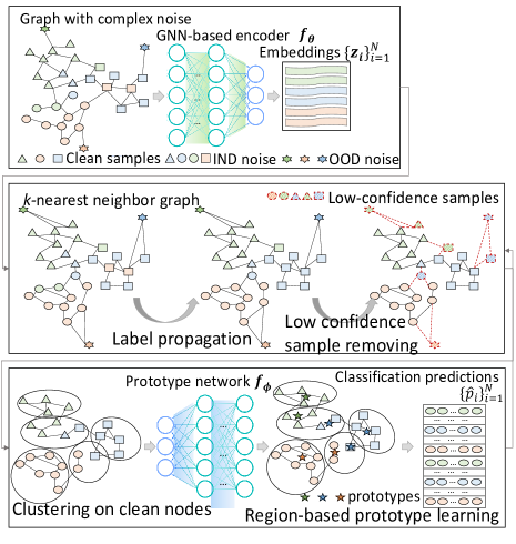
Figure 1: Overview of the proposed ROG_PL. In the latent representation space, two modules are designed: denoising via label propagation and open-set prototype learning via regions. In specific, we first correct noisy labels through similarity-based label propagation and removes low-confidence samples, to solve the intra-class variety problem caused by noise. Then we learn open-set prototypes for each known class via non-overlapped regions and remains both interior and border prototypes to remedy the inter-class confusion problem. These two modules are iteratively updated under the constraints of classification loss and prototype diversity loss.

Introduction

Graph neural networks (GNNs) (Gilmer et al. 2017; Guo et al. 2022; Hamilton, Ying, and Leskovec 2017; Tan et al. 2023) have become a prominent technique to analyze graph structured data in many real-world systems, such as traffic state prediction (Zheng et al. 2020), disease classification (Chereda et al. 2019), and user profile completion in social networks (Wong et al. 2021). The recent success of supervised GNNs is built upon two crucial cornerstones: that the training and test data are drawn from an identical distribution, and that large-scale reliable high-quality labeled data are available for training. However, in real-world applications, large-scale labeled data drawn from the same distribution as test data are usually unavailable.

Real-world applications normally are in open-set scenarios (Zhang et al. 2023a; Nimah et al. 2021; Zhang et al. 2022), the existence of new-emerged out-of-distribution (OOD) samples, i.e.samples that do not belong to any known classes, is prevalent. They are outliers if they occur in training (OOD noise), and open-set samples if they occur in testing. Moreover, the manually generating clean labeled data set would involve domain experts evaluating the quality of collected data and thus is very expensive and time-consuming (Zhang, Luo, and Gu 2023). Alternatively, we can collect data and labels based on web search (Yu et al. 2018), crowdsourcing  (Fang, Yin, and Tao 2014; Li et al. 2017a) and user tags (Li et al. 2017b; Xiao et al. 2015). These data and labels are cheap but inevitably noisy (Zhang, Luo, and Gu 2023; Li et al. 2022).

The presence of OOD noise and IND noise ( in-distribution samples with incorrect labels) can be detrimental to GNNs (Zhang et al. 2021), as they would cause the ambiguity problem, including the intra-class variety problem in which samples with same class labels may contain objects of different semantic categories, and the inter-class confusion problem in which samples of different intent classes may contain objects of similar semantic categories(Wang et al. 2023). The open-set unknown class samples occur during testing further complicates this problem.

Thus, it is necessary to build robust open-set learning models (Wu et al. 2021) that can learn from noisy data, achieving classification of known class samples and identification of unknown open-set class samples during testing. Previous works mainly concentrated on robust learning or open-set learning separately, the problem of robust open-set learning with complex noise has not been sufficiently explored so far (Huang, Wang, and Fang 2022; Zhang et al. 2023b), and it becomes even more difficult for non-IID graph data.

In this paper, as shown in Fig. 1, for solving the problem of open-set graph learning with complex IND and OOD noise, we propose a new framework ROG_PL to do robust open-set node classification. It consists of two main steps: denoising via label propagation and open-set prototype learning via regions. Specifically, in the latent representation space, ROG_PL first corrects noisy labels through similarity-based pseudo-label propagation and remove low-confidence samples, to solve the intra-class variety problem caused by noise. Then the second module learns open-set prototypes for each known class via non-overlapped regions and remains both interior and border prototypes to remedy the inter-class confusion problem. The two modules are iteratively updated under the constraints of both classification loss and prototype diversity loss. Experimental evaluations of ROG_PL on several benchmark graph datasets demonstrates that it has good performance.

Preliminaries

This study focuses on the node classification problem for a graph. A graph is denoted as $G=(V,E,X)$, where $V=\{v_{i}|{i=1,\ldots,N}\}$ is a set of $N$ nodes in the graph, and $E=\{e_{i,j}|i,j=1,\ldots,N.$ $i\neq j\}$ is a set of edges connecting pairs of nodes $v_{i}$ and $v_{j}$. $X\in\mathbb{R}^{N\times s}$ denotes the feature matrix of nodes, where $s$ is the dimension of node features. The feature vector of each node $v_{i}$ is indicated by $x_{i}\in X$. The topological structure of $G$ is represented by an adjacency matrix $A\in\mathbb{R}^{N\times N}$, where $A_{i,j}=1$ if the nodes $v_{i}$ and $v_{j}$ are connected, i.e., $\exists e_{i,j}\in E$, and otherwise $A_{i,j}=0$. The label matrix of $G$ is $Y\in\mathbb{R}^{N\times C}$, where $C$ is the already-known node classes. If a label $c$ is assigned to a node $v_{i}\in V$, then $y_{i,c}=1$, and otherwise, $y_{i,c}=0$.

For a typical closed-set node classification problem, a GNN encoder $f_{\theta_{g}}$ takes the node features $X$ and adjacency matrix $A$ as input, aggregates the neighborhood information and outputs representations. Then, a classifier $f_{\theta_{c}}$ is used to classify the nodes into $C$ already-known classes. The GNN encoder and the classifier are optimized to minimize the expected risk  (Yu et al. 2017) in Eq. (1), assuming that the testing data $\mathcal{D}_{te}$ and the training data $\mathcal{D}_{tr}$ have the same feature space and label space, i.e.,

$$f^{*}=arg\min_{f\in\mathcal{H}}\mathbb{E}_{(x,y)\sim\mathcal{D}_{te}}\mathbb{I}(y\neq f(\theta_{g},\theta_{c};x,A))$$ (1)

where $\mathcal{H}$ is the hypothesis space, $\mathbb{I}(\cdot)$ is the indicator function which outputs 1 if the expression holds and 0 otherwise. This function can be generally optimized using cross-entropy to distinguish between known classes.

In the open-set node classification problem, given a graph $G=(V,A,X)$, $\mathcal{D}_{tr}=(X,Y)$ denotes the training nodes. The test nodes are denoted by $\overline{\mathcal{D}}_{te}=(X_{te},Y_{te})$, where $X_{te}=S\cup U$, $Y_{te}=\{1,\ldots,C,C+1,\ldots\}$. The set $S$ is the nodes that belong to seen classes that already appeared in $\mathcal{D}_{tr}$ and $U$ is the set of nodes that do not belong to any seen class (i.e., unknown class nodes). The goal of open-set node classification is to learn a $(C+1)$-$class$ classifier $f_{\overline{\theta}_{c}}$ such that $f(\theta_{g},\overline{\theta}_{c};X_{te},\overline{A}):\{X_{te},\overline{A}\}\rightarrow\overline{\mathcal{Y}}$, $\overline{\mathcal{Y}}=\{1,\ldots,C,unknown\}$, by minimizing the expected risk (Yu et al. 2017):

$$\overline{f}^{*}=arg\min_{f\in\mathcal{H}}\mathbb{E}_{(x,y)\sim\mathcal{\overline{D}}_{te}}\mathbb{I}(y\neq f(\theta_{g},\overline{\theta}_{c};x,\overline{A}))$$ (2)

where $\overline{A}$ is the adjacency matrix for $X_{te}$. The predicted class $unknown\in\overline{\mathcal{Y}}$ consists of a group of novel categories, which may contain multiple classes. An intuitive way of transforming a close-set classifier into an open-set classifier is thresholding (Hendrycks and Gimpel 2017).

In the problem of Open-set node classification with IND noise and OOD noise, given a graph $G=(V,A,X)$, $\mathcal{D}_{tr}=(X,Y=S)=\{x_{i},y_{i}\}_{i=1}^{N}$ is the training set and $\mathcal{D}_{te}=(X_{te},Y_{te}=S\cup U)$ is the test set. In $\mathcal{D}_{tr}$, we assume that the instance-label pair $(x_{i},y_{i})$ , $1\leq i\leq N$, consists of three types. Let $y_{i}^{*}$ denote the ground-truth label of $x_{i}$. A clean sample is a node whose assigned label matches the ground-truth label, i.e., $y_{i}=y_{i}^{*}$. An IND noise sample is a node whose assigned label does not match the ground-truth label, but the node matches one of the classes in $S$, i.e.$y_{i}\neq y_{i}^{*},y_{i}^{*}\in S$. An OOD noise sample is a node whose assigned label does not match the ground-truth label and any known class label neither, i.e.$y_{i}\neq y_{i}^{*},y_{i}^{*}\notin S$. Moreover, under the strict setting of open-set classification, it is assumed that the ground-truth label of OOD noise $y_{i}^{*}\notin U$, i.e., there is no overlap between the classes of OOD noise and the unknown classes in the test set. Due to the memorization effect (Arpit et al. 2017), noisy data can severely impair the performance of network training. Therefore, it is desirable to develop noise-robust methods for open-set node classification, which can handle complex and diverse noises. The ultimate goal is to learn a noise-robust open-set node classifier that can minimize the expected risk in Eq. (2).

Methodology

For solving the problem of open-set graph learning with complex IND and OOD noise, we propose a new framework ROG_PL, which consists of two main steps: denoising via label propagation and open-set prototype learning via regions. As shown in Fig. 1, in the latent representation space, we first corrects noisy labels through soft pseudo-label propagation and removes low-confidence samples, to solve the intra-class variety problem caused by noise. Then we learn open-set prototypes for each known class via non-overlapped regions and remains both interior and border prototypes to remedy the inter-class confusion problem. The two modules are iteratively updated under the constraints of both classification loss and prototype diversity loss.

Denoising via Label Propagation

Inspired by label propagation algorithms for semi-supervised learning(Grandvalet and Bengio 2004; Iscen et al. 2018; Chandra and Kokkinos 2016), which seek to transfer labels from supervised examples to neighboring unsupervised examples according to their similarity in feature space, we leverage neighbour consistency to modify the supervision of each sample and to correct noise. First, we build a $k$-nearest neighbor graph $G_{N}$ upon $Z$, where $Z\in\mathbb{R}^{N\times K}$ is the latent representation given by an encoder network $f_{\theta}$ by taking the nodes feature $X$, i.e.$z_{i}=f_{\theta}(x_{i})$. $K$ indicates the dimension of the representation vectors and is determined by the network $f_{\theta}$.

In graph $G_{N}$, the affinity matrix $W\in\mathbb{R}^{N\times N}$ is encoded by the similarities between vertices, which is obtained by:

$$W_{ij}=\left\{\begin{aligned} &[z_{i}^{\top}z_{j}]_{+}^{\beta},&\text{if}~{}i\neq j\land x_{j}\in N_{k}(x_{i}),\\ &0,&\text{otherwise.}\end{aligned}\right.$$ (3)

where $N_{k}(x_{i})$ is a similarity-based neighborhood set, i.e.the set of $k$ nearest neighbors of $x_{i}$ in $X$, and $\beta$ is a parameter for diffusion on region manifolds(Chandra and Kokkinos 2016; Iscen et al. 2017)which we simply set as $\beta$ in our experiments.

Suppose we have clean nodes along with some noisy nodes, label propagation spreads the label information of each node to the other nodes based on the connectivity in the graph $G_{N}$. To weaken the influence of noisy labels, we set $\tilde{y}_{i}=y_{i}$ to the one-hot label vector of $x_{i}$ if $x_{i}$ is selected as a clean sample by Eq.(5), otherwise we use category prediction which is a $C$-dimensional vector representing the belongingness of $x_{i}$ to the $C$ known classes, i.e.$\tilde{y}_{i}=\hat{p}_{i}$, as shown in Eq. (8). The propagation process is repeated until a global equilibrium state is achieved, and each example is assigned to the class from which it has received the most information.

Formally, for graph $G_{N}=(W,X)$, $D$ is the degree matrix ( a diagonal matrix with entries $D_{ii}=\sum_{j}W_{ij}$), label propagation (Iscen et al. 2019) can be computed by minimizing

$$J(\bar{Y})=\sum_{i=1}^{N}\|\bar{y}_{i}-\tilde{y}_{i}\|+\alpha\sum_{i,j=1}^{N}W_{ij}\|\frac{1}{\sqrt{D_{ii}}}\bar{y}_{i}-\frac{1}{\sqrt{D_{jj}}}\bar{y}_{j}\|^{2}$$ (4)

where $\alpha$ is a regularization parameter to balance the fitting constraint (the first term) and the smoothing term (the second term). The fitting constraint encourages the classification of each node to their assigned label, and the smoothing term encourages the outputs of nearby points in the graph to be similar (Iscen et al. 2019). The obtained $\bar{Y}=[\bar{y}_{1},\ldots,\bar{y}_{N}]\in\mathbb{R}^{N\times C}$ is the refined soft pseudo-labels for $X$ after label propagation, further we transform $\bar{Y}$ into hard pseudo-labels by taking the largest prediction score to guide the training.

Finally, we use a sufficiently high threshold $\eta\in[0,1]$ to select a reliable subset of nodes as the clean dataset:

$$g_{i}=\left\{\begin{aligned} &1,&\text{if}~{}\bar{Y}_{iy_{i}}^{(t)}>\frac{1}{C},\\ &\mathbb{I}[\max_{c}\bar{Y}_{ic}^{(t)}>\eta],&\text{otherwise.}~{}~{}~{}~{}~{}\\ \end{aligned}\right.$$ (5)

where $\mathbb{I}(\cdot)$ is the indicator function which outputs 1 if the expression holds and 0 otherwise. $t$ denotes the number of iteration rounds. $g_{i}$ is a binary indicator representing the conservation of node $v_{i}\in V$ when $g_{i}=1$ and the removal of node $v_{i}$ when $g_{i}=0$. Thus, the clean node set $V_{cln}=\{v_{i}\|\forall v_{i}\in V\wedge g_{i}=1\}=V\backslash\{v_{i}\|\forall v_{i}\in V\wedge g_{v}=0\}$.

Open-Set Prototype Learning via Regions

Overview. With the filtered training data (clean node set $V_{cln}$), different from the conventional classification paradigm which directly feeds node features into a GNN to predict the class label, we aim at learning multiple representative prototypes for each category, and predicting class label by calculate the similarity between the node and prototypes. Upon the latent representation $Z$, in the latent representation space, we learn the prototypes. The prototype pool can be represented as $P=\{P_{1},P_{2},...,P_{C}\}$ where $C$ is the number of known classes. $P_{c}=\{p_{c,1},p_{c,2},\cdots,p_{c,K_{c}}\}\in\mathbb{R}^{K_{c}\times D}$ denotes the prototypes of category $c$ and $K_{c}$ indicates the number of prototypes of category $c$. Given a node $x_{i}$, after obtaining the high-level feature representation $z_{i}$, we compare it with all prototypes via calculating cosine similarity:

$$s_{c,k}^{(i)}=\frac{z_{i}\cdot p_{c,k}}{\|z_{i}\|\|p_{c,k}\|}$$ (6)

After obtain similarity with all prototypes,we regard the class-wise largest similarity score to obtain the scores of $x_{i}$ belonging to class $c$, i.e.,

$$s_{c}^{(i)}=\max_{k}(s_{c,1}^{(i)},\ldots,s_{c,k}^{(i)},\ldots,s_{c,K_{c}}^{(i)})$$ (7)

And the vector of score of belonging between $x_{i}$ and each class is

$$\hat{p}_{i}=[s_{1}^{(i)},s_{2}^{(i)},\ldots,s_{C}^{(i)}]$$ (8)

The final classification prediction of $x_{i}$ is

$$\hat{y}_{i}=\arg\max_{c}{\hat{p}_{i,c}}=\arg\max_{c}{s_{c}^{(i)}}$$ (9)

Open-Set Prototype Learning. The open-set node classification is different with the closed set classification problem, in which the class boundaries of known classes require to be tight and clear. Traditional prototype (Yang et al. 2018) learning normally use typical interior prototypes (such as the mean vectors of node representation in the same class) to represent the class. However, we argue that border prototypes are also crucial for classification, especially for open-set scenarios, since they provide more detailed information for preserving discrimination between classes and the information of class boundaries. We believe the combination of interior prototypes and border prototypes can well relieve the intra-class variety problem caused by the noise and inter-class confusion problem, and obtain tight and clear boundaries for known class, reserve more space for unknown classes.

Since the original training data containing IND and OOD noises, to avoid the ambiguity problem caused by noise data, we optimize the prototype learning based on the clean nodes $V_{cln}$ and the refined label annotations $\bar{Y}$. We first divide the latent space into regions by clustering the clean nodes where any clustering algorithm could be used, and we use $K$-means for its simplicity. With the obtained clusters, under the guidance of label matrix $\bar{Y}$, we use homogeneous clusters to update the interior prototypes and use non-homogeneous clusters to obtain border prototypes.

To obtain the most representative interior prototype for each class, we make interior prototypes as trainable weights of a feed forward network $f_{\phi}$ and initialized with He initialization(Liu et al. 2022). For brevity, we denote the interior prototypes by matrix

$$P_{I}=[P^{I}_{1},\ldots,P^{I}_{C}]\in\mathbb{R}^{C\times D}$$ (10)

$P^{I}_{c}$ is the interior prototype for class $c$. We update the interior prototype network $f_{\phi}$ and representation learning network $f_{\theta}$ iteratively. Since a rapidly changing of prototypes may disorganize the representativeness of the learned prototypes and make the training process unstable, we utilize a small learning rate to dynamically and smoothly update the prototypes through back-propagation:

$$P^{I}_{c,(t)}=P^{I}_{c,(t-1)}-\varphi\frac{\partial\mathcal{L}}{\partial P^{I}_{c}}$$ (11)

where $P^{I}_{c,(t)}$ and $P^{I}_{c,(t-1)}$ are the interior prototype of class $c$ at epoch $t$ and epoch $t-1$ respectively. $\mathcal{L}$ is the total loss shown as Eq. (15). $\varphi$ is the learning rate which is set as small numbers. Note that here we only use the samples in the homogeneous clusters to update the corresponding interior prototypes, i.e.we select the regions containing nodes belonging to a single class, and use these nodes to update the interior representative prototype for the corresponding class.

Towards border prototypes, the idea is to analyze those regions which contain nodes belonging to different classes. We obtain border prototypes by computing the mean vector of nodes with the same class label in non-homogeneous clusters. For example, suppose a cluster $R_{k}$ insists of samples of two classes, i.e.$M_{k}=\bar{V}_{1}^{k}\cup\bar{V}_{2}^{k}\cup\ldots\cup\bar{V}_{C}^{k}$, where $\bar{V}_{c}^{k}$ consists of a couple of nodes from class $c$, and there exists $m,n\in\{1,\ldots,C\}$ such that $\bar{V}_{m}^{k}\neq\emptyset~{}\wedge~{}\bar{V}_{n}^{k}\neq\emptyset$, then we can obtain border prototypes of class $m$ and $n$ by:

$$P_{m}^{k}=\frac{1}{\|\bar{V}_{m}^{k}\|}\sum_{v_{i}\in\bar{V}_{m}^{k}}z_{i},~{}~{}P_{n}^{k}=\frac{1}{\|\bar{V}_{n}^{k}\|}\sum_{v_{i}\in\bar{V}_{n}^{k}}z_{i}$$ (12)

It is the same for clusters that contain nodes from several different classes.

We utilize cross-entropy loss to train the encoder network $f_{\theta}$ and prototype network $f_{\phi}$ on clean nodes $V_{cln}$, under the supervision of refined class label $\bar{Y}$:

$$\mathcal{L}_{cls}=-\frac{1}{N}\sum_{i=1}^{N}\bar{y}_{i}\log\frac{exp(s_{\bar{y}_{i}}^{(i)}/T)}{\sum_{c=1}^{C}\exp{(s_{c}^{(i)}/T)}}$$ (13)

where $T$ is a temperature hyperparameter that we introduced to make the results more differentiated (Agarwala et al. 2020).

With the adoption of both interior and border prototypes, the diversity of prototypes within a class can be well mined. To further relieve the inter-class confusion problem, we hope the prototypes of different categories also away from each other. Thus, we enhance the diversity of the prototypes of known classes by adopting the orthogonal constraint to keep the orthogonality of interior prototypes by using the diversity loss:

$$\mathcal{L}_{div}=\|P_{I}P_{I}^{\top}-I\|_{F}^{2}$$ (14)

where $\|\cdot\|_{F}$ is the Frobenius-norm and $I$ is the identity matrix of any desired dimension. The overall loss function of ROG_PL is:

$$\mathcal{L}=\mathcal{L}_{cls}+\lambda\mathcal{L}_{div}$$ (15)

where $\lambda$ is the loss hyper-parameter.

So far, we obtain interior prototype and border prototypes for each known class, and we predict the class label of clean nodes through Eq. (7) and (9). To make a hard prediction, we adopt a probability threshold $\tau$, such that a testing point $x_{i}$ is deemed as an unknown class sample if $\max_{c}\hat{p}_{i,c}<\tau$.

Experiments

We design our experiments to evaluate ROG_PL, focusing on the following aspects: open-set classification comparison, robustness analysis, and ablation study. Codes will be available online.

Experimental Setup

Dataset and Metrics. To evaluate the performance of the proposed framework for robust open-set node classification, We conducted experiments on three main benchmark graph datasets (Wu, Pan, and Zhu 2020; Zhu et al. 2022), namely Cora, Citeseer (Yang, Cohen, and Salakhudinov 2016), and Coauthor-CS (Zhou et al. 2023), which are widely used citation network datasets. The statistics of the datasets are presented in the Appendix. In terms of the metrics, following the study of Wu et al. (Wu et al. 2021), we adopt macro-F1 and AUROC to measure the performance.

Implementation Details. In the experiments, we adopt GCN (Kipf and Welling 2016) as backbone neural network for the encoder $f_{\theta}$, configured with two hidden layers with a dimension of 128. The prototype network $f_{\phi}$ configured with a linear layer with a dimension of $C+1$. ROG_PL is implemented with PyTorch and the networks are optimized using adaptive moment estimation with a learning rate of $10^{-3}$. The balance parameters $\lambda$ is set to $10^{-2}$. The threshold $\eta$ were selected by a grid search in the range from $0$ to $1$ with a step of $10^{-1}$. The number of nearest neighbors $k$ were selected by a grid search in the range from $30$ to $35$ with a step of $1$.

For each experiment, the baselines and the proposed method were applied on the same training, validation, and testing datasets. All the experiments were conducted on a workstation equipped with an Intel(R) Xeon(R) Gold 6226R CPU and an Nvidia A100 GPU.

Test Settings. To evaluate the performance of open-set node classification, for each dataset, the data of several classes were held out as the unknown classes for testing and the remaining classes were considered as the known classes. 70% of the known class nodes were sampled for training, 10% for validation, and 20% for testing.

To assess the performance of the proposed ROG_PL framework on graph data with different noises, we tested it with mixed IND and OOD noise. In the training set, we randomly selected 5%/25%/50% of the known class samples to be IND noise, and randomly replaced their ground-truth labels with wrong known class labels. Then, we used the nodes from neither the known classes of the training set nor the unknown classes of the test set as OOD noise, and randomly assigned known class labels to them. The samples with right known class labels (clean data), the known class samples with incorrect labels (IND noise) and the far-away unknown class samples with wrong known class labels (OOD noise) constitute the final training set. The test set includes the known class samples and the unknown class samples, where the unknown classes are different from the classes of OOD noise. The setting of inductive learning was adopted for all the experiments, where no information about the unknown class in the test set (such as the feature $x_{i}$ or other side information of unknown classes) is utilized during training or evaluation.

Methods			GCN_soft	GCN_sig	GCN_soft$\_\tau$	GCN_sig$\_\tau$	NWR_$\tau$	Openmax	OpenWGL	$\mathcal{G}^{2}Pxy$	NGC	PNP	ROGPL
Cora	5%	F1	63.73	64.12	70.53	57.80	69.41	60.40	73.03	72.00	59.69	70.26	78.36
		AUROC	fail	fail	82.82	81.40	75.05	67.26	79.36	78.30	78.20	82.04	91.00
	25%	F1	64.31	63.78	70.69	66.91	68.98	59.82	70.58	69.92	52.13	64.78	77.59
		AUROC	fail	fail	77.92	79.94	81.69	87.61	77.90	77.36	80.22	84.87	91.59
	50%	F1	60.96	59.73	62.53	62.93	61.93	53.50	63.59	57.52	62.70	66.29	76.90
		AUROC	fail	fail	79.46	78.52	78.73	80.88	85.40	63.68	83.64	83.54	90.47
Citeseer	5%	F1	39.03	37.74	59.13	59.93	52.28	33.23	59.87	52.40	59.44	59.99	62.24
		AUROC	fail	fail	85.67	85.56	76.13	55.01	86.08	67.75	84.05	85.70	87.84
	25%	F1	38.30	38.02	23.04	57.79	48.51	36.70	57.42	53.53	55.42	59.83	63.89
		AUROC	fail	fail	84.50	82.26	72.59	75.68	82.34	53.97	80.46	84.03	88.84
	50%	F1	30.39	31.71	35.41	35.54	35.65	24.83	40.46	41.92	56.39	51.81	57.08
		AUROC	fail	fail	64.20	50.74	61.22	67.89	79.54	38.03	77.43	80.40	85.64
Coauthor-CS	5%	F1	75.44	76.50	76.63	71.70	75.43	62.68	74.09	83.45	77.61	83.56	81.68
		AUROC	fail	fail	83.14	86.61	89.57	81.65	87.39	82.95	85.57	85.55	93.25
	25%	F1	74.58	75.19	81.92	73.38	65.64	66.38	72.98	67.21	69.18	79.37	83.32
		AUROC	fail	fail	87.77	88.35	88.69	80.62	86.35	86.03	85.11	85.47	94.06
	50%	F1	72.93	60.77	68.87	52.63	78.66	59.97	54.70	72.96	63.06	68.40	79.29
		AUROC	fail	fail	75.02	83.97	87.58	81.48	85.13	72.87	84.27	84.85	93.31

Table 1: Comparison of open-set node classification in test F1-score and AUROC (%) on three datasets, where IND noise (5%/ 25%/ 50%) and near OOD noise is injected into training set.

Baselines. We compare ROG_PL with 10 baselines, which are from three categories.

• 1) Closed-set classification methods: GCN_soft and GCN_sig. They are GCNs (Kipf and Welling 2016) with a softmax layer or a multiple 1-vs-rest of sigmoids layer as output layer.

• 2) Open-set classification methods: GCN_soft_$\tau$, GCN_sig_$\tau$, NWR_$\tau$ (Tang, Yang, and Li 2022), Openmax (Bendale and Boult 2016), OpenWGL (Wu, Pan, and Zhu 2020) and $\mathcal{G}^{2}Pxy$ (Zhang et al. 2023b). Specifically, GCN_soft_$\tau$, GCN_sig_$\tau$ and NWR_$\tau$ are GCN_soft, GCN_sig and the original NWR (Tang, Yang, and Li 2022) methods by added a threshold chosen from $\{0.1,0.2,\ldots,0.9\}$ to perform open-set recognition. Openmax (Bendale and Boult 2016) is an open-set recognition model based on “activation vectors” (i.e. penultimate layer of the network). OpenWGL (Wu, Pan, and Zhu 2020) and $\mathcal{G}^{2}Pxy$ (Zhang et al. 2023b) are two open-set node classification methods for graph data, which has no robust learning ability.

• 3) Robust open-set classification methods: NGC (Wu et al. 2021) and PNP (Sun et al. 2022). NGC (Wu et al. 2021) is an open-world noisy data learning method for image classification which employs geometric structure and model predictive confidence to collect clean sample. PNP_$\tau$ (Sun et al. 2022) is a robust classifier learning method for image data with IND and OOD noise, where data augmentation is used to help the identification of noisy samples. To perform open-set recognition, we adopt a threshold chosen from $\{0.1,0.2,\ldots,0.9\}$ to PNP.

Note that the graph data are first embedded by a GCN before being feed into the models that cannot handle graph data. A detailed introduction can be found in the Appendix.

Open-Set Node Classification with Complex Noisy Graph Data

Considering that real-world scenarios are complex and noisy data vary across different tasks, we assessed the proposed model for open-set classification with IND noise and two types of OOD data: near OOD data and far OOD data. Here, OOD data include OOD noise in the training set and out-of-distribution samples of unknown classes that occur during testing.

Open-Set Classification with IND Noise and Near OOD Data.

In this experiment, for each dataset, following the setting of OpenWGL (Wu, Pan, and Zhu 2020), the data of the last class were held out as the unknown class for testing, and the data of the second last class which were re-assigned with random known class labels were set as the OOD noise data and injected into the training set. The remaining classes were considered as known classes, while the known class samples in training set were re-assigned with wrong known class labels with a rate of 5%, 25% and 50% (i.e.IND noise rate), respectively.

Table 1 lists the macro-F1 and AUROC scores for open-set node classification with near OOD noise and different proportions of IND noise. It is observed that ROG_PL generally obtain the best performance on the benchmarks. This shows that ROG_PL can better distinguish between a known class and an unknown class, even though there is a large amount of complex and diverse noises during training. Specifically, ROG_PL achieves an average of 6.23% improvement over the second-best method (PNP) in terms of F1 score and an average of 6.62% improvement in terms of AUROC on the three datasets.

Furthermore, we examined the detailed classification accuracy in terms of known classes and unknown classes. We found that to gain the ability of unknown class detection, compared to the closed-set classifier, there is a slight decrease in the performance of known class classification, i.e., from 86.33% (GCN_soft) to 75.48% (ROG_PL) on average, while the unknown class detection accuracy is increased from 0% to a remarkable 83.78% on average. Moreover, compared to other open-set node classification methods, such as $\mathcal{G}^{2}Pxy$, ROG_PL achieves an average improvement of 11.9%, 13.29% and 9.94% in accuracy of known classification, unknown detection and overall classification, respectively. The average improvement in F1 score is 9.94%. Details are provided in the Appendix.

Methods	5% far OOD noise						25% far OOD noise
	Cora		Citeseer		Coauthor-CS		Cora		Citeseer		Coauthor-CS
	F1	AUROC	F1	AUROC	F1	AUROC	F1	AUROC	F1	AUROC	F1	AUROC
GCN_soft	64.67	fail	39.04	fail	60.36	fail	63.12	fail	39.04	fail	77.08	fail
GCN_sig	64.11	fail	41.33	fail	69.32	fail	63.44	fail	40.78	fail	65.94	fail
GCN_soft$\_\tau$	71.81	74.61	58.57	82.35	65.81	78.37	70.38	75.13	56.09	81.61	60.48	72.37
GCN_sig$\_\tau$	62.65	77.54	54.60	84.58	54.23	86.73	69.23	76.38	57.41	81.81	57.75	84.31
NWR_$\tau$	71.94	76.58	48.35	75.06	79.46	87.65	68.79	80.67	48.08	71.67	54.77	83.76
Openmax	28.37	79.06	26.64	81.17	66.90	82.10	31.41	84.40	15.55	79.03	67.23	85.07
OpenWGL	71.83	76.76	58.51	84.78	76.38	87.24	67.87	74.50	57.28	82.75	75.71	85.10
$\mathcal{G}^{2}Pxy$	69.24	80.67	43.26	62.53	66.98	69.57	66.54	75.26	41.67	60.95	70.45	68.34
NGC	57.58	78.57	52.30	78.07	66.96	84.47	59.86	76.88	55.41	81.22	64.84	83.96
PNP	72.21	79.51	60.22	83.93	77.50	87.42	72.19	77.47	57.58	81.94	81.34	84.23
ROGPL	77.62	87.89	60.90	84.50	83.11	92.34	76.31	86.48	58.08	85.49	82.06	89.78

Table 2: Comparison of open-set node classification in test F1-score and AUROC (%) on three datasets, where IND noise (5%) and far OOD noise (5% / 25%) from the Pubmed dataset is injected into the training set.

Open-Set Node Classification with IND Noise and Far OOD Data.

To investigate the effect of rough OOD noise, we used OOD samples that are from different dataset as the source of OOD noise. Specifically, we randomly selected samples of the first two classes from Pubmed (Hu et al. 2020) and mixed them with data from Cora, Citeseer and Coauthor-CS to create the training set with far OOD noise, where the OOD noise rate is set to 5% or 25%. Each node from Pubmed was randomly assigned to a known class label, and edges between the node and its $k$-nearest neighbors were added, where $k$ is a random integer in the range from 1 to 5. We also added some samples from the remaining categories in the Pubmed dataset to the test set in corresponding proportion, to evaluate the performance of ROG_PL on the samples from far open-set. The other settings are the same as the experiment of near OOD data, and the IND noise rate is set as 5%.

The results of open-set node classification with far OOD noise are presented in Table 2. The results show that ROG_PL generally outperforms the baselines, achieving an average improved of 2.84% in F1 and an average improvement of 5.33% in AUROC, compared to the global second-best method PNP. The detailed classification accuracy in terms of known classes and unknown classes with far OOD noise are given in the Appendix.

Robustness Analysis under Different Noise Rate

In this section, we evaluate the robustness of ROG_PL for different levels of IND and OOD noise for the open-set node classification task. We first examine how ROG_PL reacts to different IND noise rate. We kept the OOD noise rate constant and used the same setting as the experiment of Table 1, while we varied the IND noise rate from 0%, 5%, 25%, 50% to 75%. Fig. 2(a) and Fig. 2(b) show the results on the Cora and Citeseer datasets, respectively. We observe that ROG_PL maintains a relatively stable performance when the noise rate is within a certain range, for example no more than 50%. However, once the IND noise exceeds a certain threshold, ROG_PL’s performance drops sharply.

Additionally, we investigate the performance of ROG_PL in terms of different OOD noise rate, by keeping the IND noise rate constant as 5%, while varying the far OOD noise rate from 0%, 5%, 25%, 50% to 75% . The results on Cora and Citeseer are shown in Fig.2(c) and Fig. 2(d)respectively. It can be observed that ROG_PL maintains a surprisingly stable performance even with large amounts of far OOD noise in the training data, which demonstrates the strong robustness of ROG_PL against OOD noise.

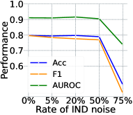
(a) Cora

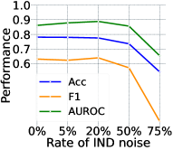
(b) Citeseer

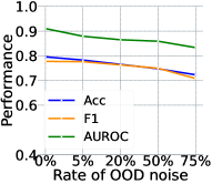
(c) Cora

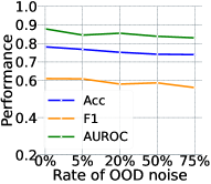
(d) Citeseer

Figure 2: The performance of ROG_PL with respect to different IND noise rate and OOD noise rate on Cora and Citeseer datasets.

Methods	Cora		Citeseer		Coauthor-CS
	F1	AUROC	F1	AUROC	F1	AUROC
ROG${}_{PL}\neg G_{N}$	74.87	89.90	61.79	86.94	81.08	91.10
ROG${}_{PL}\neg$denoise	77.24	86.56	61.24	86.99	81.03	87.86
ROG${}_{PL}\neg\mathcal{L}_{div}$	73.67	89.85	60.35	86.73	79.88	90.32
ROG${}_{PL}\neg$region	76.54	84.11	61.63	87.49	80.89	86.45
ROGPL	78.36	91.00	62.24	87.84	81.68	93.25

Table 3: Ablation study of robust open-set node classification in test F1 score and AUROC (%) on three datasets, where IND noise (5%) and near OOD noise is injected into the training set.

Ablation Study

We compare variants of ROG_PL in an ablation study to evaluate the effect of its main modules and settings:

• ROG${}_{PL}\neg G_{N}$: a variant of ROG_PL without building $k$-nearest neighbor graph $G_{N}$, and original graph $G$ is used in the label propagation stage.

• ROG${}_{PL}\neg$denoise: a variant of ROG_PL without the label propagation based denoising module.

• ROG${}_{PL}\neg$region: a variant of ROG_PL without clustering, i.e.the interior prototype of each class is updated by the clean nodes from all classes, and there is no border prototypes.

• ROG${}_{PL}\neg\mathcal{L}_{div}$: a variant of ROG_PL with loss $\mathcal{L}_{div}$ removed. We only utilize classification loss $\mathcal{L}_{cls}$ to train the encoder network $f_{\theta}$ and prototype network $f_{\phi}$.

The performance of the proposed method and its four variants are presented in Table 3. The results demonstrate that both label propagation based denoising module and region-based prototype learning module are important and building $k$nn graph $G_{N}$ is necessary. The large gap of performance between ROG_PL and ROG${}_{PL}\neg$region verifies the contribution of open-set prototypes on open-set node classification.

Conclusion

This paper introduced a novel prototype learning based robust open-set node classification method to learn an open-set classifier from graphs with mixed IND and OOD noisy nodes. By correcting noisy labels through similarity-based label propagation and removing low-confidence samples, the proposed method relieve the intra-class variety caused by noise. Further, by learning open-set prototypes via non-overlapped regions and remaining both interior and border prototypes, the method can remedy the inter-class confusion problem, and save more space for open-set classes. To the best of our knowledge, the proposed ROG_PL is the first robust open-set node classification method for graph data with complex noise. Experimental evaluations on several benchmark graph datasets demonstrates its good performance.

References

- Agarwala et al. (2020) Agarwala, A.; Pennington, J.; Dauphin, Y.; and Schoenholz, S. 2020. Temperature check: theory and practice for training models with softmax-cross-entropy losses. arXiv:2010.07344.
- Arpit et al. (2017) Arpit, D.; Jastrzebski, S.; Ballas, N.; Krueger, D.; Bengio, E.; Kanwal, M. S.; Maharaj, T.; Fischer, A.; Courville, A.; Bengio, Y.; et al. 2017. A closer look at memorization in deep networks. In International conference on machine learning, 233–242. PMLR.
- Bendale and Boult (2016) Bendale, A.; and Boult, T. E. 2016. Towards open set deep networks. In IEEE conference on computer vision and pattern recognition, 1563–1572.
- Chandra and Kokkinos (2016) Chandra, S.; and Kokkinos, I. 2016. Fast, exact and multi-scale inference for semantic image segmentation with deep gaussian crfs. In Computer Vision–ECCV 2016: 14th European Conference, Amsterdam, The Netherlands, October 11–14, 2016, Proceedings, Part VII 14, 402–418. Springer.
- Chereda et al. (2019) Chereda, H.; Bleckmann, A.; Kramer, F.; Leha, A.; and Beissbarth, T. 2019. Utilizing Molecular Network Information via Graph Convolutional Neural Networks to Predict Metastatic Event in Breast Cancer. In GMDS, 181–186.
- Fang, Yin, and Tao (2014) Fang, M.; Yin, J.; and Tao, D. 2014. Active learning for crowdsourcing using knowledge transfer. In Proceedings of the AAAI Conference on Artificial Intelligence, 1809–1815.
- Gilmer et al. (2017) Gilmer, J.; Schoenholz, S. S.; Riley, P. F.; Vinyals, O.; and Dahl, G. E. 2017. Neural message passing for quantum chemistry. In International conference on machine learning, 1263–1272. PMLR.
- Grandvalet and Bengio (2004) Grandvalet, Y.; and Bengio, Y. 2004. Semi-supervised learning by entropy minimization. Advances in neural information processing systems, 17.
- Guo et al. (2022) Guo, K.; Zhou, K.; Hu, X.; Li, Y.; Chang, Y.; and Wang, X. 2022. Orthogonal graph neural networks. In Proceedings of the AAAI Conference on Artificial Intelligence, 3996–4004.
- Hamilton, Ying, and Leskovec (2017) Hamilton, W.; Ying, Z.; and Leskovec, J. 2017. Inductive representation learning on large graphs. Advances in neural information processing systems, 30.
- Hendrycks and Gimpel (2017) Hendrycks, D.; and Gimpel, K. 2017. A baseline for detecting misclassified and out-of-distribution examples in neural networks. International Conference on Learning Representations.
- Hu et al. (2020) Hu, W.; Fey, M.; Zitnik, M.; Dong, Y.; Ren, H.; Liu, B.; Catasta, M.; and Leskovec, J. 2020. Open graph benchmark: Datasets for machine learning on graphs. Advances in neural information processing systems, 33: 22118–22133.
- Huang, Wang, and Fang (2022) Huang, T.; Wang, D.; and Fang, Y. 2022. End-to-end open-set semi-supervised node classification with out-of-distribution detection. In IJCAI, 2087–2093.
- Iscen et al. (2018) Iscen, A.; Tolias, G.; Avrithis, Y.; and Chum, O. 2018. Mining on manifolds: Metric learning without labels. In Proceedings of the IEEE Conference on Computer Vision and Pattern Recognition, 7642–7651.
- Iscen et al. (2019) Iscen, A.; Tolias, G.; Avrithis, Y.; and Chum, O. 2019. Label propagation for deep semi-supervised learning. In Proceedings of the IEEE/CVF conference on computer vision and pattern recognition, 5070–5079.
- Iscen et al. (2017) Iscen, A.; Tolias, G.; Avrithis, Y.; Furon, T.; and Chum, O. 2017. Efficient diffusion on region manifolds: Recovering small objects with compact cnn representations. In Proceedings of the IEEE conference on computer vision and pattern recognition, 2077–2086.
- Kipf and Welling (2016) Kipf, T. N.; and Welling, M. 2016. Semi-supervised classification with graph convolutional networks. arXiv:1609.02907.
- Li et al. (2022) Li, S.; Xia, X.; Ge, S.; and Liu, T. 2022. Selective-supervised contrastive learning with noisy labels. In Proceedings of the IEEE/CVF Conference on Computer Vision and Pattern Recognition, 316–325.
- Li et al. (2017a) Li, W.; Wang, L.; Li, W.; Agustsson, E.; and Van Gool, L. 2017a. Webvision database: Visual learning and understanding from web data. arXiv:1708.02862.
- Li et al. (2017b) Li, Y.; Yang, J.; Song, Y.; Cao, L.; Luo, J.; and Li, L.-J. 2017b. Learning from noisy labels with distillation. In Proceedings of the IEEE international conference on computer vision, 1910–1918.
- Liu et al. (2022) Liu, Y.; Jin, M.; Pan, S.; Zhou, C.; Zheng, Y.; Xia, F.; and Philip, S. Y. 2022. Graph self-supervised learning: A survey. IEEE Transactions on Knowledge and Data Engineering, 35(6): 5879–5900.
- Nimah et al. (2021) Nimah, I.; Fang, M.; Menkovski, V.; and Pechenizkiy, M. 2021. ProtoInfoMax: Prototypical Networks with Mutual Information Maximization for Out-of-Domain Detection. In Moens, M.-F.; Huang, X.; Specia, L.; and Yih, S. W.-t., eds., Findings of the Association for Computational Linguistics: EMNLP 2021, 1606–1617. Punta Cana, Dominican Republic: Association for Computational Linguistics.
- Sun et al. (2022) Sun, Z.; Shen, F.; Huang, D.; Wang, Q.; Shu, X.; Yao, Y.; and Tang, J. 2022. Pnp: Robust learning from noisy labels by probabilistic noise prediction. In Proceedings of the IEEE/CVF Conference on Computer Vision and Pattern Recognition, 5311–5320.
- Tan et al. (2023) Tan, R.; Tan, Q.; Zhang, Q.; Zhang, P.; Xie, Y.; and Li, Z. 2023. Ethereum fraud behavior detection based on graph neural networks. Computing, 1–28.
- Tang, Yang, and Li (2022) Tang, M.; Yang, C.; and Li, P. 2022. Graph auto-encoder via neighborhood wasserstein reconstruction. arXiv:2202.09025.
- Wang et al. (2023) Wang, B.; Yang, K.; Zhao, Y.; Long, T.; and Li, X. 2023. Prototype-based intent perception. IEEE Transactions on Multimedia.
- Wong et al. (2021) Wong, R. Y. M.; Cheung, C. M.; Xiao, B.; and Thatcher, J. B. 2021. Standing up or standing by: Understanding bystanders’ proactive reporting responses to social media harassment. Information Systems Research, 32(2): 561–581.
- Wu, Pan, and Zhu (2020) Wu, M.; Pan, S.; and Zhu, X. 2020. Openwgl: Open-world graph learning. In IEEE international conference on data mining, 681–690.
- Wu et al. (2021) Wu, Z.-F.; Wei, T.; Jiang, J.; Mao, C.; Tang, M.; and Li, Y.-F. 2021. NGC: A unified framework for learning with open-world noisy data. In Proceedings of the IEEE/CVF International Conference on Computer Vision, 62–71.
- Xiao et al. (2015) Xiao, T.; Xia, T.; Yang, Y.; Huang, C.; and Wang, X. 2015. Learning from massive noisy labeled data for image classification. In Proceedings of the IEEE conference on computer vision and pattern recognition, 2691–2699.
- Yang et al. (2018) Yang, H.-M.; Zhang, X.-Y.; Yin, F.; and Liu, C.-L. 2018. Robust classification with convolutional prototype learning. In Proceedings of the IEEE conference on computer vision and pattern recognition, 3474–3482.
- Yang, Cohen, and Salakhudinov (2016) Yang, Z.; Cohen, W.; and Salakhudinov, R. 2016. Revisiting semi-supervised learning with graph embeddings. In International conference on machine learning, 40–48. PMLR.
- Yu et al. (2018) Yu, X.; Liu, T.; Gong, M.; and Tao, D. 2018. Learning with biased complementary labels. In Proceedings of the European conference on computer vision (ECCV), 68–83.
- Yu et al. (2017) Yu, Y.; Qu, W.-Y.; Li, N.; and Guo, Z. 2017. Open-category classification by adversarial sample generation. In International Joint Conference on Artificial Intelligence, 3357–3363.
- Zhang et al. (2021) Zhang, C.; Bengio, S.; Hardt, M.; Recht, B.; and Vinyals, O. 2021. Understanding deep learning (still) requires rethinking generalization. Communications of the ACM, 64(3): 107–115.
- Zhang, Luo, and Gu (2023) Zhang, C.; Luo, L.; and Gu, B. 2023. Denoising Multi-Similarity Formulation: A Self-Paced Curriculum-Driven Approach for Robust Metric Learning. In Proceedings of the AAAI Conference on Artificial Intelligence, 11183–11191.
- Zhang et al. (2023a) Zhang, Q.; Chen, S.; Xu, D.; Cao, Q.; Chen, X.; Cohn, T.; and Fang, M. 2023a. A Survey for Efficient Open Domain Question Answering. In Rogers, A.; Boyd-Graber, J.; and Okazaki, N., eds., Proceedings of the 61st Annual Meeting of the Association for Computational Linguistics (Volume 1: Long Papers), 14447–14465. Toronto, Canada: Association for Computational Linguistics.
- Zhang et al. (2022) Zhang, Q.; Li, Q.; Chen, X.; Zhang, P.; Pan, S.; Fournier-Viger, P.; and Huang, J. Z. 2022. A Dynamic Variational Framework for Open-World Node Classification in Structured Sequences. In 2022 IEEE International Conference on Data Mining (ICDM), 703–712. IEEE.
- Zhang et al. (2023b) Zhang, Q.; Shi, Z.; Zhang, X.; Chen, X.; Fournier-Viger, P.; and Pan, S. 2023b. G2Pxy: generative open-set node classification on graphs with proxy unknowns. In Proceedings of the Thirty-Second International Joint Conference on Artificial Intelligence, 4576–4583.
- Zheng et al. (2020) Zheng, C.; Fan, X.; Wang, C.; and Qi, J. 2020. Gman: A graph multi-attention network for traffic prediction. In AAAI Conference on Artificial Intelligence, 1234–1241.
- Zhou et al. (2023) Zhou, B.; Jiang, Y.; Wang, Y.; Liang, J.; Gao, J.; Pan, S.; and Zhang, X. 2023. Robust graph representation learning for local corruption recovery. In Proceedings of the ACM Web Conference 2023, 438–448.
- Zhu et al. (2022) Zhu, Q.; Zhang, C.; Park, C.; Yang, C.; and Han, J. 2022. Shift-Robust Node Classification via Graph Adversarial Clustering. arXiv:2203.15802.