Supersymmetric AdS Solitons and the interconnection of different vacua of ${\cal N}=4$ Super Yang-Mills

Andrés Anabalón${}^{\leavevmode\nobreak\ a\leavevmode\nobreak\ b}$, Horatiu Nastase${}^{\leavevmode\nobreak\ b}$ and Marcelo Oyarzo${}^{\leavevmode\nobreak\ a}$

^(a)Departamento de Física, Universidad de Concepción, Casilla, 160-C, Concepción, Chile.
^(b)Instituto de Física Teórica, UNESP-Universidade Estadual Paulista
Rua Dr. Bento T. Ferraz 271, Bl. II, Sao Paulo 01140-070, SP, Brazil.

We find AdS soliton solutions in 5-dimensional gauged supergravity, obtained from the $S^{5}$ compactification of type IIB, with a dilaton saturating the Breitenlohner-Freedman bound. The solutions depend on the value of the periodicity of an $S^{1}$ cycle and the boundary values for two $U(1)$ gauge fields, and give a scalar VEV in the dual field theory. At certain values of the gauge sources we have supersymmetric solutions, corresponding to supersymmetric flows, which are a deformation of the Coulomb Branch flow in ${\cal N}=4$ SYM. The solutions parameterize quantum phase transitions between a discrete spectrum phase, a continuous above a mass gap phase, and a continuous without a mass gap phase, in 2+1 dimensions. We analyze the phase diagram in terms of the QFT sources and we find that for every value for them, there are always two branches of supergravity solutions. We find that these two branches of solitons correspond to two possible vacua existing in the dual QFT when fermions are anti-periodic on an $S^{1}$. We describe the interconnection of these states in the QFT at strong ’t Hooft coupling in the large $N$ limit. In 10 dimensions, our solutions are related to deformations of D3-brane distributions.

1 Introduction

In the AdS/CFT correspondence, the Witten model [1], corresponding to a scaling $M\rightarrow\infty$ of a Schwarzschild-AdS black hole, or to a near-horizon near-extremal limit of D3-branes, is interpreted as dual to ${\cal N}=4$ SYM at finite temperature or, after a double Wick rotation by replacing the periodic time $t$ with a Kaluza-Klein (KK) angular coordinate $\phi$, and a reduction on $\phi$, as dual to 3-dimensional pure glue theory ($\equiv QCD_{3}$; fermions are antiperiodic, so massive and scalars gain a mass at one-loop, from the fermions), coupled to extra modes at the KK scale $T_{\rm KK}=1/R_{\phi}$, and one obtains a discrete spectrum of states. This is also similar to what one obtains by cutting off AdS space in the IR (the “hard-wall” model).

But there are other behaviours possible from deforming ${\cal N}=4$ SYM. One such is the “Coulomb Branch (CB)” deformation of ${\cal N}=4$ SYM, by a scalar operator of dimension $\Delta=2$, studied in [2]. One obtains two possible metrics, described by dimensionless parameters $\pm\ell^{2}/L^{2}$, describing either discrete states (for minus sign) or continuous above a mass gap (for plus sign).

In another development, in asymptotically flat spacetime, the boundary conditions associated with the KK soliton [3], a double Wick rotation of the Schwarzschild black hole, makes the KK vacuum with antiperiodic boundary conditions for the fermions unstable towards decay, as the gravitational Hamiltonian is unbounded from below in this case. However, the AdS soliton [4], which also has antiperiodic conditions for the fermions on an $S^{1}$, is perturbatively stable, though susy- breaking. Recently it was shown that supersymmetric AdS solitons exist [5, 6, 7], and the charged solitons (for the AdS Einstein-Maxwell theory) generate phase transitions in the dual field theory. These ideas have also been generalized to 10 dimensions, representing new models of holographic confinement [8, 9, 10, 11].

In this paper, we will find AdS soliton-like solutions in the well known STU model of type IIB supergravity. In general its field content is that of 3 $U(1)$ gauge fields and 2 scalars. It is a consistent truncation of the 5-dimensional maximal gauged supergravity that one gets from type IIB supergravity compactified on an $S^{5}$. As such, this solution should describe a deformation of ${\cal N}=4$ SYM, and we will find that there is a deformation of the Coulomb branch solution of [2], that interpolates between various possibilities for the spectrum, thus generating phase transitions in the field theory in 2+1 dimensions. For every possible value of the boundary sources, there are two possible AdS soliton like solutions [5]. In the field theory, we find that there are two possible vacua in $\mathcal{N}=4$ Super Yang-Mills when the fermions are anti-periodic on an $S^{1}$. Thus, the solitons nicely describe this degeneracy and holography yields the strongly coupled phase diagram of $\mathcal{N}=4$ Super Yang-Mills in the large $N$ limit.

The paper is organized as follows. In section 2 we describe the model and the supersymmetric solutions. In section 3 we describe the general solutions, have a first go at a field theory interpretation, and the parametrization of the space of solutions. In section 4 we describe holographic renormalization and describe the phase diagram from the point of view of gravity. Then we show that when the fermions are anti-periodic on the $S^{1}$, one can have two possible states in the dual $\mathcal{N}=4$ Super Yang-Mills, and we match these two results. In section 5 we uplift the solution to 10 dimensions, describe the result in terms of deformations of distributions of D3-branes, and analyze the mass spectra in order to obtain a field theory interpretation of the phase transitions. In section 6 we conclude, and the appendices give details on solving a relevant equation and the integrability conditions for the supersymmetry transformations. We also have an appendix on a possible interpretation of the solutions in terms of the Wick rotation of rotating D3-branes in 10 dimensions.

2 The model

We are interested in studying a truncation of type IIB supergravity compactified over the $S^{5}$ with action

$$S_{0}=\frac{1}{2\kappa}\int\sqrt{-g}\left(R-\frac{\left(\partial\Phi_{1}\right)^{2}}{2}-\frac{\left(\partial\Phi_{2}\right)^{2}}{2}+\sum_{i=1}^{3}4L^{-2}X_{i}^{-1}-\frac{1}{4}X_{i}^{-2}(F^{i})^{2}+\frac{1}{4}\epsilon^{\mu\nu\rho\sigma\lambda}A^{1}_{\mu}F^{2}_{\nu\rho}F^{3}_{\sigma\lambda}\right)d^{5}x,$$ (2.1)

where $F^{i}$ are two forms, related with gauge fields in the standard way, $F_{i}=d\bar{A}_{i}$, $X_{i}=e^{-\frac{1}{2}\vec{a}_{i}\cdot\vec{\Phi}}$, $\vec{\Phi}=\left(\Phi_{1},\Phi_{2}\right)$ and

$$\vec{a}_{1}=\left(\frac{2}{\sqrt{6}},\sqrt{2}\right),\qquad\vec{a}_{2}=\left(\frac{2}{\sqrt{6}},-\sqrt{2}\right),\qquad\vec{a}_{3}=\left(-\frac{4}{\sqrt{6}},0\right).$$ (2.2)

We remark that we have changed the standard coupling constant of the gauged supergravity by the AdS radius $L$ through the relation $g=\frac{1}{L}$. We will be interested in purely magnetic solutions, in which case it is consistent to truncate the axions to zero. The Lagrangian (2.1) can be obtained from the compactification of ten dimensional type IIB supergravity over the five sphere with the ansatz [12]

$$ds_{10}^{2} =\tilde{\Delta}^{1/2}ds_{5}^{2}+L^{2}\tilde{\Delta}^{-1/2}\sum_{i=1}^{3}X_{i}^{-1}\left(d\mu_{i}^{2}+\mu_{i}^{2}\left(d\phi_{i}+\frac{1}{L}A_{i}\right)^{2}\right),$$ (2.3)

$$F_{5} =G_{5}+*G_{5},$$ (2.4)

$$G_{5} =\frac{2}{L}\epsilon_{5}\sum_{i=1}^{3}\left(X_{i}^{2}\mu_{i}^{2}-\tilde{\Delta}X_{i}\right)-\frac{L}{2}X_{i}^{-1}\ast_{5}dX_{i}\wedge d\mu_{i}^{2}$$ (2.5)

$$+L^{2}\sum_{i}X_{i}^{-2}\mu_{i}d\mu_{i}\wedge\left(d\phi_{i}+\frac{1}{L}A_{i}\right)\wedge\ast_{5}F_{i},$$ (2.6)

where $*$ is the Hodge dual with respect to the ten-dimensional metric, $\ast_{5}$ is the Hodge dual with respect to the five-dimensional metric $ds_{5}^{2}$, $\epsilon_{5}$ is its volume form, and $F_{5}$ is the self-dual five-form field strength of type IIB supergravity. The $\phi_{i}$ are $2\pi$ periodic angular coordinates parametrizing the three independent rotations on $S^{5}$, $\tilde{\Delta}=\sum_{i}X^{i}\mu^{2}_{i}$ and $\sum_{i}\mu^{2}_{i}=1$. We will be interested in considering the higher-dimensional interpretation of some of our solutions using this uplift.

The equations of ten-dimensional IIB supergravity in the metric-dilaton-$F_{5}$ sector are given by

$$R_{\mu\nu}+2\nabla_{\mu}\nabla_{\nu}\phi_{D}-\frac{e^{2\phi_{D}}}{4}\left(\frac{1}{4!}F_{\mu\rho_{1}\dots\rho_{4}}F_{\nu}^{\ \rho_{1}\dots\rho_{4}}-\frac{1}{2}g_{\mu\nu}\frac{1}{5!}F_{\rho_{1}\dots\rho_{5}}F^{\rho_{1}\dots\rho_{5}}\right) = 0\ .$$ (2.7)

$$R-4\left(\partial\phi_{D}\right)^{2}+4e^{-2\phi_{D}}\square\phi_{D} = 0\ ,$$ (2.8)

$$dF_{5} = 0\ ,$$ (2.9)

where $\phi_{D}$ is the ten dimensional dilaton. One then has to add by hand the self-duality condition $F_{5}=*F_{5}$. The lift of the solution has vanishing dilaton, and therefore the spacetime is Ricci flat, which is consistent with the trace of the Einsteins’ equations.

The Einstein’s field equations in 5 dimensions are

$$T_{\mu\nu}^{i} =F_{\mu\rho}\,^{i}F_{\nu}^{i}{}^{\rho}-\tfrac{1}{4}g_{\mu\nu}F_{\rho\sigma}^{i}F^{i\rho\sigma}\,\,\,,$$ (2.10)

$$T_{\mu\nu}^{\Phi} =\partial_{\mu}\Phi_{1}\partial_{\nu}\Phi_{1}+\partial_{\mu}\Phi_{2}\partial_{\nu}\Phi_{2}-g_{\mu\nu}\left(\frac{\left(\partial\Phi_{1}\right)^{2}}{2}+\frac{\left(\partial\Phi_{2}\right)^{2}}{2}-\sum_{i=1}^{3}4L^{-2}X_{i}^{-1}\right)\,\,\,,$$ (2.11)

$$G_{\mu\nu} =\frac{1}{2}T_{\mu\nu}^{\Phi}+\sum_{i=1}^{3}\frac{1}{2X_{i}^{2}}T_{\mu\nu}^{i}\;,$$ (2.12)

plus the equations for the five-dimensional matter fields.

2.1 Supersymmetry in type $D=5$ gauged supergravity

The supersymmetry transformation of gravitino and the two dilatinos, that are the equations for the Killing spinor, for the $D=5$ gauged supergravity (2.1) are [13]

$$\delta\psi_{\mu}dx^{\mu} =\left(d+W\right)\Psi=0\ ,$$ (2.13)

$$\delta\lambda_{1} =\sum_{i}\Omega_{i}\frac{\partial X_{i}}{\partial\Phi_{1}}\Psi=0\ ,$$ (2.14)

$$\delta\lambda_{2} =\sum_{i}\Omega_{i}\frac{\partial X_{i}}{\partial\Phi_{2}}\Psi=0\;,$$ (2.15)

where

$$A^{i} =A_{\mu}^{i}dx^{\mu}\,$$ (2.16)

$$\Omega_{i} =-\frac{1}{8}\left(X_{i}\right)^{-2}\gamma^{ab}F_{ab}^{i}-\frac{i}{4}\left(X_{i}\right)^{-2}\left(\frac{\partial X_{i}}{\partial\Phi_{1}}\not{\partial}\Phi_{1}+\frac{\partial X_{i}}{\partial\Phi_{2}}\not{\partial}\Phi_{2}\right)+\frac{i}{2L}\ ,$$ (2.17)

$$W =\frac{1}{4}\omega_{ab}\gamma^{ab}-\frac{i}{2L}\sum_{i}A^{i}+\frac{i}{4!}\left(\gamma_{c}\gamma^{ab}-6\delta_{c}^{a}\gamma^{b}\right)e^{c}\sum_{i}\left(X_{i}\right)^{-1}F_{ab}^{i}+\frac{1}{3!L}\gamma_{c}e^{c}\sum_{i}X_{i}\ .$$

The complex spinor $\Psi$ is defined in terms of the symplectic Majorana spinor $\epsilon^{a}$ as $\Psi=\epsilon^{1}+i\epsilon^{2}$ (see for instance [14]). We use the following basis for the Clifford algebra:

$$\gamma^{0} = -i\left(\begin{array}[]{cc}0&\sigma_{2}\\ \sigma_{2}&0\end{array}\right)\ ,\quad\gamma^{1}=-\left(\begin{array}[]{cc}\sigma_{3}&0\\ 0&\sigma_{3}\end{array}\right)\ ,\quad\gamma^{2}=i\left(\begin{array}[]{cc}0&-\sigma_{2}\\ \sigma_{2}&0\end{array}\right)\ ,$$ (2.24)

$$\gamma^{3} = \left(\begin{array}[]{cc}\sigma_{1}&0\\ 0&\sigma_{1}\end{array}\right)\ ,\quad\gamma^{4}=i\gamma^{0}\gamma^{1}\gamma^{2}\gamma^{3}\ .$$ (2.27)

The 2-form integrability conditions is defined as

$$(dW+W\wedge W)\Psi=0.$$ (2.28)

This equation leads a non-trivial solution only when the determinant of the components of $dW+W\wedge W$ is equal to zero.

2.2 Supersymmetry in type IIB

We are going to present new supersymmetric solutions in this theory. The general SUSY variations in the bosonic sector of type IIB is

$$\delta\lambda = \frac{1}{2}\left(\Gamma^{\mu}\partial_{\mu}\phi+\frac{1}{2}\not{H}_{3}\sigma_{3}\right)\epsilon-\frac{1}{2}e^{\phi_{D}}\left(\not{F}_{1}i\sigma_{2}+\frac{1}{2}\not{F}_{3}\sigma_{1}\right)\epsilon\ ,$$ (2.29)

$$\delta\psi_{\mu}dx^{\mu} = d\epsilon+\frac{1}{4}\omega_{ab}\Gamma^{ab}\epsilon+\frac{1}{4}\frac{1}{2!}H_{\mu ab}\Gamma^{ab}dx^{\mu}\sigma_{3}\epsilon$$

$$+\frac{1}{8}e^{\phi_{D}}\left(\not{F}_{1}i\sigma_{2}+\not{F}_{3}\sigma_{1}+\frac{1}{2}\not{F}_{5}i\sigma_{2}\right)\Gamma_{\mu}dx^{\mu}\epsilon\;,$$

where the slash for any $p-$form is defined as

$$\not{F}_{p}=\frac{1}{p!}F_{a_{1}\dots a_{p}}\Gamma^{a_{1}\dots a_{p}}\ .$$ (2.31)

Note that in our configuration $\phi_{D}=0$ and $F_{1}=F_{3}=H_{3}=0$, then the susy transformations are

$$\delta\psi_{\mu}dx^{\mu} = d\epsilon+\frac{1}{4}\omega_{ab}\Gamma^{ab}\epsilon+\frac{1}{8}\frac{1}{2}\not{F}_{5}i\sigma_{2}\Gamma_{a}e^{a}\epsilon\equiv D\epsilon\ .$$ (2.32)

The 2-form integrability conditions obtained by computing the commutator of the derivative defined in (2.32), as it is explained in detail in Appendix B, are

$$\Xi=\frac{1}{4}R_{ab}\Gamma^{ab}+\frac{1}{16}\frac{1}{5!}i\sigma_{2}\mathcal{D}F_{b_{1}\dots b_{5}}\Gamma^{b_{1}\dots b_{5}}\Gamma_{a}e^{a}-\frac{1}{128}\frac{1}{4!}\not{F}_{5}F_{ad_{1}\dots d_{4}}\Gamma^{d_{1}\dots d_{4}}e^{a}\wedge\Gamma_{c}e^{c}\ .$$ (2.33)

3 New AdS soliton in Type IIB supergravity

AdS soliton type solutions with magnetic fluxes where found in the minimal gauged supergravity in five dimensions in [5]. We shall generalize these solutions now by including a non-trivial scalar profile. These solutions are double analytic continuations of a particular case of the electrically charged black hole solutions of the $U(1)^{3}$ truncation of the maximal gauged supergravity in five dimensions theory [12], which oxidize to spinning D3 branes in 10 dimensions. The vierbein and matter fields are

$$e^{0} = \Omega(x)^{1/2}dt\text{ ,}$$ (3.1)

$$e^{1} = \frac{\Omega(x)^{1/2}}{2x[(x-1)F(x)\eta]^{1/2}}dx\text{ ,}$$ (3.2)

$$e^{2} = \Omega(x)^{1/2}F(x)^{1/2}Ld\phi\text{ ,}$$ (3.3)

$$e^{3} = \Omega(x)^{1/2}dz\text{ ,}$$ (3.4)

$$e^{4} = \Omega(x)^{1/2}dy\text{ ,}$$ (3.5)

$$\Phi_{1} = \sqrt{\frac{2}{3}}\ln(x)\text{ ,}$$ (3.6)

$$\Phi_{2} = 0\text{ ,}$$ (3.7)

$$A^{1} = q_{1}\left(x^{-1}-x_{0}^{-1}\right)Ld\phi\text{ ,}$$ (3.8)

$$A^{2} = q_{1}\left(x^{-1}-x_{0}^{-1}\right)Ld\phi\text{ ,}$$ (3.9)

$$A^{3} = q_{2}\left(x-x_{0}\right)Ld\phi\text{ ,}$$ (3.10)

with

$$\Omega(x) = \frac{x^{2/3}\eta}{x-1}\text{ ,}$$ (3.11)

$$F(x) = 1+\frac{(-1+x)^{2}(q_{1}^{2}-q_{2}^{2}x)}{\eta x^{2}}.$$ (3.12)

As we shall see, the conformal boundary of the metric is located at $x=1$. When the integration constant $\eta>0$, then the range of the coordinate $x$ is constrained to be $1\leq x\leq x_{0}$, with $F(x_{0})=0$, the center of the spacetime (this would be a "horizon" if $F(x)$ would be in front of $-dt^{2}$). When $\eta<0$, then $x_{0}\leq x\leq 1$. These two cases are not diffeomorphic to each other, as the scalar field is either everywhere positive or negative depending on which case one considers. Therefore the above configuration describe two physically inequivalent physical situations.

We should note that, in fact, there $F(x_{0})=0$ does not always have solutions:

-if $\eta<0$, then $q_{2}=0$ means there is an $x_{0}$, but $q_{1}=0$ means there isn’t. Note, however, that even a very small $q_{1}$ is enough to guarantee that there is an $x_{0}$.

-if $\eta>0$, then $q_{2}=0$ means there is no $x_{0}$, but $q_{1}=0$ means there is one. Note, however, that even a very small $q_{2}$ is enough to guarantee that there is an $x_{0}$.

-if $|q_{1}|=|q_{2}|=q$, so, as we shall see, this is the supersymmetric solution, then if $\eta<0$, there always is an $x_{0}$ (independently of $q$), but if $\eta>0$, for large $q$ there is a solution, but for small $q$ (and in particular for $q_{1}=q_{2}=0$) there isn’t.

The canonical form of an asymptotically locally AdS₅ spacetime is achieved with the transformation (valid for $\eta>0$, the other case corresponds to changing $\eta$ into $-\eta$)

$$x = 1+\frac{\eta L^{2}}{\rho^{2}}+\frac{2\eta^{2}L^{4}}{3\rho^{4}}+\frac{\eta^{3}L^{6}}{3\rho^{6}}+O(\rho^{-8}),$$ (3.13)

$$\Omega(x) = \frac{\rho^{2}}{L^{2}}+O(\rho^{-4}),$$ (3.14)

$$g_{\phi\phi} = \Omega(x)F(x)=\frac{\rho^{2}}{L^{2}}-\frac{\mu}{\rho^{2}}+O(\rho^{-4}),$$ (3.15)

$$g_{\rho\rho} = \frac{L^{2}}{\rho^{2}}-\frac{\frac{2}{9}\eta^{2}L^{6}-\mu L^{4}}{\rho^{6}}+O(\rho^{-8}),$$ (3.16)

$$\mu = -\eta L^{4}(q_{1}^{2}-q_{2}^{2}).$$ (3.17)

3.1 Supersymetric solution

We shall prove now that the configuration with $q_{2}=-q_{1}$ is supersymmetric, using the five dimensional supersymmetric tranformations. However we show that once we uplift the configuration to type IIB SUGRA the configuration is also supersymmetric in the case $|q_{1}|=|q_{2}|$. One can see that when this is replaced in the integrability condition (2.28), its determinant is equal to zero. To integrate the equations of the Killing spinor we introduce the radial coordinate $r$, which is the same one as the one we will introduce later for the uplift to 10 dimensions, through the change of coordinate

$$x=\left(1+\epsilon\frac{\ell^{2}}{r^{2}}\right)^{-1}\ ,$$ (3.18)

where $\epsilon=\pm 1$, and $\ell$ is related to $\eta$ as $\eta=-\epsilon\ell^{2}/L^{2}$. The five dimensional vielbeins that we will use are

$$e^{0} = \frac{r}{L}\lambda(r)dt\ ,\qquad e^{1}=\frac{dr}{r\lambda(r)^{2}\sqrt{F(r)}}\ ,\quad e^{2}=\frac{r}{L}\lambda(r)dy$$ (3.19)

$$e^{3} = \frac{r}{L}\lambda(r)dz\ ,\quad e^{4}=r\lambda(r)\sqrt{F(r)}d\phi\ ,$$ (3.20)

$$F(r) = \frac{1}{L^{2}}-\epsilon\frac{\ell^{2}L^{2}}{r^{4}}\left(q_{1}^{2}-q_{2}^{2}\lambda\left(r\right)^{-6}\right)\ ,\qquad\lambda\left(r\right)^{6}=1+\epsilon\frac{\ell^{2}}{r^{2}}\ .$$ (3.21)

From the supersymmetry transformations (2.14), we integrate the Killing spinors when $q_{1}=-q_{2}$, which gives two linearly independent complex spinors

$$\Psi_{1} = e^{-\frac{i\pi\phi}{\delta}+\sigma(r)}\left(\begin{array}[]{c}1\\ \epsilon\frac{\lambda\left(r\right)^{3}r^{3}}{\ell^{2}L^{2}q_{1}}\left(LF\left(r\right)^{1/2}-1\right)\\ 0\\ 0\end{array}\right)\ ,$$ (3.26)

$$\Psi_{2} = e^{-\frac{i\pi\phi}{\delta}+\sigma(r)}\left(\begin{array}[]{c}0\\ 0\\ 1\\ -\epsilon\frac{\lambda\left(r\right)^{3}r^{3}}{\ell^{2}L^{2}q_{1}}\left(LF\left(r\right)^{1/2}-1\right)\end{array}\right)\ ,$$ (3.31)

where

$$\sigma(r)=\int_{1}^{r}\frac{\left(1+2\lambda\left(u\right)^{6}\right)\left(3-2LF\left(u\right)^{1/2}\right)}{6u\lambda\left(u\right)^{6}LF\left(u\right)^{1/2}}du\ ,$$ (3.32)

and $\delta$ is the period of the coordinate $\phi$, implying that the Killing spinor are anti-periodic. The presence of two complex Killing spinors means that the solution is 1/8 BPS. As a cross-check, we verify that in these conventions $AdS_{5}$ has four independent complex Killing spinors, constructed as given in section 3.1 of [15] within the $\mathcal{N}=2$ theory. The Killing spinors are anti-periodic in the coordinate $\phi$, with period $\delta$. The most general Killing spinor is a linear combination of (3.26) and (3.31)

$$\Psi=c_{1}\Psi_{1}+c_{2}\Psi_{2}\ ,$$ (3.33)

with complex coefficients $c_{1}$ and $c_{2}$. The Killing vector constructed from the Killing spinors (3.33) gives a combination of all the Killing vectors of the spacetime

$$\Psi^{\dagger}\gamma^{0}\gamma^{\mu}\Psi\partial_{\mu} = -L\left(\left|c_{1}\right|^{2}+\left|c_{2}\right|^{2}\right)\partial_{t}+\left(\left|c_{1}\right|^{2}-\left|c_{2}\right|^{2}\right)\partial_{y}-\left(c_{1}^{\ast}c_{2}+c_{1}c_{2}^{\ast}\right)\partial_{z}$$ (3.34)

$$+i\left(c_{1}^{\ast}c_{2}-c_{1}c_{2}^{\ast}\right)\partial_{\varphi}\ .$$

3.2 Dual interpretation: basic analysis

Below we will make clear that $\mu$ is proportional to the energy of the configuration. The expansion of the scalar field yields

$$\Phi_{1} =\frac{\Phi_{0}}{\rho^{2}}+\frac{\sqrt{6}\Phi_{0}^{2}}{12\rho^{4}}+O(\rho^{-8}),$$ (3.35)

$$\Phi_{0} =\frac{\sqrt{2}L^{2}\eta}{\sqrt{3}}\text{ .}$$ (3.36)

Hence, these solitons excite a VEV of an operator of conformal dimension $\Delta=2$ in the dual field theory, more precisely, in terms of ${\cal N}=4$ SYM, the symmetric traceless operator in the $\underline{\bf 20}^{\prime}$ representation of $SO(6)$, ${\rm Tr}[X^{I}X^{J}-\frac{1}{6}\delta^{IJ}X^{2}]$, restricted to the neutral singlet $(1,1)_{0}$ under the decomposition of $SO(6)\rightarrow SO(2)\times SO(4)\simeq SO(2)\times SO(3)\times SO(3)$.

The case of operators with $\Delta=2$ in $d=4$ is very special and has to be treated separately, as considered in [16], for the case of the "Coulomb Branch" (CB) flow of [2] which, as we will shortly see, corresponds to our own solution (as our solution is a generalization of that flow).

In the standard case ($2\Delta-d\neq 0$, with $d$ the dimension of the spacetime where the conformal field theory is defined), the expansion of the scalar of mass $m=\sqrt{\Delta(\Delta-d)}/R$ in terms of $z=R^{2}/\rho$ is [17]

$$\Phi=z^{d-\Delta}\left[\phi_{(0)}+z^{2}\phi_{(2)}+...+z^{2\Delta-d}\left(\phi_{(2\Delta-d)}+\log z^{2}\tilde{\phi}_{(2\Delta-d)}\right)+...\right]\;,$$ (3.37)

where the independent coefficients are: the non-normalizable mode $\phi_{(0)}$, corresponding to the operator source in the dual, and $\phi_{(2\Delta-d)}$, sometimes also called $\phi_{(1)}$, corresponding to the operator VEV. $\phi_{(2)},...,\tilde{\phi}_{(2\Delta-d)},...$ are dependent on $\phi_{(0)}$, for instance

$$\tilde{\phi}_{(2\Delta-d)} = -\frac{1}{2^{2\Delta-d}\Gamma\left(\Delta-\frac{d}{2}\right)\left(\Delta-\frac{d-2}{2}\right)}(\partial_{i}\partial_{i})^{\Delta-\frac{d}{2}}\phi_{(0)}$$ (3.38)

$$\phi_{(2)} = \frac{1}{2\left(2\Delta-d-2\right)}\partial_{i}\partial_{i}\phi_{(0)}\;,$$ (3.39)

while $\phi_{(2\Delta-d)}$ gives the operator VEV by

$$\langle{\cal O}\rangle_{\phi_{(0)}}=-(2\Delta-d)\phi_{(2\Delta-d)}+F(\phi_{(0)})\;,$$ (3.40)

with $F$ a scheme-dependent function.

But when $\Delta=d/2$ like in our case ($\Delta=2,d=4$), one has to treat things separately, since there are several zero prefactors in the above, and as we see, $\phi_{(0)}$ and $\phi_{(2\Delta-d)}$ (normally the source and VEV) appear at the same order in the expansion. Another way to see this is that the mass formula has a double root, at the saturation of the BF bound ($m^{2}R^{2}\geq-d^{2}/4$): $m^{2}R^{2}=(\Delta-d/2)^{2}-d^{2}/4$. The expansion in our case ($d=4,\Delta=2$) is, instead,

$$\Phi=z^{2}\left[\log z^{2}\left(\phi_{(0)}+z^{2}\phi_{(2)}+z^{2}\log z^{2}\psi_{(2)}+...\right)+\left(\tilde{\phi}_{(0)}+z^{2}\tilde{\phi}_{(2)}+...\right)\right]\;,$$ (3.41)

where now $\phi_{(0)}$ is the operator source, and $\tilde{\phi}_{(0)}$ is the operator VEV.

The expansion of the scalar in [16] coincides with our own (3.35) in the $\eta<0$ case. That means that there is no source, only an operator VEV $\Phi_{0}\propto\eta$, parametrizing the Coulomb Branch (in [16], the operator VEV was constant). In this $\Delta=d/2=2$ case, the prefactor $(2\Delta-d)$ of the operator is replaced by 2, so (since $\tilde{\phi}_{(0)}\equiv\Phi_{0}$ for us)

$$\langle{\cal O}\rangle=2\tilde{\phi}_{(0)}\equiv 2\Phi_{0}=\frac{2\sqrt{2}L^{2}}{\sqrt{3}}\eta.$$ (3.42)

The solution we have found is a generalization of the Coulomb Branch case in [2, 16] both by the VEV parameter $\eta$ above, and by the parameters $q_{1},q_{2}$ proportional to the boundary value of the gauge fields. Next we shall discuss the phase space of these solutions.

3.3 The space of solutions

A soliton solution is fully characterized in terms of its boundary conditions. Above we discused the solution in terms of the parameters $(\eta,q_{1},q_{2})$, the last two of which do not have a direct physical meaning ($\eta$ is the operator VEV in the field theory). A good set of physical variables are the boundary values of the gauge fields and the period $\phi\in[0,\delta]$. Indeed, solitons exist provided a regularity condition is imposed. This yields a boundary condition, namely the period $\delta$ of the $S^{1}$ is fixed by requiring the absence of conical singularities at $x_{0}$ (in the case when there is an $0<x_{0}$ such that $F(x_{0})=0$, otherwise no soliton exists). In the Wick-rotated (in $t$) Euclidean black hole case, this would correspond to no singularities at the horizon, and would fix the temperature of the black hole. In the case at hand, one is actually working at zero temperature. Therefore, the scale is set by the KK scale $\delta$, for compactification of the 4-dimensional theory onto $\phi$, down to 2+1 dimensions. At this scale, the dimensionally reduced theory becomes just the 4-dimensional theory, KK expanded onto 2+1 dimensions.

The usual calculation, together with the condition $F(x_{0})=0$, gives the period of the angle $\phi\in[0,\delta]$, with

$$\delta=\frac{2\pi x_{0}}{\lvert-q_{2}^{2}x_{0}^{2}-q_{2}^{2}x_{0}+2q_{1}^{2}\rvert}\sqrt{\left|\frac{-q_{2}^{2}x_{0}+q_{1}^{2}}{-1+x_{0}}\right|}=\frac{2\pi x_{0}^{2}\sqrt{\eta/L^{2}}}{\lvert-q_{2}^{2}x_{0}^{2}-q_{2}x_{0}+2q_{1}^{2}\rvert\lvert x_{0}-1\rvert^{3/2}}\;.$$ (3.43)

Since $x_{0}=x_{0}(q_{1},q_{2},\eta)$, it follows that, in the interpretation of the period of $\phi$ as inverse Kaluza-Klein temperature for compactification, we have, in terms of the previous set of parameters,

$$\frac{1}{\delta}\equiv T_{\rm KK}=T_{\rm KK}(x_{0},q_{1},q_{2},\eta)=T_{\rm KK}(q_{1},q_{2},\eta).$$ (3.44)

We want to understand how $T_{\rm KK}$ (governing the coupling of the KK reduced boundary 3 dimensional field theory) and $\eta$ (governing its operator VEV) vary, as the parameters of the bulk solution $(q_{1},q_{2},\eta)$ are varied.

It is difficult to calculate the general situation, so we restrict to the supersymmetric solution, with $|q_{1}|=|q_{2}|\equiv q$. Then

$$\frac{1}{T_{\rm KK}}=\delta=\frac{2\pi x_{0}}{q\lvert x_{0}^{2}+x_{0}-2\rvert}=\frac{2\pi}{\sqrt{\eta}}\frac{\sqrt{\lvert 1-x_{0}\rvert}}{x_{0}+2}\;,\;\;q=\frac{x_{0}\sqrt{\eta}}{\lvert 1-x_{0}\rvert^{3/2}}\;,$$ (3.45)

which means that:

-$\delta\rightarrow\infty$, so $T_{\rm KK}\rightarrow 0$, $\Leftrightarrow$ $\eta\rightarrow 0$ at fixed $x_{0}$, or $x_{0}\rightarrow\infty$ at fixed $\eta$, both of which imply $q\rightarrow 0$.

-$\delta\rightarrow 0$, so $T_{\rm KK}\rightarrow\infty$, $\Leftrightarrow$ $\eta\rightarrow\infty$ at fixed $x_{0}$, or $x_{0}\rightarrow 0$ at fixed $\eta$, both of which imply $q\rightarrow\infty$.

Thus the KK temperature $T_{\rm KK}$ is varied between 0 and $\infty$ by the variation of the $q$’s, allowed by the solution.

On the other hand, at fixed $q$, we have:

-$\eta\rightarrow 0$ gives $x_{0}\rightarrow 1$, so in turn $\delta\rightarrow\infty$, so $T_{\rm KK}\rightarrow 0$.

-$\eta\rightarrow\infty$ gives $x_{0}\rightarrow 0$ (or $\infty$), so in turn $\delta\rightarrow 0$, so $T_{\rm KK}\rightarrow\infty$.

Thus at fixed $q$, $T_{\rm KK}$ tunes the VEV $\eta$, or the VEV $\eta$ tunes $T_{\rm KK}$, which gives a phase transition at $T_{\rm KK}=0$ between the (no VEV, no "horizon") and (VEV, "horizon") phases.

We now note that, if we consider the 4-dimensional gauge coupling $g^{2}_{\rm YM}$ fixed, then $T_{\rm KK}$ can be exchanged for the 3-dimensional gauge coupling (the coupling of the dimensionally reduced theory), since

$$g^{2}_{\rm 3d,YM}=g^{2}_{\rm YM}T_{\rm KK}.$$ (3.46)

Then, instead of the interpretation of phase transition in KK temperature $T_{\rm KK}$, one has a phase transition in coupling, i.e., a quantum critical phase transition, happening at $g^{2}_{\rm 3d,YM}=0$.

We will reinforce this interpretation later, when describing the mass spectrum coming from the gravity dual.

Finally, we find that it is more convenient to parametrize the system in terms of the normalized 5-dimensional (gravity dual) gauge invariant "Wilson lines" $(\psi_{1},\psi_{2})$, integrated on a curve $C=\partial\Sigma_{2}$, parametrized by $\phi$ at the boundary $x=1$, defined as

$$\lim_{x\to 1}\oint A^{1} =q_{1}\left(1-x_{0}^{-1}\right)L\delta\equiv 2\pi L\psi_{1}\;,$$ (3.47)

$$\lim_{x\to 1}\oint A^{3} =q_{2}\left(1-x_{0}\right)L\delta\equiv 2\pi L\psi_{2}\;.$$ (3.48)

In terms of these sources it is very easy to see that the location of the supersymmetric solution discussed above, with $q_{1}=-q_{2}$, yields

$$x_{0}=\frac{\psi_{2}}{\psi_{1}}.$$ (3.49)

Hence, we find that for every value of the pair $(\psi_{1},\psi_{2})$ there is one and only one supersymmetric soliton with $q_{1}=-q_{2}$.

More generally, we can use the definition of $(\psi_{1},\psi_{2})$ to eliminate the integration constants $(q_{1},q_{2})$ in the definition of $\delta$, (3.43). This determines $x_{0}$ in terms of the sources $(\psi_{1},\psi_{2})$,

$$\psi_{1}^{2}x_{0}^{3}+(\psi_{2}^{4}+4\psi_{1}^{4}-4\psi_{2}^{2}\psi_{1}^{2}-\psi_{2}^{2}-\psi_{1}^{2})x_{0}^{2}-\psi_{2}^{2}(4\psi_{1}^{2}-2\psi_{2}^{2}-1)x_{0}+\psi_{2}^{4}=0.$$ (3.50)

We see that the advantage of this parametrization is that the dependence on $\delta$, which would be present in $F(x_{0})=0$ in terms of the boundary values of the gauge fields, and was also present in the previous form $x_{0}=x_{0}(q_{1},q_{2},\eta)$, drops out. Hence, we have only a 2-parameter set $(\psi_{1},\psi_{2})$ defining $x_{0}$. Note that $F(x_{0})=0$ in the previous form means $\eta=\eta(x_{0},q_{1},q_{2})$, but $x_{0}=x_{0}(\psi_{1},\psi_{2})$ from (3.50), while $q_{1}=q_{1}(\psi_{1},x_{0},\delta)$ and $q_{2}=q_{2}(\psi_{2},x_{0},\delta)$ from their definition, which finally means that, up to some possible discrete choices, $\eta=\eta(\delta,\psi_{1},\psi_{2})$ . Indeed then, the general solution is completely characterized once we give 3 parameters $(\delta,\psi_{1},\psi_{2})$. Note that in the $(\psi_{1},\psi_{2})$ parametrization, we can cover both the $\eta<0$ and the $\eta>0$ solutions.

The cubic equation (3.50) is solved in the Appendix A. We find that generically there are two solitons for each value of the pair $(\psi_{1},\psi_{2})$. In Fig.1 we plot possibles $x_{0i}$ (see Appendix A for their definition), as a function of $\psi_{1}$, with $\psi_{2}$ fixed. Note that for a fixed, say, $\psi_{2}$, there is a maximum $\psi_{1}$ for which there is a solution (that is consistent with the existence of a $0<x_{0}$, with $F(x_{0})=0$). The different branches intersect at infinity, $x=1$, where they yield the soliton of the Einstein-Maxwell theory in five dimensions [5]. The plot points towards the existence of a non-trivial phase diagram in the canonical ensemble, as $\psi_{1}$ and $\psi_{2}$ are varied. Indeed, on the gravity side, we can find the energy of the solution by $E=E(\delta,\psi_{1},\psi_{2})$, which will allow us to study the phase diagram of these solutions.

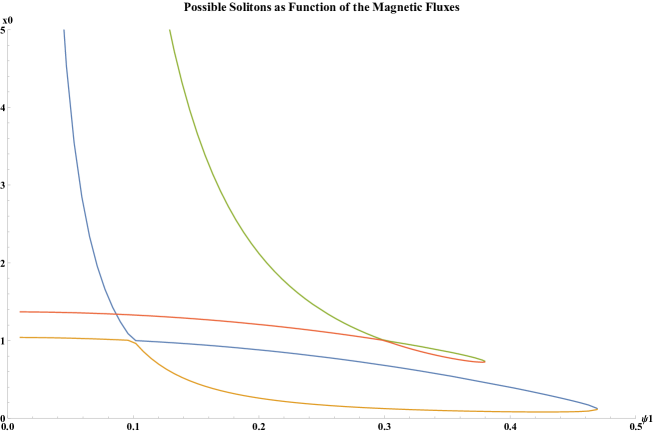
Figure 1: The different colors are different physical roots of (3.48). The $x_{0}$ in the $y$ axis are plotted vs the dimensionless Wilson line $\psi_{1}$ in the $x$-axis. The blue and yellow lines have $\psi_{2}=0.1$ and the red and green line have $\psi_{2}=0.3$. Either both solutions have a positive scalar field VEV or both have a negative scalar field VEV. The only roots that contribute to the physics are $x_{01}$ and $x_{03}$ (see Appendix A for their definition).

As we saw in (3.46), $T_{KK}=1/\delta$ defines the 3 dimensional gauge coupling, so fixing $\delta$ is like fixing the coupling constant in the UV. Then, since we are working at zero temperature, all the possible phase transitions are quantum critical phase transitions.

4 Holographic renormalization and a phase diagram

4.1 Holographic renormalization

Here we will use holographic renormalization to compute the expectation value of the dual energy momentum tensor. The countertems to deal with this situation were constructed in [18, 16, 19],

$$S=S_{0}+\frac{1}{\kappa}\int_{M^{3}\times S^{1}}K\sqrt{-h}d^{4}x+\frac{1}{2\kappa}\int_{M^{3}\times S^{1}}\sqrt{-h}\left(-\frac{6}{L}+\frac{1}{2L}\left(\frac{1}{\ln(\rho/\rho_{0})}-2\right)\Phi_{1}^{2}\right)d^{4}x\;,$$ (4.1)

where $S_{0}$ is the action (2.1) truncated to $\Phi_{2}=0$, $g_{\mu\nu}=h_{\mu\nu}+N_{\mu}N_{\nu}$, and $N_{\mu}$ is the outward pointing normal to the boundary and $K_{\mu\nu}=\frac{1}{2}\nabla_{\mu}N_{\nu}+\frac{1}{2}\nabla_{\nu}N_{\mu}$ is the extrinsic curvature. The boundary integrals are over the D3-brane geometry. Namely, a three dimensional Minkwoski spacetime times a circle,

$$ds^{2}=\gamma_{ab}dx^{a}dx^{b}=-dt^{2}+dy^{2}+dz^{2}+d\phi^{2}\;,$$ (4.2)

which is the background spacetime for the quantum field theory. The scalar field has in general the asymptotic expansion

$$\Phi_{1}=J_{\Phi}\frac{\ln(\rho^{2}/\rho_{0}^{2})}{\rho^{2}}+\frac{\Phi_{0}}{\rho^{2}}+O\left(\frac{\ln(\rho^{2}/\rho^{2}_{0})}{\rho^{4}}\right)\;,$$ (4.3)

with the on-shell variation

$$\frac{\delta S}{\delta J_{\Phi}}=\frac{1}{2\kappa L^{5}}\Phi_{0}.$$ (4.4)

Indeed, our soliton has no scalar sources and this relation provides the holographic interpretation of $\Phi_{0}$ as a VEV, as already explained. The vacuum expectation value of the energy momentum tensor of the dual field theory is

$$\left<T_{ab}\right> =\frac{-2}{\sqrt{-\gamma}}\frac{\delta S}{\delta\gamma^{ab}}$$ (4.5)

$$=\lim_{\rho\to\infty}\frac{\rho^{2}}{L^{2}}\frac{-2}{\sqrt{-h}}\frac{\delta S}{\delta h^{ab}}$$ (4.6)

$$=\lim_{\rho\to\infty}\frac{\rho^{2}}{L^{2}\kappa}\left(h_{ab}\;K-K_{ab}-\frac{3}{L}h_{ab}-\frac{1}{2L}h_{ab}\Phi_{1}^{2}\right)\;,$$ (4.7)

which yields

$$\left<T_{tt}\right>=-\frac{\mu}{2L^{3}\kappa}\;,\qquad\left<T_{zz}\right>=\left<T_{yy}\right>=\frac{\mu}{2L^{3}\kappa}\;,\qquad\left<T_{\phi\phi}\right>=-\frac{3\mu}{2L^{3}\kappa}\;.$$ (4.8)

4.2 Phase diagram from $E=E(\delta,\psi_{1},\psi_{2})$

The free energy of the solitons in the canonical ensemble is just the energy. Hence we will be interested to see how the the energy changes when we vary the sources $(\psi_{1},\psi_{2})$. A convenient normalization of the energy is that of the AdS Soliton [4],

$$E_{0}=-\frac{L^{3}\pi^{4}}{2\kappa\delta^{3}}V_{2}\;,$$ (4.9)

where $V_{2}$ is the volume of the $y-z$ plane. So we plot the energy of the solution with the running scalar $E_{\Phi}=\left<T_{tt}\right>V_{2}\delta$ divided by the absolute value of the energy of the AdS soliton in five dimensions,

$$F_{\Phi}\equiv\frac{E_{\Phi}}{|E_{0}|} =\left<T_{tt}\right>V_{2}\delta\frac{2\kappa\delta^{3}}{L^{3}\pi^{4}V_{2}}$$ (4.10)

$$=-16\frac{(\psi_{1}^{2}x_{0}^{2}-\psi_{2}^{2})(\psi_{1}^{2}x_{0}-\psi_{2}^{2})}{x_{0}(x_{0}-1)^{2}}\;,$$ (4.11)

We note that for the supersymmetric solution with $q_{1}=-q_{2}$, we have $\psi_{1}^{2}x_{0}^{2}-\psi_{2}^{2}=0=0$, so $F_{\Phi}=0$, as expected.

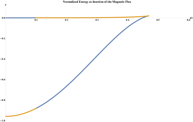
Figure 2: The normalized energy as a function of the Wilson line $\psi_{1}$ when $\psi_{2}=0.1$. The phase diagram is composed by the different D3-brane distributions. They turn out to be continuously connected on the gauge theory side due to the introduction of the Wilson lines in 5 dimensions. The different roots of the polynomial (3.50) have different colours.

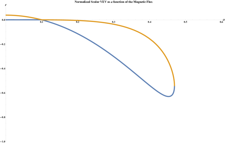
Figure 3: The normalized scalar field vacum expectation value as a function of the Wilson line $\psi_{1}$, when $\psi_{2}=0.1$. Here we see that the VEV is negative for some solutions and positive for others. The negative VEV yields D3 brane distributions different than the positive VEV, as we will discuss below. There is a crossover between the different regimes.

The free energy $F_{\Phi}$ changes its color in Fig.2 in a continuous way. At this point is possible to see that the scalar VEV continuously goes to zero indicating a redistribution of the D3-branes in the sense of [2]. This happens when $\psi_{2}=\pm\psi_{1}$. It is possible to see that the energy and all its derivatives are continuous at this point. That means that there is continuous phase transition at $\psi_{2}=\pm\psi_{1}$, generically followed by the phase transition at ($q_{1}=\pm q_{2}$, so) $|\psi_{2}|=x_{0}|\psi_{1}|<|\psi_{1}|$.

From $F(x_{0})=0$, meaning $\eta x_{0}^{2}=(x_{0}-1)^{2}(q_{1}^{2}-q_{2}^{2}x_{0})$, it is clear that we have the scalar VEV $\eta=0$ only for $q_{1}^{2}=q_{2}^{2}x_{0}$, meaning for $\psi_{1}^{2}x_{0}=\psi_{2}^{2}$, or for $x_{0}=1$, or for both, in which case we have $\psi_{1}=\pm\psi_{2}$ and $x_{0}=1$, where the horizon disappears (so there we transition between the "horizon" and "no horizon" phases, as we already explained). This is the "quantum phase transition" at $T_{KK}=0$ or $g^{2}_{\rm 3d,YM}=0$ described before.

The solution on the lower branch (with $F_{\Phi}<0$) increases $\psi_{i}$ until at some $\psi_{i}$, one reaches $F_{\Phi}=0$, corresponding to the supersymmetric solution ($q_{1}=-q_{2}$). There we have a phase transition to the phase dominated by the D3 brane distributions of [2] (which has zero energy), with anti-periodic boundary conditions for the fermions in $\phi$. From the point of view of the dual field theory, reduced on $\phi$ to 3 dimensions, this is another "quantum phase transition", at nonzero $g^{2}_{\rm 3d,YM}$. One should note however that the distributions of [2] are singular in the IR, so its inclusion in the phase diagram suppose that they actually become regular when quantum corrections are included.

4.3 QFT energy

Here we will discuss in greater detail how to understand the phase diagram from the QFT point of view. It is straightforward to compute the vacuum expectation value of the energy of a single scalar field in the background 4.2. The result is

$$\langle E_{\rm QFT}\rangle=-\frac{\pi^{2}}{6\delta^{3}}V_{2}X\;,$$ (4.12)

where $X$ is a numerical factor that depends whether the scalar field is periodic or anti-periodic in the $S^{1}$. It comes from Riemann zeta-function regularization of the sum over the modes in the circle and it yields

$$X_{even}=\sum_{n=1}^{\infty}(2n)^{3}=\frac{8}{120}\,,$$ (4.13)

$$X_{odd}=\sum_{n=1}^{\infty}(2n-1)^{3}=-\frac{7}{120}\,.$$ (4.14)

The field content of $\mathcal{N}=4$, $SU(N)$ super Yang-Mills is 6 scalars and 4 Weyl fermions in the adjoint representation plus one gauge vector. For the fermions the signs of the periodic and antiperiodic energies get interchanged. At weak coupling, we get the total energy by multiplying the scalar field energy by the number of degrees of freedom associated to each field, with the corresponding numerical factor depending on whether the fields are periodic or anti-periodic on the $S^{1}$. So for the case where the scalars, the vectors and the fermions are antiperiodic, we get

$$\langle E_{\rm SYM}\rangle=-\frac{\pi^{2}\,V_{2}}{6\delta^{3}}X_{odd}(N^{2}-1)(6+2-8)=0.$$ (4.15)

Hence this energy is automatically zero on account of the matching of the bosonic and fermionic degrees of freedom, and the fact that all fields have the same boundary condition on the $S^{1}$.

When the fermions are anti-periodic but the scalars and the vectors are periodic we get

$$\langle E_{\rm SYM*}\rangle=-\frac{\pi^{2}\,V_{2}}{6\delta^{3}}X_{even}(N^{2}-1)(6+2+8\frac{7}{8})=-\frac{\pi^{2}\,V_{2}}{6\delta^{3}}(N^{2}-1).$$ (4.16)

The AdS/CFT dictionary tell us that $\frac{L^{3}}{\kappa}=\frac{N^{2}}{4\pi^{2}}$. So the gravitational energy is

$$E_{0}=-\frac{\pi^{2}\,V_{2}}{8\delta^{3}}N^{2}=\frac{3}{4}\langle E_{\rm SYM*}\rangle\;,$$ (4.17)

which is a well-known result valid at large $N$. Thus, we learn that in our phase diagram is possible to see the interplay of $\langle E_{\rm SYM*}\rangle$ and $\langle E_{\rm SYM}\rangle$, and that morevoer, the value of $\langle E_{\rm SYM}\rangle$ at strong coupling and vanishing sources is also zero, see Fig. 2. This explains from the field theory point of view the existence of two branches of gravity solutions.

5 Continuous distributions of D3-branes vs. rotating D3-branes

We start by reviewing some of the findings of [2] on distributions of D3-branes. We show that when the gauge fields vanish in our soliton solutions, we recover the two different distributions of D3-branes that break the isometries of the $S^{5}$ to $SO(4)\times SO(2)$. The distribution of D3-branes of [2] are solutions of the supergravity action

$$I=\frac{1}{2\kappa}\int\sqrt{-g}\left(R-2\sum_{i=1}^{5}\left(\partial\alpha_{i}\right)^{2}-V\right)d^{5}x\;,$$ (5.1)

with

$$V = -\frac{1}{2L^{2}}\left[{\rm Tr}(M)^{2}-2{\rm Tr}(M^{2})\right],$$ (5.2)

$$M = diag(e^{2\beta_{1}},e^{2\beta_{2}},e^{2\beta_{3}},e^{2\beta_{4}},e^{2\beta_{5}},e^{2\beta_{6}}),$$ (5.3)

$$\vec{\beta} = \frac{1}{\sqrt{2}}B\vec{\alpha},$$ (5.4)

and

$$B=\begin{pmatrix}1&1&1&0&3^{-1/2}\\ 1&-1&-1&0&3^{-1/2}\\ -1&-1&1&0&3^{-1/2}\\ -1&1&-1&0&3^{-1/2}\\ 0&0&0&\sqrt{2}&-\frac{2}{3^{1/2}}\\ 0&0&0&-\sqrt{2}&-\frac{2}{3^{1/2}}\\ \end{pmatrix}.$$ (5.5)

Here $M$ is a representative of the coset $SL(6,\mathbb{R})/SO(6)$, and the action of $SO(6)$ on $M$ is by conjugation. Note that $B^{T}B=4\mathbb{1}_{5\times 5}$. Hence, the Lagrangian (5.1) is manifestly $SO(6)$ invariant.

The case $n=2$ of table 1 of [2] is recovered when $\vec{\alpha}=(0,0,0,0,-\frac{1}{2}\Phi)$ in terms of a canonically normalized scalar field $\Phi$, and then $\vec{\beta}=-\frac{\Phi}{2\sqrt{6}}(1,1,1,1,-2,-2)$. When the gauge fields vanish, this theory exactly coincides with the theory 2.1 when $\Phi=\Phi_{1}$. In the conventions of [2], this flow has $\Phi<0$, and therefore this corresponds in our coordinates to having $x<1$ and $\eta<0$.

The case $n=4$ of table 1 of [2] corresponds to $\vec{\alpha}=(\frac{\sqrt{3}}{4}\Phi,0,0,0,\frac{1}{4}\Phi)$ with the canonically normalized scalar field $\Phi$, and then $\vec{\beta}=\frac{\Phi}{2\sqrt{6}}(2,2,-1,-1,-1,-1)$. In this case we match their potential with $\Phi=\Phi_{1}$. This flow has $\Phi>0$, which in our coordinates is $x>1$ and $\eta>0$.

5.1 Uplift of the metric to 10 dimensions

For the purposes of top-down AdS/CFT (whose rules are derived from string theory), it is not enough to consider a 5-dimensional solution; rather, one has to have a 10-dimensional solution, moreover obtained from a D-brane configuration. This is possible in our case.

Indeed, using the uplift (2.3) we can write our solution, with non-vanishing gauge fields, as follows.

Considering the change of variable $x=\left(1+\epsilon\ell^{2}/r^{2}\right)^{-1}$ and using the uplift (2.3), we can write the 10-dimensional metric as

$$ds_{10}^{2} = \frac{\zeta(r,\theta)r^{2}}{L^{2}}\left(\frac{L^{2}dr^{2}}{r^{4}F(r)\lambda(r)^{6}}+dx_{1,2}^{2}+F\left(r\right)L^{2}d\phi^{2}\right)$$ (5.8)

$$+\frac{L^{2}}{\zeta(r,\theta)}\left\{\zeta(r,\theta)^{2}d\theta^{2}+\lambda(r)^{6}\sin^{2}\theta\left(d\phi_{3}+L^{-1}A_{3}\right)^{2}\right.$$

$$\left.+\cos^{2}\theta\left[d\psi^{2}+\sin^{2}\psi\left(d\phi_{1}+L^{-1}A_{1}\right)^{2}+\cos^{2}\psi\left(d\phi_{2}+L^{-1}A_{2}\right)^{2}\right]\right\}\ ,$$

$$F\left(r\right) = L^{-2}+\frac{\ell^{4}}{\eta r^{4}}\left(q_{1}^{2}-q_{2}^{2}\lambda(r)^{-6}\right)\ ,\qquad\lambda(r)^{6}=1+\epsilon\frac{\ell^{2}}{r^{2}}\ ,\qquad\zeta(r,\theta)^{2}=1+\epsilon\frac{\ell^{2}}{r^{2}}\cos^{2}\theta\;,$$ (5.9)

$$A_{1} = A_{2}=\epsilon q_{1}\ell^{2}\frac{r^{2}-r_{0}^{2}}{r^{2}r_{0}^{2}}Ld\phi\;,\qquad A_{3}=\epsilon q_{2}\ell^{2}\frac{r^{2}-r_{0}^{2}}{(r^{2}+\epsilon\ell^{2})(r_{0}^{2}+\epsilon\ell^{2})}Ld\phi\;,$$ (5.10)

where $\epsilon=\pm 1$ depending whether the scalar is positive or negative, and $r_{0}$ is the zero of $F(r)$. For consistency, $\eta$ and $\epsilon$ must have opposite signs, hence we considered $\eta=-\epsilon\ell^{2}/L^{2}$. We use $\vec{\mu}=\left(\cos\theta\sin\psi,\cos\theta\cos\psi,\sin\theta\right)$. The field strength 5-form $F_{5}=G_{5}+\star G_{5}$ is defined in terms of $G_{5}$ given by

$$G_{5} = \frac{2r^{3}\epsilon}{L^{4}\lambda^{6}}\left[\sin^{2}\theta+\lambda^{12}\cos^{2}\theta-\zeta^{2}\left(1+2\lambda^{6}\right)\right]dr\wedge dt\wedge dy\wedge dz\wedge d\phi$$

$$-\frac{\epsilon\lambda^{\prime}r^{3}}{\lambda L^{2}}\left[2r^{2}\lambda^{6}F\left(r\right)+3L^{2}\left(1-\lambda^{6}\lambda_{0}^{-6}\right)\left(q_{2}^{2}-q_{1}^{2}\lambda^{6}\lambda_{0}^{6}\right)\right]\sin\left(2\theta\right)d\theta\wedge dt\wedge dy\wedge dz\wedge d\phi$$

$$+3r^{3}\epsilon\lambda^{5}\lambda^{\prime}\left[\sin\left(2\theta\right)d\theta\wedge\left(q_{1}\sin^{2}\psi d\phi_{1}+q_{1}\cos^{2}\psi d\phi_{2}+q_{2}d\phi_{3}\right)\right.$$

$$\left.-q_{1}\cos^{2}\theta\sin\left(2\psi\right)d\psi\wedge\left(d\phi_{1}-d\phi_{2}\right)\right]\wedge dt\wedge dy\wedge dz\ .$$

The field strength 5-form can be written explicitly as the exterior derivative of a 4-form as $F_{5}=d(\mathcal{C}_{4}+\tilde{\mathcal{C}}_{4})$, where

$$\mathcal{C}_{4} = -\left[\frac{r^{4}}{L^{4}}\zeta(r,\theta)^{2}+\frac{\ell^{4}}{r_{0}^{2}}\epsilon\cos^{2}\theta(q_{2}^{2}\lambda(r_{0})^{-6}-q_{1})\right]dt\wedge dy\wedge dz\wedge d\phi$$

$$+\ell^{2}\epsilon(q_{1}\cos^{2}\theta(\cos^{2}\psi d\phi_{2}+\sin^{2}\psi d\phi_{1})+q_{2}\cos^{2}\theta d\phi_{3})\wedge dt\wedge dy\wedge dz\,$$

$$\tilde{\mathcal{C}}_{4} = \frac{L^{4}r^{2}\lambda(r)^{6}\cos^{4}\theta\sin(2\psi)}{2r^{2}\zeta(r,\theta)^{2}}d\phi_{1}\wedge d\phi_{2}\wedge d\phi_{3}\wedge d\psi$$

$$-\frac{L^{4}q_{2}r^{2}(\lambda(r)^{6}-\lambda(r_{0})^{6})}{r^{2}\zeta(r,\theta)^{2}\lambda(r_{0})^{6}}\cos^{4}\theta\cos\psi\sin\psi d\phi\wedge d\phi_{1}\wedge d\phi_{2}\wedge d\psi$$

$$-\frac{\ell^{2}L^{4}q_{1}r\epsilon\cos(2\psi)\sin^{2}(2\theta)}{8r^{4}\zeta(r,\theta)^{4}}(1+\frac{\epsilon\ell^{2}}{r_{0}^{2}}\cos^{2}\theta)dr\wedge d\phi\wedge\phi_{3}\wedge(d\phi_{1}-d\phi_{2})$$

$$-\frac{L^{4}r^{4}q_{1}\ell^{2}\epsilon\sin(2\theta)}{4r^{6}\zeta(r,\theta)^{4}}d\theta\wedge d\phi\wedge d\phi_{3}\wedge$$

$$\left[-\zeta(r,\theta)^{4}(d\phi_{1}+d\phi_{2})+r^{2}\lambda(r)^{6}(r^{-2}-r_{0}^{-2})\cos(2\psi)\cos^{2}\theta(d\phi_{1}-d\phi_{2})\right]$$

with $G_{5}=d\mathcal{C}_{4}$, $*G_{5}=d\tilde{\mathcal{C}}_{4}$.

The flux of the $F_{5}$ on the $S^{5}$ with coordinates $[\theta,\psi,\phi_{1},\phi_{2},\phi_{3}]$ and ranges $\theta,\psi\in[0,\pi/2]$, $\phi_{1},\phi_{2},\phi_{3}\in[0,2\pi]$ is given by

$$\int_{S^{5}}F_{5}=\int_{S^{5}}\star F_{5}=\epsilon 4\pi^{3}L^{4}\,.$$ (5.14)

Regarding the supersymmetry of the configuration, we show that the determinant of the components of integrability conditions (2.33) are all zero for $|q_{1}|=|q_{2}|$, which ensures the existence of a solution of the Killing spinor equation (2.32). Consequently, from the point of view of IIB supergravity, the Killing spinor equation admits a solution even in the case $q_{1}=q_{2}$, in addition to the case $q_{1}=-q_{2}$ that we found in $D=5$.

5.2 Mass spectrum and phase transitions

In the case $A^{i}=0$ of [2], it was noted that for the dilaton, one can reduce the 10-dimensional equation of motion onto the 5-dimensional one, if we have a warped product form,

$$ds^{2}_{10}=\Delta^{-2/3}(r,\mu_{i},\phi_{i})ds^{2}_{5}(y,z,t,r,\phi)+ds^{2}_{K}(\mu_{i},\phi_{i},r)\;,$$ (5.15)

so $ds_{K}$ that can depend on $ds_{5}$, but $ds_{5}$ independent on $ds_{K}$, and if the dilaton is independent on $K$, so $\Phi=\Phi(t,y,z,r,\phi)$. Here $\Delta=\sqrt{\det g_{K}/\det g_{K}^{(0)}}$, where $g_{K}^{(0)}$ is the metric of the undeformed by $ds_{5}$ metric of $K$, i.e., in this case, the metric of the round $S^{5}$ sphere, and $g_{K}$ is the full deformed metric on $K$.

That is so, since we can easily verify that the 10-dimensional d’Alembertian operator on $\Phi$ is

$$\Box_{10D}\Phi=\frac{\Delta^{2/3}}{\sqrt{-g}}{\partial_{\mu}(g^{\mu\nu}\sqrt{-g}\partial_{\nu}\Phi)}+ds_{K}\;terms\,,$$ (5.16)

where $g_{\mu\nu}$ is the 5-dimensional metric for $ds_{5}$. Hence, this is equivalent to solving the d’Alembertian (massless KG) equation in the 5-dimensional metric $ds_{5}^{2}$.

In our case, with $A^{i}\neq 0$, specifically $g_{\phi K}\neq 0$, we have the same situation, if we impose the additional constraint that $\Phi$ is independent on the circle (KK) coordinate $\phi$, so $\Phi=\Phi(t,y,z,r)$ only, in which case we have the same 5-dimensional $\Box$ operator, but acting on a field that only depends on 4 dimensions, so on the zero mode for the KK expansion on $S^{1}$.

By comparing this form with our own uplift form (2.3), we see that

$$\tilde{\Delta}^{1/2}=\Delta^{-2/3}=\frac{\zeta(r,\theta)}{\lambda^{2}(r)}\;,$$ (5.17)

which means that the 5-dimensional metric in our case can be put into the form

$$ds^{2}_{5} = \frac{\lambda^{2}r^{2}}{L^{2}}\left(\frac{L^{2}dr^{2}}{r^{4}F(r)\lambda^{6}}+d\vec{x}^{2}_{1,2}+F(r)L^{2}d\phi^{2}\right)$$ (5.18)

$$= \frac{r^{2}}{L^{2}}\left(1+\epsilon\frac{\ell^{2}}{r^{2}}\right)^{1/3}\left[\frac{L^{d}r^{2}}{r^{4}F(r)\left(1+\epsilon\frac{\ell^{2}}{r^{2}}\right)}+d\vec{x}^{2}_{1,2}+F(r)L^{2}d\phi^{2}\right]\;,$$ (5.19)

and by using redefining $r/L=L/z$, we have

$$ds_{5}^{2}=\frac{L^{2}}{z^{2}}\left(1+\epsilon\frac{\ell^{2}z^{2}}{L^{4}}\right)^{1/3}\left[\frac{dz^{2}}{L^{4}F(z)\left(1+\epsilon\frac{\ell^{2}z^{2}}{L^{4}}\right)}+d\vec{x}_{1,2}^{2}+F(z)L^{2}d\phi^{2}\right]\;,$$ (5.20)

with

$$F(z)=1-\epsilon\frac{\ell^{2}z^{4}}{L^{6}}\left(q_{1}^{2}-\frac{q_{2}^{2}}{1+\epsilon\frac{\ell^{2}z^{2}}{L^{4}}}\right).$$ (5.21)

Then the spectrum of the scalar $0^{++}$ glueballs is given by the eigenstates of the d’Alembertian operator in this 5-dimensional background. Since

$$\Box\Phi=\frac{z^{5}}{\left(1+\epsilon\frac{\ell^{2}z^{2}}{L^{4}}\right)^{1/3}}\partial_{z}\left[\frac{\left(1+\epsilon\frac{\ell^{2}z^{2}}{L^{4}}\right)}{z^{3}}F(z)\partial_{z}\right]\Phi+\frac{z^{2}}{\left(1+\epsilon\frac{\ell^{2}z^{2}}{L^{4}}\right)^{1/3}}\partial_{i}\partial_{i}\Phi\;,$$ (5.22)

under the redefinition of the variable, $dz=\sqrt{F(z)\left(1+\epsilon\frac{\ell^{2}z^{2}}{L^{4}}\right)}du$, and of the function, with a $e^{i\vec{k}\cdot\vec{x}}$ plane wave in the $y,z,t$ directions, and with $\vec{k}^{2}=-M^{2}$,

$$\Phi=e^{i\vec{k}\cdot\vec{x}}\frac{z^{3/2}}{F(z)\left(1+\epsilon\frac{\ell^{2}z^{2}}{L^{4}}\right)}\Psi(z)\;,$$ (5.23)

from $\Box\Phi=0$ we get the one-dimensional Schrödinger equation,

$$-\frac{d^{2}\Psi(u)}{du^{2}}+V(u)=M^{2}\Psi(u)$$ (5.24)

$$V(z)=-\left[F(z)\left(1+\epsilon\frac{\ell^{2}z^{2}}{L^{4}}\right)\right]^{1/4}z^{3/2}\frac{d}{dz}\left\{\frac{F(z)\left(1+\epsilon\frac{\ell^{2}z^{2}}{L^{4}}\right)}{z^{3}}\frac{d}{dz}\frac{z^{3/2}}{\left[F(z)\left(1+\epsilon\frac{\ell^{2}z^{2}}{L^{4}}\right)\right]^{1/4}}\right\}.$$ (5.25)

We see that we can redefine $\tilde{F}(z)\equiv F(z)\left(1+\epsilon\frac{\ell^{2}z^{2}}{L^{4}}\right)$, in which case we are back to the case considered in [20].

We can now make the same analysis from before (in 5 dimensions, in terms of the $x$ coordinate) for the $z_{0}$ solving $F(z_{0})=0$, but now also consider together with the one solving $\tilde{F}(z_{0})=0$, which is more relevant:

-if $\epsilon=+1$, $q_{2}\rightarrow 0$ gives an $z_{0}$, but $q_{1}=0$ gives no $z_{0}$ (but $q_{1}\rightarrow 0$, yet $q_{1}\neq 0$, gives an $z_{0}$).

-if $\epsilon=-1$, $q_{2}=0$ gives no $z_{0}$ (but $q_{2}\rightarrow 0$, yet $q_{2}\neq 0$, gives an $z_{0}$), but $q_{1}\rightarrow 0$ gives an $z_{0}$.

-if $q_{1}=\pm q_{2}$ (in the susy case), there always is an $z_{0}$.

-if $\epsilon=-1$, $q_{2}=0$, there is no solution to $F(z_{0})=0$, but there is a solution to $\tilde{F}(z)=0$, namely $z_{0}=L^{2}/\ell$.

-if $\epsilon=+1$ and $q_{1}=q_{2}=0$, we get no $z_{0}$.

In the UV, at $z\rightarrow 0$, we have $\tilde{F}(z)\simeq 1$, so we get $z\simeq u$ and the same potential for both $\epsilon=\pm 1$,

$$V(u\simeq 0)\simeq\frac{15}{4u^{2}}\Rightarrow\Psi(u)=\sqrt{Mu}\left[C_{1}J_{2}(Mu)+C_{2}Y_{2}(Mu)\right].$$ (5.27)

In the IR, we can have a $z_{0}\neq 0$, or not, as we discussed, depending on $\epsilon,\ell$ and $q_{1},q_{2}$.

If we have a $z_{0}\neq 0$, then for $z\rightarrow z_{0}$, with $\tilde{F}(z)\simeq\tilde{F}^{\prime}(z_{0})(z-z_{0})$, $u-u_{\rm max}\simeq 2\sqrt{(z-z_{0})/\tilde{F}^{\prime}(z_{0})}$, and writing $u_{\rm max}=Kz_{0}$, we get

$$V(u\simeq Kz_{0}) \simeq -\frac{\tilde{F}^{\prime}(z_{0})}{16|z-z_{0}|}\simeq-\frac{1}{4(u-Kz_{0})^{2}}\Rightarrow$$ (5.28)

$$\Psi \simeq \sqrt{Kz_{0}-u}\left[C^{\prime}_{1}J_{0}\left(M(u-Kz_{0})\right)+C^{\prime}_{2}Y_{0}\left(M(u-Kz_{0})\right)\right].$$ (5.29)

The IR boundary condition puts $C^{\prime}_{2}=0$, so the $J_{0}$ solution continued to the UV (at $u=0$) must give also $C_{2}=0$, which will give a quantization condition on $M(Kz_{0})=Mu_{\rm max}$, as $M=M_{n}$. But, of course, the quantization condition will depend on the parameters $(q_{1},q_{2},\ell)$ of the solution, which will define $u_{\rm max}$, decoupling the scale of $M_{n}$, $u_{\rm max}$, from the KK scale, $T_{\rm KK}=1/\delta$. In any case, the spectrum is discrete.

On the other hand, if there is no $z_{0}$ (so $z_{0}=0$) in the IR,

-if $\epsilon=+1,q_{1}=0$, then $\tilde{F}(z)\sim(q_{2}^{2}\ell^{2}/L^{6})z^{4}$, so

$$V(z\rightarrow\infty)\simeq-\frac{1}{4}z^{2}\frac{q_{2}^{2}\ell^{2}}{L^{6}}\simeq-\frac{1}{4(u-u_{\rm max})^{2}}\;,$$ (5.30)

so, despite the fact that we don’t have a $z_{0}$, we obtain the same form of the potential in terms of $u$, since $\int du\simeq 1/\sqrt{(q_{2}^{2}\ell^{2}/L^{6})z^{2}}$. So again a discrete spectrum.

-if $\epsilon=-1,q_{2}=0$, then there is no $z_{0}$ for $F(z)$, but there is one for $\tilde{F}(z)$, so the solution is again the same as before, and we have a discrete spectrum.

-if $\epsilon=+1,q_{1}=q_{2}=0$, then there is no $z_{0}$ for $F(z)$ or $\tilde{F}(z)$, and then $\tilde{F}(z)\simeq\ell^{2}z^{/}L^{4}$, so

$$V(z\rightarrow\infty)\simeq+\frac{\ell^{2}}{L^{4}}=V(u)\;,$$ (5.31)

so we have a continuous spectrum above a mass gap at $M^{2}=\ell^{2}/L^{4}$.

In conclusion, this case of $\epsilon=+1,q_{1}=q_{2}=0$ is the only one for which we have a qualitatively different spectrum.

We can then say that the introduction of the $q_{1},q_{2}$ charges induces a phase transition from the spectrum continuous above a mass gap, continuously connected to the discrete spectrum. At $q_{1}=q_{2}=0$, the two spectra seemed distinct, as they were obtained in the two separate cases, $\epsilon=+1$ and $\epsilon=-1$, respectively.

Finally, when we have the pure AdS space, obtained formally by putting $F(z)=1,\ell=0$, we obtain that the potential in the UV is valid everywhere, $u=z$ and $V(z)=\frac{15}{4u^{2}}$. In this case, there is no limit on $u=z$, it spans from $u=0$ to $u=+\infty$, which means that the spectrum is continuous without a mass gap.

Since, as we saw in section 4, we had two phase transitions, interpreted as quantum phase transitions from the point of view of the 3-dimensional dual field theory reduced on $\phi$, one from "no horizon" (given by the singular distributions of D3 branes) to "horizon" (at $g^{2}_{\rm 3d,YM}=0$), and then to "AdS space" (at $g^{2}_{\rm 3d,YM}\neq 0$), these are: from continuous above a mass gap to discrete, to continuous without a mass gap.

6 Discussion and conclusions

In this paper we have found AdS solitons depending on three parameters, namely the two sources associated to the gauge fields, which were proportional to the charge parameters $q_{1},q_{2}$, and the value of the periodicity of the circle $S^{1}$, $\delta$. We have shown that it is possible to describe the phase space in terms of the dimensionless sources $(\psi_{1},\psi_{2})$, together with $\delta=1/T_{\rm KK}$. The solutions give a dual scalar VEV $\langle{\cal O}\rangle_{(1,1)_{0}}$ in 3+1 dimensions, proportional to $\eta=\pm\ell^{2}/L^{2}$. Among the solutions, a special role is played by the supersymmetric solutions, with $q_{1}=\pm q_{2}$.

We have found two phase transitions from the $(E,\psi_{1},\psi_{2})$ diagram, as $\psi_{1}$ is varied, one at $\psi_{1}=\pm\psi_{2},x_{0}=1$, and another the one at $\psi_{2}=\pm\psi_{1}x_{0}(\psi_{1},\psi_{2})$ and $E=0$, to the previous solutions of [2].

Our set of solutions continuously connects all the possibilities described in [2]. The 10-dimensional uplift of the solutions was found to be a deformation of the D3-brane distributions of [2], and in the appendix below we hint towards its description as a system of D3-branes, obtained from the Wick rotation of the rotating D3-branes in 3 independent planes, so one expects that there is a good string theory interpretation of the results, though we have not found it so far.

In terms of the 2+1-dimensional interpretation, the supersymmetric solutions give a quantum critical phase transition, at $g^{2}_{\rm 3d,YM}=0$, between a phase with no VEV (and no horizon in the dual), and spectrum that is continuous above a mass gap, and a phase with VEV (and horizon in the dual), and discrete spectrum, and the transition to periodic AdS space is to a continuous and no mass gap spectrum, at nonzero $g^{2}_{\rm 3d,YM}$.

Remarkably enough, we have found that the phase diagram of these solutions should correspond to the strongly coupled description of the existence of two possible vacua of the large $N$ $\mathcal{N}=4$ SYM when compactified on an $S^{1}$ in four dimensions and antiperiodic boundary conditions for the fermions on the $S^{1}$. Unexpectedly, we found that at finite values of the source the supersymmetry breaking vacuum gets its supersymmetry restored, corresponding to the BPS states existing in supergravity.

Hence, this should correspond to the existence to a non-perturbative object in the field theory, most likely the Q-ball [21], embedded into the supersymmetric theory, and extended to strong coupling (where its stability properties and mass value with respect to the ones fundamental fields are not currently understood). Indeed, we see that in the UV, at $x=1$, we have $A^{1}=A^{2}=q_{1}(1-x_{0}^{-1})Ld\phi$, $A^{3}=q_{2}(1-x_{0})Ld\phi$.

In the case of the double Wick rotation of the solution, with $F(x)$ multiplying $-dt^{2}$ instead of $d\phi^{2}$ in the metric, this would give $A^{1}=A^{2}=q_{1}(1-x_{0}^{-1})Ldt$, $A^{3}=q_{2}(1-x_{0})Ldt$, which is the standard case for $\mu_{1}=q_{1}(1-x_{0}^{-1})L$, $\mu_{2}=q_{2}(1-x_{0})L$, chemical potentials, or sources, for the corresponding $U(1)$ charges $\int d^{3}x\;\rho$, where $\rho\sim{\rm Tr}[\bar{Z}\partial^{0}Z]+{\rm Tr}[\bar{\psi}\gamma^{0}\psi]$, with $Z$ complex combinations of $X^{I}$’s, and $\psi$ complex fermions, both charged under the $U(1)$’s.

Therefore in our case, $A^{1}=A^{2}=q_{1}(1-x_{0}^{-1})Ld\phi$ and $A^{3}=q_{2}(1-x_{0})Ld\phi$, $\mu_{1}$ and $\mu_{2}$ are sources for the $U(1)$ current components in the $\phi$ direction, $\sim{\rm Tr}[\bar{Z}\partial^{\phi}Z]+{\rm Tr}[\bar{\psi}\gamma^{\phi}\psi]$, so they are understood as $J^{\phi}=\rho v^{\phi}=\rho\frac{d\phi}{dt}\equiv\rho\omega$ (if we had $\rho\vec{v}$, we would write $Z=Z(\vec{x}-\vec{v}t)$, with $\vec{x}=(y,z)$). We see that, from the point of view of the reduced 2+1 dimensional theory in $(t,y,z)$, in which $\phi$ is an internal direction, $\omega$ might be understood as Q-ball [21] angular frequency (for effective potential $V_{\rm eff}(Z)=V+\frac{1}{2}\omega^{2}|Z|^{2}$), for writing $Z(\phi=\omega t,\vec{x})=e^{i\omega t}Z(\vec{x})$, and $J^{\phi}$ is then Q-ball charge density (except, of course, that we don’t have a time dependence of the phase $\phi$, that was just assumed). Then $\mu_{1},\mu_{2}$ would be chemical potentials for the Q-ball charges.

This might provide a generalization of the Coulomb Branch solution for ${\cal N}=4$ SYM, by the parameters $\eta$ (operator VEV) and $q_{1},q_{2}$ (related to the $\mu_{1},\mu_{2}$, the "chemical potentials for Q-ball charges"), that contains both solutions with arbitrary (or no) periodicity of $\phi$, better understood within ${\cal N}=4$ SYM, and solutions with periodic $\phi$ and cigar-type solution with an $x_{0}$ ("horizon"), understood either from the point of view of the reduction to 3 dimensions ($(y,z,t)$), or from the point of view of Euclidean version of 4 dimensions, at finite KK temperature $T_{\rm KK}$. We expect to make this picture more concrete in a future work.

Appendix A Solutions of the cubic equation (3.50)

The solutions of (3.50) have the form $x_{0i}=\lambda_{1}\cos\left(\Theta+\frac{2\pi n_{i}}{3}\right)-\frac{\lambda_{2}}{3}$ with $n_{i}=0,1,2$ for $i=1,2,3$, and

$$\lambda_{1}= \frac{2}{3\psi_{1}}\sqrt{8\psi_{1}^{4}\lambda_{2}-\psi_{1}^{2}\lambda_{2}^{2}-8\psi_{2}^{2}\psi_{1}^{2}\lambda_{2}+2\psi_{2}^{4}\lambda_{2}+12\psi_{2}^{2}\psi_{1}^{2}-2\psi_{2}^{2}\lambda_{2}-2\psi_{1}^{2}\lambda_{2}-3\psi_{2}^{2}-6\psi_{2}^{4}}\;,$$ (A.1)

$$\lambda_{2}= \frac{1}{\psi_{1}^{2}}\left(-4\psi_{2}^{2}\psi_{1}^{2}+\psi_{2}^{4}+4\psi_{1}^{4}-\psi_{2}^{2}-\psi_{1}^{2}\right)\;,$$ (A.2)

$$\Theta= 3^{-1}\arccos{\frac{4}{27\lambda_{1}^{3}\psi_{1}^{2}}\left(3\psi_{2}^{2}\lambda_{2}^{2}+3\psi_{1}^{2}\lambda_{2}^{2}+9\psi_{2}^{2}\lambda_{2}+18\psi_{2}^{4}\lambda_{2}-12\psi_{1}^{4}\lambda_{2}^{2}-27\psi_{2}^{4}+12\psi_{2}^{2}\psi_{1}^{2}\lambda_{2}^{2}\right.}$$ (A.3)

$$\left.-3\psi_{2}^{4}\lambda_{2}^{2}-36\psi_{2}^{2}\psi_{1}^{2}\lambda_{2}+\psi_{1}^{2}\lambda_{2}^{3}\right).$$ (A.4)

Appendix B Integrability conditions

In this appendix we compute the integrability condition for IIB in the metric-$F_{5}$ sector. The supersymmetry transformations of the spin 3/2 field is

$$\delta\psi_{\mu}dx^{\mu}=d\epsilon+W\epsilon\equiv D\epsilon\ ,$$ (B.1)

where for our field content

$$W=\frac{1}{4}\omega_{ab}\Gamma^{ab}+\frac{1}{16}i\sigma_{2}\not{F}_{5}\Gamma_{a}e^{a}\ .$$ (B.2)

We define integrability conditions $2-$form as the commutator of the covariant derivative defined in (B.1)

$$\Xi\equiv D\wedge D\epsilon\ .$$ (B.3)

It is simple to show that

$$\Xi=dW+W\wedge W\ .$$ (B.4)

Let us compute it term by term. The exterior derivative of $W$ is

$$dW=\frac{1}{4}d\omega_{ab}\Gamma^{ab}+\frac{1}{16}i\sigma_{2}d\not{F}_{5}\Gamma_{a}e^{a}+\frac{1}{16}i\sigma_{2}\not{F}_{5}\Gamma_{a}de^{a}\ .$$ (B.5)

Using the torsion-less condition $de^{a}+\omega_{\ b}^{a}\wedge e^{b}=0$ and the definition of curvature $2-$form $R_{\ b}^{a}=\omega_{\ b}^{a}+\omega_{\ c}^{a}\wedge\omega_{\ b}^{c}$ we obtain

$$dW=\frac{1}{4}R_{ab}\Gamma^{ab}-\frac{1}{4}\omega_{ac}\wedge\omega_{\ b}^{c}\Gamma^{ab}+\frac{1}{16}i\sigma_{2}d\not{F}_{5}\Gamma_{a}e^{a}-\frac{1}{16}i\sigma_{2}\not{F}_{5}\Gamma_{a}\omega_{\ c}^{a}\wedge e^{c}\ .$$ (B.6)

Note that in general one can write $W=W_{A}\otimes\Gamma^{A}$ where $W_{A}$ is the tensor product of the 1-form space and $2\times 2$ matrices, in general we suppress the tensor product symbol. The repeated indices $A$ are sumed over all terms which defines $W$ and encodes the index structure of the $\Gamma$ matrices in each term. Using this, we have

$$W\wedge W=\frac{1}{2}W_{A}\wedge W_{B}\left[\Gamma^{A},\Gamma^{B}\right]\ .$$ (B.7)

A general identity of the $\Gamma$ matrices that we will use are

$$\Gamma^{a_{1}\dots a_{p}}\Gamma_{bc} = \Gamma^{a_{1}\dots a_{p}}{}_{bc}-2p\Gamma^{[a_{1}\dots a_{p-1}}{}_{[b}\delta_{c]}^{a_{p}]}-\frac{p!}{\left(p-2\right)!}\Gamma^{[a_{1}\dots a_{p-2}}\delta_{[b}^{a_{p-1}}\delta_{c]}^{a_{p}]}\ ,$$ (B.8)

$$\Gamma_{bc}\Gamma^{a_{1}\dots a_{p}} = \Gamma_{ab}{}^{a_{1}\dots a_{p}}-2p\delta_{[b}^{[a_{1}}\Gamma_{c]}^{a_{2}\dots a_{p}]}-\frac{p!}{\left(p-2\right)!}\delta_{[b}^{[a_{1}}\delta_{c]}^{a_{2}}\Gamma^{a_{3}\dots a_{p}]}\ .$$ (B.9)

In particular, we can derive from it

$$\left[\Gamma^{ab},\Gamma_{c}\right] = 4\Gamma^{[a}\delta_{c}^{b]}\ ,\qquad\left[\Gamma^{ab},\Gamma_{cd}\right]=8\delta_{[a}^{[c}\Gamma^{d]}{}_{b]}\ ,$$ (B.10)

$$\left[\Gamma^{a_{1}a_{2}a_{3}a_{4}a_{5}},\Gamma_{bc}\right] = -20\Gamma_{[b}{}^{[a_{1}a_{2}a_{3}a_{4}}\delta_{c]}^{a_{5}]}\ .$$

Replacing (B.2) into (B.7) we get

$$W\wedge W = \frac{1}{2}\frac{1}{4}\omega_{ab}\wedge\frac{1}{4}\omega_{cd}\left[\Gamma^{ab},\Gamma^{cd}\right]+\frac{1}{8^{2}}i\sigma_{2}\omega_{ab}\wedge e^{c}\frac{1}{5!}F_{d_{1}\dots d_{5}}\left[\Gamma^{ab},\Gamma^{d_{1}\dots d_{5}}\Gamma_{c}\right]$$ (B.11)

$$-\frac{1}{8^{3}}\left[\not{F}_{5}\Gamma_{a},\not{F}_{5}\Gamma_{c}\right]e^{a}\wedge e^{c}\ .$$

Using the commutator relations, we obtain

$$W\wedge W = \frac{1}{4}\omega_{ac}\wedge\omega_{\ b}^{c}\Gamma^{ab}+\frac{1}{2}\frac{1}{8}i\sigma_{2}\omega_{\ b}^{a}\wedge e^{b}\not{F}_{5}\Gamma_{a}-\frac{1}{2}\frac{1}{8}i\sigma_{2}\omega^{ab}\wedge e^{c}\frac{1}{4!}F_{d_{1}\dots d_{4}b}\Gamma^{d_{1}\dots d_{4}}{}_{a}\Gamma_{c}$$ (B.12)

$$-\frac{1}{8^{3}}\left[\not{F}_{5}\Gamma_{a},\not{F}_{5}\Gamma_{c}\right]e^{a}\wedge e^{c}\ .$$

Replacing (B.6) and (B.7) into (B.4), the $2-$form integrability conditions become

$$\Xi = \frac{1}{4}R_{ab}\Gamma^{ab}+\frac{1}{16}i\sigma_{2}\frac{1}{5!}dF_{b_{1}\dots b_{5}}\Gamma^{b_{1}\dots b_{5}}\Gamma_{a}e^{a}-\frac{1}{2}\frac{1}{8}i\sigma_{2}\omega^{ab}\wedge e^{c}\frac{1}{4!}F_{d_{1}\dots d_{4}b}\Gamma^{d_{1}\dots d_{4}}{}_{a}\Gamma_{c}$$ (B.13)

$$-\frac{1}{8^{3}}\left[\not{F}_{5}\Gamma_{a},\not{F}_{5}\Gamma_{c}\right]e^{a}\wedge e^{c}\ .$$

Note that the second and third term form a Lorentz covariant derivative

$$\Xi=\frac{1}{4}R_{ab}\Gamma^{ab}+\frac{1}{16}i\sigma_{2}\frac{1}{5!}\mathcal{D}F_{b_{1}\dots b_{5}}\Gamma^{b_{1}\dots b_{5}}\Gamma_{a}e^{a}-\frac{1}{8^{3}}\left[\not{F}_{5}\Gamma_{a},\not{F}_{5}\Gamma_{c}\right]e^{a}\wedge e^{c}\ .$$ (B.14)

The last term can be simplified by using $\left[\Gamma^{d_{1}\dots d_{5}},\Gamma_{a}\right]=2\Gamma^{d_{1}\dots d_{5}}{}_{a}$, then

$$\left[\not{F}_{5}\Gamma_{a},\not{F}_{5}\Gamma_{c}\right]e^{a}\wedge e^{c}=4\not{F}_{5}\frac{1}{4!}F_{ab_{1}\dots b_{4}}\Gamma^{b_{1}\dots b_{4}}\Gamma_{c}e^{a}\wedge e^{c}-2\not{F}_{5}\not{F}_{5}\Gamma_{ac}e^{a}\wedge e^{c}\ .$$ (B.15)

The last term of (B.15) vanishes due to the fact that $F_{5}$ is self-dual,

$$\left(5!\right)^{2}\not{F}_{5}\not{F}_{5} = F_{a_{1}\dots a_{5}}F_{b_{1}\dots b_{5}}\Gamma^{a_{1}\dots a_{5}}\Gamma^{b_{1}\dots b_{5}}\ ,$$

$$\sim F^{d_{1}\dots d_{5}}\epsilon_{a_{1}\dots a_{5}d_{1}\dots d_{5}}F_{c_{1}\dots c_{5}}\epsilon^{c_{1}\dots c_{5}b_{1}\dots b_{5}}\Gamma^{a_{1}\dots a_{5}}\Gamma_{b_{1}\dots b_{5}}\ ,$$

$$= F^{d_{1}\dots d_{5}}F_{c_{1}\dots c_{5}}\delta_{a_{1}\dots a_{5}d_{1}\dots d_{5}}^{c_{1}\dots c_{5}b_{1}\dots b_{5}}\Gamma^{a_{1}\dots a_{5}}\Gamma_{b_{1}\dots b_{5}}\ ,$$

$$= F^{d_{1}\dots d_{5}}F^{a_{1}\dots a_{5}}\delta_{c_{1}\dots c_{5}d_{1}\dots d_{5}}^{a_{1}\dots a_{5}b_{1}\dots b_{5}}\Gamma_{a_{1}\dots a_{5}}\Gamma_{b_{1}\dots b_{5}}\;.$$

Now we can anti-symmetrize and construct a $\Gamma_{a_{1}\dots a_{10}}$, and then use the fact that it is proportional to $\epsilon_{a_{1}\dots a_{10}}\Gamma_{11}$,

$$\left(5!\right)^{2}\not{F}_{5}\not{F}_{5} = F^{d_{1}\dots d_{5}}F^{a_{1}\dots a_{5}}\delta_{c_{1}\dots c_{5}d_{1}\dots d_{5}}^{a_{1}\dots a_{5}b_{1}\dots b_{5}}\Gamma_{a_{1}\dots a_{5}b_{1}\dots b_{5}}\ ,$$

$$\sim F^{d_{1}\dots d_{5}}F^{a_{1}\dots a_{5}}\Gamma_{d_{1}\dots d_{5}a_{1}\dots a_{5}}\ ,$$

$$\sim F^{d_{1}\dots d_{5}}F^{a_{1}\dots a_{5}}\epsilon_{d_{1}\dots d_{5}a_{1}\dots a_{5}}\Gamma_{11}\ .$$

Note that the last line vanishes since it is equal to minus itself. Replacing everything into (B.14), we get the final form of the integrability conditions

$$\Xi=\frac{1}{4}R_{ab}\Gamma^{ab}+\frac{1}{16}\frac{1}{5!}i\sigma_{2}\mathcal{D}F_{b_{1}\dots b_{5}}\Gamma^{b_{1}\dots b_{5}}\Gamma_{a}e^{a}-\frac{1}{128}\frac{1}{4!}\not{F}_{5}F_{ab_{1}\dots b_{4}}\Gamma^{b_{1}\dots b_{4}}\Gamma_{c}e^{a}\wedge e^{c}\ .$$ (B.18)

Appendix C Rotating D3-branes interpretation?

We already saw that the 10-dimensional solution (5.10) is understood as a deformation of a solution described by a continuous distribution of D3-branes.

But we know [22] that an extremal RNAdS solution (double Wick rotation of the RNAdS soliton), with constant scalars $X^{i}=X=$constant and equal gauge fields $A^{i}=A$ can be obtained as a limit from the 10-dimensional solution with angular momenta $l_{i}$, $i=1,2,3$ in 3 different (non-intersecting) planes,

$$ds^{2}=H^{-1/2}\left[-\left(1-\frac{2m}{r^{4}\Delta}\right)dt^{2}+dx_{1}^{2}+dx_{2}^{2}+dx_{3}^{2}\right]+H^{1/2}\left[\frac{\Delta dr^{2}}{H_{1}H_{2}H_{3}-2m/r^{4}}\right.$$

$$\left.+r^{2}\sum_{i=1}^{3}H_{i}(d\mu_{i}^{2}+\mu_{i}^{2}d\phi_{i}^{2})-\frac{4m\cosh\alpha}{r^{4}H\Delta}dt\sum_{i=1}^{3}\ell_{i}\mu_{i}^{2}d\phi_{i}+\frac{2m}{r^{4}H\Delta}\left(\sum_{i=1}^{3}\ell_{i}\mu_{i}^{2}d\phi_{i}\right)^{2}\right]\;,$$ (C.1)

where

$$\Delta=H_{1}H_{2}H_{3}\sum_{i=1}^{3}\frac{\mu_{i}^{2}}{H_{i}};\;\;\;H=1+\frac{2m\sinh^{2}\alpha}{r^{4}\Delta};\;\;\;H_{i}=1+\frac{\ell_{i}^{2}}{r^{2}}.$$ (C.2)

So it is a reasonable question whether the current solution (5.10) cannot be obtained by a similar limit from the same.

At first, things seem plausible. With

$$\mu_{1}=\cos\theta\sin\psi\;,\;\;\mu_{2}=\cos\theta\cos\psi\;,\;\;\mu_{1}=\sin\theta\;,$$ (C.3)

and the rescaling (similar to, and inspired by the one in [22])

$$m = \varepsilon^{4}m^{\prime}\;,\;\;\sinh\alpha=\varepsilon^{-2}\sinh\alpha^{\prime}\;,\;\;\;\ell_{1,2}=\varepsilon^{2}\tilde{\ell}^{\prime}\;,\;\;\;\ell_{3}=\varepsilon\ell^{\prime}\;,$$ (C.4)

$$r = \varepsilon r^{\prime}\;,\;\;x^{\mu}=\varepsilon^{-1}x^{\prime\mu}\;,$$ (C.5)

followed by $\varepsilon\rightarrow 0$ and dropping the primes, one obtains

$$H_{1}=H_{2}=1\;,\;\;H_{3}=1+\frac{\ell^{2}}{r^{2}}=\left.\lambda^{6}\right|_{\epsilon=+1}\;,\;\;\Delta=1+\frac{\ell^{2}}{r^{2}}\cos\theta=\left.\zeta^{2}\right|_{\epsilon=+1}\;,$$ (C.6)

and so the coefficient of $d\vec{x}_{1,2}^{2}$ matches,

$$H^{-1/2}d\vec{x}_{1,2}\rightarrow\left(\frac{2m\sinh^{2}\alpha}{r^{4}\zeta^{2}}\right)^{-1/2}=\frac{\zeta r^{2}}{L^{2}}\;,\;\;L^{4}\equiv 2m\sinh^{2}\alpha>0\;,$$ (C.7)

and one finds also matching for the coefficients of $d\phi_{1}^{2},d\phi_{2}^{2},d\phi_{3}^{2}$, which are $H^{1/2}r^{2}H_{i}\mu_{i}^{2}$ (note that $\frac{2m}{r^{4}H\Delta}\ell_{i}^{2}\sim\varepsilon^{6}$ is subleading in $\varepsilon$ with respect to $r^{2}H_{i}^{2}\sim\varepsilon^{2}$, so is dropped), and of $\sum_{i}H_{i}d\mu_{i}^{2}=\zeta^{2}d\theta+\cos^{2}\theta d\psi^{2}$, which is $r^{2}H^{1/2}=L^{2}/\zeta$.

The problem comes in the interpretation of the terms with $A_{i}$ and $d\phi$, and of the $dr^{2}$ term. Matching of the $dr^{2}$ coefficient results in the equation

$$2m=\ell^{2}L^{2}\left[q_{1}^{2}\left(1+\frac{\ell^{2}}{r^{2}}\right)-q_{2}^{2}\right]\Rightarrow\frac{\ell^{2}}{L^{2}}(q_{1}^{2}-q_{2}^{2})\simeq\frac{1}{\sinh^{2}\alpha}\;\;\;{\rm for}\;\;r\gg\ell\;,$$ (C.8)

which could only be satisfied approximately, for $r\gg\ell$ and $q_{2}<q_{1}$, due to the $1/r^{2}$ term (note that $q_{1}=0$ does not work, since it implies $m<0$).

Matching of the terms with $A_{i}d\phi_{i}$, after the double Wick rotation, replacing $dt$ from the rotating D3-brane solution with the $d\phi$ from the soliton solution, is only possible in some approximate sense as well, but now also with $r-r_{0}\sim\varepsilon$ or $\sim\varepsilon^{2}$ fixed, since in the soliton $d\phi_{i}A_{i}$ is proportional to $q_{1}\frac{\ell^{2}}{L}\frac{r^{2}-r_{0}^{2}}{r_{0}^{2}}$ or $q_{2}\frac{\ell^{2}}{L}\frac{r^{2}-r_{0}^{2}}{r_{0}^{2}+4\ell^{2}}$, while the former has (at least) an extra power of $\varepsilon$, and so is proportional to $(\varepsilon^{2}\tilde{\ell})4m\cosh\alpha\simeq(\varepsilon^{2}\tilde{\ell})2L^{4}/\sinh\alpha$ or $(\varepsilon\ell)4m\cosh\alpha\simeq(\varepsilon\ell)2L^{4}/\sinh\alpha$, respectively, so one would have to consider some unusual simultaneous near-horizon limit, depending on the charge.

Moreover then, the coefficient of the $d\phi^{2}$ term, composed of $(\zeta r^{2}/L^{2})F(r)L^{2}=H^{-1/2}F(r)L^{2}$ and the $H_{i}\mu_{i}^{2}A_{i}^{2}$ terms, would have to match $H^{-1/2}\left(1-2m/r^{4}\Delta\right)=H^{-1/2}\left(1-2m/(r^{4}\zeta^{2})\right)$, which depends on the previous near-horizon limit.

In conclusion, the deformation found in this paper is a nontrivial deformation of the rotating D3-brane solution, that is not easily understandable within the same context, except maybe in some generalized near-horizon sense.

References

- [1] E. Witten, “Anti-de Sitter space, thermal phase transition, and confinement in gauge theories”, Adv. Theor. Math. Phys. 2 (1998) 505–532, [hep-th/9803131].
- [2] D.Z. Freedman, S.S. Gubser, K. Pilch and N.P. Warner, “Continuous distributions of D3-branes and gauged supergravity”, JHEP 07 (2000) 038, [hep-th/9906194].
- [3] E. Witten, “Instability of the Kaluza-Klein Vacuum”, Nucl. Phys. B 195 (1982) 481–492.
- [4] G.T. Horowitz and R.C. Myers, “The AdS / CFT correspondence and a new positive energy conjecture for general relativity”, Phys. Rev. D 59 (1998) 026005, [hep-th/9808079].
- [5] A. Anabalon and S.F. Ross, “Supersymmetric solitons and a degeneracy of solutions in AdS/CFT”, JHEP 07 (2021) 015, [arXiv:2104.14572].
- [6] A. Anabalón, P. Concha, J. Oliva, C. Quijada and E. Rodríguez, “Phase transitions for charged planar solitons in AdS”, arXiv:2205.01609.
- [7] A. Anabalón, D. Astefanesei, A. Gallerati and J. Oliva, “Supersymmetric smooth distributions of M2-branes as AdS solitons”, arXiv:2402.00880.
- [8] F. Canfora, J. Oliva and M. Oyarzo, “New BPS solitons in = 4 gauged supergravity and black holes in Einstein-Yang-Mills-dilaton theory”, JHEP 02 (2022) 057, [arXiv:2111.11915].
- [9] C. Nunez, M. Oyarzo and R. Stuardo, “Confinement in (1 + 1) dimensions: a holographic perspective from I-branes”, JHEP 09 (2023) 201, [arXiv:2307.04783].
- [10] C. Nunez, M. Oyarzo and R. Stuardo, “Confinement and D5 branes”, arXiv:2311.17998.
- [11] A. Fatemiabhari and C. Nunez, “From conformal to confining field theories using holography”, arXiv:2401.04158.
- [12] M. Cvetic, M.J. Duff, P. Hoxha, J.T. Liu, H. Lu, J.X. Lu, R. Martinez-Acosta, C.N. Pope, H. Sati and T.A. Tran, “Embedding AdS black holes in ten-dimensions and eleven-dimensions”, Nucl. Phys. B 558 (1999) 96–126, [hep-th/9903214].
- [13] D. Klemm and W.A. Sabra, “General (anti-)de Sitter black holes in five-dimensions”, JHEP 02 (2001) 031, [hep-th/0011016].
- [14] J.B. Gutowski and H.S. Reall, “General supersymmetric AdS(5) black holes”, JHEP 04 (2004) 048, [hep-th/0401129].
- [15] D. Klemm and W.A. Sabra, “Supersymmetry of black strings in D = 5 gauged supergravities”, Phys. Rev. D 62 (2000) 024003, [hep-th/0001131].
- [16] M. Bianchi, D.Z. Freedman and K. Skenderis, “Holographic renormalization”, Nucl. Phys. B 631 (2002) 159–194, [hep-th/0112119].
- [17] K. Skenderis, “Lecture notes on holographic renormalization”, Class. Quant. Grav. 19 (2002) 5849–5876, [hep-th/0209067].
- [18] V. Balasubramanian and P. Kraus, “A Stress tensor for Anti-de Sitter gravity”, Commun. Math. Phys. 208 (1999) 413–428, [hep-th/9902121].
- [19] M. Bianchi, D.Z. Freedman and K. Skenderis, “How to go with an RG flow”, JHEP 08 (2001) 041, [hep-th/0105276].
- [20] A. Anabalón and H. Nastase, “Universal IR Holography, Scalar Fluctuations and Glueball spectra”, arXiv:2310.07823.
- [21] S.R. Coleman, “Q-balls”, Nucl. Phys. B 262 (1985), n. 2, 263. [Addendum: Nucl.Phys.B 269, 744 (1986)].
- [22] D. Astefanesei, H. Nastase, H. Yavartanoo and S. Yun, “Moduli flow and non-supersymmetric AdS attractors”, JHEP 04 (2008) 074, [arXiv:0711.0036].