External charge perturbation and electrostatic turbulence

Abstract

In this work, an 1D electrostatic hybrid-Particle-in-Cell-Monte-Carlo-Collision (h-PIC-MCC) is used to study the response of a plasma to a moving, external, charged perturbation (debris). We show that the so-called pinned solitons can form only under certain specific conditions through a turbulent regime of the ion-ion counter-streaming electrostatic instability. In fact, the pinned solitons are manifestation of the ion phase-space vortices formed around the debris. The simulation shows that the pinned solitons can form only when the debris velocity exceeds a certain critical velocity pushing the instability to a turbulent regime and can then disappear when debris velocity becomes highly supersonic. We further show the existence of a Kolmogorv-type inverse-cascading scaling for this electrostatic turbulence.

I Introduction

Despite being studied actively and widely since the days of Irving Langmuir (early 1920s), certain fundamental issues in plasma physics continue to enjoy the attention of the scientific community and prove their importance toward understanding complex behavior of the plasmas. In recent years, there has been a considerable interest in studying the response of a flowing plasma to an externally embedded charged perturbation (so-called debris), both theoretically [1, 2, 3, 4, 5] and experimentally [6, 7, 8]. One of the reasons for interest in this kind of problems is, in principle, exploring the possibility of detection of space debris in low-earth orbits (LEO) [2].

A localized charge perturbation in a plasma can primarily occur in two different ways – due to accumulation of charges on the surface of an external body such as debris which are embedded in the plasma and due to the formation of polarized structures as a result of self-consistent nonlinear interactions within the plasma itself [9]. In both the cases however, the charge perturbation, due to its localized nature, influences the plasma particles (both ions and electrons) in the neighborhood which can lead to formation nonlinear structures with interesting dynamics. One can find a number of theoretical works devoted to formation of nonlinear structures due to external charge perturbations (debris) [1, 2, 5] as well as through molecular dynamics simulation [3, 4]. Several authors have also studied the effect of size and shape of these charged debris in the dust-acoustic regime using a complex plasma device [8, 6].

On the other hand, self-organization of nonlinear structures in plasmas can give rise to Debye-scale polarized structure which can then act as a site of localized perturbation [9, 10]. With sufficient strength, these Debye-scale structures can give rise to streaming instabilities. In recent work, Wang et al. [9] have carried out a statistical analysis of several bipolar electrostatic structures in the bow shock regions of Earth and argued that these bipolar structures [11] are ion phase-space holes produced by the two-stream instability triggered by the incoming and reflected ions in the shock transition region. These structures were detected by the Magnetospheric Multiscale (MMS) spacecraft [12].

Toward this, we in this work, explore the response of a plasma to a moving external charge perturbation through particle-in-cell (PIC) simulation. Particularly, we show that only a certain kind of charge perturbation leads to formation of the so-called pinned solitons, which is can be the manifestation of electrostatic turbulence, driven an ion-ion counter-streaming instability. The simulation itself is being carried out with our well-tested hybird-PIC-MCC code [13, 14, 15]. Historically, two-stream instability by counter-streaming particles are quite well understood in the framework of kinetic theory [16, 17, 18]. They are also studied in the context of particle beam ramming through a plasma, both in classical and relativistic situations [19, 20]. However, there are couple of fine points where we would like to draw the attention of the reader, especially in the nonlinear saturation of the instability, where phase-space holes can sustain in a well-developed turbulence scenario [21]. In fact in one of the works [22], it has been argued that ion-ion counter-streaming turbulence cannot possibly lead to formation of electrostatic shocks, which also agrees with our simulation results.

In Section II, we outline a theoretical fluid model (we, however, do not use this model), usually considered in this kind of situation [5, 1, 2]. In the same section, we present the results of our PIC simulation, which show the formation of dissipation-less shock waves (DSW) for a positively charged external perturbation. In Section III, we formally present our 1D kinetic model for counter-streaming ions. In Section IV, we show how a negatively charged external perturbation can lead to a turbulent regime, only when the perturbation exceeds a certain threshold. Here, we show that the pinned solitons are basically a manifestation of the turbulent counter-streaming ion instability. We also show that, not surprisingly, the turbulence has a Kolmogorov-type inverse cascade scaling with energy. In this section, we also show the results with negatively charged dust particles with results closely agreeing other reported works [5]. In Section V, we conclude.

II Debye-scale structures in a flowing plasma

In order to investigate the scenario, we consider an $e$-$i$ plasma with an external charge perturbation (debris) with a charge density $\rho_{{\rm deb}}$. Although, we are going for a kinetic numerical simulation with our h-PIC-MCC code, it will be suggestive to write down the 1D fluid model, which helps to summarize various plasma parameters. The equations are continuity and momentum equations for ions, and Poisson equation. The electrons can be considered inertialess in the ion-acoustic (IA) timescale,

$$\frac{\partial n_{i}}{\partial t}+\frac{\partial}{\partial x}(n_{i}v_{i}) = 0,$$ (1)

$$m_{i}n_{i}\frac{dv_{i}}{dt} = -\frac{\partial p_{i}}{\partial x}-en_{i}\frac{\partial\phi}{\partial x},$$ (2)

$$\epsilon_{0}\frac{\partial^{2}\phi}{\partial x^{2}} = e(n_{e}-n_{i})-\rho_{{\rm deb}}(x-v_{{\rm deb}}t),\quad n_{e}\sim\exp\left(\frac{e\phi}{T_{e}}\right),$$ (3)

where electrons are assumed to be Boltzmannian and the other symbols have their usual meanings. The charge density of the debris is denoted by $\rho_{{\rm deb}}$, which is moving with a velocity $v_{{\rm deb}}$. We note that $\rho_{{\rm deb}}\lessgtr 0$ depending on the nature of the debris charge. This model predicts formation of pinned solitons [1] as well as DSWs [5] in the nonlinear regime under suitable conditions.

We realize that depending on the nature and magnitude of $\rho_{{\rm deb}}$, the response of the plasma can be quite different. While, for $\rho_{{\rm deb}}>0$, we might see formation of DSWs in the precursor region, pinned solitons may form when $\rho_{{\rm deb}}<0$. Due to the presence of a strong accumulation of positive charge $(\rho_{{\rm deb}}>0)$, rapidly moving ions away from the debris site compresses the plasma in the precursor region and leads to the formation of DSWs. For sufficiently large $\rho_{{\rm deb}}<0$, ion-ion counter-streaming instability may develop and results in an electrostatic turbulence, causing phase-space vortices to form which can effectively trap ions in spatially as well as temporally at the site of the debris. This trapping of ions is what causes the pinned solitons to form.

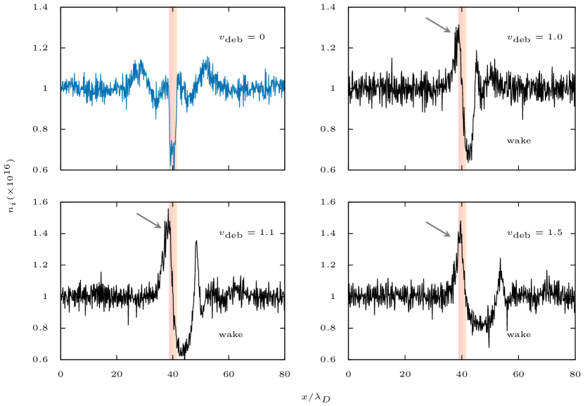
Figure 1: Formation of DSW in ion density due to an negative external charge perturbation. The vertical colored stripe, in each panel, indicates the position of the Gaussian shaped negative charge debris. The arrows indicate the DSW structure as the debris move from right to left with velocity $v_{{\rm deb}}$ (normalized by ion-sound speed $c_{s}$). For a static perturbation, what we see is the propagation of an IAW from the site of initial perturbation, which changes to a DSW as velocity increases.

II.1 Formation of DSW

In this section, we present the results of a 1-D PIC simulation of formation of DSWs, when there is a strong presence of positively charged external Debye-scale structure (the debris). The PIC code used in these simulations is the h-PIC-MCC code, which can simulate plasma processes in the IA, DIA, and electron time scales with dust-charge fluctuation. More about this code and its benchmarking results can be found in the papers by Changmai and Bora [13, 14] and Das et al. [15].

The results of this PIC simulation of this model of an $e$-$i$ plasma are shown in Fig.1 (this study), which shows the formation of DSW when $v_{{\rm deb}}\geq c_{s}$, where $c_{s}=\sqrt{T_{e}/m_{i}}$ is the ion-sound speed with temperature expressed in energy units for $\rho_{{\rm deb}}>0$. The debris is a Gaussian-shaped charge distribution with width $\sim\lambda_{D}$, a few Debye lengths shown as an orange strip in Fig.1. The relevant plasma parameters in this case are as follows: plasma number density $n_{i}\sim n_{e}=10^{16}\,{\rm m}^{-3}$, electron temperature $T_{e}=1\,{\rm eV}$, ion temperature $T_{i}=0.01\,{\rm eV}$, and $|\rho_{{\rm deb}}|\sim 2.5\times 10^{-3}\rho_{0}$, where $\rho_{0}=en_{i,e}$ is the equilibrium plasma density and $e$ being the value of electronic charge. As can be seen from the figure, for a static debris, the perturbation results formation of IAW, which propagates aways from the site of the debris, while a dispersive (oscillating) shock front appears on the front of the debris with an IA wake. These results are broadly in agreement with fluid simulation results, as reported by Sarkar and Bora [5], which also provides a purely theoretical explanation of these oscillations in terms of nonlinear Schrödinger equation (NLSE) in the plasma potential $\phi$ [5].

III Counter-streaming ions

We now focus on the situation what happens, when a Debye-scale structure (debris) of negative charge causes ions to counter-stream and ram into one another, causing an ion-ion two-stream electrostatic instability to develop and become turbulent when the debris charge is considerably large. In what follows, we shall build up a kinetic model for this to happen and follow it up with a PIC simulation.

III.1 Linear theory

Here, we are going to briefly describe the linear theory of electrostatic stability in a plasma with equilibrium velocities in the framework of kinetic theory. Let us consider a multi-species, quasi-neutral, collision-less plasma with different species, having different equilibrium drift velocities. The basic governing equations are the electrostatic Boltzmann-Vlasov equations for different species and Poisson equation for closure

$$\frac{\partial f_{j}}{\partial t}+\bm{u}_{j}\cdot\nabla f_{j}+\frac{q_{j}}{m_{j}}\bm{E}\cdot\frac{\partial f_{j}}{\partial\bm{u}_{j}} = 0,$$ (4)

$$\epsilon_{0}\nabla\cdot\bm{E} = \sum_{j}q_{j}n_{j},$$ (5)

where $(f,\bm{u},q,n)_{j}$ are the velocity distribution function (VDF), velocity, charge, and number density of the $j$th species and $\bm{E}$ is the electric field. The VDF is in general can be expressed as a function of velocities and temperature for each species. For Maxwellian case, it becomes

$$f_{j}(u)\sim\exp\left[-\frac{(u-v_{j})^{2}}{2c_{j}^{2}}\right],$$ (6)

where $v_{j}$ and $c_{j}$ are the equilibrium drift velocity and sound speed of the $j$th species, respectively,

$$c_{j}=(T_{j}/m_{j})^{1/2},$$ (7)

where the temperature is expressed in energy unit with $T_{j}$ and $m_{j}$ being the temperature and particle mass of the $j$th species.

We now introduce a small electrostatic perturbation and express various physical quantities $F$ with a linear perturbation scheme, $F=F_{0}+F_{1}$, where $F_{0,1}$ are equilibrium and perturbed parts. In our case

$$F=(f,\bm{E}),\quad F_{1}\sim e^{-i\omega t+i\bm{k}\cdot\bm{r}},$$ (8)

where the perturbed part is expressed in Fourier harmonics. The first-order Boltzmann-Vlasov equation becomes

$$\frac{\partial f_{j1}}{\partial t}+\bm{u}_{j}\cdot\nabla f_{j1}+\frac{q_{j}}{m_{j}}\bm{E}_{1}\cdot\frac{\partial f_{j0}}{\partial\bm{u}_{j}}=0.$$ (9)

Without loss of any generality, we assume the perturbation to be in $\hat{\bm{x}}$ direction so that the perturbed VDF can be written as

$$f_{j1}=-\frac{iq_{j}}{m_{j}}E_{1x}\left(\frac{\partial f_{j0}/\partial u_{j}}{\omega-ku_{j}}\right),$$ (10)

where $u_{j}\equiv\bm{u}_{j}\cdot\hat{\bm{x}}$. Using the linearised Poisson equation, we finally have

$$\epsilon_{0}\nabla\cdot\bm{E}_{1}=\sum_{j}q_{j}n_{j1},$$ (11)

where $n_{j1}$ is the perturbed number density of the $j$th species, expressed as a fluid quantity, through the perturbed VDF,

$$n_{j1}=\int f_{j1}\,d\bm{u}_{j},$$ (12)

where the integration has to be carried over the 3-dimensional velocity space.

We now write the VDF $f_{j}$ in terms of the unit-normalised VDF $\hat{f}_{j}$, so that

$$f_{j0}\equiv n_{j0}\hat{f}_{j0}.$$ (13)

The one-dimensional normalised VDF for $j$th species can be written as

$$\hat{f}_{j0}(u)=\left(2\pi c_{j}^{2}\right)^{-1/2}\exp\left[-\frac{(u-v_{j})^{2}}{2c_{j}^{2}}\right],\quad\int\hat{f}_{j0}\,d\bm{u}=1.$$ (14)

Substituting all the expressions in the perturbed Poisson equation, Eq.(11), we finally arrive at the linear dispersion equation

$$k^{2}-\sum_{j}\omega_{pj}^{2}\int_{-\infty}^{+\infty}\frac{\hat{f}_{j0}^{\prime}}{u_{j}-\omega/k}\,du_{j}=0,$$ (15)

where $\omega_{pj}$ is the plasma frequency of the $j$th species and

$$\hat{f}_{j0}^{\prime}=\frac{\partial\hat{f}_{j0}}{\partial u_{j}}.$$ (16)

We know that the integral in the above dispersion relation is singular, which leads to the well-known Landau damping term in a plasma with no equilibrium drift velocities. In any case, the singular integral can be evaluated approximately assuming that the singularity lies very close to the real $u$-axis [23]. Decomposing the integral into a non-singular part in terms of Cauchy principal value integration and the approximating singular part through residue theorem, we ,

$$\int_{-\infty}^{+\infty}\frac{\hat{f}_{j0}^{\prime}}{u_{j}-\omega/k}\,du_{j}\simeq\mathbb{P}\int_{-\infty}^{+\infty}\frac{\hat{f}_{j0}^{\prime}}{u_{j}-\omega/k}\,du_{j}+i\pi\left.\hat{f}_{j0}^{\prime}\right|_{u_{j}=\omega/k},$$ (17)

where $\mathbb{P}$ indicates the principal value integration. The final dispersion relation is now given as

$$k^{2}-\sum_{j}\omega_{pj}^{2}\left(\mathbb{P}\int_{-\infty}^{+\infty}\frac{\hat{f}_{j0}^{\prime}}{u_{j}-\omega/k}\,du_{j}+i\pi\left.\hat{f}_{j0}^{\prime}\right|_{u_{j}=\omega/k}\right)=0.$$ (18)

III.2 Counter-streaming ions and electrons

The situation, we are particularly looking at is counter-streaming ions and electrons, which ideally requires four populations of ions and electrons, both counter-streaming in opposite directions. However, in order to simplify the mathematics, we shall consider one drifting population of ions with velocity $v$, while the other population is considered to be static. This can be viewed as considering the situation from the frame of reference of only population of ions. Besides, in order to eliminate kinetic effects of the electrons, we consider electrons to be Boltzmannian. Thus the ion VDFs are given by

$$\hat{f}_{i0}(u)=\frac{1}{\sqrt{2\pi c_{i}^{2}}}\left\{\exp\left[-\frac{u^{2}}{2c_{i}^{2}}\right]+\exp\left[-\frac{(u-v)^{2}}{2c_{i}^{2}}\right]\right\}.$$ (19)

The linearized Poisson equation Eq.(11) becomes

$$ik\epsilon_{0}E_{1x}=-en_{e1}+en_{i1},$$ (20)

with

$$n_{e1} = n_{0}\,\exp\left(\frac{e\phi_{1}}{T_{e}}\right),$$ (21)

$$n_{i1} = \int f_{i1}\,d\bm{u}_{i},$$ (22)

where $f_{i1}$ is given by Eq.(10). Substituting the expressions, we have

$$k^{2}=-\frac{1}{\lambda_{De}^{2}}+\frac{1}{2}\omega_{pi}^{2}\left(\int_{-\infty}^{+\infty}\frac{F^{\prime}(u)}{u-\omega/k}\,du+\int_{-\infty}^{+\infty}\frac{F^{\prime}(\tilde{u})}{u-\omega/k}\,du\right),$$ (23)

where we have substituted $\phi_{1}=iE_{1x}/k$ and

$$F(u)=\frac{1}{\sqrt{2\pi c_{i}^{2}}}\exp\left(-\frac{u^{2}}{2c_{i}^{2}}\right),$$ (24)

with $\tilde{u}=u-v$. Note that each ion population is responsible for half of the total ion density. Expressing $u$ in terms of $\tilde{u}$, the second integration can be written as

$$\int_{-\infty}^{+\infty}\frac{F^{\prime}(\tilde{u})}{\tilde{u}-\tilde{\omega}/k}\,d\tilde{u},$$ (25)

where $\tilde{\omega}=\omega-kv$ is the Doppler-shifted frequency. For small $\textrm{Im}(u,\tilde{u})$, one can approximate Eq.(23) as

$$k^{2} = -\frac{1}{\lambda_{De}^{2}}+\frac{1}{2}\omega_{pi}^{2}\left(\mathbb{P}\int_{-\infty}^{+\infty}\frac{F^{\prime}(u)}{u-\omega/k}\,du+\mathbb{P}\int_{-\infty}^{+\infty}\frac{F^{\prime}(u)}{u-\tilde{\omega}/k}\,du\right)$$ (26)

$$+\,i\pi\frac{1}{2}\omega_{pi}^{2}\left(\left.\frac{\partial F}{\partial u}\right|_{u=\omega/k}+\left.\frac{\partial F}{\partial u}\right|_{u=\tilde{\omega}/k}\right).$$

The principal value integrations can be found out to be

$$\mathbb{P}\int_{-\infty}^{+\infty}\frac{F^{\prime}(u)}{u-\omega/k}\,du \simeq \frac{k^{2}}{\omega^{2}}\left\langle(1-ku/\omega)^{-2}\right\rangle,$$ (27)

$$\mathbb{P}\int_{-\infty}^{+\infty}\frac{F^{\prime}(u)}{u-\tilde{\omega}/k}\,du \simeq \frac{k^{2}}{(\omega-kv)^{2}}\left\langle(1-ku/\tilde{\omega})^{-2}\right\rangle,$$ (28)

where $v_{\phi}=\omega/k$ and $\tilde{v}_{\phi}=\tilde{\omega}/k$ the phase velocities. The angular brackets indicate average of the quantity with respect to the equilibrium VDFs $F(u)$ and $F(\tilde{u})$, respectively. The quantities inside the $\left\langle\right\rangle$ provide the correction terms to the ion-plasma oscillation frequency and to the first order, can be neglected if we ignore its effect on counter-streaming instability. Approximating $\left\langle\right\rangle\sim 1$, we have

$$\omega^{2}\left(1+\frac{1}{k^{2}\lambda_{De}^{2}}\right)-i\pi\frac{1}{2k^{2}}\omega^{2}\omega_{pi}^{2}\left(\left.\frac{\partial F}{\partial u}\right|_{u=\omega/k}+\left.\frac{\partial F}{\partial u}\right|_{u=\tilde{\omega}/k}\right)\simeq\frac{1}{2}\omega_{pi}^{2}\left[1+\frac{\omega^{2}}{(\omega-kv)^{2}}\right].$$ (29)

Approximating $\omega\sim\omega_{pi}$ on the right hand side, we can simplify the above equations as

$$\omega^{2}\simeq\frac{1}{2}\alpha\omega_{pi}^{2}\left(1+\tilde{\omega}_{pi}^{2}\right)\left[1-i\pi\alpha\frac{\omega_{pi}^{2}}{2k^{2}}\left(\left.\frac{\partial F}{\partial u}\right|_{u=\omega/k}+\left.\frac{\partial F}{\partial u}\right|_{u=\tilde{\omega}/k}\right)\right]^{-1},$$ (30)

where

$$\alpha = \left(1+\frac{1}{k^{2}\lambda_{De}^{2}}\right)^{-1},$$ (31)

$$\tilde{\omega}_{pi} = \frac{\omega_{pi}^{2}}{(\omega_{pi}-kv)^{2}}.$$ (32)

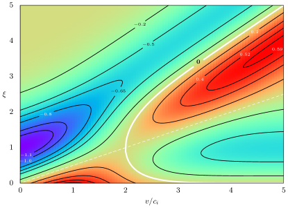
Figure 2: Contour plot of the function ${\cal F}$.

For small $\textrm{Im}(\omega)$, one can expand the above expression to get an expression for the growth rate as

$$\textrm{Im}(\omega)\simeq\pi\left(\frac{\alpha}{2}\right)^{3/2}\frac{\omega_{pi}^{3}}{2k^{2}}\left(1+\tilde{\omega}_{pi}^{2}\right)^{1/2}\left(\left.\frac{\partial F}{\partial u}\right|_{u=\omega/k}+\left.\frac{\partial F}{\partial u}\right|_{u=\tilde{\omega}/k}\right).$$ (33)

We note that

$$\left.\frac{\partial F}{\partial u}\right|_{u=\omega/k} = -\frac{\omega}{kc_{i}^{3}\sqrt{2\pi}}\exp\left[-\frac{(\omega/k)^{2}}{2c_{i}^{2}}\right],$$ (34)

$$\left.\frac{\partial F}{\partial u}\right|_{u=\tilde{\omega}/k} = -\frac{(\omega/k-v)}{c_{i}^{3}\sqrt{2\pi}}\exp\left[-\frac{(\omega/k-v)^{2}}{2c_{i}^{2}}\right],$$ (35)

so that the growth rate of the instability can be approximated as

$$\textrm{Im}\left(\frac{\omega}{\omega_{pi}}\right)\simeq\frac{1}{8}\sqrt{\alpha^{3}\pi}\left(\frac{\omega_{pi}}{kc_{i}}\right)^{3}\left(1+\tilde{\omega}_{pi}^{2}\right)^{1/2}\left\{\left(\frac{kv}{\omega_{pi}}-1\right)\exp\left[-\frac{(\omega_{pi}-kv)^{2}}{2k^{2}c_{i}^{2}}\right]-\exp\left[-\frac{\omega_{pi}{}^{2}}{2k^{2}c_{i}^{2}}\right]\right\}$$ (36)

where we have set $\omega\sim\omega_{pi}$ on the right hand side.

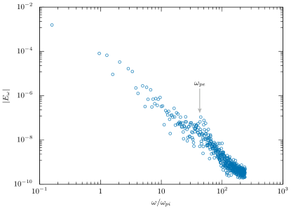
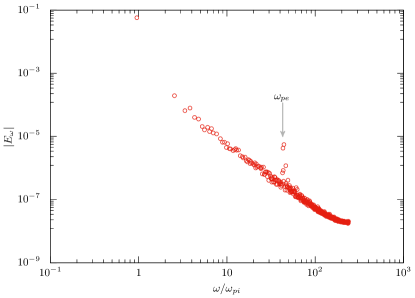
Figure 3: The power spectrum density (PSD) for random fluctuations (left) and a fully developed turbulence (right).

III.3 Critical velocity

Normalizing $v\to v/c_{i}$ and $\gamma=\textrm{Im}(\omega/\omega_{pi})$, one can conveniently express the above expression as

$$\gamma=\frac{1}{8}\xi^{2}\sqrt{\pi\alpha^{3}}\left(1+\tilde{\omega}_{pi}^{2}\right)^{1/2}{\cal F},$$ (37)

where

$${\cal F}=\left(v-\xi\right)\exp\left[-\frac{(v-\xi)^{2}}{2}\right]-\xi\exp\left(-\frac{\xi^{2}}{2}\right).$$ (38)

with $\xi=1/(k\lambda_{Di})$ and $\gamma$ as the normalized growth rate, the sign of which is determined by ${\cal F}$. A contour plot of the term ${\cal F}$ is shown in Fig.2. As represented in the figure, one can find out the minimum critical velocity $v_{c}$ required to excite the instability $(\gamma>0)$ can be calculated from the curve ${\cal F}=0$ by seeking the minimum $v$. However, solutions of the equation ${\cal F}=0$ can only be expressed in terms inverse functions and in general one cannot obtain a full spectrum of solutions including the equation for the curve of minimum $v$ (the white curve in Fig.2). One can however obtain $v_{c}$ by expanding ${\cal F}$ around $\xi=1$ and find the solution of the resultant equation after setting $dv/d\xi=0$ as,

$$(v_{c}-2)\exp\left[-\frac{(v-1)^{2}}{2}\right]=0,$$ (39)

which yields $v_{c}=2$. In terms of plasma sound speed $c_{s}=\sqrt{T_{e}/m_{i}}$, $v_{c}\simeq 2\sqrt{\sigma}c_{s}$ and $\sim 0.63c_{s}$ for $\sigma=0.1$, which is quite within the limit $c_{s}>v_{{\rm deb}}>1.3c_{i}$ [18]. For a situation when external charge perturbation (i.e. debris) is stationary relative to the plasma, it is the debris potential which causes acceleration of the ion. The maximum velocity $v_{\textrm{max}}$ an ion can obtain for a potential difference of $\varphi$ between the debris and bulk plasma can be found by equating the electrostatic energy to the kinetic energy of the ions $v_{\textrm{max}}=(2ef\varphi/m_{i})^{1/2}$, where $f$ is the fraction of electrostatic energy that is converted to kinetic energy of the ions, which lies between $0$ and $1$ and $e$ is the electronic charge. Normalizing the potential by $(T_{e}/e)$ and velocity by $c_{s}$, we find $\phi=v_{\textrm{max}}^{2}/(2f)\sim 2\sigma f^{-1}$. Usually, when we consider the acceleration of charged particles through an electrostatic potential drop, we consider the source of the potential to be infinitely large so that all particles get accelerated equally. However, in this case when an ion is accelerated by the debris potential, it will reduce the potential for the subsequent particles and the effective potential available for incoming particles will be continuously reduced, which is being taken care of by the factor $f$, much like Debye shielding.

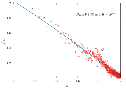
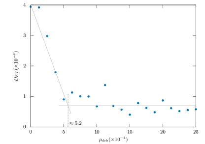
Figure 4: The divergence $D_{KL}(P\parallel Q)$ for random fluctuation is shown in the left panel. Note that both the axes are normalized to the interval $[1,2]$. A plot of $D_{KL}(P\parallel Q)$ versus external charge density $\rho_{\textrm{deb}}$ normalized to equilibrium charge density is shown in the right panel. The sudden change of behaviour of $D_{KL}(P\parallel Q)$ signify the onset of turbulence.

IV Onset of turbulence

We shall now try to see the onset of the turbulence due to external charge perturbation or debris. Computationally, in order to quantify the onset of turbulence, we plot the power spectrum density (PSD) $|E_{\omega}|$ of the kinetic energy against frequency $\omega$. The results are shown in Fig.3.

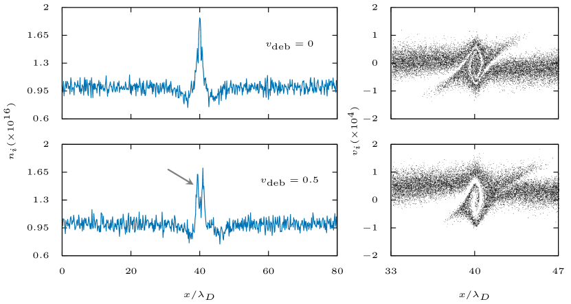
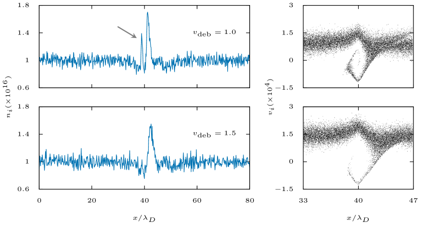
Figure 5: Formation of pinned solitons at the debris site as the debris velocity $v_{{\rm deb}}$ (measured in terms of $c_{s}$) exceeds a certain value. In the figure, we have shown the ion density $n_{i}$ (left panel) and the corresponding phase-space for the pinned solitons, showing phase-space vortices, indicating electrostatic turbulence. The arrow shows the pinned soliton. Pinned soliton ceases to form at higher $v_{{\rm deb}}$ (lower panels).

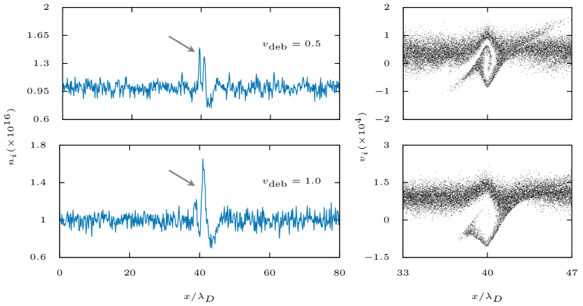
Figure 6: Effect of negatively charged dust particles on amplitude of pinned solitons, corresponding to the same cases for $v_{{\rm deb}}=0.5,1.0$ without any dust (see corresponding panels in Fig.5). The reduced amplitude of pinned solitons is clearly visible.

In the figure, we have shown the PSDs – one for random fluctuation in the plasma when no particular perturbation is present (left panel) and one when an external negative charge perturbation is introduced, resulting a fully developed turbulence (right panel). As is evident from the figure, we can clearly see a Kolmogorv-type scaling in the right panel, signifying turbulence. The relevant parameters for an 1-D plasma are as follows: the equilibrium plasma density $n_{0}\sim 10^{16}\,\textrm{m}^{-1}$ and electron temperature $T_{e}\sim 1\,\textrm{eV}$ with $\sigma=0.01$. Assuming that a fully developed turbulence results in a Kolmogorv-type inverse-cascading scaling, we try to detect the onset of turbulence by looking at the deviation of the PSD from that of Kolmogorv-type scaling, when strength of the external charge debris exceeds a certain threshold. In order to carry out the computational analysis, we estimate the so-called divergence of a dataset for PSD from the ideal one (Kolmogorov-type) by calculating the relative entropy, also known as Kullback–Leibler divergence, denoted as $D_{KL}(P\parallel Q)$. This method treats the datasets as distributions $P$ (ideal Kolmogorov-type distribution) and $Q$ (PSD distribution obtained from simulation) and estimate the divergence of the target distribution $Q$ from the sample distribution $P$. The lower is the value of the divergence, the more closer is the distribution $Q$ to $P$. To start with, we generate the ideal Kolmogorov-type distribution $P$ by fitting the following nonlinear function to the distribution $Q$,

$$P\equiv\hat{f}_{\textrm{PSD}}=a+bp^{c},$$ (40)

in the $\log$-$\log$ space. In the above fitting $p$ denotes a point on the PSD spectrum and $a,b,c$ are fitting constants. This fitting is inspired by the Kolmogorov-type inverse-cascading power law. It is to be noted that in order to avoid complex singularity in the dataset, we have normalized the target dataset to a positive definite interval of $[1,2]$ on both axes, although in principle one can normalize it to any arbitrary interval. The results of the analysis is summarized through Fig.4, where we have shown the calculation of this divergence for random fluctuation (left), for which which is $D_{KL}(P\parallel Q)\simeq 4.48\times 10^{-4}$. On the right panel, we have plotted the divergence $D_{KL}(P\parallel Q)$ for various debris charge $\rho_{\textrm{deb}}$ (external perturbation). From the figure, what we see is a sudden shift in the value of the divergence from a linear decrease to a near-constant state, signifying the onset of turbulence. The point of onset can be found from the intersection of the two curves as shown in the figure, which comes out to be $\rho_{\textrm{deb}}\sim 5.2\times 10^{-4}$, normalized to the equilibrium charge density which is unity.

It is also interesting to see the scaling law of this turbulence, which is shown in Fig.7. The energy-wave number scaling $E_{k}\propto k^{-\kappa}$ ranges from a very steep slope with $\kappa\sim 5.64$ to about $\kappa\sim 1.92$. Note that a typical Kolmogorv-type scaling is $5/3\,(\simeq 1.67)$.

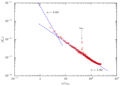
Figure 7: Kolmogorv-type power laws $(E_{k}\propto k^{-\kappa})$ for the ion-ion counter-streaming electrostatic turbulence.

IV.1 Pinned solitons

We have seen how an external, charged debris can excite counter-streaming ion instability, which results in an electrostatic turbulence as debris charge density exceeds a certain value. In what follows, we shall see how this electrostatic turbulence gives rise to pinned solitons as velocity of the debris exceeds certain value. From the simulation, it is amply apparent that the ion phase-space vortices, resulting out of the electrostatic turbulence, can trap the ions which causes pinned solitons to form. As the simulation progresses, we expect to see more number of vortices which may lead to more number of pinned solitons being formed.

The results of this simulation are shown in Fig.5, in which we plot the ion density $n_{i}$ as well as the scatter plot of the ion phase-space for various $v_{{\rm deb}}$. We see that as debris velocity increases, it causes widening of the vortices causing well-separated pinned solitons. In the limit of $v_{{\rm deb}}\to 0$, the single soliton that we can see is nothing but the merger of multiple pinned solitons. However, when $v_{{\rm deb}}\gg c_{s}$, the vortices are widened up to a limit where pinned solitons cannot form. So, pinned solitons can form only within an window of debris velocity. These results are consistent with the findings of Tiwari [1] and Sarkar [5].

IV.2 Dust effects

As shown in many other works [5], presence of negatively charged dust particles increases the effective ion-sound speed of plasma making near-sonic events sub-sonic. In the limit of large wavelength perturbation $(k\lambda_{D}\gg 1)$ and negligible ion temperature $(\sigma\ll 1)$, the IA dispersion relation becomes [5]

$$\omega\simeq k\left(\frac{n_{i0}}{n_{e0}}\right)^{1/2}c_{s}.$$ (41)

Note that in presence of negative dust particles $n_{i0}/n_{e0}>1$ due to depletion of electrons, the overall effect can be viewed as an effective increase of sound speed $c_{{\rm effective}}$, with

$$c_{{\rm effective}}=\left(\frac{n_{i0}}{n_{e0}}\right)^{1/2}c_{s}.$$ (42)

This effect can be clearly seen in Fig.6, where we have included negatively charged dust particles. The dust particles are assumed to be cold the number density is assumed to be constant at $10^{15}\,{\rm m}^{-3}$. The h-PIC-MCC code consistently takes the dust-charging as well as dust-charge fluctuation into account [14, 15]. In Fig.6, one can directly compare the corresponding results for zero-dust cases in Fig.5 (second and third panels from top) where we see the reductions of amplitudes of pinned solitons for $v_{{\rm deb}}=0.5$ and $1.0$.

V Summary and conclusions

In summary, we in this work, have considered an $e$-$i$ plasma in the presence of an external, gaussian-shaped charge perturbation (debris) moving through the plasma in an ion-acoustic time scale. It is now well-known that the response of the plasma differs significantly depending on the nature and the magnitude of debris charge density and its velocity [5], which is now being re-confirmed for the first time with an 1D PIC simulation. The simulation is being carried out with the well-tested h-PIC-MCC code [13, 14, 15], which can take into account dust and dust-charge fluctuation self-consistently. We have shown that while a positively charged external perturbation produces a DSW in the precursor region, a negatively charged perturbation causes ion-ion counter-streaming instability, which quickly become turbulent giving rise to the pinned solitons when debris velocity becomes near sonic and supersonic. These pinned solitons however dies down when debris velocity becomes highly supersonic. In the ion density plot as well as in the scatter plot of the ion phase-space for various debris velocity, we see that when debris velocity increases, it causes widening of the vortices causing well-separated pinned solitons, which merges to form one single soliton when debros velocity reduces to zero. In the opposite extreme, when debris velocity becomes too large, it widens the vortices causing the pinned solitons to disappear.

Through this work, we have shown, for the first time, that the pinned solitons are actually manifestation of the ion phase-space vortices formed in the turbulent regime of the ion-ion counter-streaming kinetic instability, where ions are effectively trapped in the potential structure. Our simulation results are supported by the linear kinetic theory, through which we have shown the existence of critical debris charge density for the instability to turn turbulent. We have shown that a $E_{k}\propto k^{-\kappa}$, Kolmogorv-type inverse-cascading of exists in the turbulent regime which support the pinned solitons.

Toward the end, we have shown the effect of negatively charged dust particles on the pinned solitons, which causes the amplitude of the solitons to decrease and require relatively large debris velocity to make the pinned solitons appear as compared to the case when there is no dust particles. These results largely agree with the fluid simulation results [5].

References

- [1] S. K. Tiwari and A. Sen, Phys. Plasmas 23, 022301 (2016).
- [2] A. Sen, S. Tiwari, S. Mishra, and P. Kaw, Adv. Space Res. 56, 429 (2015).
- [3] S. K. Tiwari and A. Sen, Phys. Plasmas 23, 100705 (2016).
- [4] A. Kumar and A. Sen, New J. Phys. 22, 073057 (2020).
- [5] H. Sarkar and M. P. Bora, Phys. Plasmas 30, 083701 (2023).
- [6] G. Arora, P. Bandyopadhyay, M. G. Hariprasad, and A. Sen, Phys. Rev. E 103 (2021).
- [7] S. Jaiswal, P. Bandyopadhyay, and A. Sen, Phys. Rev. E 93, 041201(R) (2016).
- [8] G. Arora, P. Bandyopadhyay, M. G. Hariprasad, and A. Sen, Phys. Plasmas 26 (2019).
- [9] R. W. et al., Astrophys. J. Lett. 889:L9 (2020).
- [10] M. Khusroo and M. P. Bora, Phys. Rev. E 99, 013205 (2019).
- [11] I. Y. Vasko, F. S. Mozer, and V. V. e. a. Krasnoselskikh, Gephys. Res. Lett. 45, 5809 (2018).
- [12] J. L. Burch, T. E. Moore, R. B. Torbert, and B. L. Giles, Space Sci. Rev. 199, 5 (2016).
- [13] S. Changmai and M. P. Bora, Phys. Plasmas 26 (2019).
- [14] S. Changmai and M. P. Bora, Sci. Rep. 10, 20980 (2020).
- [15] M. Das, S. Changmai, and M. P. Bora, Phys. Rev. E 108, 045202 (2023).
- [16] J. D. Jackson, J. Nucl. Energy, Part C Plasma Phys. 1, 171 (1960).
- [17] D. W. Forslund and C. R. Shonk, Phys. Rev. Lett. 25, 281 (1970).
- [18] T. E. Stringer, J. Nucl. Energy, Part C Plasma Phys. 6, 267 (1964).
- [19] D. V. Rose, T. C. Genoni, D. R. Welch, E. A. Startsev, and R. C. Davidson, Phys. Rev. ST Accel. Beams 10 (2007).
- [20] M. E. Dieckmann, L. O. Drury, and P. K. Shukla, New J. Phys. 8, 40 (2006).
- [21] D. F. Smith and P. C. W. Fung, J. Plasma Phys. 5, 1 (1971).
- [22] Y. Kiwamoto, J. Phys. Soc. Jpn. 37, 466 (1974).
- [23] F. F. Chen, Introduction to plasma physics and controlled fusion, volume 1, Plenum Press, New York and London, second edition, 1974.