Uncovering the Higher-Order Structure of Social Systems

A Higher-Order Lens for Social Systems

Despite the widespread adoption of higher-order mathematical structures such as hypergraphs, methodological tools for their analysis lag behind those for traditional graphs. This work addresses a critical gap in this context by proposing two micro-canonical random null models for directed hypergraphs: the Directed Hypergraph Configuration Model (DHCM) and the Directed Hypergraph JOINT Model (DHJM). These models preserve essential structural properties of directed hypergraphs such as node in- and out-degree sequences and hyperedge head and tail size sequences, or their joint tensor. We also describe two efficient MCMC algorithms, NuDHy-Degs and NuDHy-JOINT, to sample random hypergraphs from these ensembles.

To showcase the interdisciplinary applicability of the proposed null models, we present three distinct use cases in sociology, epidemiology, and economics. First, we reveal the oscillatory behavior of increased homophily in opposition parties in the US Congress over a 40-year span, emphasizing the role of higher-order structures in quantifying political group homophily. Second, we investigate non-linear contagion in contact hyper-networks, demonstrating that disparities between simulations and theoretical predictions can be explained by considering higher-order joint degree distributions. Last, we examine the economic complexity of countries in the global trade network, showing that local network properties preserved by NuDHy explain the main structural economic complexity indexes.

This work pioneers the development of null models for directed hypergraphs, addressing the intricate challenges posed by their complex entity relations, and providing a versatile suite of tools for researchers across various domains.

1 Introduction

Higher-order mathematical structures such as hypergraphs and simplicial complexes have emerged as powerful modeling tools that overcome the limitations of traditional graph models, which by construction are restricted to binary relations between entities  (?, ?, ?). Indeed, their adoption is motivated by the observation that real-world scenarios often entail interactions among multiple entities simultaneously. Examples span systems across multiple spatial and temporal scales, including cellular processes  (?), protein interaction networks  (?), neural processing  (?, ?), whole-brain activity  (?, ?), co-authorship networks  (?, ?), and contact networks  (?). Hypergraphs, in particular, are a natural and flexible generalization of graphs that model arbitrary $q$-ary relations among entities. Directed hypergraphs further extend this concept by representing a link from a set of nodes (the head of the hyperedge) to another set of nodes (its tail). Consider, for instance, the case of citations among scientific publications. In this case, each citation in a publication can be modeled as a directed hyperedge from the set of authors of the publication to the set of authors of the cited work. The application of hypergraphs already spans diverse domains, from forecasting urban traffic  (?) and modeling Bitcoin transactions  (?) to representing web structures for accurate page reputation scoring  (?). However, the current methodological tools for hypergraphs lag behind their counterparts in the graph world.

Understanding complex networks often involves comparing observed structures against models that mimic random scenarios. Originating from Fisher’s groundwork in hypothesis testing  (?), this methodology has expanded into graph theory with the study of random graph null models  (?). These models define graph ensembles that retain only selected features of the observed graph while being random in any other respect  (?). They are key tools in graph theory because they allow us to assess the significance of the observed properties of real-world networks, by comparing them to those obtained from randomly generated graphs  (?). This comparative analysis unveils the influence of local node features versus additional factors on network properties, and aids in identifying structural irregularities within the networks (?). Furthermore, it enables assessing the role of specific properties in the presence of specific empirically-observed topological and structural features.

Akin to any hypothesis test, the selection of topological features to preserve in these ensembles significantly influences the conclusions drawn from the analyses. Common approaches preserve the degree sequence  (?, ?) and the joint degree sequence  (?, ?). Random graph ensembles can be categorized into two fundamental families: micro-canonical and canonical  (?). Micro-canonical ensembles preserve the properties in a ‘hard’ fashion, i.e., each of the graphs in the ensemble satisfies the imposed constraints. Conversely, canonical ensembles preserve the properties in a ‘soft’ fashion: they maintain the constraints in expectation across the graphs in the ensemble. The choice between these approaches should be based on principled criteria, considering factors such as the characteristics of the observed data. Canonical ensembles, for instance, are better suited for scenarios where data may contain measurement errors or noise since they maintain constraints on an average basis.

Despite a vast literature on canonical and micro-canonical graph ensembles  (?, ?, ?, ?, ?, ?, ?, ?), little attention has been devoted to defining null models for directed hypergraphs and developing efficient sampling algorithms for their corresponding ensembles. Existing work in the realm of hypergraphs predominantly focuses on configuration models for undirected hypergraphs  (?, ?, ?, ?, ?, ?, ?), introduces max entropy models  (?), or generalizes the concept of dK-series to undirected hypergraphs  (?, ?).

Transitioning to developing null models for directed hypergraphs brings unique challenges due to their intricate entity relations, characterized by a broader set of properties—and thus constraints. Parameters such as the number of nodes, number of hyperedges, head and tail size sequences, and the frequency of nodes within hyperedge heads or tails should be taken into consideration when defining these models. Recently, Kim et al.  (?) proposed two samplers for generating directed hypergraphs in the canonical ensemble with prescribed head and tail size sequences. However, due to certain design choices aimed at improving efficiency, the generated hypergraphs often exhibit structural dissimilarities from the real-world ones.

This work proposes two micro-canonical null models for directed hypergraphs. The first model, Directed Hypergraph Configuration Model (DHCM), preserves the in- and out-degree sequences of the nodes, as well as the head-size and tail-size sequences of the hyperedges. The second model, called Directed Hypergraph JOINT Model (DHJM), preserves the joint out-in degree tensor, which encodes information about the in- and out-degree of the nodes involved in hyperedges of specific head and tail sizes. We also describe two samplers, NuDHy-Degs and NuDHy-JOINT, to efficiently draw random hypergraphs from the corresponding ensembles. Both samplers are Markov Chain Monte Carlo algorithms based on Metropolis-Hastings and employ targeted shuffling operations for traversal within the Markov graph.

We demonstrate the wide interdisciplinary applicability of the proposed suite of null models by showcasing three distinct use cases in sociology, epidemiology, and economics, respectively. The first one shows the role of higher-order structures in quantifying genuine political group homophily by uncovering an oscillatory behavior of increased homophily in opposition parties in the US Congress across a 40-years span. The second one focuses on nonlinear contagion in contact hyper-networks, demonstrating that the disparities observed between simulations in the hyper-networks and theoretical predictions can be explained when considering higher-order joint degree distribution, thus shedding some light on the underlying mechanisms governing these phenomena. The third and final one studies the economic complexity of countries in the global trade network, and shows that the main structural economic complexity indexes  (?, ?, ?) can be almost entirely explained by local properties of the network preserved by NuDHy. A more comprehensive evaluation of NuDHy with respect to other existing null models and related samplers is provided in Appendix G.

2 Null Models for Weighted Directed Hypergraphs

We consider weighted directed hypergraphs of the form $H\doteq(V,E)$, where $V=\{v_{1},\ldots,v_{n}\}$ is a set of nodes and $E=\{e_{1},\ldots,e_{m}\}$ is a multi-set of directed hyperedges where the multiplicity of each hyperedge represents its weight. Each hyperedge $e\doteq(h,t)\in E$ consists of a head $h$ and a tail $t$ such that $h,t\subseteq V$. The size of $e$ is the sum of the sizes of its head and tail, $\left\lvert{e}\right\rvert=\left\lvert{h}\right\rvert+\left\lvert{t}\right\rvert$. The in-degree of a node $v$ in $H$, denoted as $\mathsf{ideg}_{H}(v)$, is the number of tails that contain $v$; the out-degree of $v$ in $H$, denoted as $\mathsf{odeg}_{H}(v)$, is the number of heads that contain $v$.

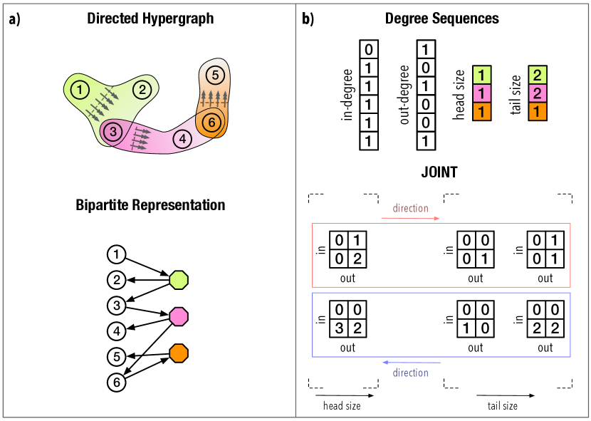
Figure 1: Construction of directed hypergraph configuration models. a) A directed hypergraph (top) and its representation as a bipartite graph (bottom). The left vertices (circles) correspond to hypergraph nodes, while the right vertices (hexagons) correspond to hyperedges. Dotted lines in the directed hypergraph separate the head and tail of each hyperedge, with arrows pointing towards the tail. b) The characteristics of the observed hypergraph preserved by DHCM and DHJM: left and right in- and out-degree sequences (top), and JOINT (bottom). The right in-degree sequence corresponds to the head-size sequence, while the right out-degree sequence corresponds to the tail-size sequence.

A weighted directed hypergraph $H$ can be represented, without loss of information, as a directed bipartite graph $G\doteq(L,R,D)$, where $L=V$ (left vertices), $R=E$ (right vertices), and $D$ is a set of triplets defined as follows:

$$\forall e\doteq(h,t)\in E,\forall v\in h\implies(v,e,+1)\in D;$$

$$\forall e\doteq(h,t)\in E,\forall v\in t\implies(v,e,-1)\in D.$$

Each triplet $(v,e,d)$ is a directed edge involving a node $v$ and a hyperedge $e$, where $d$ denotes the direction of the edge: $+1$ indicates that the edge goes from a left vertex to a right vertex whereas $-1$ indicates the opposite direction. We denote with $\overrightarrow{D}$ the set of pairs of vertices connected by an edge with direction $d=+1$, i.e., $(v,\alpha)\in\overrightarrow{D}\iff(v,\alpha,+1)\in D$. Similarly, we denote with $\overleftarrow{D}$ the set of pairs of vertices connected by an edge with opposite direction $d=-1$. For any vertex $v\in L$, we denote with $\overrightarrow{\Gamma_{G}}(v)$ the set of vertices $\alpha\in R$ such that $(v,\alpha)\in\overrightarrow{D}$, and with $\overleftarrow{\Gamma_{G}}(v)$ the set of vertices $\alpha\in R$ such that $(v,\alpha)\in\overleftarrow{D}$. The size of $\overrightarrow{\Gamma_{G}}(v)$ is called the out-degree of $v$, while the size of $\overleftarrow{\Gamma_{G}}(v)$ is the in-degree of $v$. Similarly, we can define the in-degree (resp. out-degree) of a vertex $\alpha\in R$ as the size of the set of vertices $v\in L$ such that $(v,\alpha)\in\overleftarrow{D}$ (resp. $(v,\alpha)\in\overrightarrow{D}$). Figure 1a shows an example of a directed hypergraph and the corresponding bipartite graph.

To encode the information of both the in- and out-degree of the vertices connected by the edges in $G$, we define the bipartite Joint Out-In degree Tensor (JOINT) $\mathsf{T}_{G}$.

Definition 1 (JOINT).

Let $G\doteq(L,R,D)$ be a directed bipartite graph, and $\mathsf{IN}_{L}=\max\limits_{v\in L}{\left\lvert{\overleftarrow{\Gamma_{G}}(v)}\right\rvert}$ and $\mathsf{OUT}_{L}=\max\limits_{v\in L}{\left\lvert{\overrightarrow{\Gamma_{G}}(v)}\right\rvert}$ be the largest in-/out-degree of a vertex in $L$, respectively. $\mathsf{IN}_{R}$ and $\mathsf{OUT}_{R}$ are similarly defined for $R$. The bipartite Joint Out-In degree Tensor (JOINT) $\mathsf{T}_{G}$ of $G$ is a 5-dimensional tensor with size $\mathsf{IN}_{L}+1\times\mathsf{OUT}_{L}+1\times\mathsf{IN}_{R}+1\times\mathsf{OUT}_{R}+1\times 2$, and whose $(i,j,k,l,d)$-th entry $\mathsf{T}_{G}[i,j,k,l,d]$ for $i\in\left[0,\mathsf{IN}_{L}\right]$, $j\in\left[0,\mathsf{OUT}_{L}\right]$, $k\in\left[0,\mathsf{IN}_{R}\right]$, $l\in\left[0,\mathsf{OUT}_{R}\right]$, and $d\in\{+1,-1\}$, is the number of edges with direction $d$ connecting a left vertex with in-degree $i$ and out-degree $j$ and a right vertex with in-degree $k$ and out-degree $l$, i.e.,

$$\mathsf{T}_{G}[i,j,k,l,d]\doteq\left\lvert{\left\{(v,\alpha,d)\in D\mathrel{:}\left\lvert{\overleftarrow{\Gamma_{G}}(v)}\right\rvert=i\wedge\left\lvert{\overrightarrow{\Gamma_{G}}(v)}\right\rvert=j\wedge\left\lvert{\overrightarrow{\Gamma_{G}}(\alpha)}\right\rvert=k\wedge\left\lvert{\overleftarrow{\Gamma_{G}}(\alpha)}\right\rvert=l\right\}}\right\rvert.$$

Null model. Let $\mathcal{P}$ be a set of properties of an observed hypergraph $\mathring{H}$. A null model $\Pi\doteq(\mathcal{Z},\pi)$ is a tuple where $\mathcal{Z}$ is the set of all the hypergraphs where each $P$ in $\mathcal{P}$ holds (i.e., the ensemble of hypergraphs that preserve these properties), and $\pi$ is a probability distribution over $\mathcal{Z}$.

The first null model proposed, called Directed Hypergraph Configuration Model (DHCM) and denoted as $\Pi^{\textsc{DHCM}}\doteq(\mathcal{Z}^{\textsc{DHCM}},\pi)$, preserves the following four properties:

• head-size sequence $\left[|h_{1}|,\dotsc,|h_{m}|\right]$;

• tail-size sequence $\left[|t_{1}|,\dotsc,|t_{m}|\right]$;

• in-degree sequence $\left[\mathsf{ideg}_{\mathring{H}}(v_{1}),\dotsc,\mathsf{ideg}_{\mathring{H}}(v_{n})\right]$;

• out-degree sequence $\left[\mathsf{odeg}_{\mathring{H}}(v_{1}),\dotsc,\mathsf{odeg}_{\mathring{H}}(v_{n})\right]$.

Each $H\in\mathcal{Z}^{\textsc{DHCM}}$ has the same head-size, tail-size, in-degree, and out-degree sequences of $\mathring{H}$. Preserving P1 and P2 is equivalent to preserving the sequences of the out- and in-degrees of the vertices in $R$ in the bipartite graph representation $\mathring{G}$ of $\mathring{H}$, and automatically preserves the sequence of the sizes of the hyperedges in $\mathring{H}$. Preserving P3 and P4 corresponds to preserving the sequences of the in- and out-degrees of the vertices in $L$ in $\mathring{G}$, and automatically preserves the number of times each node is contained in a tail and a head of a hyperedge in $\mathring{H}$. The in-degree, out-degree, head-size, and tail-size sequences of the directed hypergraph in Figure 1a are illustrated in Figure 1b.

The second null model proposed, called Directed Hypergraph JOINT Model (DHJM) and denoted as $\Pi^{\textsc{DHJM}}\doteq(\mathcal{Z}^{\textsc{DHJM}},\pi)$, preserves the following property:

• JOINT $\mathsf{T}_{\mathring{G}}$.

Preserving P5 also preserves P1-P4.

In fact, for every $\bar{a}\in\left[0,\mathsf{IN}_{R}\right]$, $\bar{b}\in\left[0,\mathsf{OUT}_{R}\right]$, $\bar{c}\in\left[0,\mathsf{IN}_{L}\right]$, $\bar{d}\in\left[0,\mathsf{OUT}_{L}\right]$, it holds

$$\text{{P5} preserves {P1}:}\quad\left\lvert{\left\{\alpha\in R\mathrel{:}\mathsf{ideg}_{\mathring{H}}(\alpha)=\bar{a}\right\}}\right\rvert=\nicefrac{{1}}{{\bar{a}}}\sum_{i=0}^{\phantom{.}\mathsf{IN}_{L}\phantom{.}}\sum_{j=0}^{\mathsf{OUT}_{L}}\sum_{l=0}^{\mathsf{OUT}_{R}}\mathsf{T}_{\mathring{G}}[i,j,\bar{a},l,+1]$$

$$\text{{P5} preserves {P2}:}\quad\left\lvert{\left\{\alpha\in R\mathrel{:}\mathsf{odeg}_{\mathring{H}}(\alpha)=\bar{b}\right\}}\right\rvert=\nicefrac{{1}}{{\bar{b}}}\sum_{i=0}^{\phantom{.}\mathsf{IN}_{L}\phantom{.}}\sum_{j=0}^{\mathsf{OUT}_{L}}\sum_{k=0}^{\phantom{.}\mathsf{IN}_{R}\phantom{.}}\mathsf{T}_{\mathring{G}}[i,j,k,\bar{b},-1]$$

$$\text{{P5} preserves {P3}:}\quad\left\lvert{\left\{v\in L\mathrel{:}\mathsf{ideg}_{\mathring{H}}(v)=\bar{c}\right\}}\right\rvert=\nicefrac{{1}}{{\bar{c}}}\sum_{j=0}^{\mathsf{OUT}_{L}}\sum_{k=0}^{\phantom{.}\mathsf{IN}_{R}\phantom{.}}\sum_{l=0}^{\mathsf{OUT}_{R}}\mathsf{T}_{\mathring{G}}[\bar{c},j,k,l,-1]$$

$$\text{{P5} preserves {P4}:}\quad\left\lvert{\left\{v\in L\mathrel{:}\mathsf{odeg}_{\mathring{H}}(v)=\bar{d}\right\}}\right\rvert=\nicefrac{{1}}{{\bar{d}}}\sum_{i=0}^{\phantom{.}\mathsf{IN}_{L}\phantom{.}}\sum_{k=0}^{\phantom{.}\mathsf{IN}_{R}\phantom{.}}\sum_{l=0}^{\mathsf{OUT}_{R}}\mathsf{T}_{\mathring{G}}[i,\bar{d},k,l,+1]$$

To simplify the visualization of the JOINT of the directed hypergraph in Figure 1a, Figure 1b illustrates (i) for each edge direction $d$ and head size $k$, the 2-dimensional array of size $\mathsf{IN}_{L}+1\times\mathsf{OUT}_{L}+1$, whose $(i,j)$-th entry indicates the number of edges with direction $d$ connecting left vertices with in-degree $i$ and out-degree $j$ to right vertices with in-degree $k$; and (ii) for each edge direction $d$ and tail size $l$, the 2-dimensional array of size $\mathsf{IN}_{L}+1\times\mathsf{OUT}_{L}+1$, whose $(i,j)$-th entry indicates the number of edges with direction $d$ connecting left vertices with in-degree $i$ and out-degree $j$ to right vertices with out-degree $l$. In the example of Figure 1, there are $3$ left vertices with in-degree $1$ and out-degree $0$, i.e., $2$, $4$, and $5$, each of which has $1$ in-going edge from a right vertex with in-degree (and thus head size) $1$. Therefore, the bottom-left cell of the leftmost $2$-dimensional array for direction $\leftarrow$ contains the number $3$. Similarly, there are $2$ left vertices with in-degree $1$ and out-degree $1$, i.e., $3$ and $6$, each of which with $1$ in-going edge from a right vertex with out-degree (and thus tail size) $2$. Therefore, the bottom-right cell of the rightmost $2$-dimensional array for direction $\leftarrow$ contains the number $2$.

3 Results

In this section, we present three distinct case studies that employ NuDHy-Degs and NuDHy-JOINT, showcasing their versatility in analyzing various types of data models. While originally designed for generating random directed hypergraphs, these samplers extend their applicability to producing random undirected hypergraphs and (directed) bipartite graphs. By conceptualizing an undirected hypergraph as a directed hypergraph where heads and tails coincide, NuDHy-Degs produces undirected hypergraphs with prescribed node degree and hyperedge size distributions, while NuDHy-JOINT produces undirected hypergraphs with prescribed joint node degree and hyperedge size distributions. Moreover, by recognizing the lossless mapping between (directed) hypergraphs and (directed) bipartite graphs, NuDHy-Degs and NuDHy-JOINT can produce random (directed) bipartite graphs with specified left and right degree sequences, and joint degree matrices. The three case studies explore different domains, each utilizing a distinct data model. The first study delves into understanding group affinity within political parties through the analysis of sponsorship and co-sponsorship relations in the US Congress. We reveal nuanced patterns that evade detection when solely examining unnormalized affinity values. The second study focuses on validating a recently proposed non-linear social contagion model for undirected hypergraphs, demonstrating how the JOINT can explain deviations from the theoretical framework in the observed data. Lastly, the third study investigates the impact of certain node properties preserved by our null models, namely degree and joint degree distribution, on the economic competitiveness of countries measures via metrics defined for bipartite country-to-product trade networks. Here, we demonstrate that the JOINT adequately preserves rankings according to each measure of competitiveness considered. These case studies not only highlight the value of NuDHy as a lens but also yield valuable insights within each domain, thus enriching our understanding of these complex social systems.

3.1 Group Affinity in Collaborative Hyper-Networks

The concept of homophily describes an individuals’ tendency to connect with those who share similar traits. Previous studies have consistently found this inclination across various individual features, such as gender, age, ethnicity  (?), political views, and religious beliefs  (?). From its origins in sociology  (?), it later became a fundamental notion in network science, because of its natural relation to the connectedness of a system. Indeed, the focus of homophily research is to grasp how these similarities among individuals shape their network of interactions  (?).

Homophily can be extended to higher-order relations. Called group affinity  (?), it measures the extent to which individuals in a certain class participate in groups with a certain number of individuals from the same class. It offers insights into whether participation of an individual in a group is driven by a herding behavior conditional on trait similarity.

Here, we delve into the group affinity within the Republican and Democratic parties, known as partisanship, using directed hypergraphs to represent sponsor-cosponsor relationships in Senate bills (S-bills) and House of Representatives bills (H-bills) from the $93^{\mathrm{rd}}$ to the $108^{\mathrm{th}}$ Congresses  (?). We focus on bills and joint resolutions, given their potential to become law upon passage. Each bill is represented as a directed hyperedge, with the bill’s sponsor (the legislator who introduced the bill) forming the head, and the set of legislators supporting the bill as co-sponsors forming the tail.

In contrast to roll-call voting, where legislators must cast a vote, bill co-sponsorship data offers a nuanced view of collaboration behavior as they reflect voluntary expressions of interest in supporting specific bills, and reveal explicit cooperation that might not be fully captured in voting records. Thus, co-sponsorship hyper-networks provide a rich account of legislative dynamics. Table 2 in Appendix D reports some statistics of the hyper-networks corresponding to each session of the Congress, for both the House and the Senate.

Formally, we study group affinity in a hypergraph $H\doteq(V,E)$ whose nodes are partitioned in a set of classes $X_{1},\dotsc,X_{c}$. Let us consider hyperedges of the same size, i.e., we examine each $k$-uniform sub-hypergraph $H^{k}\doteq(V,E^{k}\doteq\{(h,t)\in E\,\wedge\,\left\lvert{h}\right\rvert+\left\lvert{t}\right\rvert=k\})$ for each size $k$, separately. Taking inspiration from Veldt et al.  (?), we define a notion of the group affinity for directed hypergraphs. For class $X_{i}$, the $(\alpha,\beta,k)$-affinity represents the extent to which a node of class $X_{i}$ belongs to the tail of a hyperedge of size $k$ where $\alpha$ of the $\beta$ nodes in the head are from class $X_{i}$:

$$\textsf{A}_{\alpha,\beta,k}(X_{i})=\frac{\sum_{v\in X_{i}}\mathsf{ideg}_{H^{k}}(v,\alpha,\beta,X_{i})}{\sum_{v\in X_{i}}\mathsf{ideg}_{H^{k}}(v,\beta)}$$ (1)

where $\mathsf{ideg}_{H^{k}}(v,\alpha,\beta,X_{i})=\left\lvert{\{(h,t)\in E^{k}\mathrel{:}\left\lvert{\left\{u\in h\,\wedge\,u\in X_{i}\right\}}\right\rvert=\alpha\,\wedge\,\left\lvert{h}\right\rvert=\beta\,\wedge\,v\in t\}}\right\rvert$, and $\mathsf{ideg}_{H^{k}}(v,\beta)=\left\lvert{\{(h,t)\in E^{k}\mathrel{:}\left\lvert{h}\right\rvert=\beta\,\wedge\,v\in t\}}\right\rvert$.

To determine whether the affinity score for a certain class $X_{i}$ is significantly high or low, we compare it against (i) the average score $\bar{\textsf{A}}_{\alpha,\beta,k}(X_{i})$ measured in a collection of random hypergraphs sampled by NuDHy-Degs and NuDHy-JOINT, and (ii) a baseline score adapted from Veldt et al.  (?), which represents a null probability of $k$-interactions with head size $\beta$. This baseline $(\alpha,\beta,k)$-affinity score for class $X_{i}$ is

$$\textsf{B}_{\alpha,\beta,k}(X_{i})=\frac{\overset{{\color[rgb]{1,0,0}\text{(1)}}}{\displaystyle\binom{|X_{i}|}{\alpha}}\overset{{\color[rgb]{1,0,0}\text{(2)}}}{\displaystyle\binom{n-|X_{i}|}{\beta-\alpha}}\overset{{\color[rgb]{1,0,0}\text{(3)}}}{\displaystyle\binom{n-1}{k-\beta-1}}}{\underset{{\color[rgb]{1,0,0}\text{(4)}}}{\displaystyle\binom{n}{\beta}}\underset{{\color[rgb]{1,0,0}\text{(5)}}}{\displaystyle\binom{n-1}{k-\beta-1}}}=\frac{\displaystyle\binom{|X_{i}|}{\alpha}\displaystyle\binom{n-|X_{i}|}{\beta-\alpha}}{\displaystyle\binom{n}{\beta}}\,,$$ (2)

where $n$ is the total number of nodes in $H$, (1) and (2) represent the number of ways to choose a head of size $\beta$ with $\alpha$ elements of class $X_{i}$, and the remaining elements from class different from $X_{i}$; (3) represents the number of ways to choose a tail of size $k-\beta$, under the assumption that the same node can appear both in the head and in the tail of the hyperedge, having already selected one node of the tail; and (4) and (5) represent the number of ways to form a $k$-size hyperedge with head size $\beta$, under the assumption that the same node can appear both in the head and in the tail of the hyperedge, having already selected one node of the tail.

The specific case where the head of each hyperedge has size $1$ is of particular practical interest for studying the co-sponsoring of congress bills, which are sponsored by a single member of Congress and supported by any number of co-sponsors. Then, Equation 1 reduces to

$$\textsf{A}_{k}(X_{i})=\frac{\sum_{v\in X_{i}}\mathsf{ideg}_{H^{k}}(v,X_{i})}{\sum_{v\in X_{i}}\mathsf{ideg}_{H^{k}}(v)}\,,$$ (3)

where $\mathsf{ideg}_{H^{k}}(v,X_{i})=\left|\left\{([u],t)\in E^{k}\mathrel{:}u\in X_{i}\,\wedge\,v\in t\right\}\right|$. Equation 3 can be seen as the probability that a node of class $X_{i}$ joins the tail of a hyperedge of size $k$, knowing that the head is of class $X_{i}$. As $\alpha=\beta=1$, the baseline expressed by Equation 2 reduces to

$$\textsf{B}_{k}(X_{i})=\frac{|X_{i}|}{n}\,.$$ (4)

In the case of directed hypergraphs with head-sequence $[1,\dotsc,1]$, we also measure the homophily $\mathsf{HO}$ of class $X_{i}$ as   (?):

$$\mathsf{HO}(X_{i})=\raisebox{5.0pt}{$\left.\raisebox{5.0pt}{$\displaystyle\mathsf{m}(X_{i})$}\middle/\raisebox{-5.0pt}{$\displaystyle\bar{\mathsf{m}}(X_{i})$}\right.$}\,$$ (5)

where $\mathsf{m}(X_{i})=\nicefrac{{1}}{{\left\lvert{t}\right\rvert}}\sum\limits_{\begin{subarray}{c}e\doteq([u],t)\in E\\ u\in X_{i}\end{subarray}}\left\lvert{\{v\in t\mathrel{:}v\in X_{i}\}}\right\rvert$ is measured in the observed hypergraph, and $\bar{\mathsf{m}}$ is the average across the samples generated by NuDHy.

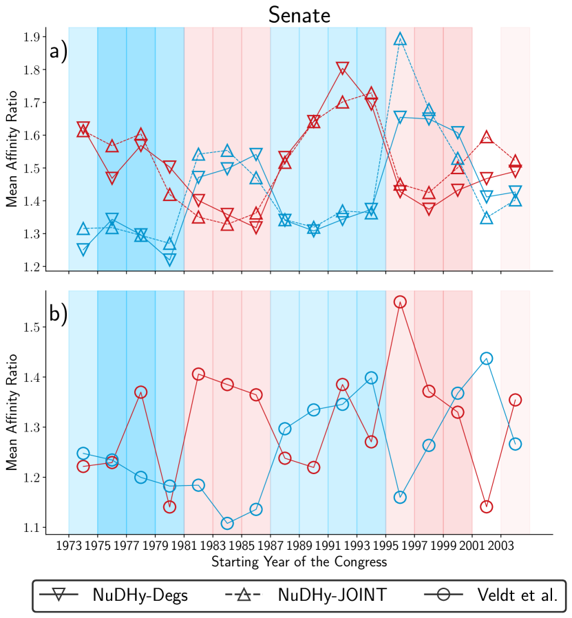
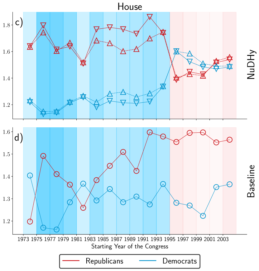
Figure 2: Mean affinity ratios in the US Congress co-sponsored bills. We show results for Equation 3 divided by the mean values in $33$ samples for NuDHy-Degs and NuDHy-JOINT for the US Senate (S-bills), panel (a)) and House (H-bills), panel (c)). For comparison, we show the values of Equation 3 divided by Equation 4 for Veldt et al. again for the US Senate (panel (b)) and House (panel (d)). The colors indicate Democrats (blue) and Republicans (red). We report the average ratios over $k=2,\cdots,14$.

Figure 2 illustrates the mean affinity ratios for Democrats and Republicans in each Congress, for S-bills and H-bills. The mean affinity ratios for NuDHy-Degs and NuDHy-JOINT are computed by averaging the terms $\textsf{A}_{k}(X_{i})/\bar{\textsf{A}}_{k}(X_{i})$ over all hyperedge sizes $k=2,\ldots,14$. The mean affinity ratios for Veldt et al. are obtained by averaging the terms $\textsf{A}_{k}(X_{i})/\textsf{B}_{k}(X_{i})$ over $k=2,\ldots,14$. For each Congress, the background color indicates which party held the majority (shades of red for Republicans and shades of blue for Democrats). The intensity of color corresponds to the size of the majority, with darker shades indicating a larger margin.

These plots show that we can draw similar conclusions when comparing the affinity values against the null models obtained by NuDHy-Degs and NuDHy-JOINT, whereas the baseline scores offer divergent insights. The panels corresponding to NuDHy-Degs/NuDHy-JOINT reveal a clear trend (Figure 2a-c): when one party holds the majority of the seats (indicated by the corresponding color in the background), the opposing party exhibits higher group affinity. This pattern indicates a more unified front, likely in pursuit of collecting the required minimum support to pass their bills.

In instances where Republicans held the majority, Democrats consistently maintained a group affinity $40\%$ to $60\%$ higher than expected, with the exception of the $104^{\mathrm{th}}$ Senate Congress, coinciding with the first occurrence of a Republican majority in both chambers since 1953 and a government shutdown in the US. Conversely, during Democratic majority periods, Republicans exhibited notably higher group affinity, particularly leading up to the $104^{\mathrm{th}}$ session, and especially in the House. Data shows a lower number of bills sponsored by Republicans and a tendency to co-sponsor fewer bills. However, when they decide to co-sponsor a bill, it is more likely to be a bill presented by a Republican. This pattern is consistent with past observations that “Republicans have consistently valued doctrinal purity over pragmatic deal-making”  (?).

In contrast, the baseline yields generally lower affinity values and tends to attribute higher group affinity to the Republicans party, irrespective of the time period. An exception is evident in the $107^{\mathrm{th}}$ Senate Congress starting in 2001, where the mean affinity ratio for Republicans only slightly surpasses $1$, whereas the ratio for Democrats is roughly $1.45$. During this session of the Congress, there is a discernible disparity in co-sponsorship tendencies between Republicans and Democrats. On average, a Republican member tended to co-sponsor fewer bills, averaging around $119$, while their Democratic counterparts engaged in a higher rate of co-sponsorship, averaging around $195$ bills. The baseline score, which fails to consider each party’s relative prevalence and each legislator’s individual co-sponsoring opportunities, inadequately acknowledges the significance of Republican co-sponsoring behaviors for bills sponsored by Republicans versus those sponsored by Democrats. Our null models, instead, maintain these characteristics of the data intact, while randomizing the rest.

In addition, we also found a clear shift in co-sponsoring behavior within the House around the $104^{\mathrm{th}}$/$105^{\mathrm{th}}$ Congress (1995/1997). During this period, Democrats began to consistently co-sponsor a greater number of bills sponsored by Democrats compared to Republicans (see Table 2 in Appendix D), possibly hoping to increase the likelihood of the bills being passed. NuDHy effectively models this shift, as reflected in the corresponding mean affinity ratios.

Party homophily has been studied also by Neal et al.  (?). They represent bill co-sponsorship data as a unipartite weighted graph, where legislators serve as nodes and edge weights indicate the number of bills co-sponsored by pairs of legislators. To ascertain statistically significant connections, they employ a stochastic degree sequence model (SDSM). Despite using a data model that overlooks higher-order relations between legislators and using a simplified analytical framework (a thresholded weighted graph)  (?), they find results akin to our analysis. Specifically, both studies find evidence for differential homophily: the strength of Republicans’ preference for collaborating with other Republicans differs from the strength of Democrats’ preference for collaborating with other Democrats.

Differently from Neal et al., our work remains faithful to the original data. Moreover, the use of randomized networks drawn from ensembles that retain some of the properties of the observed network is more suitable for identifying statistically significant connections  (?).

Finally, the results concerning Equation 5 are presented in Section G.6. We observe that both parties exhibit an inclination toward associating with similar party members in co-sponsorship relations, and that the inverse relationship between the curves of Republicans and Democrats remains discernible, a pattern that remains unnoticed when solely examining the values of $\mathsf{m}$ measured in the observed hypergraphs.

3.2 Contagion Processes in Contact Hyper-Networks

The spread of information or diseases often transcends pairwise interactions and necessitates models that consider the collective influence of groups of individuals. For example, in the context of social and behavioral contagion, multiple studies have shown that exposure to multiple sources can be required  (?, ?). Models of such complex contagion processes aim to capture group influences in social phenomena, such as norm adoption, rumor spread, and disease transmission. These models embrace nonlinear connections between infection rates and sources of infection, which allows for mechanisms such as social reinforcement where multiple (or group) exposures have a larger collective impact than their sum.

More recently, multiple studies have proposed higher-order contagion models describing not only repeated interactions but rather genuine group interactions among agents. In these models, the substrates over which the process evolves are simplicial complexes  (?), undirected hypergraphs  (?, ?), and directed hypergraphs featuring single-node tails  (?). In particular, undirected hypergraphs and simplicial complexes have proven more effective in modeling higher-order interactions between individuals. Conversely, single-tailed directed hypergraphs better model group influences on individuals. The dynamic evolution of such contagion models is typically studied numerically on real-world hyper-networks, and compared to results obtained (both numerically and analytically) for the same dynamics on random hyper-networks  (?, ?, ?). To date, however, it is not clear what are the minimal constraints on such random hyper-networks required to reproduce the dynamical outcomes observed on the real-world hypergraphs. Here, using NuDHy, we highlight the role of structural correlations in shaping the dynamical outcomes of contagion processes. In particular, we show that stronger constraints (as implemented by NuDHy-JOINT) are required to faithfully reproduce results of super-linear contagion dynamics, while looser constraints on degrees and tail/head sizes (NuDHy-Degs) are sufficient when the dynamics is pairwise (linear).

We consider a hypergraph SIS contagion model  (?) wherein the infection rate is a super-linear function of the number of infected nodes in the hyperedges. Let $e$ be a hyperedge and $i_{e}$ be the number of infected nodes in $e$. Then, each of the susceptible nodes in $e$ gets infected at rate $\beta(i_{e})=\lambda i_{e}^{\nu}$, where $\nu$ is a parameter to regulate the non-linearity of the contagion process. The model assumes that infections from different hyperedges are independent processes, and thus defines the total transition rate to the infected state of a node $v$ as the sum of the infection rates of all the hyperedges $E(v)$ containing $v$, i.e., $\sum\limits_{e\in E(v)}\beta(i_{e})$. Let $\mu$ denote the recovery rate (we set $\mu=1$ in all the experiments). Nodes undergo multiple transitions between susceptible and infected states. The contagion process is simulated using a Gillespie algorithm  (?). Starting with an initial density $\rho_{0}$ of infected nodes, the process unfolds via the two types of events (infection and recovery) occurring with probabilities proportional to their respective rates. Once a hyperedge is selected for an infection event, a susceptible node in the hyperedge is chosen uniformly at random to transition to the infected state. To obtain the density of infected nodes in the stationary state, we let the system evolve over a burn-in period $\tau_{b}=10$k. Then, we sample $s=10$k states separated by a decorrelation period $\tau_{d}=1$. Finally, we measure the mean and standard deviation of the density of infected nodes in these samples.

We compare the results of the simulations in the observed hypergraphs and the samples generated by NuDHy with the output of group-based approximate master equations (AMEs) that consider the ensemble of hypergraphs with the same distribution of hyperedge sizes and node degrees  (?). We investigate two scenarios. The first scenario involves undirected hypergraphs depicting face-to-face interactions among children in a primary school in Lyon, France  (?) (lyon) and among students in a high school in Lycée Thiers, France  (?) (high). These hypergraphs are characterized by nearly homogeneous hyperedge size distributions (between 60-70% of the hyperedges have size $2$ and between 15-20% of the hyperedges have size $3$) and bell-shaped node degree distributions centered around $11.79$ and $55.63$, respectively. The second scenario involves email exchanges between members of a European research institution (email-EU) and between Enron employees (email-Enron)  (?). These hypergraphs are characterized by heterogeneous hyperedge size distributions with mean hyperedge size $3$ and $3.42$, respectively, and max hyperedge size $18$ and $25$, respectively. The node degree distributions follow a heavy-tailed distribution. The main characteristics of the four hypergraphs are reported in Table 3 in Appendix D.

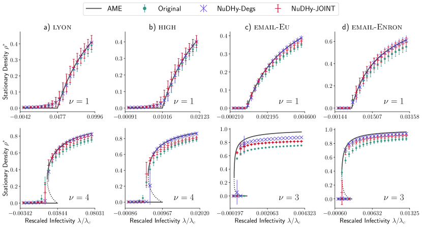
Figure 3: Density of infected nodes in contact networks. We show the values of $\rho^{*}$ in the stationary state of contagion dynamics on the observed hypergraph, and on $33$ samples generated by NuDHy-Degs and NuDHy-JOINT, varying infection rate $\lambda$ and non-linearity parameter $\nu$, for lyon, high, email-Eu, and email-Enron. We report also the output of the AMEs as defined in  (?). The infection rate is rescaled with the invasion threshold $\lambda_{c}$. Errors bars correspond to one standard deviation.

Figure 3 display the average fraction $\rho^{*}$ of infected nodes in the stationary state of contagion dynamics on the observed hypergraphs and on $33$ samples generated by NuDHy-Degs and NuDHy-JOINT, using $\rho_{0}=0.01$, and varying infection rate $\lambda$ and parameter $\nu$. The phase diagram reports also the output of the AMEs. The infection rate is rescaled with the invasion threshold $\lambda_{c}$, which is the minimum $\lambda$ above which the healthy state ($\rho^{*}=0$) is unstable. We consider both linear ($\nu=1$) and super-linear ($\nu>1$) contagions. In the case of linear contagions, we observe two solutions for the stationary fraction of infected nodes: $\rho^{*}_{1}=0$ (absorbing state) and $\rho^{*}_{2}>0$ (endemic state). For the case of super-linear contagions, we chose a value of $\nu$ greater than the bistability threshold $\nu_{c}$ reported in Table 3. The bistability threshold is the smallest non-linear exponent allowing for a discontinuous phase transition. In this case we observe three solutions: $\rho^{*}_{1}=0$ and $\rho^{*}_{3}>0$, which are locally stable, and $0<\rho^{*}_{2}<\rho^{*}_{3}$, which is unstable (dashed lines). To obtain the lower branches in panels c and d in Figure 3 we run the ordinary simulation method described above. On the other hand, the upper branches in panels c and d and the branches in panels a and b are obtained with a quasi-stationary-state method  (?): we keep a history of $50$ past states from which a random state is used to replace the current state each time the absorbing state is reached.

Especially in the smaller datasets and for linear contagion processes, results for NuDHy-Degs align well with the output of the analytical framework. This is expected given that NuDHy-Degs samples uniformly from the ensemble of hypergraphs with the same head and tail size sequences and the same in- and out-degree sequences, which are equivalent to the hyperedge size sequence and the node degree sequence when the input is an undirected hypergraph. The disparities observed in the super-linear processes may potentially be attributed to a too-small value assigned to $\tau_{b}$.

In contrast, the structural correlations present in the observed data lead to reductions in the stationary prevalence compared to the output of the AMEs. These deviations display greater magnitude in the outputs of the super-linear contagions and in the presence of unstable regions, thus suggesting a higher influence of structural correlations within this type of contagion process. Previous works  (?) has shown that the correlations are especially important in the presence of nodes with large degrees. In line with these works, we observe smaller discrepancies in lyon, where node degrees are more homogeneous. Conversely, the discrepancies in the lower branches in panels a and b in Figure 3 are due to the simulations being affected by finite-size effects—while AMEs assume an infinite-size system—and they become higher for the super-linear processes.

By looking at the curves for NuDHy-JOINT in email-Eu and high, we observe that part of the deviation in the super-linear simulations can be explained by the joint degree distribution.

In conclusion, our analysis shows that the fidelity to the original dynamics increases with the amount of preserved structural correlations, with NuDHy-JOINT offering the closest approximation, and the AME being the least accurate. While both NuDHy-Degs and NuDHy-JOINT closely match the real dynamics for linear processes in smaller datasets, discrepancies emerge between their predictions in super-linear processes, with NuDHy-JOINT better approximating the real dynamics. This result highlights the role of higher-order structural correlations in non-linear contagion models, and thus highlights the importance of preserving the joint degree tensor when strongly non-linear processes or strong degree correlations are present (e.g. email-Eu and high).

3.3 Economic Competitiveness in Trade Hyper-Networks

Economic complexity metrics are indicators that aim to capture the diversity and sophistication of a country’s economy through its exported product basket. The diversity and composition of a country’s exported product basket, along with the complexity of the products therein, are the key properties exploited by these metrics to asses the competitiveness of countries. In this analysis, we gauge the relative economic competitiveness of countries via three of these metrics: the Economic Complexity Index (ECI)  (?), the Fitness  (?, ?, ?), and the GENeralised Economic comPlexitY index (GENEPY)  (?). We apply NuDHy alongside three additional null models purposefully designed for directed hypergraphs, with the aim to investigate which characteristics of the observed data are sufficient to replicate the ranking of countries based on these metrics.

Each of the three metrics is defined on an unweighted bipartite graph that represents the export relationships between countries and products: the bipartite country-product network. Nodes of one set represent countries, and nodes of the other set represent products. Unweighted and undirected edges connect countries to their exported products. Following previous literature in this field, we consider a country to be an exporter of a product if its Revealed Comparative Advantage (RCA)  (?) is greater than or equal to a minimum threshold $R^{*}$. RCA measures the relative monetary importance of a product for a country among the export basket of the country compared to the global average. We follow the standard economics literature and set $R^{*}=1.0$  (?). An RCA value greater than $R^{*}$ implies that the given country is advanced enough to compete in the global market for that product. In addition, following the Atlas of Economic Complexity  (?), we only consider countries with a population above $1$ million and an average trade above $1$ billion USD.

Let $\mathsf{M}$ be the biadjacency matrix of the bipartite country-product network defined according to these criteria, and let $\mathsf{W}$ be a transformation matrix defined as $\mathsf{W}[c,p]=\mathsf{M}[c,p]/k_{c}h_{p}$, where $k_{c}$ is the degree of the left vertex $c$ (representing a country), and $h_{p}=\sum_{c}\mathsf{M}[c,p]/k_{c}$. The country-to-country proximity matrix between countries is then defined as follows:

$$\mathsf{X}[c,c^{*}]=\begin{cases}\sum_{p}\mathsf{W}[c,p]\mathsf{W}[c^{*},p]&\text{ if }c\neq c^{*},\\ 0&\text{ if }c=c^{*}.\end{cases}$$

The symmetric matrix $\mathsf{X}$ quantifies the similarities in the export baskets of countries. Let us now recall the three metrics under study.

The Economic Complexity Index (ECI) measures a country’s complexity as the average complexity of the products it exports, and the complexity of a product as the average complexity of the countries that export it. Thus, countries with a high ECI boast diversified export portfolios, featuring unique and sophisticated products, while those with a lower ECI export a more limited selection of common goods. In terms of the biadjacency matrix $\mathsf{M}$, the ECI of a country and the Product Complexity Index (PCI) of a product are defined by the following coupled equations:

$$\mathsf{ECI}(c)=\frac{1}{\sum_{p}\mathsf{M}[c,p]}\sum_{p}\mathsf{M}[c,p]\mathsf{PCI}(p),$$ (6)

$$\mathsf{PCI}(p)=\frac{1}{\sum_{c}\mathsf{M}[c,p]}\sum_{c}\mathsf{M}[c,p]\mathsf{ECI}(p).$$ (7)

The ECI index also possesses an alternative equivalent definition in terms of the eigenvector corresponding to the second largest eigenvalue of the country-to-country proximity matrix $\mathsf{X}$  (?).

The Fitness $\mathsf{F}(c)$ of a country $c$ and the Quality $\mathsf{Q}(p)$ of a product $p$ are defined according to the following coupled equations  (?):

$$\begin{dcases}\widetilde{\mathsf{F}}(c)^{(n)}&=\sum_{p}\mathsf{M}[c,p]\mathsf{Q}(p)^{(n-1)}\\ \widetilde{\mathsf{Q}}(p)^{(n)}&=\frac{1}{\sum_{c}\mathsf{M}[c,p]\frac{1}{\mathsf{F}(c)^{(n-1)}}}\end{dcases}\rightarrow\begin{dcases}\mathsf{F}(c)^{(n)}&=\frac{\widetilde{\mathsf{F}}(c)^{(n)}}{\langle\widetilde{\mathsf{F}}(c)^{(n)}\rangle_{c}}\\ \mathsf{Q}(p)^{(n)}&=\frac{\widetilde{\mathsf{Q}}(p)^{(n)}}{\langle\widetilde{\mathsf{Q}}(p)^{(n)}\rangle_{p}}\end{dcases}$$ (8)

where $\langle\cdot\rangle_{x}$ denotes the arithmetic mean over the distribution of values for $x$. The main difference introduced by the Fitness/Quality scores lies in a non-linear weighting of the fitness of the countries when computing the quality of a product, rather than using a simple average. Fitness and Quality can be computed by solving Equation 8 with an iterative algorithm, initializing $\mathsf{F}(c)^{(0)}=1$ for each country $c$, and $\mathsf{Q}(p)^{(0)}=1$ for each product $p$. The iterative algorithm converges to a single fixed point independently from the initial conditions  (?, ?, ?).

Finally, the GENEPY index is a combination of the eigenvectors of the country-to-country proximity matrix $\mathsf{X}$. More precisely, the GENEPY index of a country $c$ is defined as

$$\mathsf{G}(c)=\left(\sum_{i=1}^{2}\lambda_{c,i}\mathsf{e}_{c,i}^{2}\right)^{2}+2\sum_{i=1}^{2}\lambda_{c,i}^{2}\mathsf{e}_{c,i}^{2}\,,$$ (9)

where $\lambda_{c,i}$ is the $i$-th largest eigenvalue of the proximity matrix $\mathsf{X}$, and $\mathsf{e}_{c,i}$ is the corresponding eigenvector.

As a preliminary observation, note that the bipartite country-product network inherently represents a high-order structure  (?), as any hypergraph can be represented as a bipartite graph without loss of information. Therefore, computing metrics on the bipartite country-product network corresponds to conducting higher-order analyses.

We perform a comparative analysis of country rankings based on ECI, Fitness, and GENEPY computed from the observed data and from $33$ samples generated by NuDHy. We consider international trade data for four years: 1995 (first year available), 2009 (global financial crisis), 2019 (COVID-19 outbreak), and 2020 (economic recession)  (?). We consider a directed higher-order data representation where nodes represent countries and hyperedges represent products traded by them. Coherently with the construction of the bipartite country-product network, the head of each hyperedge includes countries that export the product with a Revealed Comparative Advantage  (?) greater than $1$; the tail of each hyperedge includes countries that import the product with an RCA greater than $1$; and we only consider countries with a population above $1$ million and an average trade above $1$ billion USD. Table 4 in Section G.7 reports the characteristics of the resulting hypergraphs. This directed hypergraph encoding perfectly represents the trade data and offers opportunities for studying the system more thoroughly. For instance, while the country-product network only looks at the export side of the trades, the directed hypergraph also represents imports. Higher-order representations thus offer a richer and more detailed description of the system on which more powerful metrics can be defined (although this specific task is outside the scope of the current work).

Table 1: Average Spearman’s correlation and Kendall’s Tau (KT) of the rankings of the countries obtained according to ECI/Fitness/GENEPY in $33$ samples with respect to the observed rankings, for hs2019. Standard deviations are reported in parentheses.

Score	Metric	Base	BaseD	Null	NuDHy-Degs	NuDHy-JOINT
ECI	Spearman	-0.144 (0.143)	-0.055 (0.120)	0.007 (0.093)	0.020 (0.121)	0.964 (0.001)
	KT	-0.092 (0.092)	-0.037 (0.079)	0.005 (0.062)	0.015 (0.082)	0.848 (0.004)
Fitness	Spearman	0.051 (0.075)	0.237 (0.055)	-0.013 (0.075)	0.981 (0.001)	0.998 (0.000)
	KT	0.034 (0.051)	0.160 (0.038)	-0.010 (0.052)	0.886 (0.003)	0.963 (0.001)
GENEPY	Spearman	0.015 (0.078)	0.230 (0.054)	-0.002 (0.097)	0.941 (0.004)	0.993 (0.000)
	KT	0.010 (0.054)	0.156 (0.040)	-0.001 (0.040)	0.801 (0.007)	0.937 (0.002)

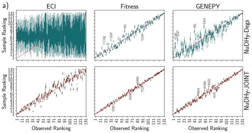
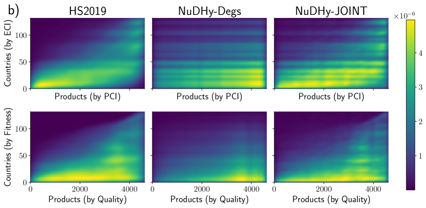
Figure 4: Relative competitiveness in hs2019. Panel a): rankings distributions based on ECI, Fitness, and GENEPY across 33 samples for NuDHy-Degs (top) and NuDHy-JOINT (bottom) compared to the observed rankings, with annotated top-$4$ diverging ranks. Panel b): density plots of the KDE of the observed biadjacency matrix $\mathsf{M}$ and of the aggregated matrices across $33$ samples of NuDHy-Degs and NuDHy-JOINT. Countries are sorted by ECI/Fitness and products by PCI/Quality (descending). The lighter the color, the higher the density of edges.

An analysis similar to ours was presented in a previous study  (?) by employing the Fitness score and the BiCM null model  (?) for the bipartite country-product network. This null model maintains both the left and right degree sequences, but only in expectation (canonical ensemble). The study revealed that, in general, for each country, the distribution of its ranks obtained from the samples has a mean value close to the observed rank, and a wide standard deviation. We find a similar, albeit much stronger, result for NuDHy. In the following, we discuss the main findings in hs2019. Results for the other trade networks are qualitatively similar and are reported in Section G.7.

ECI. For NuDHy-Degs, both the Spearman and Kendall’s Tau average correlation values of the rankings of countries are remarkably close to zero, and the standard deviation values for both coefficients are small (Table 1). This result indicates independence between the observed ranking and the rankings provided by the samples. Figure 4a (upper left) shows this pattern: the distributions of the ranks of each country across the samples tend to cluster around mid-ranking positions and exhibit a wide spread, with greater variance at the lower end of the observed ranking. In other words, preserving the degrees via NuDHy-Degs does not preserve the ECI.

In contrast, for NuDHy-JOINT both average correlation coefficients (Spearman and Kendall’s Tau) of the rankings of countries are significantly high ($\geq 0.84$), and the standard deviation values for both coefficients are negligible (Table 1). This observation suggests a dependence between the observed ranking and the rankings provided by the samples, as illustrated by the bottom left plot of Figure 4a. The distributions of the ranks of each country across the samples are aligned with the observed rank of a country and present a narrow spread.

According to these results, preserving the JOINT is sufficient to preserve the ranking of countries based on their ECI score, while the degree sequence is insufficient.

Fitness and GENEPY. These two measures behave quite similarly in our analysis. For NuDHy-Degs, the average correlation coefficients (Spearman and Kendall’s Tau) of the rankings of countries are significantly high for both Fitness ($\geq 0.88$) and GENEPY ($\geq 0.8$), and the standard deviation values for both coefficients are negligible (Table 1). This result indicates a dependence between the observed rankings and the rankings provided by the samples. The middle and right plots of Figure 4a show that the distributions of the ranks of each country across the samples tend to be close to the observed rank of a country with a narrow spread.

For NuDHy-JOINT, the average correlation coefficients (Spearman and Kendall’s Tau) of the rankings of countries are even higher ($\geq 0.96$ for Fitness and $\geq 0.93$ for GENEPY), and the standard deviation values for both coefficients are extremely small (Table 1). There is a strong dependence between the observed ranking and the rankings provided by the samples, as shown by the bottom middle and right plots of Figure 4a. The distributions of the country rank across the samples are aligned with the observed rank of a country, with a very limited spread.

According to these results, both the degree and joint degree sequence are sufficient to retain the ranking of countries based on their Fitness and GENEPY scores.

Figure 4b displays density plots representing Kernel Density Estimations (KDEs) of the biadjacency matrices for the country-product network of $2019$. These matrices are derived from the observed data (first column) and from the aggregation of $33$ samples generated by NuDHy-Degs and NuDHy-JOINT (second and third column). Countries and products are arranged in descending order of ECI/Fitness and PCI/Quality, respectively. The color intensity within each plot indicates the density of edges, with lighter colors indicating higher density.

As expected, countries with a high Fitness/ECI predominantly export products with high Quality/PCI, while those with lower Fitness/ECI focus solely on products with lower Quality/PCI. Comparison with the corresponding plots for NuDHy-Degs (middle columns of Figure 4b) indicates that the specialization process of countries cannot be fully explained by node degrees alone, as evidenced by the inability of NuDHy-Degs to accurately capture the pattern observed in the real data. Conversely, plots derived from samples of NuDHy-JOINT reveals remarkably similar edge density distributions to those observed, regardless of the metrics used to sort rows and columns (first and third columns of Figure 4b).

Overall, we find that preserving local properties of the hypergraph, either the degree sequences and hyperedge sizes in the case of NuDHy-Degs or their joint tensor for NuDHy-JOINT, is sufficient to explain the rankings induced by most economic complexity measures. As a consequence, it is likely that these measures primarily capture local network structure and do not fully leverage meso- and global-scale information. Our suite of null models NuDHy can help explore the power of these structural metrics, and possibly develop more comprehensive ones that can leverage the natural higher-order representation of the underlying trade data.

Other null models. In this experiment, we also compare our null models with three null models for directed hypergraphs named Base, BaseD, and Null. Base and BaseD are two different versions of ReDi  (?): the first realistic generative model specifically designed for directed hypergraphs. ReDi extends the preferential attachment model  (?) to directed hypergraphs, allowing the generation of random hypergraphs exhibiting reciprocal patterns akin to those observed in real directed hypergraphs. The random hypergraphs generated by this model preserve, on average, the distribution of head and tail sizes. The version of ReDi dubbed Base preserves, on average, the distribution of the number of hyperedges in which each group of nodes appears, while the version dubbed BaseD preserves node degrees on average. Null is a naive sampler that preserves the head and tail size distributions, but populates the hyperedges of the random hypergraph by drawing nodes uniformly at random from the set of nodes of the observed hypergraph. Additional details on these models are provided in Appendix E.

According to the results reported in Table 1, none among Base, BaseD, and Null, can explain the ranking of countries based on these three indexes.

4 Discussion

In this study, we introduced a suite of null models for directed hypergraphs, encompassing hypergraphs with the same in-degree, out-degree, head-size, and tail-size distributions, as well as the same JOINT of an observed hypergraph. We demonstrated a lossless mapping from directed hypergraphs to directed bipartite graphs and proposed two MCMC samplers that efficiently sample from the corresponding micro-canonical graph ensembles.

Our approach fills a critical gap in the existing literature, which primarily focuses on canonical and micro-canonical bipartite graph ensembles  (?, ?, ?, ?, ?, ?, ?, ?) and undirected hypergraph ensembles  (?, ?, ?, ?, ?, ?, ?, ?, ?).

We conducted rigorous experiments and evaluations, highlighting the limitations of recent generative models, such as the one proposed by Kim et al.  (?), specifically designed for directed hypergraphs. The random hypergraphs generated by this (canonical) model preserve, on average, the distribution of head and tail sizes. However, our findings revealed structural dissimilarities between generated hypergraphs and observed ones due to design choices aimed at improving sampler efficiency.

We then showed the importance of preserving stronger structural correlations (and hence the significance of the proposed null models) in three appropriate case studies, spanning various domains. First, we explored group affinity within political parties in the US Congress, revealing an inverse relationship between the affinity curves of Republicans and Democrats: when one party holds the majority of the seats, the opposing party exhibits higher group affinity. This pattern becomes apparent only when the JOINT structural correlations are preserved.

Second, we simulated linear and non-linear contagion processes in real and randomized hyper-networks, demonstrating the explanatory power of the JOINT in elucidating observed discrepancies between analytical contagion frameworks and simulations in real data. These results also suggest that our models could be used for more realistic data augmentation.

Third, we compared the rankings of countries based on three economic complexity indices (ECI, Fitness, and GENEPY) computed in trade hyper-networks and their randomized counterparts, highlighting the nuanced information encoded in the degree sequences and the JOINT. Our analysis revealed that both our null models accurately replicate the relative economic competitiveness of countries as measured by Fitness and GENEPY. However, for ECI, only the more restrictive null model NuDHy-JOINT succeeded in preserving the rankings. These results demonstrate that retaining the local topological properties independently is insufficient to preserve the ranking of the countries based on their ECI score. However, in all three cases, the local properties preserved by NuDHy-JOINT are sufficient to reproduce and explain the rankings, thus indicating that the metrics ignore mesoscale and global properties of the network.

Our findings emphasize the versatility and effectiveness of our proposed null models and samplers in uncovering intricate patterns across diverse disciplines. These tools represent a powerful lens through which to examine higher-order complex systems. They fill a significant gap in the analysis of higher-order networks, thus providing researchers in fields such as neuroscience, ecology, sociology, and economics with effective means for analysis and interpretation. Moreover, thanks to the efficiency of our samplers, our work empowers researchers to glean deeper insights also from more complex and larger datasets. Finally, from a theoretical perspective, our results provide direct motivation for extending analytical descriptions of hyper-networks—and of processes taking place on them—to include more nuanced structural correlation patterns.

5 Sampling Algorithms

This section describes two efficient sampling algorithms, NuDHy-Degs and NuDHy-JOINT, designed for sampling from $\mathcal{Z}^{\textsc{DHCM}}$ and $\mathcal{Z}^{\textsc{DHJM}}$, respectively. Both algorithms leverage the Metropolis-Hastings algorithm as part of the Markov Chain Monte Carlo approach, and employ targeted edge swap operations to traverse the Markov graph. NuDHy-Degs uses Parity Swap Operations (Lemma 1), while NuDHy-JOINT uses Restricted Parity Swap Operations (Lemma 2). The sampling procedures for both algorithms are illustrated through pseudocode and detailed in Appendix B and Appendix C, respectively. Finally, we experimentally study the mixing time of the samplers in Appendix F. The code is publicly available on GitHub.

5.1 NuDHy-Degs: An Efficient Sampler for DHCM

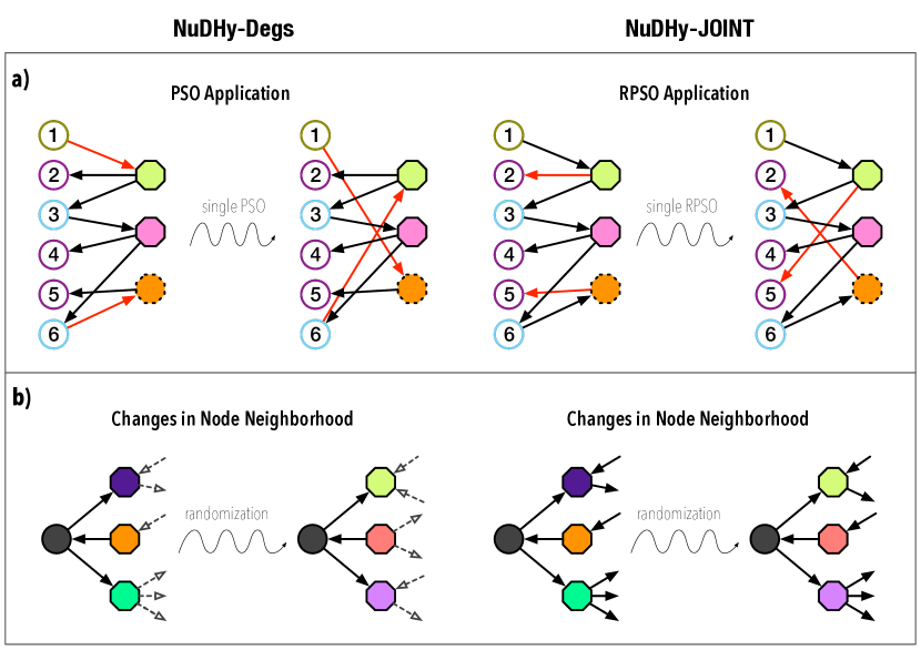
Figure 5: a) Bipartite graphs obtained from Figure 1a after the application of the PSO $(1,\leavevmode\hbox to11.78pt{\vbox to10.26pt{\text{[drawing]}}},+1),(6,\leavevmode\hbox to11.78pt{\vbox to10.26pt{\text{[drawing]}}},+1)\xrightarrow{\mathrm{PSO}}(1,\leavevmode\hbox to11.78pt{\vbox to10.26pt{\text{[drawing]}}},+1),(6,\leavevmode\hbox to11.78pt{\vbox to10.26pt{\text{[drawing]}}},+1)$ and of the RPSO $(2,\leavevmode\hbox to11.78pt{\vbox to10.26pt{\text{[drawing]}}},-1),(5,\leavevmode\hbox to11.78pt{\vbox to10.26pt{\text{[drawing]}}},-1)\xrightarrow{\mathrm{RPSO}}(2,\leavevmode\hbox to11.78pt{\vbox to10.26pt{\text{[drawing]}}},-1),(5,\leavevmode\hbox to11.78pt{\vbox to10.26pt{\text{[drawing]}}},-1)$. The edges involved in the swap operations are highlighted in red. Left nodes with the same in- and out-degree are outlined with the same color. Right nodes with the same in- and out-degree are outlined with the same pattern. b) Changes in the neighborhood of a left node after the application of a sequence of PSOs and of RPSOs. PSOs preserve the number of in-going and out-going edges of each node. RPSOs preserve also the in- and out-degree of the nodes connected to each node.

We present a Markov Chain Monte Carlo algorithm, dubbed NuDHy-Degs, that uses Metropolis-Hastings (MH) to sample from $\mathcal{Z}^{\textsc{DHCM}}$ according to $\pi$. We first define an edge swap operation that transforms a bipartite graph into another bipartite graph while preserving the degree sequences, and then describe the state space that this operation induces and over which the Markov chain is constructed.

Lemma 1 (Parity Swap Operation, PSO).

Let $G\doteq(L,R,D)$ be a directed bipartite graph and $u\neq v\in L$, $\alpha\neq\beta\in R$ such that $\exists d\in\{+1,-1\}$ for which $e_{1}\doteq(u,\alpha,d),e_{2}\doteq(v,\beta,d)\in D$ and $e_{3}\doteq(u,\beta,d),e_{4}\doteq(v,\alpha,d)\notin D$. Swapping $e_{1}$, $e_{2}$ with $e_{3}$, $e_{4}$ generates a directed bipartite graph $G^{\prime}=(L,R,(D\setminus\{e_{1},e_{2}\})\cup\{e_{3},e_{4}\})$ with the same left and right, in- and out-degree sequences as $G$. This swap operation, denoted as $e_{1},e_{2}\xrightarrow{\mathrm{PSO}}e_{3},e_{4}$, is called parity swap operation (PSO).

For directed unipartite graphs, this operation is known as checkerboard swap  (?). An example of PSO is shown in Figure 5a (left).

Algorithm 1 NuDHy-Degs

1:Graph $G\doteq(L,R,D)\in\mathcal{G}^{\textsc{DHCM}}$, Number of Steps $s$

2:Graph sampled uniformly from $\mathcal{G}^{\textsc{DHCM}}$

3:repeat $s$ times

4:    $\mathsf{out}\leftarrow$ flip a biased coin with heads probability $|\overrightarrow{D}|/|D|$

5:    if $\mathsf{out}$ is heads then

6:         $u$, $v$ $\leftarrow$ distinct vertices drawn u.a.r. from $\overrightarrow{L}$ $\triangleright$ vertices in $L$ with out-degree $>0$

7:         if $\mathsf{X}^{+}_{u,v}\neq\varnothing$ then $\triangleright$ $\{(\alpha,\beta)\mathrel{:}\alpha\in\overrightarrow{\Gamma}(u)\setminus\overrightarrow{\Gamma}(v)\,\wedge\beta\in\overrightarrow{\Gamma}(v)\setminus\overrightarrow{\Gamma}(u)\}$

8:             $\alpha$, $\beta$ $\leftarrow$ pair drawn u.a.r. from $\mathsf{X}^{+}_{u,v}$

9:             perform $(u,\alpha,+1),(v,\beta,+1)\xrightarrow{\mathrm{PSO}}(u,\beta,+1),(v,\alpha,+1)$ on $G$          

10:    else

11:         $\alpha$, $\beta$ $\leftarrow$ distinct vertices drawn u.a.r. from $\overleftarrow{R}$ $\triangleright$ vertices in $R$ with out-degree $>0$

12:         if $\mathsf{X}^{+}_{\alpha,\beta}\neq\varnothing$ then $\triangleright$ $\{(u,v)\mathrel{:}u\in\overrightarrow{\Gamma}(\alpha)\setminus\overrightarrow{\Gamma}(\beta)\,\wedge v\in\overrightarrow{\Gamma}(\beta)\setminus\overrightarrow{\Gamma}(\alpha)\}$

13:             $u$, $v$ $\leftarrow$ pair drawn u.a.r. from $\mathsf{X}^{+}_{\alpha,\beta}$

14:             perform $(u,\alpha,-1),(v,\beta,-1)\xrightarrow{\mathrm{PSO}}(u,\beta,-1),(v,\alpha,-1)$ on $G$              

15:return $G$

The state space $\mathcal{G}^{\textsc{DHCM}}$ is a directed weighted graph. Each vertex represents a bipartite directed graph with the same left and right, in- and out-degree sequences as $\mathring{G}$. Each edge connects two graphs that can be transformed into each other via a PSO. For any pair of graphs, there is at most one PSO that connects them, hence there are no parallel edges between vertices. Moreover, we add self-loops from each vertex to itself. All the graphs $G^{\prime}$ that can be obtained by applying a PSO to $G$ are called the neighbors of $G$ in $\mathcal{G}^{\textsc{DHCM}}$. We associate a weight $\xi_{G}(G^{\prime})$ to each edge $(G,G^{\prime})$ that represents the probability of transitioning to $G^{\prime}$ starting from $G$.

A fundamental theorem of Markov chains states that an irreducible, aperiodic, finite Markov chain has a unique stationary distribution  (?). Therefore, the Markov chain converges to $\pi$ independently of the starting state. Furthermore, we know that if the transition probability matrix is doubly stochastic, the Markov chain converges to the uniform distribution over its state space. As a result, samples from the chain can be considered as uniform samples from the state space. In our case, aperiodicity is guaranteed by the presence of self-loops over the vertices, while the double stochasticity of the transition matrix can be inferred from observing that (i) each PSO is reversible, i.e., if $e_{1},e_{2}\xrightarrow{\mathrm{PSO}}e_{3},e_{4}$ transforms $G$ into $G^{\prime}$, then $e_{3},e_{4}\xrightarrow{\mathrm{PSO}}e_{1},e_{2}$ transforms $G^{\prime}$ into $G$; and that (ii) the probability of going from $G$ to $G^{\prime}$ is equal to the probability of going from $G^{\prime}$ to $G$, i.e., $\xi_{G}(G^{\prime})=\xi_{G^{\prime}}(G)$. The definition of $\xi_{G}$ and the proof that the transition matrix $\{\xi_{G}(G^{\prime})\}$ is doubly stochastic can be found in Appendix B. Finally, Appendix A proves irreducibility by showing that $\mathcal{G}^{\textsc{DHCM}}$ is strongly connected. From these results, we obtain that the stationary distribution is the uniform distribution.

Algorithm 1 illustrates the sampling procedure of NuDHy-Degs. The algorithm performs a number of steps $s$ (input parameter) in the state space large enough that its output can be considered as a uniform sample from $\mathcal{G}^{\textsc{DHCM}}$. Previous works has shown that $s=O\left(|E|\log\left(|E|\right)\right)$ is, in general, sufficient  (?).

5.2 NuDHy-JOINT: An Efficient Sampler for DHJM

We introduce an edge swap operation that transforms a bipartite graph into another bipartite graph with the same JOINT.

Lemma 2 (Restricted Parity Swap Operation, RPSO).

Let $G\doteq(L,R,D)$ be a directed bipartite graph and $u\neq v\in L$, $\alpha\neq\beta\in R$ such that $\exists d\in\{+1,-1\}$ for which $e_{1}\doteq(u,\alpha,d),e_{2}\doteq(v,\beta,d)\in D$ and $e_{3}\doteq(u,\beta,d),e_{4}\doteq(v,\alpha,d)\notin D$.

If $\mathsf{ideg}(u)=\mathsf{ideg}(v)\,\wedge\,\mathsf{odeg}(u)=\mathsf{odeg}(v)\;\vee\;\mathsf{ideg}(\alpha)=\mathsf{ideg}(\beta)\,\wedge\,\mathsf{odeg}(\alpha)=\mathsf{odeg}(\beta)$, then swapping $e_{1}$, $e_{2}$ with $e_{3}$, $e_{4}$ generates a directed bipartite graph $G^{\prime}=(L,R,(D\setminus\{e_{1},e_{2}\})\cup\{e_{3},e_{4}\})$ with the same JOINT as $G$. This swap operation, denoted as $e_{1},e_{2}\xrightarrow{\mathrm{RPSO}}e_{3},e_{4}$, is called restricted parity swap operation (RPSO).

An example of RPSO is shown in Figure 5a (right).

Algorithm 2 NuDHy-JOINT

1:Graph $G\doteq(L,R,D)\in\mathcal{G}^{\textsc{DHJM}}$, Number of Steps $s$

2:Graph sampled uniformly from $\mathcal{G}^{\textsc{DHJM}}$

3:repeat $s$ times

4:    $\mathsf{out}\leftarrow$ flip a biased coin with heads prob $|\overrightarrow{D}|/|D|$

5:    $\mathsf{out2}\leftarrow$ flip a fair coin

6:    if $\mathsf{out2}$ is heads then

7:         $u$, $v$ $\leftarrow$ different random left vertices with the same in- and out-degree

8:         if $\mathsf{out}$ is heads and $\mathsf{X}^{+}_{u,v}\neq\varnothing$ then $\triangleright$ $\mathsf{X}^{+}_{u,v}\doteq\{(\alpha,\beta)\mathrel{:}\alpha\in\overrightarrow{\Gamma}(u)\setminus\overrightarrow{\Gamma}(v)\,\wedge\beta\in\overrightarrow{\Gamma}(v)\setminus\overrightarrow{\Gamma}(u)\}$

9:             $\alpha$, $\beta$ $\leftarrow$ pair drawn u.a.r. from $\mathsf{X}^{+}_{u,v}$

10:             perform $(u,\alpha,+1),(v,\beta,+1)\xrightarrow{\mathrm{RPSO}}(u,\beta,+1),(v,\alpha,+1)$ on $G$

11:         else if $\mathsf{out}$ is tails and $\mathsf{X}^{-}_{u,v}\neq\varnothing$ then $\triangleright$ $\mathsf{X}^{-}_{u,v}\doteq\{(\alpha,\beta)\mathrel{:}\alpha\in\overleftarrow{\Gamma}(u)\setminus\overleftarrow{\Gamma}(v)\,\wedge\,\beta\in\overleftarrow{\Gamma}(v)\setminus\overleftarrow{\Gamma}(u)\}$

12:             $\alpha$, $\beta$ $\leftarrow$ pair drawn u.a.r. from $\mathsf{X}^{-}_{u,v}$

13:             perform $(u,\alpha,-1),(v,\beta,-1)\xrightarrow{\mathrm{RPSO}}(u,\beta,-1),(v,\alpha,-1)$ on $G$          

14:    else

15:         $\alpha$, $\beta$ $\leftarrow$ different random right vertices with the same in- and out-degree

16:         if $\mathsf{out}$ is heads and $\mathsf{X}^{-}_{\alpha,\beta}\neq\varnothing$ then

17:             $u$, $v$ $\leftarrow$ pair drawn u.a.r. from $\mathsf{X}^{-}_{\alpha,\beta}$

18:             perform $(u,\alpha,+1),(v,\beta,+1)\xrightarrow{\mathrm{RPSO}}(u,\beta,+1),(v,\alpha,+1)$ on $G$

19:         else if $\mathsf{out}$ is tails and $\mathsf{X}^{+}_{\alpha,\beta}\neq\varnothing$ then

20:             $u$, $v$ $\leftarrow$ pair drawn u.a.r. from $\mathsf{X}^{+}_{\alpha,\beta}$

21:             perform $(u,\alpha,-1),(v,\beta,-1)\xrightarrow{\mathrm{RPSO}}(u,\beta,-1),(v,\alpha,-1)$ on $G$              

22:return $G$

The state space $\mathcal{G}^{\textsc{DHJM}}$ is a directed weighted graph where each vertex is a bipartite directed graph with the same JOINT of $\mathring{G}$, and edges connect graphs that can be transformed into each other via an RPSO. For each pair of vertices, there is at most one RPSO that can transform the first one into the second one, and self-loops are added to guarantee that the Markov chain is aperiodic. Appendix C defines a transition probability distribution $\xi_{G}$ over the set of neighbors of any $G\in\mathcal{G}^{\textsc{DHJM}}$ and proves that $\sum_{G^{\prime}\in\mathcal{G}^{\textsc{DHJM}}}\xi_{G}(G^{\prime})=1$. By observing that each RPSO is reversible and that the number of common in- and out-neighbors between any pair of nodes does not change after the application of an RPSO, we have that $\xi_{G}(G^{\prime})=\xi_{G^{\prime}}(G)$ and that the transition matrix $\{\xi_{G}(G^{\prime})\}$ is doubly stochastic. Finally, in Appendix A we prove irreducibility by showing that $\mathcal{G}^{\textsc{DHJM}}$ is strongly connected. From these results, we obtain that the stationary distribution is the uniform distribution. Algorithm 2 illustrates the sampling procedure of NuDHy-JOINT.

[appendix] [appendix]1

Appendix A Proofs

Lemma 3.

$\mathcal{G}^{\textsc{DHCM}}$ is strongly connected via PSOs.

Proof.

We prove that $\mathcal{G}^{\textsc{DHCM}}$ is strongly connected, by showing that any pair of distinct graphs $G_{1}\doteq(L,R,D_{1})$ and $G_{2}\doteq(L,R,D_{2})$ in $\mathcal{G}^{\textsc{DHCM}}$ can be transformed into one another through a sequence of PSOs.

We recall that PSOs swap only edges with the same direction. Hence, we can independently address the edges in $\overrightarrow{D}_{1}$ and $\overrightarrow{D}_{2}$, and the edges in $\overleftarrow{D}_{1}$ and $\overleftarrow{D}_{2}$. Given $\overrightarrow{D}_{1}$ and $\overrightarrow{D}_{2}$ (resp. $\overleftarrow{D}_{1}$ and $\overleftarrow{D}_{2}$), we construct a canonical path from $\overrightarrow{D}_{1}$ to $\overrightarrow{D}_{2}$ (resp. from $\overleftarrow{D}_{1}$ to $\overleftarrow{D}_{2}$), following the procedure outlined in Section 2.1 of  (?). This canonical path delineates a series of switches, i.e., edge swaps between pairs of edges. Although the original procedure was tailored for undirected bipartite graphs with the same degree distribution, we can extend it to our scenario. Since the edges in $\overrightarrow{D}_{1}$ and $\overrightarrow{D}_{2}$ (resp. $\overleftarrow{D}_{1}$ and $\overleftarrow{D}_{2}$) have the same direction, we can see $(L,R,\overrightarrow{D}_{1})$ and $(L,R,\overrightarrow{D}_{2})$ as undirected bipartite graphs. Consequently, each PSO involving edges in $\overrightarrow{D}_{1}$ and $\overrightarrow{D}_{2}$ (resp. $\overleftarrow{D}_{1}$ and $\overleftarrow{D}_{2}$) corresponds to a switch operation.

Therefore, the sequence of PSOs transforming $G_{1}$ into $G_{2}$ simply consists in the concatenation of the switch sequence from $\overrightarrow{D}_{1}$ to $\overrightarrow{D}_{2}$, and the switch sequence from $\overleftarrow{D}_{1}$ to $\overleftarrow{D}_{2}$. ∎

Lemma 4.

$\mathcal{G}^{\textsc{DHJM}}$ is strongly connected via RPSOs.

Proof.

We prove that $\mathcal{G}^{\textsc{DHJM}}$ is strongly connected, by adapting the proof for the case of undirected bipartite graphs, proposed in  (?). Let $\mathcal{C}$ be the list of distinct tuples of in- and out-degrees of nodes in $G$, i.e., $c_{i}\doteq(k,l)$ iff $\exists v\in L,R\mathrel{:}\mathsf{ideg}(v)=k\wedge\mathsf{odeg}(v)=l$. We define the degree spectrum of $v\in L,R$ as the vector $s_{G}(v)$ where $s_{G}(v)[i]$ is the number of vertices with in-degree $c_{i}[0]$ and out-degree $c_{i}[1]$ to which $v$ is connected. We partition $L$ into $V^{L}_{1},\dots,V^{L}_{|\mathcal{C}|}$ such that each $V^{L}_{i}$ contains the vertices in $L$ with in-degree $c_{i}[0]$ and out-degree $c_{i}[1]$. Similarly, we partition $R$ into $V^{R}_{1},\dots,V^{R}_{|\mathcal{C}|}$.

For each $j$ such that $\left|V^{L}_{j}\right|\neq 0$ and each $i$, we set

$$A^{L}_{j}(i)\doteq\frac{\mathsf{T}_{G}[c_{j}[0],c_{j}[1],c_{i}[0],c_{i}[1],+1]}{\left|V^{L}_{j}\right|}\enspace.$$

Similarly, for each $j$ such that $\left|V^{R}_{j}\right|\neq 0$ and each $i$, we set

$$A^{R}_{j}(i)\doteq\frac{\mathsf{T}_{G}[c_{i}[0],c_{i}[1],c_{j}[0],c_{j}[1],-1]}{|V^{R}_{j}|}\enspace.$$

We say that $V^{L}_{j}$ (resp. $V^{R}_{j}$) is balanced in $G$, if it is empty, or for each $V^{R}_{i}$ (resp. $V^{L}_{i}$) the edges connecting $V^{L}_{j}$ to $V^{R}_{i}$ (resp. $V^{R}_{j}$ to $V^{L}_{i}$) are as uniformly distributed on $V^{L}_{j}$ as possible. This happens when for all $v\in V^{L}_{j}$ and all $i$, $s_{G}(v)[i]\in\left\{\left\lfloor A^{L}_{j}(i)\right\rfloor,\left\lceil A^{L}_{j}(i)\right\rceil\right\}$. We say that $G$ is left-balanced (resp. right-balanced) if $V^{L}_{i}$ (resp. $V^{R}_{i}$) is balanced for all $i$. Finally, for each $v\in L$ and $i$ such that $V^{R}_{i}\neq\varnothing$, we define $c^{L}_{G}(v,i)\doteq\left\lfloor\left|A^{L}_{j}(i)-s_{G}(v)[i]\right|\right\rfloor$, where $c_{j}=\left(\mathsf{ideg}(v),\mathsf{odeg}(v)\right)$, and for each $j$ we define $C_{G}^{L}(j)\doteq\sum_{v\in V^{L}_{j}}\sum_{i}c^{L}_{G}(v,i)$. Similarly, for each $v\in R$ and $i$ such that $V^{L}_{i}\neq\varnothing$, we define $c^{R}_{G}(v,i)$ and for each $j$ we define $C_{G}^{R}(j)$.

We observe that we cannot swap two edges $(u,\alpha,d)$ and $(v,\beta,d^{\prime})$ such that $d\neq d^{\prime}$, because the resulting graph would have different in- and out-degree sequences. For example, if $D=\{(u,\alpha,+1)$ , $(v,\beta,-1)\}$, by swapping $(u,\alpha,+1)$ and $(v,\beta,-1)$, the in-degree of $\alpha$ goes from $1$ to $0$, while its out-degree goes from $0$ to $1$. As a result, we can treat the case where we swap edges with direction $1$ and the case where we swap edges with direction $-1$ independently.

To prove that $\mathcal{G}^{\textsc{DHJM}}$ is strongly connected, we first need to prove the following lemma for $C^{L}_{G}$. The proof for $C^{R}_{G}$ follows the same steps.

Lemma 5 (Lemma 4  (?)).

If $C^{L}_{G}(j)\neq 0$, then there exists $u,v\in V^{L}_{j}$ and a RPSO $(u,\alpha,+1)$ , $(v,\beta,+1)$ $\xrightarrow{\mathrm{RPSO}}$ $(u,\beta,+1),(v,\alpha,+1)$ transforming $G$ into $G^{\prime}$ such that $C^{L}_{G^{\prime}}(j)<C^{L}_{G}(j)$ and for all $l\neq j$ $C^{L}_{G^{\prime}}(l)=C^{L}_{G}(l)$.

Proof.

We choose $u,v\in V^{L}_{j}$ such that $s_{G}(u)[i]$ is minimal and $s_{G}(v)[i]$ is maximal among the vertices in $V^{L}_{j}$. Since $u$ has fewer neighbors in $V^{R}_{i}$ than $v$, there exists $\beta\in V^{R}_{i}$ such that $(v,\beta,+1)\in D$ but $(u,\beta,+1)\notin D$. Since $u$ and $v$ have the same out-degrees and $s_{G}(v)[i]>s_{G}(u)[i]$, there exists a $k\neq i$ such that $s_{G}(u)[k]>s_{G}(v)[k]$, and hence there exists $\alpha\in V^{R}_{k}$ such that $(u,\alpha,+1)\in D$ but $(v,\alpha,+1)\notin D$. Therefore, $(u,\alpha,+1)$ , $(v,\beta,+1)\xrightarrow{\mathrm{RPSO}}(v,\alpha,+1)$ , $(u,\beta,+1)$ is a RPSO. Similarly to  (?), by applying such RPSO we obtain a graph $G^{\prime}$ such that $C^{L}_{G^{\prime}}(j)<C^{L}_{G}(j)$. Since the RPSO involves only left nodes with in- and out-degree combination $c_{j}$, all the $C^{L}_{G}(l)$ for $l\neq j$ remain unchanged, i.e., $C^{L}_{G^{\prime}}(l)=C^{L}_{G}(l)$. ∎

Thanks to Lemma 5, we have the following corollary:

Corollary 1 (Corollary 5  (?)).

Given a directed bipartite graph $G\in\mathcal{G}^{\textsc{DHJM}}$, there exists a series of RPSOs transforming $G$ into a left-balanced (resp. right-balanced) graph $G^{\prime}\in\mathcal{G}^{\textsc{DHJM}}$.

Proof.

We follow the proof of  (?), which shows that successive applications of Lemma 5 for each $i$ such that $C^{L}_{G}(i)\neq 0$ (resp. $C^{R}_{G}(i)\neq 0$), give a sequence of RPSOs that transforms $G$ into a left-balanced (resp. right-balanced) graph. ∎

We observe that when balancing the left side of $G$, we do not affect the values $C^{R}_{G}(i)$, and similarly, when balancing the right side of $G$, we do not affect the values $C^{L}_{G}(i)$. As a result, we can first apply Corollary 1 to transform $G$ into a left-balanced graph $G^{\prime}$, and then apply Corollary 1 to transform $G^{\prime}$ into a right-balanced graph $G^{\prime\prime}$ that is left-balanced as well.

To prove that left- and right-balanced graphs can be connected via RPSOs, we first define two auxiliary bipartite graphs $\mathcal{A}^{L}(G,j)\doteq(U^{L},P^{L};E^{L})$ and $\mathcal{A}^{R}(G,j)\doteq(U^{R},P^{R};E^{R})$, such that $U^{L}$ (resp. $U^{R}$) contains a node $u_{v}$ for each $v\in V_{j}^{L}$ (resp. $V_{j}^{R}$), $P^{L}$ (resp. $P^{R}$) contains a node $p_{i}$ for each $V_{i}^{R}$ (resp. $V_{i}^{L}$) such that $A^{L}_{j}(i)\notin\mathbb{N}$ (resp. $A^{R}_{j}(i)\notin\mathbb{N}$), and $E^{L}$ (resp. $E^{R}$) contains an edge $(u_{v},p_{i})$ for each $v$ such that $s_{G}(v)[i]=\lfloor A^{L}_{j}(i)\rfloor+1$ (resp. $s_{G}(v)[i]=\lfloor A^{R}_{j}(i)\rfloor+1$). Then, we define the bipartite swap operation (BSO) as the operation that, given an undirected bipartite graph $B\doteq(V,E)$, takes two edges $(u,a)$, $(v,b)$ $\in E$ such that $(u,b)$, $(v,a)$ $\notin E$, and generates a new bipartite graph $B^{\prime}=(V,E\setminus\{(u,a),(v,b)\}\cup\{(u,b),(v,a)\})$. It can be easily seen that BSOs preserve the left and right degree distributions of $B$.

Graphs in $\mathcal{G}^{\textsc{DHJM}}$ and their auxiliary graphs are linked by the following lemma:

Lemma 6 (Lemma 6  (?)).

If there is a BSO transforming $\mathcal{A}^{L}(G,j)$ (resp. $\mathcal{A}^{R}(G,j)$) into $\mathcal{\hat{A}}^{L}(G,j)$, then there is a RPSO transforming $G$ into $G^{\prime}$ such that $\mathcal{A}^{L}(G^{\prime},j)=\mathcal{\hat{A}}^{L}(G,j)$ (resp. $\mathcal{A}^{R}(G^{\prime},j)=\mathcal{\hat{A}}^{R}(G,j)$), and $s_{G}(v)=s_{G^{\prime}}(v)$ for each vertex $v\notin V_{j}^{L}$ (resp. $v\notin V_{j}^{R}$).

Proof.

We can straightforwardly use the proof in  (?) to prove the lemma for both the $\mathcal{A}^{L}(G,j)$ and the $\mathcal{A}^{R}(G,j)$ case. ∎

Thanks to Lemma 6, we can prove the following theorem, which establishes a relation between any two left-balanced (resp. right-balanced) graphs in $\mathcal{G}^{\textsc{DHJM}}$ :

Theorem 1 (Theorem 7  (?)).

If $G_{1}$ and $G_{2}$ are two left-balanced (resp. right-balanced) graphs in $\mathcal{G}^{\textsc{DHJM}}$, then there is a series of RPSOs transforming $G_{1}$ into $G_{1}^{\prime}$, such that $s_{G_{1}^{\prime}}(v)=s_{G_{2}}(v)$ for each $v\in L$ (resp. $v\in R$).

Proof.

We prove the theorem for the left-balanced case. The other case can be handled in a similar way. We construct a sequence of graphs $G^{0}_{1},G^{1}_{1},G^{2}_{1},\dots,G^{|\mathcal{C}|}_{1}$ with $G_{1}^{0}=G_{1}$ such that for each $i$ there is a sequence of RPSOs transforming $G^{i-1}_{1}$ to $G^{i}_{1}$ such that $s_{G^{i}_{1}}(v)=s_{G_{2}}(v)$ for each $v\in V^{L}_{i}$ and $s_{G^{i}_{1}}(v)=s_{G^{i-1}_{1}}(v)$ for each $v\notin V^{L}_{i}$. Since (i) all the vertices in $V^{L}_{i}$ have the same out-degree and (ii) $G_{1}$ and $G_{2}$ have the same JOINT, we have that $\mathcal{A}^{L}(G^{i-1}_{1},i)$ and $\mathcal{A}^{L}(G_{2},i)$ have the same degree sequences. Therefore, we can apply the Ryser’s Theorem  (?) to obtain a sequence of BSOs transforming one into the other. Thanks to Lemma 6, we know that there exists a sequence of RPSOs transforming $G_{1}^{i-1}$ into the desired $G^{i}_{1}$. The proof concludes by setting $G_{1}^{\prime}=G^{|\mathcal{C}|}_{1}$. ∎

Given two left- and right-balanced graphs $G_{1}$ and $G_{2}$, we can apply Theorem 1 two times: the first application transforms $G_{1}$ into $G_{1}^{\prime}$ such that $s_{G_{1}^{\prime}}(v)=s_{G_{2}}(v)$ for each $v\in L$, while the second application transforms $G_{1}^{\prime}$ into $G_{1}^{\prime\prime}$ such that $s_{G_{1}^{\prime\prime}}(v)=s_{G_{2}}(v)$ for each $v\in R$. We observe that the second application of the theorem does not affect the values $s_{G_{1}^{\prime}}(v)$ for $v\in L$ because it acts only on the outgoing edges of nodes in $R$.

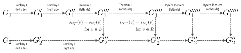
Figure 6: Steps to prove that $\mathcal{G}^{\textsc{DHJM}}$ is strongly connected.

We can now prove that $\mathcal{G}^{\textsc{DHJM}}$ is strongly connected. The main steps of the proof are illustrated in Figure 6. Let $G_{1}$ and $G_{2}$ two non-isomorphic graphs in $\mathcal{G}^{\textsc{DHJM}}$. We apply Corollary 1 two times to transform $G_{1}$ and $G_{2}$ into left- and right-balanced graphs $G_{1}^{\prime\prime}$ and $G_{2}^{\prime\prime}$. Next, we apply Theorem 1 to transform $G_{1}^{\prime\prime}$ into a left-balanced realization $G_{1}^{\prime\prime\prime}$ such that $s_{G_{1}^{\prime\prime\prime}}(v)=s_{G_{2}^{\prime\prime}}(v)$ for each $v\in L$. Next, we we apply Theorem 1 to transform $G_{1}^{\prime\prime\prime}$ into a left- and right-balanced realization $G_{1}^{\prime\prime\prime\prime}$ such that $s_{G_{1}^{\prime\prime\prime\prime}}(v)=s_{G_{2}^{\prime\prime}}(v)$ for each $v\in R$. We note that, the application of the theorem on the right side does not affect the values $s_{G_{1}^{\prime\prime\prime}}(u)$ for $u\in L$, and hence $G_{1}^{\prime\prime\prime\prime}$ is both left and right-balanced. For $i,j$, let $G_{1,L}^{ij}$ and $G_{2,L}^{ij}$ the bipartite graphs consisting of edges in $G_{1}^{\prime\prime\prime\prime}$ and $G_{2}^{\prime\prime}$, respectively, from vertices in $V^{L}_{i}$ to vertices in $V^{R}_{j}$. Similarly, let $G_{1,R}^{ij}$ and $G_{2,R}^{ij}$ the bipartite graphs consisting of edges in $G_{1}^{\prime\prime\prime\prime}$ and $G_{2}^{\prime\prime}$, respectively, from vertices in $V^{R}_{i}$ to vertices in $V^{L}_{j}$. Let $T\in\{L,R\}$. Since $s_{G_{1}^{\prime\prime\prime\prime}}(v)=s_{G_{2}^{\prime\prime}}(v)$ for all $v\in T$, the degree sequences of $G_{1,T}^{ij}$ and $G_{2,T}^{ij}$ are the same. Moreover, since all the left vertices in $G_{1,T}^{ij}$ and $G_{2,T}^{ij}$ have the same combination of in- and out-degree, a BSO in $G_{1,T}^{ij}$ is a RPSO in $G_{1}^{\prime\prime\prime\prime}$. Therefore, for each $i,j$ and each $T\in\{L,R\}$, we can apply the Ryser’s theorem  (?) to obtain a sequence of BSOs transforming $G_{1,T}^{ij}$ into $G_{2,T}^{ij}$, hence obtaining a sequence of RPSOs transforming $G_{1}^{\prime\prime\prime\prime}$ into $G_{2}^{\prime\prime}$. ∎

Appendix B Algorithmic Details of NuDHy-Degs

Let $\overrightarrow{L}\doteq\{v\in L\mathrel{:}\mathsf{odeg}_{G}(v)>0\}$ the subset of left vertices with out-going edges, $\overleftarrow{R}\doteq\{\alpha\in R\mathrel{:}\mathsf{odeg}_{G}(\alpha)>0\}$ the subset of right nodes with out-going edges, and $\mathsf{X}^{+}_{u,v}\doteq\{(\alpha,\beta)\mathrel{:}\alpha\in\overrightarrow{\Gamma}(u)\setminus\overrightarrow{\Gamma}(v)\,\wedge\beta\in\overrightarrow{\Gamma}(v)\setminus\overrightarrow{\Gamma}(u)\}$ be the set of pairs of out-neighbors of $u$ and $v$ that are not out-neighbors of $v$ and $u$, respectively.

Algorithm 3 NuDHy-Degs

1:Graph $G\doteq(L,R,D)\in\mathcal{G}^{\textsc{DHCM}}$, Number of Steps $s$

2:Graph sampled uniformly from $\mathcal{G}^{\textsc{DHCM}}$

3:repeat $s$ times

4:    $\mathsf{out}\leftarrow$ flip a biased coin with heads probability $|\overrightarrow{D}|/|D|$

5:    if $\mathsf{out}$ is heads then

6:         $u$, $v$ $\leftarrow$ different vertices drawn u.a.r. from $\overrightarrow{L}$

7:         if $|\mathsf{X}^{+}_{u,v}|=0$ then continue $\triangleright$ self-loop

8:         else

9:             $\alpha$, $\beta$ $\leftarrow$ pair drawn u.a.r. from $\mathsf{X}^{+}_{u,v}$

10:             $d\leftarrow+1$          

11:    else

12:         $\alpha$, $\beta$ $\leftarrow$ different vertices drawn u.a.r. from $\overleftarrow{R}$

13:         if $|\mathsf{X}^{+}_{\alpha,\beta}|=0$ then continue $\triangleright$ self-loop

14:         else

15:             $u$, $v$ $\leftarrow$ pair drawn u.a.r. from $\mathsf{X}^{+}_{\alpha,\beta}$

16:             $d\leftarrow-1$              

17:    $G\leftarrow$perform $(u,\alpha,d),(v,\beta,d)\xrightarrow{\mathrm{PSO}}(u,\beta,d),(v,\alpha,d)$ on $G$ $\triangleright$ transition always accepted

18:return $G$

To sample a neighbor $G^{\prime}$ of $G$, we first flip a biased coin that outputs heads with probability $|\overrightarrow{D}|/|D|$ and tails with probability $|\overleftarrow{D}|/|D|$. If the outcome is heads, we draw a pair of different vertices $u,v\in\overrightarrow{L}$ uniformly at random between all pairs. If $\mathsf{X}^{+}_{u,v}=\varnothing$, we set $G^{\prime}=G$ (self-loop). Otherwise, we draw $(\alpha,\beta)$ from $\mathsf{X}^{+}_{u,v}$ uniformly at random. By construction, $(u,\alpha,+1),(v,\beta,+1)\xrightarrow{\mathrm{PSO}}(u,\beta,+1),(v,\alpha,+1)$ is a PSO, and thus we can set $G^{\prime}=(L,R,D\setminus\{(u,\alpha,+1),(v,\beta,+1)\}\cup\{(u,\beta,+1),(v,\alpha,+1)\})$. If the outcome is tails, we draw a pair of different vertices $\alpha,\beta\in\overleftarrow{R}$ uniformly at random between all pairs, and then follow the same procedure described for the heads case. This procedure induces a probability distribution $\xi_{G}$ over the set of neighbors of $G$. Each directed edge $(G,G^{\prime})$ in $\mathcal{G}^{\textsc{DHCM}}$ has thus weight $\xi_{G}{G^{\prime}}$. Let $(u,\alpha,d),(v,\beta,d)\xrightarrow{\mathrm{PSO}}(u,\beta,d),(v,\alpha,d)$ be the sampled PSO, and let $G^{\prime}$ be the graph obtained by performing such PSO on $G$.

If $d=+1$, then

$$\xi_{G}(G^{\prime})=\frac{|\overrightarrow{D}|}{|D|}{\displaystyle\binom{|\overrightarrow{L}|}{2}^{-1}}\left(\left|\mathsf{X}^{+}_{u,v}\right|\right)^{-1}\,.$$ (10)

If $d=-1$, then

$$\xi_{G}(G^{\prime})=\frac{|\overleftarrow{D}|}{|D|}{\displaystyle\binom{|\overleftarrow{R}|}{2}^{-1}}\left(\left|\mathsf{X}^{+}_{\alpha,\beta}\right|\right)^{-1}\,.$$ (11)

Let $G\in\mathcal{G}^{\textsc{DHCM}}$ and $G^{\prime}$ a neighbor of $G$ chosen according to $\xi_{G}$. A MH algorithm accepts the transition from a state $G$ to a new state $G^{\prime}$ with probability $\min\left\{1,\frac{\pi(G^{\prime})\xi_{G^{\prime}}(G)}{\pi(G)\xi_{G}(G^{\prime})}\right\}$, otherwise, it sets $G^{\prime}=G$. However, in our case, $\alpha\in\overrightarrow{\Gamma_{G}}(u)\setminus\overrightarrow{\Gamma_{G}}(v)$ implies that $\left|\overrightarrow{\Gamma_{G}}(u)\setminus\overrightarrow{\Gamma_{G}}(v)\right|=\left|\overrightarrow{\Gamma_{G^{\prime}}}(u)\setminus\overrightarrow{\Gamma_{G^{\prime}}}(v)\right|$, and $\beta\in\overrightarrow{\Gamma_{G}}(v)\setminus\overrightarrow{\Gamma_{G}}(u)$ implies that $|\overrightarrow{\Gamma_{G}}(v)\setminus\overrightarrow{\Gamma_{G}}(u)|=|\overrightarrow{\Gamma_{G^{\prime}}}(v)\setminus\overrightarrow{\Gamma_{G^{\prime}}}(u)|$. As a consequence, it holds that $\xi_{G}(G^{\prime})=\xi_{G^{\prime}}(G)$, and thus $\xi_{G}(G^{\prime})/\xi_{G^{\prime}}(G)=1$. We next show that $\sum_{G^{\prime}\in\mathcal{G}^{\textsc{DHCM}}}\xi_{G}(G^{\prime})=1$, which ensures us that the transition matrix $\{\xi_{G}(G^{\prime})\}$ is doubly stochastic. From these results, we obtain that the stationary distribution is the uniform distribution, and thus $\pi(G^{\prime})/\pi(G)=1$. This simplifies our use of MH, as the algorithm accepts the transition to the new state with probability $1$.

Let $\mathsf{k}^{L}$ (resp. $\mathsf{k}^{R}$) be the set of pairs of left (resp. right) vertices $u,v$ such that $\mathsf{X}^{+}_{u,v}\neq\varnothing$, and let $\mathcal{N}^{L}(u,v)$ (resp. $\mathcal{N}^{R}(u,v)$) be the set of graphs $G^{\prime}$ that can be obtained from $G$ by applying a PSO consisting in edges with direction $+1$ (resp. $-1$) and involving the pair of vertices $(u,v)\in\mathsf{k}^{L}$ (resp. $(u,v)\in\mathsf{k}^{R}$). We recall that there is only one of such pairs for each graph $G^{\prime}$ adjacent to $G$. Each $(u,v)\in\mathsf{k}^{L}$ is part of $\left|\mathsf{X}^{+}_{u,v}\right|$ PSOs, and thus $\sum_{G^{\prime}\in\mathcal{N}^{L}(u,v)}\xi_{G}(G^{\prime})=\frac{|\overrightarrow{D}|}{|D|}{\displaystyle\binom{|\overrightarrow{L}|}{2}^{-1}}$. Similarly, each $(u,v)\in\mathsf{k}^{R}$ is part of $\left|\mathsf{X}^{+}_{u,v}\right|$ PSOs, and thus $\sum_{G^{\prime}\in\mathcal{N}^{R}(u,v)}\xi_{G}(G^{\prime})=\frac{|\overleftarrow{D}|}{|D|}{\displaystyle\binom{|\overleftarrow{R}|}{2}^{-1}}$.

Each time we sample a pair of left (resp. right) vertices not in $\mathsf{k}^{L}$ (resp. $\mathsf{k}^{R}$) we remain in the state $G$, and thus

$$\xi_{G}(G)=\frac{|\overrightarrow{D}|}{|D|}\frac{\displaystyle\binom{|\overrightarrow{L}|}{2}-|\mathsf{k}^{L}|}{\displaystyle\binom{|\overrightarrow{L}|}{2}}+\frac{|\overleftarrow{D}|}{|D|}\frac{\displaystyle\binom{|\overleftarrow{R}|}{2}-|\mathsf{k}^{R}|}{\displaystyle\binom{|\overleftarrow{R}|}{2}}\,.$$

Finally, for each $G^{\prime}$ not adjacent to $G$, we have that $\xi_{G}(G^{\prime})=0$. Summing all these terms, we obtain our result:

$$\sum_{G^{\prime}\in\mathcal{G}^{\textsc{DHCM}}}\xi_{G}(G^{\prime})= \sum_{(u,v)\in\mathsf{k}^{L}}\frac{|\overrightarrow{D}|}{|D|}{\displaystyle\binom{|\overrightarrow{L}|}{2}^{-1}}+\sum_{(u,v)\in\mathsf{k}^{R}}\frac{|\overleftarrow{D}|}{|D|}{\displaystyle\binom{|\overleftarrow{R}|}{2}^{-1}}$$

$$+\frac{|\overrightarrow{D}|}{|D|}\left[\displaystyle\binom{|\overrightarrow{L}|}{2}-|\mathsf{k}^{L}|\right]{\displaystyle\binom{|\overrightarrow{L}|}{2}^{-1}}+\frac{|\overleftarrow{D}|}{|D|}\left[\displaystyle\binom{|\overleftarrow{R}|}{2}-|\mathsf{k}^{R}|\right]{\displaystyle\binom{|\overleftarrow{R}|}{2}^{-1}}$$

$$= \frac{|\overrightarrow{D}|}{|D|}{\displaystyle\binom{|\overrightarrow{L}|}{2}^{-1}}|\mathsf{k}^{L}|+\frac{|\overleftarrow{D}|}{|D|}{\displaystyle\binom{|\overleftarrow{R}|}{2}^{-1}}|\mathsf{k}^{R}|$$

$$+\frac{|\overrightarrow{D}|}{|D|}\left[\displaystyle\binom{|\overrightarrow{L}|}{2}-|\mathsf{k}^{L}|\right]{\displaystyle\binom{|\overrightarrow{L}|}{2}^{-1}}+\frac{|\overleftarrow{D}|}{|D|}\left[\displaystyle\binom{|\overleftarrow{R}|}{2}-|\mathsf{k}^{R}|\right]{\displaystyle\binom{|\overleftarrow{R}|}{2}^{-1}}$$

$$= \frac{|\overrightarrow{D}|}{|D|}+\frac{|\overleftarrow{D}|}{|D|}=1$$

B.1 A (Theoretically) Faster Sampler for DHCM

Algorithm 3 may get stuck in the same state $G$ for multiple iterations, due to the fact that it selects pairs of vertices that cannot form any PSO (line 7 and line 13). Consequently, achieving convergence may necessitate a large number of iterations.

In an effort to improve mixing time, we explored an alternative implementation of the MH approach for sampling from $\Pi^{\textsc{DHCM}}$. This variant, named NuDHy-Degs-MH, randomly samples pairs of edges at each iteration until it identifies a pair forming a PSO. It then accepts the transition to the new state $G^{\prime}$ resulting from the applied PSO with a probability of $\min\left\{1,\frac{\xi_{G^{\prime}}(G)}{\xi_{G}(G^{\prime})}\right\}$. In this case, $\xi_{G}(G^{\prime})=\mathsf{d}(G)^{-1}$, where $\mathsf{d}(G)$ is the number of PSOs applicable to $G$. Moreover, as different numbers of PSOs can be applied to different states $G\in\mathcal{G}^{\textsc{DHCM}}$, the equality $\xi_{G}(G^{\prime})=\xi_{G^{\prime}}(G)$ no longer holds. As a result, the acceptance probability of NuDHy-Degs-MH is $\min\left\{1,\frac{\mathsf{d}(G)}{\mathsf{d}(G^{\prime})}\right\}$.

Algorithm 4 NuDHy-Degs-MH

1:Graph $G\doteq(L,R,D)\in\mathcal{G}^{\textsc{DHCM}}$, Number of Steps $s$

2:Graph sampled uniformly from $\mathcal{G}^{\textsc{DHCM}}$

3:$G^{\prime}\leftarrow G$

4:repeat $s$ times

5:    while $(u,\alpha,d_{1}),(v,\beta,d_{2})$ do not form a PSO do

6:         $(u,\alpha,d_{1})$, $(v,\beta,d_{2})$ $\leftarrow$ edges drawn u.a.r. from $D$     

7:    $G^{\prime}\leftarrow$apply $(u,\alpha,d_{1}),(v,\beta,d_{2})\xrightarrow{\mathrm{PSO}}(u,\beta,d_{1}),(v,\alpha,d_{2})$ to $G$

8:    $p\leftarrow$ random real number in $[0,1]$

9:    if $p\leq\min\left(1,\mathsf{d}(G)/\mathsf{d}(G^{\prime})\right)$ then $G\leftarrow G^{\prime}$     

10:return $G$

Algorithm 4 illustrates the whole procedure. Due to the absence of self-loops, NuDHy-Degs-MH does not get stuck in problematic states like NuDHy-Degs. As a result, it should theoretically converge at a faster rate. Nevertheless, our experimental findings contradict this expectation. We demonstrated that the computational overhead incurred by calculating the number of potential PSOs at each state counterbalances this anticipated advantage. This holds true even with the optimizations detailed in the next section. Scalability experiments on the datasets in Table 5 in Appendix D showed that NuDHy-Degs-MH is found to be at least one order of magnitude slower than NuDHy-Degs.

B.1.1 An Efficient Way to Compute the Degree of the Current State

In this section we show how NuDHy-Degs-MH efficiently computes $\mathsf{d}(G)$ and keeps its value up-to-date as it moves in $\mathcal{G}^{\textsc{DHCM}})$. Informally, $\mathsf{d}(G)$ is given by the number of edge pairs that (i) have the same direction, (ii) do not share any endpoint, and (iii) are not endpoints of a caterpillar. A caterpillar is a configuration of $3$ directed edges with the same direction involving four nodes. Two edges involved in a caterpillar cannot form a PSO, because at least one of the edges that would be created by the PSO already exists in the graph. Thus, $\mathsf{d}(G)$ can be computed as follows  (?):

$$\mathsf{d}(G)=J(G)-\mathsf{z}^{B}(G)+2\mathsf{b}(G)$$ (12)

where

$$J(G)= \frac{1}{2}\left(|\overrightarrow{D}|(|\overrightarrow{D}|+1)-\sum_{v\in L}{\mathsf{odeg}^{2}(v)}-\sum_{\alpha\in R}{\mathsf{ideg}^{2}(\alpha)}\right)$$

$$+ \frac{1}{2}\left(|\overleftarrow{D}|(|\overleftarrow{D}|+1)-\sum_{v\in L}{\mathsf{ideg}^{2}(v)}-\sum_{\alpha\in R}{\mathsf{odeg}^{2}(\alpha)}\right)$$

is the number of disjoint pairs of edges with the same direction,

$$\mathsf{z}^{B}(G)=\sum_{j=1}^{\mathsf{OUT}_{L}}\sum_{k=1}^{\mathsf{IN}_{R}}(j-1)(k-1)\left(\sum_{i=1}^{\mathsf{IN}_{L}}\sum_{l=1}^{\mathsf{OUT}_{R}}\sum_{d\in\{1,-1\}}\mathsf{T}_{G}[i,j,k,l,d]\right)$$

is the number of caterpillars, and

$$\mathsf{b}(G)=\sum_{\begin{subarray}{c}u,v\in L\\ u\neq v\end{subarray}}\binom{|\overrightarrow{\Gamma}(v)\cap\overrightarrow{\Gamma}(u)|}{2}+\sum_{\begin{subarray}{c}\alpha,\beta\in R\\ \alpha\neq\beta\end{subarray}}\binom{|\overrightarrow{\Gamma}(\alpha)\cap\overrightarrow{\Gamma}(\beta)|}{2}$$

is the number of complete $k(2,2)$ graphs in $G$, a.k.a. butterflies, formed by edges with the same direction. Each $k(2,2)$ graph consists in $4$ caterpillars but includes only $2$ pairs of non-swappable edges. Thus, we must add $2\mathsf{b}(G)$ to $\mathsf{z}^{B}(G)$, to obtain the correct count.

The change in $\mathsf{z}^{B}(G)$ due to the PSO $(u,\alpha,+1),$ $(v,\beta,+1)$ $\xrightarrow{\mathrm{PSO}}$ $(u,\beta,+1),$ $(v,\alpha,+1)$ is

$$\Delta(\overrightarrow{\mathsf{z}^{B}(G)})=\left(|\overrightarrow{\Gamma}(u)|-|\overrightarrow{\Gamma}(v)|\right)\left(|\overleftarrow{\Gamma}(\beta)|-|\overleftarrow{\Gamma}(\alpha)|\right)\,,$$

while the change in $\mathsf{b}(G)$ is

$$\Delta(\overrightarrow{\mathsf{b}(G)}) =\sum_{\begin{subarray}{c}w\in\overleftarrow{\Gamma}(\beta)\setminus\overleftarrow{\Gamma}(\alpha)\\ w\neq v\end{subarray}}|\overrightarrow{\Gamma}(u)\cap\overrightarrow{\Gamma}(w)|-\left(|\overrightarrow{\Gamma}(v)\cap\overrightarrow{\Gamma}(w)|-1\right)$$

$$+\sum_{\begin{subarray}{c}w\in\overleftarrow{\Gamma}(\alpha)\setminus\overleftarrow{\Gamma}(\beta)\\ w\neq u\end{subarray}}|\overrightarrow{\Gamma}(v)\cap\overrightarrow{\Gamma}(w)|-\left(|\overrightarrow{\Gamma}(u)\cap\overrightarrow{\Gamma}(w)|-1\right)\,.$$

Similarly, the change in $\mathsf{z}^{B}(G)$ after the application of $(u,\alpha,-1),$ $(v,\beta,-1)$ $\xrightarrow{\mathrm{PSO}}$ $(u,\beta,-1),$ $(v,\alpha,-1)$ is

$$\Delta(\overleftarrow{\mathsf{z}^{B}(G)})=\left(|\overrightarrow{\Gamma}(\alpha)|-|\overrightarrow{\Gamma}(\beta)|\right)\left(|\overleftarrow{\Gamma}(v)|-|\overleftarrow{\Gamma}(u)|\right)\,,$$

while the change in $\mathsf{b}(G)$ is

$$\Delta(\overleftarrow{\mathsf{b}(G)}) =\sum_{\begin{subarray}{c}w\in\overrightarrow{\Gamma}(\beta)\setminus\overrightarrow{\Gamma}(\alpha)\\ w\neq v\end{subarray}}|\overleftarrow{\Gamma}(u)\cap\overleftarrow{\Gamma}(w)|-\left(|\overleftarrow{\Gamma}(v)\cap\overleftarrow{\Gamma}(w)|-1\right)$$

$$+\sum_{\begin{subarray}{c}w\in\overrightarrow{\Gamma}(\alpha)\setminus\overrightarrow{\Gamma}(\beta)\\ w\neq u\end{subarray}}|\overleftarrow{\Gamma}(v)\cap\overleftarrow{\Gamma}(w)|-\left(|\overleftarrow{\Gamma}(u)\cap\overleftarrow{\Gamma}(w)|-1\right)\,.$$

Appendix C Algorithmic Details of NuDHy-JOINT

Let first define some useful quantities:

• $\forall 0\leq i\leq\mathsf{IN}_{L}\,,1\leq j\leq\mathsf{OUT}_{L}\,,\quad L^{+}_{i,j}\doteq\{v\in L\mathrel{:}\mathsf{odeg}(v)=j\,\wedge\,\mathsf{ideg}(v)=i\}\,;$

• $\forall 0\leq i\leq\mathsf{IN}_{R}\,,1\leq j\leq\mathsf{OUT}_{R}\,,\quad R^{+}_{i,j}\doteq\{\alpha\in R\mathrel{:}\mathsf{odeg}(\alpha)=j\,\wedge\,\mathsf{ideg}(\alpha)=i\}\,;$

• $\forall 1\leq i\leq\mathsf{IN}_{L}\,,0\leq j\leq\mathsf{OUT}_{L}\,,\quad L^{-}_{i,j}\doteq\{v\in L\mathrel{:}\mathsf{odeg}(v)=j\,\wedge\,\mathsf{ideg}(v)=i\}\,;$

• $\forall 1\leq i\leq\mathsf{IN}_{R}\,,0\leq j\leq\mathsf{OUT}_{R}\,,\quad R^{-}_{i,j}\doteq\{\alpha\in R\mathrel{:}\mathsf{odeg}(\alpha)=j\,\wedge\,\mathsf{ideg}(\alpha)=i\}\,;$

• $\forall u,v\in L\cup R\,,\quad\mathsf{X}^{+}_{u,v}\doteq\{(\alpha,\beta)\mathrel{:}\alpha\in\overrightarrow{\Gamma}(u)\setminus\overrightarrow{\Gamma}(v)\,\wedge\beta\in\overrightarrow{\Gamma}(v)\setminus\overrightarrow{\Gamma}(u)\}\,;$

• $\forall u,v\in L\cup R\,,\quad\mathsf{X}^{-}_{u,v}\doteq\{(\alpha,\beta)\mathrel{:}\alpha\in\overleftarrow{\Gamma}(u)\setminus\overleftarrow{\Gamma}(v)\,\wedge\,\beta\in\overleftarrow{\Gamma}(v)\setminus\overleftarrow{\Gamma}(u)\}\,.$

Algorithm 5 NuDHy-JOINT

1:Graph $G\doteq(L,R,D)\in\mathcal{G}^{\textsc{DHJM}}$, Number of Steps $s$

2:Graph sampled uniformly from $\mathcal{G}^{\textsc{DHJM}}$

3:repeat $s$ times

4:    $\mathsf{out}\leftarrow$ flip a biased coin with heads prob $|\overrightarrow{D}|/|D|$

5:    $\mathsf{out2}\leftarrow$ flip a fair coin

6:    if $\mathsf{out}$ is heads and $\mathsf{out2}$ is heads then

7:         $i,j\leftarrow$ ints drawn with prob $\vartheta(i,j)$ from $[0,\mathsf{IN}_{L}]$ and $[1,\mathsf{OUT}_{L}]$

8:         $u$, $v$ $\leftarrow$ different vertices drawn u.a.r. from $L^{+}_{ij}$

9:         if $\mathsf{X}^{+}_{u,v}=\varnothing$ then continue $\triangleright$ self-loop

10:         else

11:             $\alpha$, $\beta$ $\leftarrow$ pair drawn u.a.r. from $\mathsf{X}^{+}_{u,v}$

12:             $d\leftarrow+1$          

13:    else if $\mathsf{out}$ is tails and $\mathsf{out2}$ is heads then

14:         $i,j\leftarrow$ ints drawn with prob $\eta(i,j)$ from $[1,\mathsf{IN}_{L}]$ and $[0,\mathsf{OUT}_{L}]$

15:         $u$, $v$ $\leftarrow$ different vertices drawn u.a.r. from $L^{-}_{ij}$

16:         if $\mathsf{X}^{-}_{u,v}=\varnothing$ then continue $\triangleright$ self-loop

17:         else

18:             $\alpha$, $\beta$ $\leftarrow$ pair drawn u.a.r. from $\mathsf{X}^{-}_{u,v}$

19:             $d\leftarrow-1$          

20:    else if $\mathsf{out}$ is heads and $\mathsf{out2}$ is tails then

21:         $i,j\leftarrow$ ints drawn with prob $\phi(i,j)$ from $[1,\mathsf{IN}_{R}]$ and $[0,\mathsf{OUT}_{R}]$

22:         $\alpha$, $\beta$ $\leftarrow$ different vertices drawn u.a.r. from $R^{-}_{ij}$

23:         if $\mathsf{X}^{-}_{\alpha,\beta}=\varnothing$ then continue $\triangleright$ self-loop

24:         else

25:             $u$, $v$ $\leftarrow$ pair drawn u.a.r. from $\mathsf{X}^{-}_{\alpha,\beta}$

26:             $d\leftarrow+1$          

27:    else

28:         $i,j\leftarrow$ ints drawn with prob $\nu(i,j)$ from $[0,\mathsf{IN}_{R}]$ and $[1,\mathsf{OUT}_{R}]$

29:         $\alpha$, $\beta$ $\leftarrow$ different vertices drawn u.a.r. from $R^{+}_{ij}$

30:         if $\mathsf{X}^{+}_{\alpha,\beta}=\varnothing$ then continue $\triangleright$ self-loop

31:         else

32:             $u$, $v$ $\leftarrow$ pair drawn u.a.r. from $\mathsf{X}^{+}_{\alpha,\beta}$

33:             $d\leftarrow-1$              

34:    $G\leftarrow$perform $(u,\alpha,d),(v,\beta,d)\xrightarrow{\mathrm{RPSO}}(u,\beta,d),(v,\alpha,d)$ on $G$ $\triangleright$ transition always accepted

35:return $G$

To sample a neighbor $G^{\prime}$ of $G$, we first flip two coins. The first one is an fair coin, while the second one is a biased coin that outputs heads with probability $|\overrightarrow{D}|/|D|$. Let denote with $\langle\mathsf{fair},\mathsf{biased}\rangle$ the tuple consisting in the outcomes of the two coins. We distinguish four cases.

Case $\langle\mathsf{heads},\mathsf{heads}\rangle$. We draw a pair of integers $0\leq i\leq\mathsf{IN}_{L}$ and $1\leq j\leq\mathsf{OUT}_{L}$ with probability

$$\vartheta(i,j)\doteq{\displaystyle\binom{|L^{+}_{i,j}|}{2}}\left({\sum_{k=0}^{\mathsf{IN}_{L}}\sum_{l=1}^{\mathsf{OUT}_{L}}\displaystyle\binom{|L^{+}_{k,l}|}{2}}\right)^{-1},$$ (13)

and then draw a pair $(u,v)$ of distinct vertices from $L^{+}_{i,j}$ uniformly at random. If $|\mathsf{X}^{+}_{u,v}|=0$, we set $G^{\prime}=G$. Otherwise, we draw $(\alpha,\beta)$ from $\mathsf{X}^{+}_{u,v}$ uniformly at random. By construction, $(u,\alpha,+1),$ $(v,\beta,+1)$ $\xrightarrow{\mathrm{RPSO}}$ $(u,\beta,+1),$ $(v,\alpha,+1)$ is a RPSO, and we can set $G^{\prime}$ to be the graph obtained by performing it on $G$.

Case $\langle\mathsf{tails},\mathsf{heads}\rangle$. We draw a pair of integers $1\leq i\leq\mathsf{IN}_{L}$ and $0\leq j\leq\mathsf{OUT}_{L}$ with probability

$$\eta(i,j)\doteq\binom{|L^{-}_{i,j}|}{2}\left(\sum_{k=1}^{\mathsf{IN}_{L}}\sum_{l=0}^{\mathsf{OUT}_{L}}\binom{|L^{-}_{k,l}|}{2}\right)^{-1},$$ (14)

and then draw a pair $(u,v)$ of distinct elements from $L^{-}_{i,j}$ uniformly at random. If $|\mathsf{X}^{-}_{u,v}|=0$, we set $G^{\prime}=G$. Otherwise, we draw $(\alpha,\beta)$ from $\mathsf{X}^{-}_{u,v}$ uniformly at random. By construction, $(u,\alpha,-1),$ $(v,\beta,-1)$ $\xrightarrow{\mathrm{RPSO}}$ $(u,\beta,-1),$ $(v,\alpha,-1)$ is a RPSO, and we can set $G^{\prime}$ to be the graph obtained by performing it on $G$.

Case $\langle\mathsf{heads},\mathsf{tails}\rangle$. We draw a pair of integers $1\leq i\leq\mathsf{IN}_{R}$ and $0\leq j\leq\mathsf{OUT}_{R}$ with probability

$$\phi(i,j)\doteq\binom{|R^{-}_{i,j}|}{2}\left(\sum_{k=1}^{\mathsf{IN}_{R}}\sum_{l=0}^{\mathsf{OUT}_{R}}\binom{|R^{-}_{k,l}|}{2}\right)^{-1},$$ (15)

and then we draw a pair $(\alpha,\beta)$ of distinct elements from $R^{-}_{i,j}$ uniformly at random. If $|\mathsf{X}^{-}_{\alpha,\beta}|=0$, we set $G^{\prime}=G$. Otherwise, we draw $(u,v)$ from $\mathsf{X}^{-}_{\alpha,\beta}$ uniformly at random. By construction, $(u,\alpha,+1),(v,\beta,+1)\xrightarrow{\mathrm{RPSO}}(u,\beta,+1),(v,\alpha,+1)$ is a RPSO, and we can set $G^{\prime}$ to be the graph obtained by performing it on $G$.

Case $\langle\mathsf{tails},\mathsf{tails}\rangle$. We draw a pair of integers $0\leq i\leq\mathsf{IN}_{R}$ and $1\leq j\leq\mathsf{OUT}_{R}$ with probability

$$\nu(i,j)\doteq\binom{|R^{+}_{i,j}|}{2}\left(\sum_{k=0}^{\mathsf{IN}_{R}}\sum_{l=1}^{\mathsf{OUT}_{R}}\binom{|R^{+}_{k,l}|}{2}\right)^{-1},$$ (16)

and then we draw a pair $(\alpha,\beta)$ of distinct elements from $R^{+}_{i,j}$ uniformly at random. If $|\mathsf{X}^{+}_{\alpha,\beta}|=0$, we set $G^{\prime}=G$. Otherwise, we draw $(u,v)$ from $\mathsf{X}^{+}_{\alpha,\beta}$ uniformly at random. By construction, $(u,\alpha,-1),(v,\beta,-1)\xrightarrow{\mathrm{RPSO}}(u,\beta,-1),(v,\alpha,-1)$ is a RPSO, and we can set $G^{\prime}$ to be the graph obtained by performing it on $G$. This procedure induces a probability distribution $\xi_{G}$ over the set of neighbors of $G$. Each directed edge $(G,G^{\prime})$ in $\mathcal{G}^{\textsc{DHJM}}$ has thus weight $\xi_{G}(G^{\prime})$. Let $(u,\alpha,d),(v,\beta,d)\xrightarrow{\mathrm{RPSO}}(u,\beta,d),(v,\alpha,d)$ be the sampled RPSO and $G^{\prime}$ be the graph obtained by performing such RPSO on $G$. We define the following two events:

$$\mathsf{E}_{L}\doteq u v$$ “vertices and have the same in- and out-degree”;

$$\mathsf{E}_{R}\doteq \alpha \beta$$ “vertices and have the same in- and out-degree”.

Then, $\xi_{G}(G^{\prime})$ takes one of the following six values:

• if $d=+1$ and only $\mathsf{E}_{L}$ holds, then

  $$\xi_{G}(G^{\prime})=\frac{|\overrightarrow{D}|}{|D|}\frac{1}{2}\left({\displaystyle\sum_{k=0}^{\mathsf{IN}_{L}}\sum_{l=1}^{\mathsf{OUT}_{L}}\binom{|L^{+}_{k,l}|}{2}}|\mathsf{X}^{+}_{u,v}|\right)^{-1};$$ (17)

• if $d=+1$ and only $\mathsf{E}_{R}$ holds, then

  $$\xi_{G}(G^{\prime})=\frac{|\overrightarrow{D}|}{|D|}\frac{1}{2}\left({\displaystyle\sum_{k=1}^{\mathsf{IN}_{R}}\sum_{l=0}^{\mathsf{OUT}_{R}}\binom{|R^{-}_{k,l}|}{2}}|\mathsf{X}^{-}_{\alpha,\beta}|\right)^{-1};$$ (18)

• if $d=+1$ and both $\mathsf{E}_{L}$ and $\mathsf{E}_{R}$ hold, then $\xi_{G}(G^{\prime})$ is the sum of Eq. 17 and Eq. 18;

• if $d=-1$ and only $\mathsf{E}_{L}$ holds, then

  $$\xi_{G}(G^{\prime})=\frac{|\overleftarrow{D}|}{|D|}\frac{1}{2}\left({\displaystyle\sum_{k=1}^{\mathsf{IN}_{L}}\sum_{l=0}^{\mathsf{OUT}_{L}}\binom{|L^{-}_{k,l}|}{2}}|\mathsf{X}^{-}_{u,v}|\right)^{-1};$$ (19)

• if $d=-1$ and only $\mathsf{E}_{R}$ holds, then

  $$\xi_{G}(G^{\prime})=\frac{|\overleftarrow{D}|}{|D|}\frac{1}{2}\left({\displaystyle\sum_{k=0}^{\mathsf{IN}_{R}}\sum_{l=1}^{\mathsf{OUT}_{R}}\binom{|R^{+}_{k,l}|}{2}}|\mathsf{X}^{+}_{\alpha,\beta}|\right)^{-1};$$ (20)

• if $d=-1$ and both $\mathsf{E}_{L}$ and $\mathsf{E}_{R}$ hold, then $\xi_{G}(G^{\prime})$ is the sum of Eq. 19 and Eq. 20.

Also in this case we have that $\xi_{G}(G^{\prime})=\xi_{G^{\prime}}(G)$, and thus we just need to prove that $\sum_{G^{\prime}\in\mathcal{G}^{\textsc{DHJM}}}\xi_{G}(G^{\prime})=1$, to get that the acceptance probability of NuDHy-JOINT is $1$.

In the following, let $\tilde{L}^{+}_{ij}$ be the set of pairs of nodes $u,v\in L^{+}_{ij}$ such that $\mathsf{X}^{+}_{u,v}\neq\varnothing$, $\neg\tilde{L}^{+}_{ij}=L^{+}_{ij}\setminus\tilde{L}^{+}_{ij}$, and $\tilde{\mathsf{X}}^{+}_{uv}$ be the set of pairs of nodes $(\alpha,\beta)\in\mathsf{X}^{+}_{u,v}$ such that $\mathsf{ideg}(\alpha)=\mathsf{ideg}(\beta)$ and $\mathsf{odeg}(\alpha)=\mathsf{odeg}(\beta)$. We define $\tilde{L}^{-}_{ij}$, $\tilde{R}^{+}_{ij}$, $\tilde{R}^{-}_{ij}$, $\neg\tilde{L}^{-}_{ij}$, $\neg\tilde{R}^{+}_{ij}$, $\neg\tilde{R}^{-}_{ij}$, and $\tilde{\mathsf{X}}^{-}_{uv}$ in the same way.

Let consider the subset $\mathcal{G}^{\textsc{DHJM}}_{+}$ of graphs $G^{\prime}\in\mathcal{G}^{\textsc{DHJM}}$ that can be obtained from $G$ applying a RPSO of type $(u,\alpha,+1),(v,\beta,+1)$ $\xrightarrow{\mathrm{RPSO}}$ $(u,\beta,+1),(v,\alpha,+1)$. Since two states in $\mathcal{G}^{\textsc{DHJM}}$ can be connected by at most one RPSO, it holds that

$$\sum_{G^{\prime}\in\mathcal{G}^{\textsc{DHJM}}_{+}}\xi_{G}(G^{\prime})= \sum_{i=0}^{\mathsf{IN}_{L}}\sum_{j=1}^{\mathsf{OUT}_{L}}\sum_{(u,v)\in\tilde{L}^{+}_{ij}}\frac{|\overrightarrow{D}|}{|D|}\frac{1}{2}\left[\sum_{k=0}^{\mathsf{IN}_{L}}\sum_{l=1}^{\mathsf{OUT}_{L}}{\displaystyle\binom{|L^{+}_{kl}|}{2}^{-1}}\frac{|\tilde{\mathsf{X}}_{uv}^{+}|}{|\mathsf{X}^{+}_{u,v}|}+\left(\sum_{k=1}^{\mathsf{IN}_{R}}\sum_{l=0}^{\mathsf{OUT}_{R}}\displaystyle\binom{|R^{-}_{kl}|}{2}\sum_{(\alpha,\beta)\in\tilde{\mathsf{X}}_{uv}^{+}}|\mathsf{X}^{-}_{\alpha,\beta}|\right)^{-1}\right]$$

$$+\sum_{i=0}^{\mathsf{IN}_{L}}\sum_{j=1}^{\mathsf{OUT}_{L}}\sum_{(u,v)\in\tilde{L}^{+}_{ij}}\frac{|\overrightarrow{D}|}{|D|}\frac{1}{2}\sum_{k=0}^{\mathsf{IN}_{L}}\sum_{l=1}^{\mathsf{OUT}_{L}}\binom{|L^{+}_{kl}|}{2}^{-1}\frac{|\mathsf{X}^{+}_{u,v}|-|\tilde{\mathsf{X}}_{uv}^{+}|}{|\mathsf{X}^{+}_{u,v}|}$$

$$+\sum_{i=1}^{\mathsf{IN}_{R}}\sum_{j=0}^{\mathsf{OUT}_{R}}\sum_{(\alpha,\beta)\in\tilde{R}^{-}_{ij}}\frac{|\overrightarrow{D}|}{|D|}\frac{1}{2}\sum_{k=1}^{\mathsf{IN}_{R}}\sum_{l=0}^{\mathsf{OUT}_{R}}\binom{|R^{-}_{kl}|}{2}^{-1}\frac{|\mathsf{X}^{-}_{\alpha,\beta}|-|\tilde{\mathsf{X}}^{-}_{\alpha\beta}|}{|\mathsf{X}^{-}_{\alpha,\beta}|}$$

$$= \frac{|\overrightarrow{D}|}{|D|}\frac{1}{2}\sum_{i=0}^{\mathsf{IN}_{L}}\sum_{j=1}^{\mathsf{OUT}_{L}}|\tilde{L}^{+}_{ij}|\left(\sum_{k=0}^{\mathsf{IN}_{L}}\sum_{l=1}^{\mathsf{OUT}_{L}}\binom{|L^{+}_{kl}|}{2}\right)^{-1}+\sum_{i=1}^{\mathsf{IN}_{R}}\sum_{j=0}^{\mathsf{OUT}_{R}}\sum_{(\alpha,\beta)\in\tilde{R}^{-}_{ij}}\frac{|\overrightarrow{D}|}{|D|}\frac{1}{2}\sum_{k=1}^{\mathsf{IN}_{R}}\sum_{l=0}^{\mathsf{OUT}_{R}}\binom{|R^{-}_{kl}|}{2}^{-1}\frac{|\tilde{\mathsf{X}}^{-}_{\alpha\beta}|}{|\mathsf{X}^{-}_{\alpha,\beta}|}$$

$$+\sum_{i=1}^{\mathsf{IN}_{R}}\sum_{j=0}^{\mathsf{OUT}_{R}}\sum_{(\alpha,\beta)\in\tilde{R}^{-}_{ij}}\frac{|\overrightarrow{D}|}{|D|}\frac{1}{2}\sum_{k=1}^{\mathsf{IN}_{R}}\sum_{l=0}^{\mathsf{OUT}_{R}}\binom{|R^{-}_{kl}|}{2}^{-1}\frac{|\mathsf{X}^{-}_{\alpha,\beta}|-|\tilde{\mathsf{X}}^{-}_{\alpha\beta}|}{|\mathsf{X}^{-}_{\alpha,\beta}|}$$

$$= \frac{|\overrightarrow{D}|}{|D|}\frac{1}{2}\sum_{i=0}^{\mathsf{IN}_{L}}\sum_{j=1}^{\mathsf{OUT}_{L}}|\tilde{L}^{+}_{ij}|\left(\sum_{k=0}^{\mathsf{IN}_{L}}\sum_{l=1}^{\mathsf{OUT}_{L}}\binom{|L^{+}_{kl}|}{2}\right)^{-1}+\frac{|\overrightarrow{D}|}{|D|}\frac{1}{2}\sum_{i=1}^{\mathsf{IN}_{R}}\sum_{j=0}^{\mathsf{OUT}_{R}}|\tilde{R}^{-}_{ij}|\left(\sum_{k=1}^{\mathsf{IN}_{R}}\sum_{l=0}^{\mathsf{OUT}_{R}}\binom{|R^{-}_{kl}|}{2}\right)^{-1}.$$

The first term is the sum of the transition probabilities for the graphs reachable by RPSO where both source and destination nodes have the same in- and out-degree; the second term refers to the cases where only the source nodes have the same in- and out-degree; and the third term refers to the cases where only the destination nodes have the same in- and out-degree. The first equality is obtained by observing that each $(\alpha,\beta)$ in the first term appears exactly $\tilde{\mathsf{X}}^{-}_{\alpha\beta}$ times in the summation, because it is considered for each pair of $(u,v)\in\mathsf{X}^{-}_{\alpha,\beta}$ with the same degree.

Similarly, the sum of the transition probabilities to the subset $\mathcal{G}^{\textsc{DHJM}}_{-}$ of graphs $G^{\prime}\in\mathcal{G}^{\textsc{DHJM}}$ that can be obtained from $G$ applying a RPSO of type $(u,\alpha,-1),$ $(v,\beta,-1)$ $\xrightarrow{\mathrm{RPSO}}$ $(u,\beta,-1),$ $(v,\alpha,-1)$ is equal to

$$\sum_{G^{\prime}\in\mathcal{G}^{\textsc{DHJM}}_{-}}\xi_{G}(G^{\prime}) =\frac{|\overleftarrow{D}|}{|D|}\frac{1}{2}\sum_{i=1}^{\mathsf{IN}_{L}}\sum_{j=0}^{\mathsf{OUT}_{L}}|\tilde{L}^{-}_{ij}|\left(\sum_{k=1}^{\mathsf{IN}_{L}}\sum_{l=0}^{\mathsf{OUT}_{L}}\binom{|L^{-}_{kl}|}{2}\right)^{-1}+\frac{|\overleftarrow{D}|}{|D|}\frac{1}{2}\sum_{i=0}^{\mathsf{IN}_{R}}\sum_{j=1}^{\mathsf{OUT}_{R}}|\tilde{R}^{+}_{ij}|\left(\sum_{k=0}^{\mathsf{IN}_{R}}\sum_{l=1}^{\mathsf{OUT}_{R}}\binom{|R^{+}_{kl}|}{2}\right)^{-1}.$$

Every time the pair of nodes drawn $(u,v)$ (resp. $(\alpha,\beta)$) belongs to $\neg\tilde{L}^{+}_{ij}$ in the case $\langle\mathsf{heads},\mathsf{heads}\rangle$, or to $\neg\tilde{L}^{-}_{ij}$ in the case $\langle\mathsf{tails},\mathsf{heads}\rangle$ (resp. $\neg\tilde{R}^{+}_{ij}$ in the case $\langle\mathsf{tails},\mathsf{tails}\rangle$, or $\neg\tilde{R}^{-}_{ij}$ in the case $\langle\mathsf{heads},\mathsf{tails}\rangle$), we transition to the graph itself, i.e. we perform a self-loop. This gives the following self-loop probability:

$$\xi_{G}(G)= \sum_{i=0}^{\mathsf{IN}_{L}}\sum_{j=1}^{\mathsf{OUT}_{L}}\sum_{(u,v)\in\neg\tilde{L}^{+}_{ij}}\frac{|\overrightarrow{D}|}{|D|}\frac{1}{2}\sum_{k=0}^{\mathsf{IN}_{L}}\sum_{l=1}^{\mathsf{OUT}_{L}}{\displaystyle\binom{|L^{+}_{kl}|}{2}^{-1}}+\sum_{k=1}^{\mathsf{IN}_{R}}\sum_{l=0}^{\mathsf{OUT}_{R}}\sum_{(\alpha,\beta)\in\neg\tilde{R}^{-}_{ij}}\frac{|\overrightarrow{D}|}{|D|}\frac{1}{2}\sum_{k=1}^{\mathsf{IN}_{R}}\sum_{l=0}^{\mathsf{OUT}_{R}}\binom{|R^{-}_{kl}|}{2}^{-1}$$

$$+\sum_{i=1}^{\mathsf{IN}_{L}}\sum_{j=0}^{\mathsf{OUT}_{L}}\sum_{(u,v)\in\neg\tilde{L}^{-}_{ij}}\frac{|\overleftarrow{D}|}{|D|}\frac{1}{2}\sum_{k=1}^{\mathsf{IN}_{L}}\sum_{l=0}^{\mathsf{OUT}_{L}}\binom{|L^{-}_{kl}|}{2}^{-1}+\sum_{k=0}^{\mathsf{IN}_{R}}\sum_{l=1}^{\mathsf{OUT}_{R}}\sum_{(\alpha,\beta)\in\neg\tilde{R}^{+}_{ij}}\frac{|\overleftarrow{D}|}{|D|}\frac{1}{2}\sum_{k=0}^{\mathsf{IN}_{R}}\sum_{l=1}^{\mathsf{OUT}_{R}}\binom{|R^{+}_{kl}|}{2}^{-1}$$

$$= \sum_{i=0}^{\mathsf{IN}_{L}}\sum_{j=1}^{\mathsf{OUT}_{L}}|\neg\tilde{L}^{+}_{ij}|\frac{|\overrightarrow{D}|}{|D|}\frac{1}{2}\sum_{k=0}^{\mathsf{IN}_{L}}\sum_{l=1}^{\mathsf{OUT}_{L}}\binom{|L^{+}_{kl}|}{2}^{-1}+\sum_{k=1}^{\mathsf{IN}_{R}}\sum_{l=0}^{\mathsf{OUT}_{R}}|\neg\tilde{R}^{-}_{ij}|\frac{|\overrightarrow{D}|}{|D|}\frac{1}{2}\sum_{k=1}^{\mathsf{IN}_{R}}\sum_{l=0}^{\mathsf{OUT}_{R}}\binom{|R^{-}_{kl}|}{2}^{-1}$$

$$+\sum_{i=1}^{\mathsf{IN}_{L}}\sum_{j=0}^{\mathsf{OUT}_{L}}|\neg\tilde{L}^{-}_{ij}|\frac{|\overleftarrow{D}|}{|D|}\frac{1}{2}\sum_{k=1}^{\mathsf{IN}_{L}}\sum_{l=0}^{\mathsf{OUT}_{L}}\binom{|L^{-}_{kl}|}{2}^{-1}+\sum_{k=0}^{\mathsf{IN}_{R}}\sum_{l=1}^{\mathsf{OUT}_{R}}|\neg\tilde{R}^{+}_{ij}|\frac{|\overleftarrow{D}|}{|D|}\frac{1}{2}\sum_{k=0}^{\mathsf{IN}_{R}}\sum_{l=1}^{\mathsf{OUT}_{R}}\binom{|R^{+}_{kl}|}{2}^{-1}\,.$$

By observing that each of the $\binom{|L^{+}_{ij}|}{2}$ pairs of nodes in $L^{+}_{ij}$ is either in $\tilde{L}^{+}_{ij}$ or in $\neg\tilde{L}^{+}_{ij}$, the sum of all the previous terms gives our result:

$$\sum_{G^{\prime}\in\mathcal{G}^{\textsc{DHJM}}}\xi_{G}(G^{\prime}) =\sum_{G^{\prime}\in\mathcal{G}^{\textsc{DHJM}}_{+}}\xi_{G}(G^{\prime})+\sum_{G^{\prime}\in\mathcal{G}^{\textsc{DHJM}}_{-}}\xi_{G}(G^{\prime})+\xi_{G}(G)=\frac{|\overrightarrow{D}|}{|D|}+\frac{|\overleftarrow{D}|}{|D|}=1\,.$$

C.1 A (Theoretically) Faster Sampler for DHJM

We studied an edge-sampling-based MH algorithm also for sampling from $\Pi^{\textsc{DHJM}}$. This algorithm, dubbed NuDHy-JOINT-MH, samples pairs of edges uniformly at random until it finds a pair of edges forming a RPSO. Its transition probability from a state $G$ to a state $G^{\prime}$ is $\xi_{G}(G^{\prime})=\mathsf{d}^{\mathrm{R}}(G)^{-1}$, where $\mathsf{d}^{\mathrm{R}}(G)$ is the number of RPSOs applicable to $G$. The acceptance probability of NuDHy-JOINT-MH is thus $\min\left\{1,\frac{\mathsf{d}^{\mathrm{R}}(G)}{\mathsf{d}^{\mathrm{R}}(G^{\prime})}\right\}$. Algorithm 6 illustrates the procedure.

Algorithm 6 NuDHy-JOINT-MH

1:Graph $G\doteq(L,R,D)\in\mathcal{G}^{\textsc{DHJM}}$, Number of Steps $s$

2:Graph sampled uniformly from $\mathcal{G}^{\textsc{DHJM}}$

3:$G^{\prime}\leftarrow G$

4:repeat $s$ times

5:    while $(u,\alpha,d_{1}),(v,\beta,d_{2})$ do not form a RPSO do

6:         $(u,\alpha,d_{1})$, $(v,\beta,d_{2})$ $\leftarrow$ edges drawn u.a.r. from $D$     

7:    $G^{\prime}\leftarrow$apply $(u,\alpha,d_{1}),(v,\beta,d_{2})\xrightarrow{\mathrm{PSO}}(u,\beta,d_{1}),(v,\alpha,d_{2})$ to $G$

8:    $p\leftarrow$ random real number in $[0,1]$

9:    if $p\leq\min\left(1,\mathsf{d}^{\mathrm{R}}(G)/\mathsf{d}^{\mathrm{R}}(G^{\prime})\right)$ then $G\leftarrow G^{\prime}$     

10:return $G$

In the following, we discuss how NuDHy-JOINT-MH computes $\mathsf{d}^{\mathrm{R}}(G)$ and keeps its value up-to-date as it moves in the Markov graph. We recall that a pair of edges forms a RPSO if they (i) have the same direction, (ii) do not share any endpoint, (iii) are not endpoints of a caterpillar, and (iv) either the sources or the destinations of the two edges have the same in- and out-degree. Thus, $\mathsf{d}^{\mathrm{R}}(G)$ can be computed as follows:

$$\mathsf{d}^{\mathrm{R}}(G)=\overrightarrow{J}^{\mathrm{R}}(G)+\overleftarrow{J}^{\mathrm{R}}(G)-\overrightarrow{C}^{\mathrm{R}}(G)-\overleftarrow{C}^{\mathrm{R}}(G)+2\overrightarrow{\mathsf{b}(G)}^{\mathrm{R}}+2\overleftarrow{\mathsf{b}(G)}^{\mathrm{R}}\,.$$ (21)

In the following, we introduce each term in Equation 21 and show how to calculate it efficiently. Let $\mathsf{P}_{L}\doteq\left[\mathsf{IN}_{L}\right]\times\left[\mathsf{OUT}_{L}\right]$ and $\mathsf{P}_{R}\doteq\left[\mathsf{IN}_{R}\right]\times\left[\mathsf{OUT}_{R}\right]$. For $i\in[0,\mathsf{IN}_{L}]$, $j\in[0,\mathsf{OUT}_{L}]$, $l\in[0,\mathsf{IN}_{R}]$, and $k\in[0,\mathsf{OUT}_{R}]$, we define the following quantities:

• $\overrightarrow{\mathsf{T}}^{ij}\doteq\sum\limits_{(l,k)\in\mathsf{P}_{R}}\mathsf{T}[i,j,l,k,+1]$ and $\overrightarrow{\mathsf{T}}^{lk}\doteq\sum\limits_{(i,j)\in\mathsf{P}_{L}}\mathsf{T}[i,j,l,k,+1]$;

• $\overleftarrow{\mathsf{T}}^{ij}\doteq\sum\limits_{(l,k)\in\mathsf{P}_{R}}\mathsf{T}[i,j,l,k,-1]$ and $\overleftarrow{\mathsf{T}}^{lk}\doteq\sum\limits_{(i,j)\in\mathsf{P}_{L}}\mathsf{T}[i,j,l,k,-1]$;

• $L_{ij}\doteq\{v\in L\mathrel{:}\mathsf{odeg}(v)=j\,\wedge\,\mathsf{ideg}(v)=i\}$;

• $R_{ij}\doteq\{\alpha\in R\mathrel{:}\mathsf{odeg}(\alpha)=j\,\wedge\,\mathsf{ideg}(\alpha)=i\}$.

The term $\overrightarrow{J}^{\mathrm{R}}(G)$ counts the disjoint pairs of candidate swappable edges with direction $+1$:

$$\overrightarrow{J}^{\mathrm{R}}(G)= \sum_{i=0}^{\mathsf{IN}_{L}}\sum_{j=0}^{\mathsf{OUT}_{L}}\binom{\overrightarrow{\mathsf{T}}^{ij}+1}{2}$$ (22)

$$+ \sum_{l=0}^{\mathsf{IN}_{R}}\sum_{k=0}^{\mathsf{OUT}_{R}}\binom{\overrightarrow{\mathsf{T}}^{lk}+1}{2}$$ (23)

$$- \sum_{i=0}^{\mathsf{IN}_{L}}\sum_{l=0}^{\mathsf{IN}_{R}}\sum_{j=0}^{\mathsf{OUT}_{L}}\sum_{k=0}^{\mathsf{OUT}_{R}}\binom{\mathsf{T}[i,j,l,k,+1]}{2}$$ (24)

$$- \sum_{v\in L}\binom{\mathsf{odeg}(v)}{2}$$ (25)

$$- \sum_{\alpha\in R}\binom{\mathsf{ideg}(\alpha)}{2}$$ (26)

$$- 2|\overrightarrow{D}|$$ (27)

where Eq. 22 is the number of pairs of edges in $\overrightarrow{D}$ from nodes with the same in- and out-degree; where Eq. 23 is the number of pairs of edges in $\overrightarrow{D}$ to nodes with the same in- and out-degree; where Eq. 24 is the number of pairs of distinct edges in $\overrightarrow{D}$ from nodes with the same in- and out-degree to nodes with the same in- and out-degree (we subtract the term because these pairs are counted twice); where Eq. 25 is the number of pairs of edges in $\overrightarrow{D}$ with the same source (we do not want wedges); and where Eq. 22 is the number of pairs of edges in $\overrightarrow{D}$ with the same destination (we do not want wedges). We also subtract $2|\overrightarrow{D}|$ because we count twice the pairs of edges of the type $(e,e)$.

Similarly, $\overleftarrow{J}^{\mathrm{R}}(G)$ counts those with direction $-1$:

$$\overleftarrow{J}^{\mathrm{R}}(G) =\sum_{i=0}^{\mathsf{IN}_{L}}\sum_{j=0}^{\mathsf{OUT}_{L}}\binom{\overleftarrow{\mathsf{T}}^{ij}+1}{2}+\sum_{l=0}^{\mathsf{IN}_{R}}\sum_{k=0}^{\mathsf{OUT}_{R}}\binom{\overleftarrow{\mathsf{T}}^{lk}+1}{2}-\sum_{i=0}^{\mathsf{IN}_{L}}\sum_{l=0}^{\mathsf{IN}_{R}}\sum_{j=0}^{\mathsf{OUT}_{L}}\sum_{k=0}^{\mathsf{OUT}_{R}}\binom{\mathsf{T}[i,j,l,k,-1]}{2}$$

$$-\sum_{v\in L}\binom{\mathsf{ideg}(v)}{2}-\sum_{\alpha\in R}\binom{\mathsf{odeg}(\alpha)}{2}-2|\overleftarrow{D}|\,.$$

The term $\overrightarrow{C}^{\mathrm{R}}(G)$ is the number of configurations of $3$ directed edges with direction $+1$ involving four nodes such that the left and/or the right nodes have the same in- and out-degree:

$$\overrightarrow{C}^{\mathrm{R}}(G)= \sum_{(u,\alpha,+1)\in\overrightarrow{D}}\left(\mathsf{odeg}(u)_{\upharpoonright\alpha}-1\right)\left(\mathsf{ideg}(\alpha)-1\right)$$ (28)

$$+ \sum_{(u,\alpha,+1)\in\overrightarrow{D}}\left(\mathsf{odeg}(u)-1\right)\left(\mathsf{ideg}(\alpha)_{\upharpoonright u}-1\right)$$ (29)

$$- \sum_{(u,\alpha,+1)\in\overrightarrow{D}}\left(\mathsf{odeg}(u)_{\upharpoonright\alpha}-1\right)\left(\mathsf{ideg}(\alpha)_{\upharpoonright u}-1\right)$$ (30)

where Eq. 28 is the number of configurations where the right nodes have the same in- and out-degree ($\mathsf{odeg}(u)_{\upharpoonright\alpha}$ is the number of out-neighbors of $u$ with the same in- and out-degree of $\alpha$); where Eq. 29 is the number of configurations where the left nodes have the same in- and out-degree ($\mathsf{ideg}(\alpha)_{\upharpoonright u}$ is the number of in-neighbors of $\alpha$ with the same in- and out-degree of $u$); and where Eq. 30 is the number of configurations where the left nodes have the same in- and out-degree and the right nodes have the same in- and out-degree (we subtract the term because these configurations are counted twice).

Similarly, $\overleftarrow{C}^{\mathrm{R}}(G)$ is the number of configurations of $3$ directed edges with direction $-1$ involving four nodes such that the left and/or the right nodes have the same in- and out-degree:

$$\overleftarrow{C}^{\mathrm{R}}(G)= \sum_{(u,\alpha,-1)\in\overleftarrow{D}}\left(\mathsf{ideg}(u)_{\upharpoonright\alpha}-1\right)\left(\mathsf{odeg}(\alpha)-1\right)$$

$$+ \sum_{(u,\alpha,-1)\in\overleftarrow{D}}\left(\mathsf{ideg}(u)-1\right)\left(\mathsf{odeg}(\alpha)_{\upharpoonright u}-1\right)$$

$$- \sum_{(u,\alpha,-1)\in\overleftarrow{D}}\left(\mathsf{ideg}(u)_{\upharpoonright\alpha}-1\right)\left(\mathsf{odeg}(\alpha)_{\upharpoonright u}-1\right)\,.$$

The term $\overrightarrow{\mathsf{b}(G)}^{\mathrm{R}}$ is the number of butterflies whose edges have direction $+1$ and such that the left and/or the right nodes have the same in- and out-degree:

$$\overrightarrow{\mathsf{b}(G)}^{\mathrm{R}}= \sum_{(i,j)\in\mathsf{P}_{L}}\sum_{\begin{subarray}{c}u,v\in L_{ij}\\ u\neq v\end{subarray}}\binom{|\overrightarrow{\Gamma}(u)\cap\overrightarrow{\Gamma}(v)|}{2}$$ (31)

$$+ \sum_{(i,j)\in\mathsf{P}_{R}}\sum_{\begin{subarray}{c}\alpha,\beta\in R_{ij}\\ \alpha\neq\beta\end{subarray}}\binom{|\overleftarrow{\Gamma}(\alpha)\cap\overleftarrow{\Gamma}(\beta)|}{2}$$ (32)

$$- \sum_{(i,j)\in\mathsf{P}_{L}}\sum_{\begin{subarray}{c}u,v\in L_{ij}\\ u\neq v\end{subarray}}\sum_{(l,k)\in\mathsf{P}_{R}}\binom{|\overrightarrow{\Gamma}(u)_{\upharpoonright lk}\cap\overrightarrow{\Gamma}(v)_{\upharpoonright lk}|}{2}$$ (33)

where Eq. 31 is the number of butterflies where the left nodes have the same in- and out-degree; where Eq. 32 is the number of butterflies where the right nodes have the same in- and out-degree; and where Eq. 33 is the number of butterflies where the left nodes have the same in- and out-degree and the right nodes have the same in- and out-degree ($\overrightarrow{\Gamma}(v)_{\upharpoonright lk}$ is the set of out-neighbors of $v$ with in-degree $l$ and out-degree $k$). We subtract this term because these butterflies are counted twice.

Similarly, the term $\overleftarrow{\mathsf{b}(G)}^{\mathrm{R}}$ is the number of butterflies whose edges have direction $-1$ and such that the left and/or the right nodes have the same in- and out-degree:

$$\overleftarrow{\mathsf{b}(G)}^{\mathrm{R}}= \sum_{(i,j)\in\mathsf{P}_{L}}\sum_{\begin{subarray}{c}u,v\in L_{ij}\\ u\neq v\end{subarray}}\binom{|\overleftarrow{\Gamma}(u)\cap\overleftarrow{\Gamma}(v)|}{2}$$

$$+ \sum_{(i,j)\in\mathsf{P}_{R}}\sum_{\begin{subarray}{c}\alpha,\beta\in R_{ij}\\ \alpha\neq\beta\end{subarray}}\binom{|\overrightarrow{\Gamma}(\alpha)\cap\overrightarrow{\Gamma}(\beta)|}{2}$$

$$- \sum_{(i,j)\in\mathsf{P}_{L}}\sum_{\begin{subarray}{c}u,v\in L_{ij}\\ u\neq v\end{subarray}}\sum_{(l,k)\in\mathsf{P}_{R}}\binom{|\overleftarrow{\Gamma}(u)_{\upharpoonright lk}\cap\overleftarrow{\Gamma}(v)_{\upharpoonright lk}|}{2}\,.$$

We now show how to obtain the degree of the next state from the degree of the previous state. The change in $\overrightarrow{C}^{\mathrm{R}}(G)$ after the application of $(u,\alpha,+1),(v,\beta,+1)$ $\xrightarrow{\mathrm{RPSO}}$ $(u,\beta,+1),(v,\alpha,+1)$ is

$$\Delta(\overrightarrow{C}^{\mathrm{R}}(G)) =\left(\mathsf{odeg}(u)_{\upharpoonright\beta}-\mathsf{odeg}(v)_{\upharpoonright\beta}\right)\left(\mathsf{ideg}(\beta)-\mathsf{ideg}(\beta)_{\upharpoonright v}\right)$$

$$+ \left(\mathsf{odeg}(v)_{\upharpoonright\alpha}-\mathsf{odeg}(u)_{\upharpoonright\alpha}\right)\left(\mathsf{ideg}(\alpha)-\mathsf{ideg}(\alpha)_{\upharpoonright v}\right)$$

if only $u$ and $v$ have the same in- and out-degree;

$$\Delta(\overrightarrow{C}^{\mathrm{R}}(G)) =\left(\mathsf{odeg}(v)_{\upharpoonright\beta}-\mathsf{odeg}(v)\right)\left(\mathsf{ideg}(\beta)_{\upharpoonright v}-\mathsf{ideg}(\alpha)_{\upharpoonright v}\right)$$

$$+ \left(\mathsf{odeg}(u)_{\upharpoonright\beta}-\mathsf{odeg}(u)\right)\left(\mathsf{ideg}(\alpha)_{\upharpoonright u}-\mathsf{ideg}(\beta)_{\upharpoonright u}\right)$$

if only $\alpha$ and $\beta$ have the same in- and out-degree; and

$$\Delta(\overrightarrow{C}^{\mathrm{R}}(G)) =\left(\mathsf{odeg}(v)_{\upharpoonright\beta}-\mathsf{odeg}(u)_{\upharpoonright\beta}\right)\left(\mathsf{ideg}(\beta)_{\upharpoonright v}-\mathsf{ideg}(\alpha)_{\upharpoonright v}\right)$$

if both $u$,$v$ and $\alpha$,$\beta$ have the same in- and out-degree.

The change in $\overleftarrow{C}(G)$ due to the RPSO $(u,\alpha,-1),(v,\beta,-1)$ $\xrightarrow{\mathrm{RPSO}}$ $(u,\beta,-1),$ $(v,\alpha,-1)$ is

$$\Delta(\overleftarrow{C}^{\mathrm{R}}(G)) =\left(\mathsf{ideg}(u)_{\upharpoonright\beta}-\mathsf{ideg}(v)_{\upharpoonright\beta}\right)\left(\mathsf{odeg}(\beta)-\mathsf{odeg}(\beta)_{\upharpoonright v}\right)$$

$$+ \left(\mathsf{ideg}(v)_{\upharpoonright\alpha}-\mathsf{ideg}(u)_{\upharpoonright\alpha}\right)\left(\mathsf{odeg}(\alpha)-\mathsf{odeg}(\alpha)_{\upharpoonright v}\right)$$

if only $u$ and $v$ have the same in- and out-degree;

$$\Delta(\overleftarrow{C}^{\mathrm{R}}(G)) =\left(\mathsf{ideg}(v)_{\upharpoonright\beta}-\mathsf{ideg}(v)\right)\left(\mathsf{odeg}(\beta)_{\upharpoonright v}-\mathsf{odeg}(\alpha)_{\upharpoonright v}\right)$$

$$+ \left(\mathsf{ideg}(u)_{\upharpoonright\beta}-\mathsf{ideg}(u)\right)\left(\mathsf{odeg}(\alpha)_{\upharpoonright u}-\mathsf{odeg}(\beta)_{\upharpoonright u}\right)$$

if only $\alpha$ and $\beta$ have the same in- and out-degree; and

$$\Delta(\overleftarrow{C}^{\mathrm{R}}(G)) =\left(\mathsf{ideg}(v)_{\upharpoonright\beta}-\mathsf{ideg}(u)_{\upharpoonright\beta}\right)\left(\mathsf{odeg}(\beta)_{\upharpoonright v}-\mathsf{odeg}(\alpha)_{\upharpoonright v}\right)$$

if both $u$, $v$ and $\alpha$, $\beta$ have the same in- and out-degree.

Let denote with

• $\overrightarrow{\Gamma}(u)_{\upharpoonright z}$ the subset of out-neighbors of $u$ with same in- and out-degree of $z$;

• $\overleftarrow{\Gamma}(u)_{\upharpoonright z}$ the subset of in-neighbors of $u$ with same in- and out-degree of $z$;

• $L_{\upharpoonright u}$ the subset of left nodes with same in- and out-degree of $u$;

• $\overrightarrow{\gamma}(u,v)$ the number of common out-neighbors of $u$ and $v$;

• $\overleftarrow{\gamma}(u,v)$ the number of common in-neighbors of $u$ and $v$;

• $\overrightarrow{\gamma}(u,v)_{\upharpoonright w}$ the number of common out-neighbors of $u$ and $v$ with in- and out-degree as $w$;

• $\overleftarrow{\gamma}(u,v)_{\upharpoonright w}$ the number of common in-neighbors of $u$ and $v$ with in- and out-degree as $w$.

Then, the change in $\overrightarrow{\mathsf{b}(G)}^{\mathrm{R}}$ after the application of $(u,\alpha,+1),$ $(v,\beta,+1)$ $\xrightarrow{\mathrm{RPSO}}$ $(u,\beta,+1),$ $(v,\alpha,+1)$ is

$$\Delta(\overrightarrow{\mathsf{b}(G)}^{\mathrm{R}})= \sum_{\begin{subarray}{c}w\in\overleftarrow{\Gamma}(\alpha)_{\upharpoonright v}\setminus\overleftarrow{\Gamma}(\beta)\\ w\neq u\end{subarray}}\overrightarrow{\gamma}(v,w)$$ (34)

$$+ \sum_{\begin{subarray}{c}\delta\in\overrightarrow{\Gamma}(v)_{\upharpoonright\alpha}\setminus\overrightarrow{\Gamma}(u)\\ \delta\neq\beta\end{subarray}}\overleftarrow{\gamma}(\alpha,\delta)$$ (35)

$$- \sum_{\begin{subarray}{c}w\in\overleftarrow{\Gamma}(\beta)_{\upharpoonright v}\setminus\overleftarrow{\Gamma}(\alpha)\\ w\neq v\end{subarray}}\overrightarrow{\gamma}(v,w)-1$$ (36)

$$- \sum_{\begin{subarray}{c}\delta\in\overrightarrow{\Gamma}(v)_{\upharpoonright\beta}\setminus\overrightarrow{\Gamma}(u)\\ \delta\neq\beta\end{subarray}}\overleftarrow{\gamma}(\beta,\delta)-1$$ (37)

$$+ \sum_{\begin{subarray}{c}w\in\overleftarrow{\Gamma}(\beta)_{\upharpoonright u}\setminus\overleftarrow{\Gamma}(\alpha)\\ w\neq v\end{subarray}}\overrightarrow{\gamma}(u,w)$$ (38)

$$+ \sum_{\begin{subarray}{c}\delta\in\overrightarrow{\Gamma}(u)_{\upharpoonright\beta}\setminus\overrightarrow{\Gamma}(v)\\ \delta\neq\alpha\end{subarray}}\overleftarrow{\gamma}(\beta,\delta)$$ (39)

$$- \sum_{\begin{subarray}{c}w\in\overleftarrow{\Gamma}(\alpha)_{\upharpoonright u}\setminus\overleftarrow{\Gamma}(\beta)\\ w\neq u\end{subarray}}\overrightarrow{\gamma}(u,w)-1$$ (40)

$$- \sum_{\begin{subarray}{c}\delta\in\overrightarrow{\Gamma}(u)_{\upharpoonright\alpha}\setminus\overrightarrow{\Gamma}(v)\\ \delta\neq\alpha\end{subarray}}\overleftarrow{\gamma}(\alpha,\delta)-1$$ (41)

$$- \sum_{\begin{subarray}{c}w\in L_{\upharpoonright v}\\ w\neq v,u\end{subarray}}(\overrightarrow{\gamma}(v,w)_{\upharpoonright\alpha}-1)-\sum_{\begin{subarray}{c}w\in L_{\upharpoonright u}\\ w\neq v,u\end{subarray}}(\overrightarrow{\gamma}(u,w)_{\upharpoonright\beta}-1)$$ (42)

$$+ \sum_{\begin{subarray}{c}w\in L_{\upharpoonright v}\\ w\neq v,u\end{subarray}}(\overrightarrow{\gamma}(v,w)_{\upharpoonright\beta}-1)+\sum_{\begin{subarray}{c}w\in L_{\upharpoonright u}\\ w\neq v,u\end{subarray}}(\overrightarrow{\gamma}(u,w)_{\upharpoonright\alpha}-1)\,.$$ (43)

Equation 34 indicates the number of additional butterflies where the left nodes have the same in- and out-degree that $v$ will form after the swap (the number of common neighbors between $v$ and $w$ increases by $1$, unless $w$ shares $\beta$ with $v$); Equation 35 indicates the number of additional butterflies where the right nodes have the same in- and out-degree that $\alpha$ will form after the swap (the number of common neighbors between $\alpha$ and $\delta$ increases by $1$, unless $\delta$ shares $u$ with $\alpha$); Equation 36 indicates the number of butterflies where the left nodes have the same in- and out-degree that $v$ will not form anymore after the swap (the number of common neighbors between $v$ and $w$ decreases by $1$, unless $w$ is neighbor of $\alpha$); Equation 37 indicates the number of butterflies where the right nodes have the same in- and out-degree that $\beta$ will not form anymore after the swap (the number of common neighbors between $\beta$ and $\delta$ decreases by $1$, unless $\delta$ is neighbor of $u$); Equation 38 indicates the number of additional butterflies where the left nodes have the same in- and out-degree that $u$ will form after the swap (the number of common neighbors between $u$ and $w$ increases by $1$, unless $w$ shares $\alpha$ with $u$); Equation 39 indicates the number of additional butterflies where the right nodes have the same in- and out-degree that $\beta$ will form after the swap (the number of common neighbors between $\beta$ and $\delta$ increases by $1$, unless $\delta$ shares $v$ with $\beta$); Equation 40 indicates the number of butterflies where the left nodes have the same in- and out-degree that $u$ will not form anymore after the swap (the number of common neighbors between $u$ and $w$ decreases by $1$, unless $w$ is neighbor of $\beta$); Equation 41 indicates the number of butterflies where the right nodes have the same in- and out-degree that $\alpha$ will not form anymore after the swap (the number of common neighbors between $\alpha$ and $\delta$ decreases by $1$, unless $\delta$ is neighbor of $v$); Equation 42 indicates the number of butterflies counted twice in Equation 34 and Equation 35 (resp. Equation 38 and Equation 39) because they involve both left and right nodes with the same in- and out-degree; Equation 43 indicates the number of butterflies removed two times in Equation 36 and Equation 37 (resp. Equation 40 and Equation 41) because they involve both left and right nodes with the same in- and out-degree.

Similarly, the change in $\overleftarrow{\mathsf{b}(G)}^{\mathrm{R}}$ due to the RPSO $(u,\alpha,-1),$ $(v,\beta,-1)$ $\xrightarrow{\mathrm{RPSO}}$ $(u,\beta,-1),$ $(v,\alpha,-1)$ is

$$\Delta(\overleftarrow{\mathsf{b}(G)}^{\mathrm{R}}) =\sum_{\begin{subarray}{c}w\in\overrightarrow{\Gamma}(\alpha)_{\upharpoonright v}\setminus\overrightarrow{\Gamma}(\beta)\\ w\neq u\end{subarray}}\overleftarrow{\gamma}(v,w)-\sum_{\begin{subarray}{c}w\in\overrightarrow{\Gamma}(\beta)_{\upharpoonright v}\setminus\overrightarrow{\Gamma}(\alpha)\\ w\neq v\end{subarray}}\left(\overleftarrow{\gamma}(v,w)-1\right)$$

$$+\sum_{\begin{subarray}{c}\delta\in\overleftarrow{\Gamma}(v)_{\upharpoonright\alpha}\setminus\overleftarrow{\Gamma}(u)\\ \delta\neq\beta\end{subarray}}\overrightarrow{\gamma}(\alpha,\delta)-\sum_{\begin{subarray}{c}\delta\in\overleftarrow{\Gamma}(u)_{\upharpoonright\alpha}\setminus\overleftarrow{\Gamma}(v)\\ \delta\neq\alpha\end{subarray}}\left(\overrightarrow{\gamma}(\alpha,\delta)-1\right)$$

$$+\sum_{\begin{subarray}{c}\delta\in\overleftarrow{\Gamma}(u)_{\upharpoonright\beta}\setminus\overleftarrow{\Gamma}(v)\\ \delta\neq\alpha\end{subarray}}\overrightarrow{\gamma}(\beta,\delta)-\sum_{\begin{subarray}{c}\delta\in\overleftarrow{\Gamma}(v)_{\upharpoonright\beta}\setminus\overleftarrow{\Gamma}(u)\\ \delta\neq\beta\end{subarray}}\left(\overrightarrow{\gamma}(\beta,\delta)-1\right)$$

$$+\sum_{\begin{subarray}{c}w\in\overrightarrow{\Gamma}(\beta)_{\upharpoonright u}\setminus\overrightarrow{\Gamma}(\alpha)\\ w\neq v\end{subarray}}\overleftarrow{\gamma}(u,w)-\sum_{\begin{subarray}{c}w\in\overrightarrow{\Gamma}(\alpha)_{\upharpoonright u}\setminus\overrightarrow{\Gamma}(\beta)\\ w\neq u\end{subarray}}\left(\overleftarrow{\gamma}(u,w)-1\right)$$

$$+\sum_{\begin{subarray}{c}w\in L_{\upharpoonright v}\\ w\neq v,u\end{subarray}}\overleftarrow{\gamma}(v,w)_{\upharpoonright\beta}-\overleftarrow{\gamma}(v,w)_{\upharpoonright\alpha}+\sum_{\begin{subarray}{c}w\in L_{\upharpoonright u}\\ w\neq v,u\end{subarray}}\overleftarrow{\gamma}(u,w)_{\upharpoonright\alpha}-\overleftarrow{\gamma}(u,w)_{\upharpoonright\beta}\,.$$

Appendix D Data

We showcased the flexibility of NuDHy, considering both directed and undirected hypergraphs from various domains. All the datasets used in our analyses are publicly available on GitHub .

Table 2 reports the main characteristics of the directed hypergraphs representing sponsor-cosponsor relationships in Senate bills (S-bills) and House bills (H-bills) from the $93^{\mathrm{rd}}$ to the $108^{\mathrm{th}}$ Congresses. We exploited these datasets in the group affinity analysis presented in Section 3.1.

Table 2: Characteristics of H-bills and S-bills per session: starting year, majority of seats, num. of legislators, num. of Republicans and of Democrats, num. of bills sponsored by a Republican and by a Democrat, mean num. of bills sponsored by a Republican and by a Democrat, and mean num. of bills co-sponsored by a Republican and by a Democrat.

(a) House

	Start	Majority	Legislators	Rep.	Dem.	Rep. Bills	Dem. Bills	Sp. Rep.	Sp. Dem.	Cosp. Rep.	Cosp. Dem.
93	1973	Dem.	440	192	241	1612	3237	9.006	13.953	82.574	126.751
94	1975	Dem.	441	144	291	1556	3927	11.358	14.385	88.231	129.823
95	1977	Dem.	440	143	292	1758	4043	12.468	15.257	123.143	140.949
96	1979	Dem.	438	156	276	965	2144	6.307	8.152	155.975	156.119
97	1981	Dem.	440	191	243	1230	2017	6.543	8.732	176.933	188.984
98	1983	Dem.	439	164	269	1023	2332	6.354	8.969	215.174	281.838
99	1985	Dem.	438	181	252	1222	2305	6.983	9.486	241.687	318.203
100	1987	Dem.	441	177	258	1302	2367	7.750	9.430	252.737	329.531
101	1989	Dem.	440	174	259	1370	2660	7.874	10.391	287.596	356.031
102	1991	Dem.	441	167	267	1323	2578	8.067	9.954	264.347	317.478
103	1993	Dem.	441	176	258	1286	2134	7.565	8.570	226.028	223.569
104	1995	Rep.	439	230	204	1640	1041	7.354	5.627	150.013	142.913
105	1997	Rep.	444	226	207	1865	1294	8.216	6.811	168.740	209.708
106	1999	Rep.	437	223	211	2176	1537	9.982	7.319	192.879	284.566
107	2001	Rep.	442	221	211	2049	1756	9.230	8.566	170.009	298.207
108	2003	Rep.	439	229	204	2055	1718	9.215	8.422	166.415	298.222

(b) Senate

	Start	Majority	Legislators	Rep.	Dem.	Rep. Bills	Dem. Bills	Sp. Rep.	Sp. Dem.	Cosp. Rep.	Cosp. Dem.
93	1973	Dem.	101	44	54	571	1054	13.595	18.491	105.833	140.000
94	1975	Dem.	100	37	60	526	943	14.216	15.459	101.703	101.984
95	1977	Dem.	104	38	61	521	942	13.711	14.952	99.395	88.969
96	1979	Dem.	101	41	58	526	866	13.150	14.931	109.927	94.797
97	1981	Rep.	101	53	46	882	612	16.642	13.304	137.167	167.109
98	1983	Rep.	101	54	46	1068	648	19.418	14.087	176.345	221.391
99	1985	Rep.	101	53	46	1150	722	21.698	15.696	192.593	244.149
100	1987	Dem.	101	45	55	770	1120	16.739	20.364	243.826	285.364
101	1989	Dem.	100	45	55	760	1288	16.889	23.418	266.822	300.527
102	1991	Dem.	102	44	56	722	1241	16.409	21.772	240.795	263.655
103	1993	Dem.	101	43	57	535	985	12.159	17.589	165.091	168.228
104	1995	Rep.	102	53	47	778	431	14.679	8.979	103.481	75.708
105	1997	Rep.	100	55	45	912	564	16.582	12.533	123.764	126.467
106	1999	Rep.	102	55	45	1087	822	19.411	18.267	154.036	200.543
107	2001	Dem.	101	50	50	778	1084	15.878	21.680	119.080	195.245
108	2003	Rep.	100	51	48	953	926	18.686	19.292	116.941	206.188

Table 3 reports the main characteristics of the undirected hypergraphs representing (i) face-to-face interactions among children in a primary school in Lyon, France  (?) (lyon) and among students in a high school in Lycée Thiers, France  (?) (high), and (ii) email exchanges between members of a European research institution (email-EU) and between Enron employees (email-Enron)  (?). We exploited these datasets in the non-linear contagion analysis presented in Section 3.2.

Table 3: Characteristics of the contact networks: number of nodes, number of hyperedges, max size of a hyperedge, mean and std hyperedge size, mean and std node degree, number of steps performed by NuDHy, invasion thresholds for the linear ($l$) and super-linear ($sl$) case, and bistability threshold.

Network	$\mathbf{|V|}$	$\mathbf{|E|}$	$\mathbf{d}$	$\mu_{|e|}$	$\sigma_{|e|}$	$\mu_{\mathrm{deg}}$	$\sigma_{\mathrm{deg}}$	$s$	$\lambda_{c}^{l}$	$\lambda_{c}^{sl}$	$\nu_{c}$
lyon	$243$	$1188$	$5$	$2.40$	$0.52$	$11.79$	$5.59$	$57\,060$	0.0474	0.0382	2.5415
high	$327$	$7818$	$5$	$2.33$	$0.53$	$55.63$	$27.06$	$363\,840$	0.0101	0.0096	2.4337
email-Enron	$143$	$1512$	$18$	$3.00$	$1.95$	$31.82$	$24.22$	$227\,500$	0.0060	0.0025	1.3182
email-Eu	$998$	$25\,027$	$25$	$3.42$	$2.84$	$85.91$	$114.23$	$1\,714\,740$	0.0009	0.0008	1.2313

Table 4 reports the main characteristics of the directed hypergraphs generated from international trade data  (?) of four years: 1995, 2009, 2019, and 2020. The head of each hyperedge includes countries that export the product, while the tail consists in countries that import the product. We follow the standard economics literature  (?) and consider a country to be an exporter of a product if its Revealed Comparative Advantage  (?) is greater than $1$, and to be an importer of a product if its Revealed Comparative Disadvantage  (?) is greater than $1$. We follow  (?) and include only countries with population above $1$ million and average trade above $1$ billion USD. We exploited these datasets in the economic complexity analysis presented in Section 3.3.

Table 4: Characteristics of the trade hyper-networks: number of nodes, number of hyperedges, max size of a hyperedge, average head size, average tail size, average node in-degree, average node out-degree, and number of steps of NuDHy.

Dataset	$\mathbf{|V|}$	$\mathbf{|E|}$	$\mathbf{d}$	$\bar{|h|}$	$\bar{|t|}$	$\overline{\mathsf{ideg}(v)}$	$\overline{\mathsf{odeg}(v)}$	$s$
hs1995	$129$	$5$k	$107$	$14.76$	$32.95$	$1.29$k	$576.3$	$12$m
hs2009	$133$	$4.9$k	$113$	$16.43$	$35.59$	$1.3$k	$604.4$	$13$m
hs2019	$133$	$4.6$k	$120$	$16.24$	$37.31$	$1.29$k	$563.9$	$12$m
hs2020	$133$	$4.6$k	$118$	$15.92$	$37.32$	$1.29$k	$552.4$	$12$m

In the extended analysis presented in Appendix G, we consider the following datasets, whose characteristics are summarized in Table 5. ecoli  (?) is a metabolic hypergraph constructed with data from the Kyoto Encyclopedia of Genes and Genomes (KEGG) pathway database. Specifically, we consider the pathway eco01100 of Escherichia coli. iaf1260b and ijo1366  (?) model chemical reactions among genes. Each node is a gene, and each hyperedge is a reaction. dblp-9  (?) and cit-sw  (?) are DBLP citation hypergraphs, where nodes are authors and hyperedges are citations. The head of each hyperedge is a paper represented as its set of authors, while the tail is the set of authors of the paper cited by the head. math  (?) is a question-answering dataset obtained from the MathOverflow website. Each node is a user, and each hyperedge is a post. The questioner is the head and the answerers are the tail. enron  is a communication network of emails sent. For each directed hyperedge, the head is the sender and the tail contains the recipients. ord  (?) is a hypergraph modeling chemical reactions from the Open Reaction Database (ORD). Each hyperedge is a chemical reaction, where the head is the set of reagents and the tail is the set of products generated from the reaction.

Table 5: Characteristics of the datasets: number of nodes, number of hyperedges, max size of a hyperedge, average head size, average tail size, average node in-degree, average node out-degree, and number of steps of NuDHy.

Dataset	$\mathbf{|V|}$	$\mathbf{|E|}$	$\mathbf{d}$	$\bar{|h|}$	$\bar{|t|}$	$\overline{\mathsf{ideg}(v)}$	$\overline{\mathsf{odeg}(v)}$	$s$
ecoli	$702$	$923$	$9$	$2.02$	$2.26$	$3.99$	$3.55$	$79$k
iaf1260b	$1.7$k	$2$k	$12$	$2.27$	$2.00$	$2.72$	$3.60$	$178$k
ijo1366	$1.8$k	$2.2$k	$13$	$2.27$	$2.03$	$2.75$	$3.54$	$193$k
cit-sw	$16$k	$53$k	$19$	$2.72$	$2.93$	$10.65$	$13.17$	$6$m
math	$35$k	$94$k	$213$	$1.00$	$1.78$	$3.57$	$10.54$	$5.2$m
dblp-9	$21$k	$95$k	$30$	$2.44$	$2.46$	$26.45$	$12.21$	$9.3$m
enron	$57$k	$149$k	$30$	$1.00$	$3.98$	$13.12$	$6.27$	$15$m
ord	$633$k	$479$k	$20$	$4.52$	$1.03$	$1.13$	$6.64$	$53$m

For each dataset and each sampler, we generated $33$ samples by performing $s=20w$ steps in the corresponding Markov graph, where $w$ is the number of edges in the bipartite graph representation of the dataset.

Appendix E Baselines

In Appendix G we compared NuDHy with ReDi  (?), the first realistic generative model specifically designed for directed hypergraphs. ReDi extends the preferential attachment model proposed in  (?) to directed hypergraphs, allowing the generation of random hypergraphs exhibiting reciprocal patterns akin to those observed in real directed hypergraphs. This generator requires three input parameters: the number of nodes, a proportion $\beta_{1}$ of reciprocal hyperedges, and the extent $\beta_{2}$ of reciprocity between a hyperedge and its reciprocal counterpart. The random hypergraph generated preserves, on average, the distribution of head and tail sizes, and the distribution of number of hyperedges in which each group of nodes appears.

However, ReDi suffers from three main limitations. Firstly, it does not account for situations where a node is related to itself, which is common in real-world hypergraphs such as citation networks. Secondly, precise tuning of $\beta_{1}$ and $\beta_{2}$ is necessary to ensure that the reciprocity measured in the random samples (see Equation 45) aligns with that of the observed hypergraph. Achieving this tuning can be challenging due to the computational complexity of calculating reciprocity ($O(2^{|E|})$) and the possibility of reciprocal hyperedges occurring by chance. Thus, $\beta_{1}$ effectively represents a ”lower bound” for the actual ratio of reciprocated hyperedges. To circumvent this limitation, we set $\beta_{1}=\beta_{2}=0$ as recommended by the authors of ReDi. Thirdly, the procedures used by ReDi to preserve the distribution of the number of hyperedges in which each node group participates are computationally intensive, resulting in significantly increased runtime as the hypergraph size grows. To address this issue,  (?) introduced an alternative generator that, instead of node group degrees, preserves node degrees on average. In our analyses, we considered both the generator that preserves node group degrees (dubbed Base) and the one that preserves node degrees (dubbed BaseD). We note that for the largest dataset in Table 5, Base was not able to generate a random sample within 24 hours.

Furthermore, we implemented also a naive sampler, Null, that preserves the head and tail size distributions, but populates the hyperedges of the random hypergraph by drawing nodes uniformly at random from the set of nodes in the observed hypergraph.

Appendix F Convergence

To study the convergence of NuDHy, we follow a procedure similar to the one proposed by  (?). Given a hypergraph $H\doteq(V,E)$, we generate two datasets $\mathcal{D}$ of itemsets: in $\mathcal{D}_{V,1}$ each node in $V$ is an item and each itemset is the head of a hyperedge in $E$; and in $\mathcal{D}_{V,-1}$ each node in $V$ is an item and each itemset is the tail of a hyperedge in $E$. The mixing time of the NuDHy samplers is then estimated by looking at the convergence of the Average Relative Support Difference (ARSD), defined for each dataset $\mathcal{D}$ as follows:

$$\mathrm{ARSD}(\mathcal{D}^{s})=\frac{1}{\left|\textsc{FI}_{k,l}(\mathcal{D})\right|}\sum_{A\in\textsc{FI}_{k,l}(\mathcal{D})}\frac{\left|\sigma_{\mathcal{D}}(A)-\sigma_{\mathcal{D}^{s}}(A)\right|}{\sigma_{\mathcal{D}}(A)}\,,$$ (44)

where $A$ is a set of items, $\sigma_{\mathcal{D}}(A)$ is the number of itemsets in $\mathcal{D}$ containing $A$, $\textsc{FI}_{k,l}(\mathcal{D})$ is the collection of top-$k$ frequent itemsets $A$ with length $|A|\geq l$, and $\mathcal{D}^{s}$ is the dataset generated from the hypergraph obtained by the sampler after $s$ steps. A frequent itemset in $\mathcal{D}_{V,1}$ represents a frequent co-occurrence of nodes in the heads of the hyperedges; whereas a frequent itemset in $\mathcal{D}_{V,-1}$ represents a frequent co-occurrence of vertices in the tails.

In our experiments we set $k=20$ and $l=3$. Figure 7 illustrates the ARSD values for each dataset in Table 5, for $s=\lceil k\cdot w\rceil$ with $k\in[0,50]$ and $w=\sum_{A\in D}|A|$, for NuDHy-Degs and NuDHy-JOINT. We observe that, in general, NuDHy-JOINT requires fewer steps to converge, especially for larger hypergraphs.

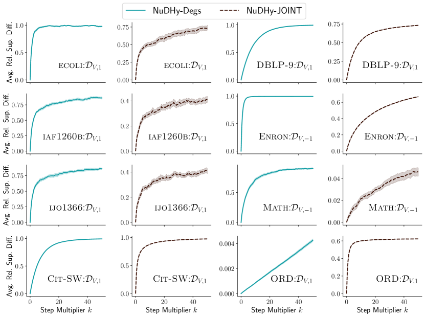
Figure 7: Convergence experiment for each dataset, for NuDHy-Degs and NuDHy-JOINT.

We note that although NuDHy-Degs-MH and NuDHy-JOINT-MH (not shown in the charts) require fewer steps to reach convergence due to their acceptance probability mechanism, which prioritizes visiting dense regions more frequently and sparse regions less often, their overall speed is hindered by the need to compute the degree of a state, which has a time complexity of $O(|V|^{2})$. This computation adds a significant overhead, and as a result, the time saved by performing fewer steps is counterbalanced by the increased complexity of the step operations. Consequently, NuDHy-Degs-MH ends up being slower than NuDHy-Degs, and NuDHy-JOINT-MH slower than NuDHy-JOINT. As an example, to perform the same amount of steps, for the small datasets (ecoli, iaf1260b, ijo1366), we report a time increase for NuDHy-Degs-MH from $5.86$x to $13.49$x; whereas for the mid-size datasets (cit-sw, math, dblp-9, enron), it is from $23.59$x to $187.2$x.

Appendix G Extended Experimental Evaluation of NuDHy

In this section, we delve into the experimental evaluation of our framework, which considered various metrics either specifically designed or extended to accommodate the unique characteristics of directed hypergraphs. Our primary objective is to discern which samplers produce hypergraphs that closely mimic the structural patterns of the original hypergraph. Our second objective is to shed light on the factors influencing the observed characteristics and, in particular, understand whether the properties of the original hypergraph preserved by the random hypergraphs generated by the samplers are among such factors. To this aim, we compare the values of the metrics calculated in the original hypergraph against those derived from $33$ random hypergraphs generated by each sampler.

G.1 Higher-order Reciprocity

Reciprocity  (?) is a statistic originally defined for directed graphs, and later on extended to directed hypergraphs  (?). It quantifies how mutually nodes are linked and thus allows a better understanding of the organizing principles of the hypergraph. The reciprocity of a hyperedge $e$ is measured considering a set $R_{e}$ of hyperedges sharing vertices with $e$. Informally, if the head (resp. tail) of $e$ overlaps with the tails (resp. heads) of the hyperedges in $R_{e}$ to a greater extent, then it is more reciprocal. Given the hyperedge $e\doteq(h,t)$, let $p_{u}(v)$ denote the transition probability from a node $u\in h$ to each node $v$, i.e., the probability of a random walker transiting from $u$ to $v$ when she moves to a uniform random tail-node of a uniform random arc among the hyperedges in $R_{e}$. In addition, let $p_{u}^{*}$ be the optimal transition probability, i.e., the probability when $R_{e}=\{(t,h)\}$. Then, the reciprocity of $e$ in the directed hypergraph $H\doteq(V,E)$ is

$$\mathsf{r}(e,R_{e})\doteq\left(\frac{1}{|R_{e}|}\right)^{\alpha}\left(1-\frac{\sum_{u\in h}\mathcal{L}(p_{u},p_{u}^{*})}{|h|\mathcal{L}_{\mathrm{max}}}\right)\,,$$

where $\alpha\in(0,1]$ is a penalization term  for large sets $R_{e}$, $\mathcal{L}(p_{u},p_{u}^{*})$ is the Jensen-Shannon Divergence between the distributions $p_{u}$ and $p_{u}^{*}$, $\mathcal{L}_{\mathrm{max}}$ is the maximum value taken by $\mathcal{L}$, and

$$R_{e}\doteq\arg\max_{R\subseteq E}\mathsf{r}(e,R)\,.$$

Finally, the reciprocity of $H$ is simply the average reciprocity of its hyperedges:

$$\mathsf{r}(H)\doteq\frac{1}{|E|}\sum\limits_{e\in E}\mathsf{r}(e,R_{e})\,.$$ (45)

The goal of this analysis is to demonstrate the ability of NuDHy to produce random hypergraphs with realistic reciprocity patterns, even though reciprocity is not inherently enforced in their design. Additionally, we aim to showcase their efficiency by generating such hypergraphs in significantly less time compared to Base and BaseD.

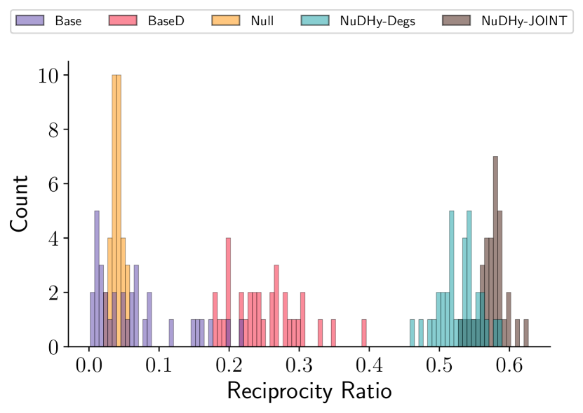
(a) ecoli

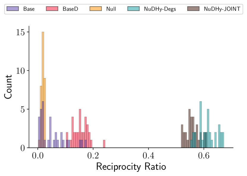
(b) iaf1260b

Figure 8: Distribution of the ratios between the reciprocity of $33$ samples and the observed reciprocity, for each sampler, for ecoli (left) and iaf1260b (right).

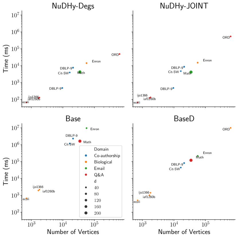
Figure 9: Mean time (ms) required to generate a sample using each of the samplers, for datasets of different size and different domain. Values are in log scale.

Figure 8 illustrates the distributions of reciprocity values obtained from $33$ samples generated by each sampler, where each value is divided by the reciprocity of the observed hypergraph. Across all cases, the mean reciprocity values of our samples closely approximate the observed reciprocity, outperforming the mean reciprocity values derived from the samples generated by our competitors. Specifically, the mean reciprocity among the samples generated by NuDHy-Degs range from 47% lower to 37% lower compared to the observed reciprocity. For NuDHy-JOINT, this range is from 33% to 18%. In contrast, Base and BaseD exhibit mean reciprocity values that deviate more significantly, with values from 95% to 93% for Base, and from 98% to 75% for BaseD. By looking at Figure 9, we can observe that our samplers efficiently complete the generation process in few seconds across most datasets. In contrast, Base and BaseD require at least one order of magnitude more time to terminate the generation, with Base being unable to complete the generation process within a 24-hour time frame for the largest datasets.

Similar mean reciprocity values among the various samplers are evident only in the case of enron, where NuDHy-Degs and Base lead to a mean reciprocity 50% lower than the observed reciprocity, whereas NuDHy-JOINT 35% lower. This particular case stands out from the others due to the unique characteristic of all heads having size 1. As a result, the fact that Base preserves the undirected group degrees (i.e., number of hyperedges that contain the group either in the head or in the tail) leads to samples that approximately maintain the directed group degrees (i.e, number of heads and number of tails that contain the group). Consequently, the samples generated by Base exhibit similar characteristics, on average, to those produced by NuDHy-Degs.

G.2 Node Centrality

As there are neither intuitive nor efficient measures of centrality specifically designed for directed hypergraphs, we measure the centrality of a node in a directed hypergraph, by first transforming the hypergraph into a graph, and then running two classic algorithms for node centrality in graphs: PageRank  (?) and HITS  (?). PageRank determines the importance of a node based on its link structure, so that a node is important if it is linked to by important nodes. HITS identifies two types of important nodes: hubs and authorities. Hubs are nodes connected to many relevant nodes; while authorities are nodes with many in-going edges from hubs. We run the PageRank algorithm on the directed weighted graph generated by creating a node for each node in the directed hypergraph and an edge from each node in a head of a hyperedge to each node in the tail of such hyperedge. The edge weight is the number of hyperedges in which the source node is in the head and the destination node is in the tail. On the other hand, we run the HITS algorithm on the directed bipartite graph representation of the directed hypergraph.

Table 6: Mean and standard deviation (in parentheses) of the Normalized Discounted Cumulative Gain (nDCG) of the rankings of the nodes obtained according to the Authority (Auth), Hub, and PageRank (Page) scores in $33$ samples, for each sampler.

	Score	Base	BaseD	Null	NuDHy-Degs	NuDHy-JOINT
ecoli	Auth	0.325 (0.081)	0.333 (0.074)	0.235 (0.030)	0.588 (0.311)	0.707 (0.370)
	Hub	0.326 (0202)	0.354 (0.185)	0.211 (0.018)	0.633 (0.357)	0.618 (0.357)
	Page	0.731 (0.053)	0.748 (0.041)	0.573 (0.021)	0.928 (0.012)	0.933 (0.009)
iaf1260b	Auth	0.346 (0.006)	0.380 (0.047)	0.347 (0.009)	0.558 (0.157)	0.588 (0.170)
	Hub	0.212 (0.011)	0.290 (0.054)	0.213 (0.023)	0.910 (0.225)	0.866 (0.282)
	Page	0.475 (0.006)	0.525 (0.024)	0.482 (0.009)	0.957 (0.005)	0.960 (0.003)
ijo1366	Auth	0.526 (0.012)	0.523 (0.008)	0.527 (0.013)	0.549 (0.023)	0.539 (0.022)
	Hub	0.385 (0.012)	0.374 (0.012)	0.395 (0.018)	0.380 (0.007)	0.380 (0.012)
	Page	0.465 (0.008)	0.462 (0.007)	0.472 (0.011)	0.959 (0.004)	0.960 (0.002)
cit-sw	Auth	0.695 (0.003)	0.708 (0.010)	0.694 (0.010)	0.735 (0.017)	0.739 (0.019)
	Hub	0.139 (0.035)	0.197 (0.073)	0.124 (0.004)	0.890 (0.246)	0.363 (0.010)
	Page	0.835 (0.002)	0.849 (0.001)	0.826 (0.002)	0.972 (0.001)	0.979 (0.001)
math	Auth	0.220 (0.015)	0.208 (0.004)	0.206 (0.005)	0.983 (0.001)	0.987 (0.001)
	Hub	0.213 (0.036)	0.195 (0.008)	0.194 (0.007)	0.451 (0.213)	0.410 (0.178)
	Page	0.609 (0.080)	0.572 (0.002)	0.569 (0.002)	0.974 (0.003)	0.977 (0.001)
dblp-9	Auth	0.338 (0.066)	0.345 (0.027)	0.311 (0.004)	0.567 (0.188)	0.538 (0.158)
	Hub	0.211 (0.018)	0.278 (0.074)	0.196 (0.004)	0.582 (0.122)	0.920 (0.233)
	Page	0.738 (0.005)	0.770 (0.004)	0.696 (0.003)	0.959 (0.001)	0.967 (0.001)
enron	Auth	0.285 (0.015)	0.397 (0.012)	0.263 (0.004)	0.798 (0.001)	0.982 (0.000)
	Hub	0.180 (0.017)	0.183 (0.029)	0.156 (0.006)	0.485 (0.214)	0.498 (0.197)
	Page	0.792 (0.002)	0.820 (0.002)	0.779 (0.001)	0.934 (0.002)	0.979 (0.001)
ord	Auth	$-$	0.803 (0.003)	0.802 (0.000)	0.813 (0.008)	0.815 (0.009)
	Hub	$-$	0.502 (0.061)	0.178 (0.002)	0.998 (0.000)	0.992 (0.000)
	Page	$-$	0.905 (0.003)	0.903 (0.000)	0.983 (0.000)	0.982 (0.000)

In this experiment we investigate whether node centrality is solely determined by node degrees or if natural patterns of node connections give rise to hubs and authorities. To assess this, we conducted the HITS and PageRank algorithms on each sample (as explained above), calculating the average scores for each node across all samples. We then evaluated the rankings generated by each score in terms of normalized Discounted Cumulative Gain (nDCG). nDCG  (?) is a metric used in information retrieval to evaluate the quality of rankings. It quantifies how well a ranking aligns with the relevance of its items, under the assumption that highly relevant items should appear earlier in the list. nDCG computes a gain for each item based on its relevance and discounts this gain as items appear lower in the ranking. The gains are accumulated to form a cumulative gain, which is then normalized by the ideal cumulative gain, representing a perfect ranking. In our experiments, we use the ranking from the observed hypergraph as measure of node relevance.

The results for each dataset and sampler are presented in Table 6. We note that the PageRank score is influenced by the number of incoming links to a node. While NuDHy-Degs maintains the frequency of a node appearing in heads or tails, it does not preserve the frequency of appearance in heads/tails of specific sizes. Consequently, it does not fully preserve node degrees in the graph projection used for PageRank. Nevertheless, we observe high nDCG scores, indicating that relative node importance is preserved. NuDHy-JOINT, which maintains the frequency of a node of a certain degree appearing in heads/tails of specific sizes, achieves slightly higher scores than NuDHy-Degs, due to its preservation of node degrees in the graph projection. In the case of Base and BaseD, which preserve head and tail sizes only on average, there is greater variability in the PageRank scores, resulting in lower nDCG scores. This is particularly noticeable for Base, which preserves node degrees on average, whereas BaseD preserves group degrees.

For Authority and Hub scores, we generally observe moderate to high nDCG scores. The exceptions occur in datasets where there are either no authorities or no hubs (i.e., scores are nearly 0 for all nodes). In such cases, clear node rankings are absent, rendering the nDCG less meaningful. For instance, in iaf1260b, ijo1366, and ecoli, more than half of the nodes have an authority score of 0, while other nodes have scores close to 0. In math, hub scores are almost always 0.

The fact that we do not observe perfect nDCG scores for rankings based on Hub and Authority scores suggests that having a high number of outgoing links does not necessarily make a node a hub, nor does having a large number of incoming links make a node an authority. Instead, it underscores the significance of the actual connections between nodes in determining hub and authority status.

G.3 Hyper-coreness Distribution

The $k$-core decomposition is a powerful method for analyzing the structure of (hyper)graphs by dividing them into increasingly connected components. This hierarchical decomposition provides a fingerprint of the (hyper)graph’s organization, which is essential for various applications such as modeling spreading processes and quantifying influence  (?). In fact, the coreness of a node, defined as the highest $k$ for which the node belong to the $k$-core, can measure its centrality and determine the potential impact of initiating a spreading process from that node. In the case of undirected hypergraphs, the core decomposition problem aims to identify a hierarchy of $(k,m)$-hyper-cores  (?). These hyper-cores are maximal sub-hypergraphs where each node is part of at least $k$ hyperedges with size at least $m$ within the hyper-core itself. Then, the m-shell index $c_{m}(v)$ of a node $v$ is the value $k$ at which $v$ belongs to the $(k,m)$-hyper-core but not to the $(k+1,m)$-hyper-core. Finally, the concept of hyper-coreness, denoted as $\mathsf{HC}$, provides a comprehensive measure of a node’s centrality by considering multiple $m$-shell indices:

$$\mathsf{HC}(v)=\sum\limits_{m=2}^{M}\omega(m)c_{m}(v)/k_{m}^{\mathrm{max}}\,,$$

where $k_{m}^{\mathrm{max}}$ is the maximum $k$ such that there exists at least one node with $m$-shell index $k$, and $\omega(m)$ is a function to account for the significance of the different sizes of higher-order interactions .

We extend this decomposition to directed hypergraph, by defining the $(k,m)$-h-hyper-core $C^{\textsc{h}}_{k,m}$ (resp. the $(k,m)$-t-hyper-core $C^{\textsc{t}}_{k,m}$) as the maximal sub-hypergraph where each node belongs to at least $k$ heads (resp. $k$ tails) of hyperedges of size $m$, within the h-hyper-core (resp. t-hyper-core) itself. Then, we define the $m$-h-shell index $c_{m}^{\textsc{h}}(v)$ and the $m$-t-shell index $c_{m}^{\textsc{t}}(v)$ of a node $v$ as  (?)

$$c_{m}^{\textsc{h}}(v) =\max_{k}\left\{k\mathrel{:}v\in C^{\textsc{h}}_{k,m}\right\}$$ (46)

$$c_{m}^{\textsc{t}}(v) =\max_{k}\left\{k\mathrel{:}v\in C^{\textsc{t}}_{k,m}\right\}$$ (47)

and the h-hyper-coreness and t-hyper-coreness of $v$ as the weighted sum of the shell indices:

$$\mathsf{HC}^{\textsc{h}}(v) =\sum\limits_{m=2}^{M}\omega(m)c_{m}^{\textsc{h}}(v)/k_{m}^{\textsc{h}}$$ (48)

$$\mathsf{HC}^{\textsc{t}}(v) =\sum\limits_{m=2}^{M}\omega(m)c_{m}^{\textsc{t}}(v)/k_{m}^{\textsc{t}}$$ (49)

where $k_{m}^{\textsc{h}}$ (resp. $k_{m}^{\textsc{t}}$) is the max value $k$ for which $C^{\textsc{h}}_{k,m}\neq\varnothing$ (resp. $C^{\textsc{t}}_{k,m}\neq\varnothing$).

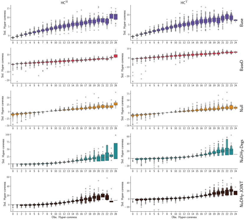
Figure 10: dblp-9: Distribution of the standardized $\mathsf{HC}^{\textsc{h}}$ (left) and $\mathsf{HC}^{\textsc{t}}$ scores, for each value measured in the observed hypergraph, for each sampler.

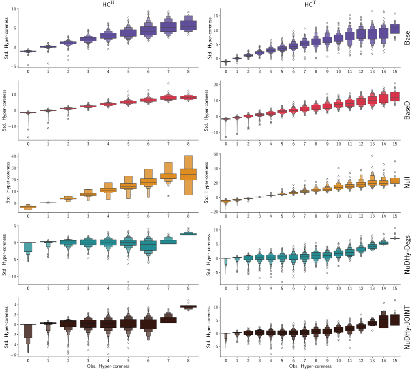
Figure 11: math: Distribution of the standardized $\mathsf{HC}^{\textsc{h}}$ (left) and $\mathsf{HC}^{\textsc{t}}$ scores, for each value measured in the observed hypergraph, for each sampler.

Figure 10 and Figure 11 illustrate the distribution of standardized $\mathsf{HC}^{\textsc{h}}$ (left) and $\mathsf{HC}^{\textsc{t}}$ (right) scores, for each sampler. To obtain these scores, we took the observed score of a node, subtract its mean score in the samples, and divide by its standard deviation. In general, we find that scores tend to deviate further from $0$ for nodes with stronger connections. This outcome aligns with our expectations because nodes with low hyper-coreness are typically associated with low degrees, and by shuffling the connections of low-degree nodes, it is not possible to significantly boost their hyper-coreness. Conversely, connecting nodes with high degrees to nodes with low degrees can diminish the hyper-coreness of the former. Given that BaseD preserves, on average, the appearances of node groups, it also tends to maintain the neighborhood of each node. Consequently, a well-connected node in the observed hypergraph typically corresponds to a densely-connected node in a sample. This results in similar average hyper-coreness values and standardized scores that are close to $0$. On the other hand, Null does not preserve the degrees of the nodes, leading to scenarios in which nodes that are sparsely-connected in the observed hypergraph become densely-connected in the samples. This can result in negative standardized scores. Finally, by considering the samples generated by NuDHy-Degs, we can identify relevant nodes with hyper-coreness higher than random. In dblp-9, these nodes can correspond to authors who cite/are cited by many authors that, in turn, cite/are cited by numerous other authors. This suggests a tendency for papers to reference similar groups of co-cited authors. This pattern is less pronounced when NuDHy-JOINT is employed, as it maintains the degrees of the neighbors of each node.

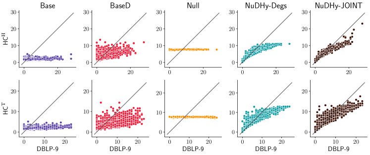
(a) dblp-9

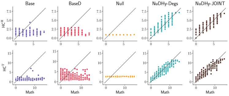
(b) math

Figure 12: Scatterplot of $\mathsf{HC}^{\textsc{h}}$ (top) and $\mathsf{HC}^{\textsc{t}}$ (bottom) scores measured in the observed hypergraph (x-axis) and averages in $33$ samples (y-axis), for each sampler.

Figure 12 compares the observed $\mathsf{HC}^{\textsc{h}}$ (top) and $\mathsf{HC}^{\textsc{t}}$ (bottom) scores with the mean scores in the samples, for each sampler. We observe a distinct trend for NuDHy-Degs and NuDHy-JOINT. The distribution of mean scores for NuDHy-JOINT more closely follows the distribution of observed scores, while the mean scores for NuDHy-Degs tend to be higher for nodes with low observed scores and lower for nodes with high observed scores. This suggests that NuDHy-Degs disrupts higher-order relations more than NuDHy-JOINT does. Since Null populates the hyperedges with nodes chosen uniformly at random, it leads to similar hyper-coreness values for all nodes. Finally, Base and BaseD may generate a different number of hyperedges and, on average, maintain the degree distributions but not the degree sequences. Consequently, nodes with high degrees in the observed hypergraph may exhibit low degrees in the samples, and vice versa. This explains the consistent wide range of mean hyper-coreness values for each observed hyper-coreness value.

Table 7: Mean and standard deviation (in parentheses) of the Normalized Discounted Cumulative Gain (nDCG) of the rankings of the vertices obtained according to the h-hyper-coreness and the t-hyper-coreness in $33$ samples, for each dataset and each sampler. To ensure a fair comparison, we did not normalize the values by $k_{m}^{\textsc{h}}$ and $k_{m}^{\textsc{t}}$ as in Equation 48.

	Base		BaseD		Null		NuDHy-Degs		NuDHy-JOINT
	$\mathsf{HC}^{\textsc{h}}$	$\mathsf{HC}^{\textsc{t}}$	$\mathsf{HC}^{\textsc{h}}$	$\mathsf{HC}^{\textsc{t}}$	$\mathsf{HC}^{\textsc{h}}$	$\mathsf{HC}^{\textsc{t}}$	$\mathsf{HC}^{\textsc{h}}$	$\mathsf{HC}^{\textsc{t}}$	$\mathsf{HC}^{\textsc{h}}$	$\mathsf{HC}^{\textsc{t}}$
ecoli	0.844	0.786	0.873	0.815	0.809	0.743	0.969	0.944	0.970	0.949
	(0.014)	(0.023)	(0.012)	(0.018)	(0.010)	(0.008)	(0.006)	(0.013)	(0.005)	(0.018)
iaf1260b	0.821	0.867	0.842	0.877	0.829	0.870	0.974	0.978	0.973	0.980
	(0.006)	(0.004)	(0.005)	(0.005)	(0.005)	(0.003)	(0.003)	(0.003)	(0.002)	(0.002)
ijo1366	0.837	0.872	0.851	0.869	0.833	0.872	0.976	0.980	0.976	0.982
	(0.005)	(0.004)	(0.002)	(0.003)	(0.005)	(0.003)	(0.002)	(0.002)	(0.003)	(0.002)
cit-sw	0.857	0.887	0.892	0.907	0.841	0.875	0.984	0.984	0.987	0.986
	(0.003)	(0.002)	(0.002)	(0.001)	(0.002)	(0.001)	(0.001)	(0.001)	(0.001)	(0.001)
math	0.872	0.798	0.863	0.764	0.862	0.763	0.986	0.987	0.986	0.988
	(0.001)	(0.002)	(0.001)	(0.001)	(0.001)	(0.002)	(0.001)	(0.001)	(0.001)	(0.001)
dblp-9	0.857	0.848	0.898	0.892	0.838	0.832	0.984	0.984	0.993	0.986
	(0.002)	(0.002)	(0.002)	(0.001)	(0.001)	(0.002)	(0.001)	(0.001)	(0.000)	(0.000)
enron	0.773	0.822	0.789	0.899	0.732	0.796	0.973	0.987	0.971	0.988
	(0.004)	(0.002)	(0.005)	(0.001)	(0.003)	(0.002)	(0.001)	(0.001)	(0.001)	(0.001)
ord	$-$	$-$	0.915	0.952	0.886	0.951	0.992	0.986	0.994	0.988
	$-$	$-$	(0.000)	(0.000)	(0.001)	(0.000)	(0.000)	(0.000)	(0.000)	(0.000)

While variations exist in the individual hyper-coreness values, Table 7 reveals that the Normalized Discounted Cumulative Gain (nDCG) for ranking the vertices based on mean scores compared to the rankings derived from the observed scores is consistently high across all samplers. In particular, both NuDHy-Degs and NuDHy-JOINT exhibit nearly perfect scores, signifying their ability to uphold the positions of the top-ranked nodes. In contrast, Null generally yields the lowest gains in nDCG, primarily due to the preservation of a smaller number of properties from the observed hypergraph.

G.4 Structural Entropy

We capture the probabilistic structure of a hypergraph $H$ at different granularity levels, by measuring the probability that a set of nodes of a certain size that is in the head (resp. tail) of some hyperedge in $H$ is also found in the head (resp. tail) of a hyperedge in a randomly sampled hypergraph from our null models DHCM and DHJM. The following approach is adapted from  (?). For each $j\in\{1,2\}$, this probability can be expressed as follows:

$$\mathbb{P}(S|\mathcal{Z}_{j})=\frac{1}{n}\sum_{i=1}^{n}X_{S}(H_{i})\,,$$

where each $H_{i}$ is a hypergraph sampled from $\mathcal{Z}_{j}$, and $X_{S}(H_{i})$ takes value $1$ if the set of nodes $S$ appears in the head (resp. tail) of a hyperedge in $H_{i}$, and $0$ otherwise. To quantify the entropy of these probabilities, denoted as $\hat{p}$, we use the following expression:

$$S(\hat{p})=-\hat{p}\log(\hat{p})-(1-\hat{p})\log(1-\hat{p})\,.$$ (50)

This measure quantifies the variability of the hyperedges across the sampled hypergraphs, as it grows as $\hat{p}$ moves away from the extreme values $0$ (the node group appears in no sample) and $1$ (the node group appears in each sample).

Figure 13: dblp-9: entropy of the head and tail node group probabilities, for groups of size $k=2$ and $k=3$, for each sampler.

To assess the degree of randomness in real-world hypergraph interaction processes, we investigate the likelihood that groups of nodes, engaging in interactions within the observed hypergraph (either in heads or tails), also participate in similar interactions within samples generated by the various samplers. Figure 13 shows the distribution of entropy values for these probabilities (Equation 50), for groups of sizes $k=2$ and $k=3$ in the heads (only for dblp-9) and in the tails. We define a certainty threshold at $0.1$ (i.e, 10% of the samples) and classify as uncertain all the groups with entropy greater than $S(0.1)\approxeq 0.469$ (green dotted line in the plots). As we can see, the majority of groups exhibit a high degree of certainty (i.e., they are either almost always present or absent in the samples), especially in the tails. This lower uncertainty may be attributed to the fact that, in most samples and for various group sizes, the probability of observing a specific group in the tail is close to zero, resulting in low entropy values. This trend is particularly prominent for the samples generated by Base and BaseD, because they struggle to accurately preserve the appearance of larger-sized groups.

Figure 14 further highlights that associations involving larger group sizes are disrupted by the samplers. This figure shows the empirical cumulative distribution (ECDF) of the head node group probabilities, for groups of size $k=2$ (left charts) and $k=3$ (right charts), for ecoli and ord. Null does not preserve any group of size $3$ and preserves the lowest amount of groups of size $2$. Base follows a similar behavior, achieving slightly higher node group probabilities in the heads. Among the competitors, BaseD is the most performing, as it preserves, on average, the number of appearances of each node group in the samples. Finally, NuDHy-JOINT is the only sampler able to generate random hypergraphs preserving the appearance of groups of size $3$ with high probability. The fact that NuDHy-Degs struggles to preserve such appearances indicates the presence of a preference mechanism underlying the network, rather than these associations being mere consequences of node degrees.

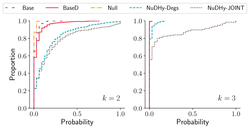
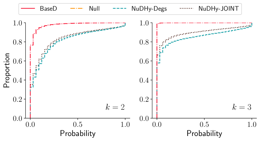
Figure 14: ECDF of the heads node group probabilities, for groups of size $k=2$ (left chart) and $k=3$ (right chart), for each sampler, for ecoli (left figure) and ord (right figure).

G.5 Multi-order Spectrum

Let $\hat{H}=(V,U)$ be the undirected hypergraph obtained by merging the head and tail of each directed hyperedge in the directed hypergraph $H\doteq(V,E)$. The generalized Laplacian of order $d$ of $\hat{H}$ is $L^{(d)}\doteq dK^{(d)}-A^{(d)}$, where $K^{(d)}$ is the degree matrix of order $d$, i.e., a diagonal matrix where each entry $K^{(d)}[v,v]$ indicates the number of hyperedges in $U$ of dimension $d$ including $v$; and $A^{(d)}$ is a symmetric matrix indicating, for each $(u,v)$, the number of hyperedges in $U$ of size $d$ containing both $u$ and $v$. The multi-order Laplacian of $\hat{H}$  (?) is defined as the weighted sum of the Laplacian matrices of order $d$, i.e.,

$$L^{(\mathrm{mul})}\doteq\sum_{d=2}^{D}\frac{\omega(d)}{\langle K^{(d)}\rangle}L^{(d)}\,,$$

where $\omega(d)$ is a function to account for the significance of the different orders, $\langle K^{(d)}\rangle$ indicates the average degree of order $d$, and $D\in[1,|V|]$. The spectrum of $L^{(\mathrm{mul})}$ is the list of its eigenvalues $\Lambda=[\Lambda_{1},\ldots,\Lambda_{n}]$, sorted in descending order. We note that in this analysis, we do not consider the Laplacian matrix of the directed hypergraph $H$ as, in general, it is not symmetric, and thus, the eigenvalues may not be all real numbers.

The spectrum plays an important role in (hyper)network analysis, as it reveals information about the connectivity and robustness of the corresponding hyper(graph). Similarity between two spectra implies similarity in structural properties and connectivity of the corresponding hypergraphs.

Given two hypergraphs $H_{1}$ and $H_{2}$, we extracted their top-$k$ smallest eigenvalues $\Lambda^{1,k}$ and $\Lambda^{2,k}$ and measured the spectral distance between $H_{1}$ and $H_{2}$ as follows  (?, ?):

$$\mathsf{sd}(H_{1},H_{2})\doteq\frac{1}{k}||\Lambda^{1,k}-\Lambda^{2,k}||_{2}\,.$$

Low distance values indicate that the two hypergraphs are structurally similar, i.e., they are characterized by similar structural patters, local connectivity, and community structure.

We limited our analysis to the top-$6$ eigenvalues due to the computational complexity of the eigen-decomposition process, and we set $D$ equal to the minimum between the $8$ and the maximum dimension of a hyperedge in the original hypergraph.

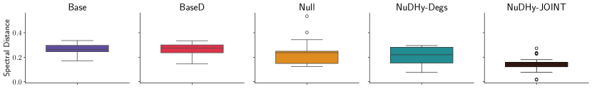
(a) ecoli

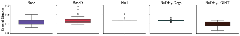
(b) ijo1366

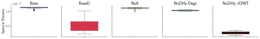
(c) enron

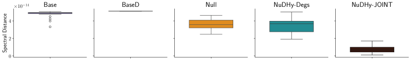
(d) math

Figure 15: Distribution of the spectral distances between the spectrum of the observed hypergraph and that of $33$ samples, for each sampler, for ecoli, ijo1366, enron, and math.

Figure 15 shows the distribution of spectral distances across $33$ samples for each sampler, for four datasets. We observe that NuDHy-JOINT consistently exhibit stable performance across all datasets, resulting in smaller distances between the eigenvalue vectors of the multi-order Laplacian, compared to those observed for Base, BaseD, and Null. On the other hand, NuDHy-Degs often achieves distances comparable to those measured for the samples generated by Null, indicating that the degree distribution alone does not preserve the community structure of the original hypergraph.

Interestingly, BaseD, which maintains node degrees on average, produces samples exhibiting spectral distance from the original hypergraph more akin to that observed in samples generated by Base (which preserves group degrees), rather than those generated by NuDHy-Degs, despite NuDHy-Degs exactly preserving the same properties. This difference may be attributed to the constraint imposed by the design of Base and BaseD, limiting the size of each hyperedge to $10$.

G.6 Party Homophily in the US Congress

Figure 16 shows the extent to which Republicans’ and Democrats’ observed homophily exceeds what would be expected if co-sponsoring relations formed randomly among legislators. Consistently with prior research  (?), we observe that both parties exhibit an inclination toward associating with similar party members in co-sponsorship relations. Then, we note that the inverse relationship between the curves of Republicans and Democrats, akin to the affinity plots, remains discernible, a pattern that remains unnoticed when solely examining the values of $\mathsf{m}$ measured in the observed hypergraphs.

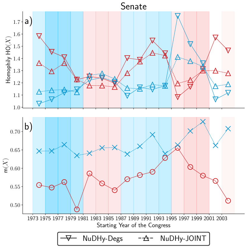
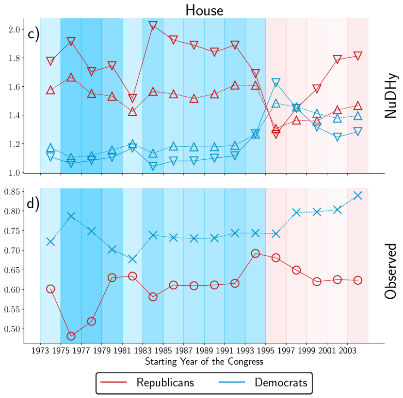
Figure 16: Homophily in the US Congress co-sponsored bills. We show results for Equation 5 using $33$ samples generated by NuDHy-Degs and NuDHy-JOINT for the US Senate (S-bills), panel (a)) and House (H-bills), panel (c)). For comparison, we show the values of $\mathsf{m}(X)$ again for the US Senate (panel (b)) and House (panel (d)). The colors indicate Democrats (blue) and Republicans (red).

G.7 Econometric Competitiveness: Analysis for Other Trade Networks

Table 8 reports the mean Spearman’s correlation and Kendall’s Tau of the rankings of the countries obtained according to the GENEPY/ECI scores in $33$ samples generated by each sampler with respect to the rankings obtained from the observed GENEPY/ECI scores, for hs1995, hs2009,and hs2020. The performances of the samplers are consistent through the various years, with NuDHy-Degs and NuDHy-JOINT achieving the most correlated rankings with respect to the GENEPY scores. Regarding ECI, only NuDHy-JOINT leads to rankings that resemble that obtained from the observed scores.

Table 8: Mean Spearman’s correlation and Kendall’s Tau (KT) of the rankings of the countries obtained according to the ECI/Fitness/GENEPY scores in $33$ samples with respect to the rankings obtained from the observed scores. Standard deviations are reported in parentheses.

Score	Metric	Year	Base	BaseD	Null	NuDHy-Degs	NuDHy-JOINT
ECI	Spearman	1995	-0.183 (0.143)	-0.062 (0.118)	0.011 (0.071)	0.031 (0.112)	0.947 (0.004)
		2009	-0.251 (0.143)	-0.110 (0.096)	-0.008 (0.079)	0.009 (0.094)	0.953 (0.002)
		2020	-0.223 (0.161)	-0.070 (0.135)	0.004 (0.102)	0.009 (0.121)	0.978 (0.001)
	KT	1995	-0.119 (0.094)	-0.042 (0.079)	0.008 (0.047)	0.022 (0.076)	0.817 (0.005)
		2009	-0.167 (0.097)	-0.074 (0.064)	-0.005 (0.054)	-0.007 (0.065)	0.817 (0.006)
		2020	-0.152 (0.109)	-0.047 (0.090)	0.003 (0.068)	0.005 (0.082)	0.878 (0.004)
Fitness	Spearman	1995	0.162 (0.093)	0.314 (0.057)	-0.001 (0.082)	0.981 (0.001)	0.997 (0.000)
		2009	0.117 (0.086)	0.272 (0.051)	0.036 (0.076)	0.979 (0.001)	0.999 (0.000)
		2020	0.137 (0.082)	0.360 (0.054)	0.020 (0.097)	0.977 (0.001)	0.998 (0.000)
	KT	1995	0.110 (0.062)	0.215 (0.042)	0.000 (0.054)	0.882 (0.004)	0.962 (0.002)
		2009	0.078 (0.059)	0.182 (0.036)	0.025 (0.050)	0.884 (0.003)	0.963 (0.001)
		2020	0.091 (0.056)	0.245 (0.037)	0.014 (0.066)	0.881 (0.003)	0.964 (0.001)
GENEPY	Spearman	1995	0.110 (0.101)	0.312 (0.057)	0.002 (0.100)	0.953 (0.005)	0.995 (0.000)
		2009	0.083 (0.083)	0.264 (0.050)	0.034 (0.088)	0.931 (0.004)	0.994 (0.000)
		2020	0.099 (0.078)	0.348 (0.054)	0.007 (0.097)	0.941 (0.004)	0.994 (0.000)
	KT	1995	0.074 (0.069)	0.215 (0.041)	0.002 (0.067)	0.819 (0.009)	0.944 (0.002)
		2009	0.057 (0.056)	0.178 (0.036)	0.023 (0.060)	0.790 (0.007)	0.941 (0.002)
		2020	0.065 (0.053)	0.237 (0.038)	0.004 (0.064)	0.808 (0.007)	0.942 (0.002)

Figures 17, 18 and 19 illustrate the distribution of the rankings based on ECI/Fitness/GENEPY values across $33$ samples for NuDHy-Degs (left) and NuDHy-JOINT (right) in comparison to the observed rankings for hs1995, hs2009, and hs2020. In all cases, for NuDHy-JOINT, the distribution of rankings based on GENEPY closely mirrors the observed ranking, with noticeable deviations for the countries positioned in the middle of the observed ranking. Conversely, for NuDHy-Degs, deviations are more pronounced in the first positions of the rankings, but the overall trend aligns with the observed ranking.

Examining the rankings according to ECI reveals a different pattern. NuDHy-JOINT consistently produces distributions that closely align with the observed rankings. In contrast, NuDHy-Degs generates diverse ranks for countries, resulting in mean rankings significantly different from the observed ones.

These findings suggest that the joint degree distribution significantly affects the relative GENEPY scores, whereas other underlying patterns in the data contribute to the relative ECI scores. The degree distributions, which are weaker constraints than the joint distribution, fail to capture either the relative GENEPY or the relative ECI score distributions.

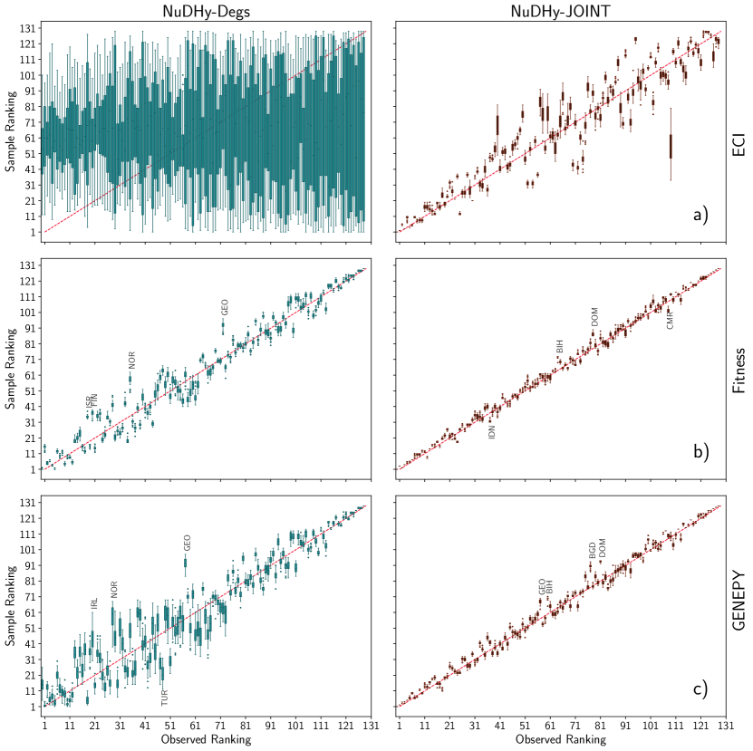
Figure 17: hs1995: Distributions of rankings obtained according to the ECI/Fitness/GENEPY values in $33$ samples for NuDHy-Degs (left) and NuDHy-JOINT (right) compared to the observed rankings. The top 4 countries whose observed rank diverges the most from the sample mean ranking are annotated in a subset of the plots.

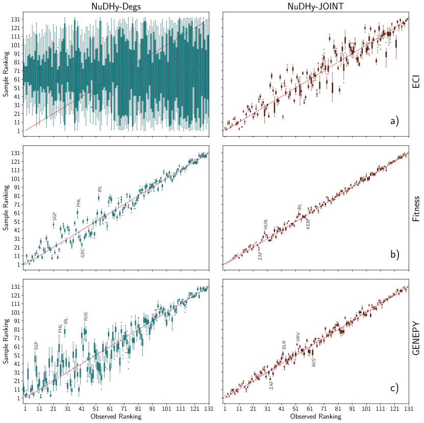
Figure 18: hs2009: Distributions of rankings obtained according to the ECI/Fitness/GENEPY values in $33$ samples for NuDHy-Degs (left) and NuDHy-JOINT (right) compared to the observed rankings. The top 4 countries whose observed rank diverges the most from the sample mean ranking are annotated in a subset of the plots.

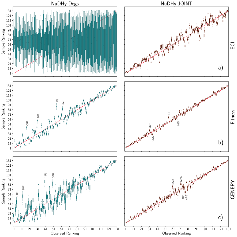
Figure 19: hs2020: Distributions of rankings obtained according to the ECI/Fitness/GENEPY values in $33$ samples for NuDHy-Degs (left) and NuDHy-JOINT (right) compared to the observed rankings. The top 4 countries whose observed rank diverges the most from the sample mean ranking are annotated in a subset of the plots.

References

- 1. F. Battiston, et al., Networks beyond pairwise interactions: Structure and dynamics, Phys. Rep. 874, 1–92 (2020).
- 2. F. Battiston, et al., The physics of higher-order interactions in complex systems, Nat. Phys. 17, 1093–1098 (2021).
- 3. C. Bick, E. Gross, H. A. Harrington, M. T. Schaub, What are higher-order networks?, SIAM Review 65, 686–731 (2023).
- 4. A. Ritz, B. Avent, T. Murali, Pathway analysis with signaling hypergraphs, TCBB 14, 1042–1055 (2015).
- 5. S. Feng, et al., Hypergraph models of biological networks to identify genes critical to pathogenic viral response, BMC bioinformatics 22, 1–21 (2021).
- 6. E. Schneidman, S. Still, M. J. Berry, W. Bialek, et al., Network information and connected correlations, Phys. Rev. Lett. 91, 238701 (2003).
- 7. E. Schneidman, M. J. Berry II, R. Segev, W. Bialek, Weak pairwise correlations imply strongly correlated network states in a neural population, Nature 440, 1007 (2006).
- 8. C. Giusti, E. Pastalkova, C. Curto, V. Itskov, Clique topology reveals intrinsic geometric structure in neural correlations, Proc. Natl. Acad. Sci. U.S.A. 112, 13455–13460 (2015).
- 9. G. Petri, et al., Homological scaffolds of brain functional networks, J. R. Soc. Interface 11, 20140873 (2014).
- 10. A. Patania, G. Petri, F. Vaccarino, The shape of collaborations, EPJ Data Sci. 6, 18 (2017).
- 11. Q. Luo, et al., Toward maintenance of hypercores in large-scale dynamic hypergraphs, VLDBJ pp. 1–18 (2022).
- 12. J. C. W. Billings, et al., Simplex2vec embeddings for community detection in simplicial complexes, arXiv preprint arXiv:1906.09068 (2019).
- 13. X. Luo, J. Peng, J. Liang, Directed hypergraph attention network for traffic forecasting, IET Intelligent Transport Systems 16, 85–98 (2022).
- 14. S. Ranshous, et al., Financial Cryptography and Data Security (2017), pp. 248–263.
- 15. K. Berlt, et al., Modeling the web as a hypergraph to compute page reputation, Information Systems 35, 530–543 (2010).
- 16. R. A. Fisher, Design of experiments, British Medical Journal 1, 554 (1936).
- 17. B. F. Manly, A note on the analysis of species co-occurrences, Ecology 76, 1109–1115 (1995).
- 18. T. Squartini, R. Mastrandrea, D. Garlaschelli, Unbiased sampling of network ensembles, New Journal of Physics 17, 023052 (2015).
- 19. W. E. Schlauch, K. A. Zweig, Proceedings of the 2015 IEEE/ACM International Conference on Advances in Social Networks Analysis and Mining 2015 (2015), pp. 514–519.
- 20. R. Fischer, J. C. Leitao, T. P. Peixoto, E. G. Altmann, Sampling motif-constrained ensembles of networks, Physical review letters 115, 188701 (2015).
- 21. N. D. Verhelst, An efficient mcmc algorithm to sample binary matrices with fixed marginals, Psychometrika 73, 705–728 (2008).
- 22. G. Strona, D. Nappo, F. Boccacci, S. Fattorini, J. San-Miguel-Ayanz, A fast and unbiased procedure to randomize ecological binary matrices with fixed row and column totals, Nature communications 5, 4114 (2014).
- 23. I. Stanton, A. Pinar, Constructing and sampling graphs with a prescribed joint degree distribution, Journal of Experimental Algorithmics 17, 3–1 (2012).
- 24. M. Gjoka, B. Tillman, A. Markopoulou, 2015 IEEE conference on computer communications (2015), pp. 1553–1561.
- 25. G. Cimini, et al., The statistical physics of real-world networks, Nature Reviews Physics 1, 58–71 (2019).
- 26. R. Kannan, P. Tetali, S. Vempala, Simple markov-chain algorithms for generating bipartite graphs and tournaments, Random Structures & Algorithms 14, 293–308 (1999).
- 27. L. Tabourier, C. Roth, J.-P. Cointet, Generating constrained random graphs using multiple edge switches, Journal of Experimental Algorithmics 16, 1–1 (2011).
- 28. F. Saracco, R. Di Clemente, A. Gabrielli, T. Squartini, Randomizing bipartite networks: the case of the world trade web, Scientific Reports 5, 10595 (2015).
- 29. A. A. Boroojeni, J. Dewar, T. Wu, J. M. Hyman, Generating bipartite networks with a prescribed joint degree distribution, Journal of complex networks 5, 839–857 (2017).
- 30. S. G. Aksoy, T. G. Kolda, A. Pinar, Measuring and modeling bipartite graphs with community structure, Journal of Complex Networks 5, 581–603 (2017).
- 31. C. I. Del Genio, H. Kim, Z. Toroczkai, K. E. Bassler, Efficient and exact sampling of simple graphs with given arbitrary degree sequence, PloS one 5, e10012 (2010).
- 32. F. Saracco, G. Petri, R. Lambiotte, T. Squartini, Entropy-based random models for hypergraphs, arXiv preprint arXiv:2207.12123 (2022).
- 33. M. T. Do, S.-e. Yoon, B. Hooi, K. Shin, SIGKDD (2020), pp. 176–186.
- 34. M. Barthelemy, Class of models for random hypergraphs, Physical Review E 106, 064310 (2022).
- 35. J.-L. Guo, X.-Y. Zhu, Q. Suo, J. Forrest, Non-uniform evolving hypergraphs and weighted evolving hypergraphs, Scientific Reports 6, 36648 (2016).
- 36. J.-W. Wang, L.-L. Rong, Q.-H. Deng, J.-Y. Zhang, Evolving hypernetwork model, The European Physical Journal B 77, 493–498 (2010).
- 37. P. S. Chodrow, Configuration models of random hypergraphs, Journal of Complex Networks 8, cnaa018 (2020).
- 38. Y. Zeng, B. Liu, F. Zhou, L. Lü, Hyper-null models and their applications, Entropy 25, 1390 (2023).
- 39. H. Sun, G. Bianconi, Higher-order percolation processes on multiplex hypergraphs, Physical Review E 104, 034306 (2021).
- 40. K. Nakajima, K. Shudo, N. Masuda, Randomizing hypergraphs preserving degree correlation and local clustering, IEEE Transactions on Network Science and Engineering 9, 1139–1153 (2021).
- 41. R. Miyashita, K. Nakajima, M. Fukuda, K. Shudo, IEEE International Conference on Big Data and Smart Computing (2023), pp. 316–317.
- 42. S. Kim, M. Choe, J. Yoo, K. Shin, ICDM (2022).
- 43. C. A. Hidalgo, B. Klinger, A.-L. Barabási, R. Hausmann, The product space conditions the development of nations, Science 317, 482–487 (2007).
- 44. A. Tacchella, M. Cristelli, G. Caldarelli, A. Gabrielli, L. Pietronero, A new metrics for countries’ fitness and products’ complexity, Scientific Reports 2 (2012).
- 45. C. Sciarra, G. Chiarotti, L. Ridolfi, F. Laio, Reconciling contrasting views on economic complexity, Nature communications 11, 3352 (2020).
- 46. J. Moody, Race, school integration, and friendship segregation in america, American journal of Sociology 107, 679–716 (2001).
- 47. C. P. Loomis, Political and occupational cleavages in a hanoverian village, germany: A sociometric study, Sociometry 9, 316–333 (1946).
- 48. P. F. Lazarsfeld, R. K. Merton, et al., Friendship as a social process: A substantive and methodological analysis, Freedom and control in modern society 18, 18–66 (1954).
- 49. M. McPherson, L. Smith-Lovin, J. M. Cook, Birds of a feather: Homophily in social networks, Annual review of sociology 27, 415–444 (2001).
- 50. N. Veldt, A. R. Benson, J. Kleinberg, Combinatorial characterizations and impossibilities for higher-order homophily, Science Advances 9, eabq3200 (2023).
- 51. J. H. Fowler, Legislative cosponsorship networks in the us house and senate, Social networks 28, 454–465 (2006).
- 52. J. Park, A.-L. Barabási, Distribution of node characteristics in complex networks, Proceedings of the National Academy of Sciences 104, 17916–17920 (2007).
- 53. M. Grossmann, D. A. Hopkins, Ideological republicans and group interest democrats: The asymmetry of american party politics, Perspectives on Politics 13, 119–139 (2015).
- 54. Z. P. Neal, R. Domagalski, X. Yan, Homophily in collaborations among us house representatives, 1981–2018, Social Networks 68, 97–106 (2022).
- 55. L. Peel, T. P. Peixoto, M. De Domenico, Statistical inference links data and theory in network science, Nature Communications 13, 6794 (2022). Number: 1 Publisher: Nature Publishing Group.
- 56. L. Röttjers, D. Vandeputte, J. Raes, K. Faust, Null-model-based network comparison reveals core associations, ISME Communications 1, 36 (2021).
- 57. B. Mønsted, P. Sapieżyński, E. Ferrara, S. Lehmann, Evidence of complex contagion of information in social media: An experiment using twitter bots, PloS one 12, e0184148 (2017).
- 58. M. Karsai, G. Iniguez, K. Kaski, J. Kertész, Complex contagion process in spreading of online innovation, Journal of The Royal Society Interface 11, 20140694 (2014).
- 59. I. Iacopini, G. Petri, A. Barrat, V. Latora, Simplicial models of social contagion, Nature communications 10, 2485 (2019).
- 60. G. F. de Arruda, G. Petri, Y. Moreno, Social contagion models on hypergraphs, Physical Review Research 2, 023032 (2020).
- 61. G. St-Onge, et al., Influential groups for seeding and sustaining nonlinear contagion in heterogeneous hypergraphs, Communications Physics 5, 25 (2022).
- 62. S. Cui, F. Liu, H. Jardón-Kojakhmetov, M. Cao, General sis diffusion process with indirect spreading pathways on a hypergraph, arXiv preprint arXiv:2306.00619 (2023).
- 63. G. St-Onge, H. Sun, A. Allard, L. Hébert-Dufresne, G. Bianconi, Universal nonlinear infection kernel from heterogeneous exposure on higher-order networks, Physical review letters 127, 158301 (2021).
- 64. D. T. Gillespie, Stochastic Simulation of Chemical Kinetics, Annual Review of Physical Chemistry 58, 35–55 (2007).
- 65. V. Gemmetto, A. Barrat, C. Cattuto, Mitigation of infectious disease at school: targeted class closure vs school closure, BMC infectious diseases 14, 1–10 (2014).
- 66. R. Mastrandrea, J. Fournet, A. Barrat, Contact patterns in a high school: a comparison between data collected using wearable sensors, contact diaries and friendship surveys, PloS one 10, e0136497 (2015).
- 67. A. R. Benson, R. Abebe, M. T. Schaub, A. Jadbabaie, J. Kleinberg, Simplicial closure and higher-order link prediction, Proceedings of the National Academy of Sciences 115, E11221–E11230 (2018).
- 68. M. M. de Oliveira, R. Dickman, How to simulate the quasistationary state, Phys. Rev. E 71, 016129 (2005).
- 69. A. Tacchella, M. Cristelli, G. Caldarelli, A. Gabrielli, L. Pietronero, Economic complexity: Conceptual grounding of a new metrics for global competitiveness, Journal of Economic Dynamics and Control 37, 1683–1691 (2013).
- 70. M. Cristelli, A. Gabrielli, A. Tacchella, G. Caldarelli, L. Pietronero, Measuring the intangibles: A metrics for the economic complexity of countries and products, PloS one 8, e70726 (2013).
- 71. B. Balassa, Trade liberalisation and “revealed” comparative advantage 1, The manchester school 33, 99–123 (1965).
- 72. H. G. Lab, Atlas complexity ranking. Https://atlas.cid.harvard.edu/rankings.
- 73. S. Inoua, A simple measure of economic complexity, Research Policy 52, 104793 (2023).
- 74. E. Pugliese, A. Zaccaria, L. Pietronero, On the convergence of the fitness-complexity algorithm, The European Physical Journal Special Topics 225, 1893–1911 (2016).
- 75. R. Hausmann, C. A. Hidalgo, S. Bustos, M. Coscia, A. Simoes, The atlas of economic complexity: Mapping paths to prosperity (Mit Press, 2014).
- 76. M. J. Straka, G. Caldarelli, T. Squartini, F. Saracco, From ecology to finance (and back?): A review on entropy-based null models for the analysis of bipartite networks, Journal of Statistical Physics 173, 1252–1285 (2018).
- 77. Y. Artzy-Randrup, L. Stone, Generating uniformly distributed random networks, Physical Review E 72, 056708 (2005).
- 78. A. S. S. Rao, C. R. Rao, Principles and methods for data science (Elsevier, 2020).
- 79. F. Viger, M. Latapy, Efficient and simple generation of random simple connected graphs with prescribed degree sequence, Journal of Complex Networks 4, 15–37 (2016).
- 80. É. Czabarka, A. Dutle, P. L. Erdős, I. Miklós, On realizations of a joint degree matrix, Discrete Applied Mathematics 181, 283–288 (2015).
- 81. H. J. Ryser, Combinatorial mathematics, vol. 14 (American Mathematical Soc., 1963).
- 82. A. Gionis, H. Mannila, T. Mielikäinen, P. Tsaparas, Assessing data mining results via swap randomization, TKDD 1, 14–es (2007).
- 83. P. R. Krugman, M. Obstfeld, International economics: Theory and policy (Pearson Education, 2009).
- 84. T. Shen, et al., A genome-scale metabolic network alignment method within a hypergraph-based framework using a rotational tensor-vector product, Scientific Reports 8, 1–16 (2018).
- 85. J. Tang, et al., ACM SIGKDD (2008), pp. 990–998.
- 86. S. M. Kearnes, et al., The open reaction database, Journal of the American Chemical Society 143, 18820–18826 (2021).
- 87. M. E. Newman, S. Forrest, J. Balthrop, Email networks and the spread of computer viruses, Physical Review E 66, 035101 (2002).
- 88. L. Tran, T. Quan, A. Mai, Pagerank algorithm for directed hypergraph, CoRR, abs/1909.01132 (2019).
- 89. J. M. Kleinberg, Authoritative sources in a hyperlinked environment, Journal of the ACM 46, 604–632 (1999).
- 90. K. Järvelin, J. Kekäläinen, Cumulated gain-based evaluation of ir techniques, ACM Transactions on Information Systems 20, 422–446 (2002).
- 91. D. Garcia, P. Mavrodiev, D. Casati, F. Schweitzer, Understanding popularity, reputation, and social influence in the twitter society, Policy & Internet 9, 343–364 (2017).
- 92. M. Mancastroppa, I. Iacopini, G. Petri, A. Barrat, Hyper-cores promote localization and efficient seeding in higher-order processes, arXiv preprint arXiv:2301.04235 (2023).
- 93. C. Giatsidis, D. M. Thilikos, M. Vazirgiannis, D-cores: measuring collaboration of directed graphs based on degeneracy, Knowledge and information systems 35, 311–343 (2013).
- 94. J.-G. Young, G. Petri, T. P. Peixoto, Hypergraph reconstruction from network data, Communications Physics 4, 135 (2021).
- 95. M. Lucas, G. Cencetti, F. Battiston, Multiorder laplacian for synchronization in higher-order networks, Physical Review Research 2, 033410 (2020).
- 96. I. Jovanović, Z. Stanić, Spectral distances of graphs, Linear algebra and its applications 436, 1425–1435 (2012).
- 97. J. Gu, B. Hua, S. Liu, Spectral distances on graphs, Discrete Applied Mathematics 190, 56–74 (2015).
[appendix] \printcontents[appendix]1