Semantic Information in MC: Chemotaxis Beyond Shannon

Abstract

The recently emerging molecular communication (MC) paradigm intents to leverage communication engineering tools for the design of synthetic chemical communication systems. These systems are envisioned to operate on nanoscale and in biological environments, such as the human body, and catalyze the emergence of revolutionary applications in the context of early disease monitoring and drug targeting. However, while a plethora of theoretical (and more recently also more and more practical) MC system designs have been proposed over the past years, some fundamental questions remain open, hindering the breakthrough of MC in real-world applications. One of these questions is: What is a useful measure of information in the context of MC-based applications? While most existing works in MC build upon the concept of syntactic information as introduced by Shannon, in this paper, we explore the framework of semantic information as introduced by Kolchinsky and Wolpert for the information theoretical analysis of a natural MC system, namely bacterial chemotaxis. Exploiting the computational modeling tool of agent-based modeling (ABM), we are able to demonstrate, for the first time, that the semantic information framework can provide a useful information theoretical framework for quantifying the information exchange of chemotactic bacteria with their environment. In particular, we show that the measured semantic information provides a useful measure of the ability of the bacteria to adapt to and survive in a changing environment, while, to the best of our knowledge, no comparable analysis exists in the context of syntactic information. Encouraged by our results, we envision that the semantic information framework can open new avenues for developing theoretical and practical MC system designs in the context of synthetic biology and in this way help to unleash the full potential of MC for complex adaptive systems-based nanoscale applications.

I Introduction

Transmission of information occurs at several levels of abstraction and, according to Weaver, can be categorized into the communication of (i) accurate syntactic information (technical level), (ii) the meaning/significance of a message (semantic level), and (iii) the actions caused by a message (effectiveness level) [1]. While unappreciated for a long time, the study of the semantic and effectiveness levels (the latter one also referred to as goal-oriented level) has recently received significant attention in the context of future sixth-generation (6G) communication networks, for example for communication in (among others) personalized body area networks, unmanned aerial vehicles-assisted networks, and networks of autonomous collaborative robots [2, 3, 4]. One particular benefit of studying communication on the semantic and effectiveness levels is the relevance of their respective performance metrics to the end-to-end performance of communication applications as compared to the metrics of the syntactic level. For example, the semantic metric age of information (AoI) is highly relevant for the design of efficient scheduling schemes in communication networks that rely on the timely delivery of information, e.g., for location tracking applications, while syntactic measures, such as the packet delay, are less relevant [3].

In this paper, we do not consider conventional communication systems based on electromagnetic waves, but the recently emerging MC systems; in these systems, information is transmitted by chemical messengers. Due to the physical nature of molecular transport, synthetic MC systems, according to experimental and theoretical studies, are characterized by relatively poor performance on the syntactic level (low achievable data rates, high bit error rates) compared to the extremely good performance observed on the effectiveness level in natural MC systems (e.g., complex adaptations of single-cell species to changing environmental conditions); this observation indicates that semantic information may be a highly relevant measure to consider in the analysis of MC systems. There is the possibility that a shift in perspective towards the analysis of semantic information and the underlying goal (effectiveness) may drive future synthetic MC systems and their applications, which are mainly centered around synthetic in-body communication for collaborative nanodevice-assisted early disease detection and targeted drug delivery [5]. Here, we explore this idea by developing a semantic information framework for bacterial chemotaxis, a widely considered MC system.

So far, there have been only a few attempts to create a useful information theoretic framework for MC that includes semantic communication [6, 7]. Both works are inspired by the framework of semantic information as introduced by Kolchinsky and Wolpert [8]. In [6], semantic information was proposed for the design of synthetic cells. However, the notion of semantic information considered in [6] does not quantify the dynamic information exchange between the synthetic cell and its environment and is, hence, limited in its generality. In [7], the concept of subjective information is introduced to measure how much useful information is obtained under different information acquisition strategies as compared to a default strategy. Here, the source of information is an environmental signal, and the useful information is defined as the mutual information between the subject’s actions and the environmental signal. However, the framework considered in [7] does not provide insight into the time-varying information exchange between subject and environment. Finally, the systems studied in [6] and [7] were developed in the context of the respective information theoretic analysis and have very limited complexity; hence, it is not clear to what extent they generalize to practical real-world systems.

In contrast to existing works, in this paper, we apply the generic framework proposed in [8] directly to the established computational run-and-tumble chemotaxis model from the literature; in this way we (i) demonstrate the applicability of the framework and (ii) ensure that the presented analysis is informed by real-world system observations. Furthermore, we extend previous works by considering and quantifying the dynamic adaptation of the considered chemotactic bacteria to their environment. Thus, the framework presented in this paper measures the dynamic transmission of semantic information in MC for the first time, considering chemotaxis as an exemplarily system. Finally, the obtained semantic information is related to the ability of the bacteria to adapt and survive in a changing environment, i.e., the effectiveness level of the considered MC system.

The remainder of this paper is organized as follows. In Section II, we describe the bacterial chemotaxis model. In Section III, we introduce the proposed semantic information theoretic framework and map it to our system model. In Section IV, we evaluate the framework. Finally, Section V concludes the paper and outlines topics for future work.

II System Model

II-A Bacterial Chemotaxis: Gradient-based Nutrient Detection

Bacterial chemotaxis refers to the ability of some bacteria, called chemotactic bacteria (CBs), to detect and follow a gradient of attractants, e.g., nutrients, in their environment. Specifically, as observed in real-world experiments, CBs employ cell-surface receptors that interact chemically (bind/unbind) with attractants in the environment to sense the attractants’ local concentration [9]. Then, based on whether or not the bacterium is moving towards increasing nutrient concentrations, i.e., the sensed concentration exceeds the previously sensed attractant concentration, it keeps moving in the same direction (run mode) or starts moving randomly until it detects an increasing gradient (tumble mode). The CB’s run and tumble modes are characterized by the counterclockwise and clockwise rotation of its flagellum, respectively, that leads to straight (run mode) or random (tumble mode) movement. The switching between run mode and tumble mode is achieved by intracellular chemical signaling pathways that are activated in response to the binding/unbinding of the CB’s cell-surface receptors.

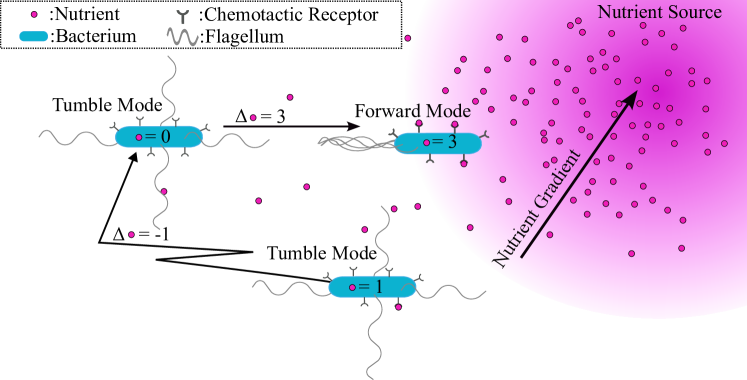
Figure 1: Schematic illustration of a CB (cyan ellipsoid) at three different time instances performing gradient sensing to locate a nutrient source (purple area) that is constantly releasing nutrients (purple dots). The CB senses its environment and switches from tumble mode to forward mode to follow a positive nutrient gradient, while switching back to tumble mode when the sensed number of nutrients decreases.

Fig. 1 illustrates the concept of bacterial chemotaxis schematically. In particular, Fig. 1 shows the same CB (cyan ellipsoid) at three different time instants seeking nutrients that are produced by a nutrient source in the top right corner. At the first time instant (center bottom), only one of the CB’s receptors is bound by a nutrient (purple dots) and it moves in tumble mode. After a random movement to the top left, the CB finds itself in a local environment with even fewer nutrients than before. Consequently, none of its receptors is bound at the second time instant, i.e., the detected nutrient gradient in the direction of movement is negative, and the CB remains in tumble mode. Finally, after (coincidentally) moving in the direction of the food source in the third time instant, the number of bound receptors exceeds the number of previously bound ones and the CB switches to run mode, aligning its future trajectory with the location of the nutrient source.

Despite its conceptual simplicity, bacterial chemotaxis presents an example of a complex adaptive system (CAS) [10]; the CB adapts to a changing environment based on the information it gathers from its surrounding, seeking to maximize its chances to survive by collecting nutrients [9]. On both a practical and a more abstract level, this observation relates the natural bacterial chemotactic system to the synthetic MC systems envisioned to operate in biological environments fulfilling complex tasks like drug delivery or early disease diagnosis. On a practical level, the ability to detect and follow a gradient of molecules in the environment that CBs possess, is desirable also for many synthetic applications. For example, autonomous drug-carrying nanodevices could be engineered to follow a gradient of biomarkers in order to deposit their therapeutic charge directly at the location of the disease. On a more abstract level, for many envisioned MC applications it is still an open question how information exchange (for example between nanodevices or between nanodevices and their environment) relates quantitatively to achieving a particular goal, e.g., cooperative early disease diagnosis or drug delivery. Since information acquisition (nutrient sensing) and goal (survival) are well-characterized in the context of bacterial chemotaxis, this provides the opportunity for developing and testing such a quantitative information theoretic framework.

As a playground for exploring these possibilities, we will introduce an existing computational bacterial chemotaxis model in the remainder of this section that we will utilize later to develop and test the semantic information theory framework proposed in this paper.

II-B Agent-based Model for Bacterial Chemotaxis

CAS, such as the bacterial chemotaxis studied in this paper, are notoriously difficult to formalize and analyze mathematically; mainly because the complex nonlinear dynamics of these systems usually emerge from (local) interactions among discrete entities with large state-spaces which are difficult or impossible to capture and analyze using analytical frameworks. However, since CASs arise in many and diverse scientific fields, ranging from economy over society to systems biology, the need for modeling their dynamics has spawned a number of innovative computational modeling tools, among which ABM is a particularly commonly used one [11]. In ABMs, computational agents interact with each other and/or the environment according to a set of pre-defined rules. The rules specify which action an agent is going to perform based on some information that it collects from other agents and/or the environment. In econometric models, the agents could, for example, model stock traders that interact with the stock market (environment) and other traders according to certain buying and selling strategies. The particular benefit of ABMs for the analysis of CASs is their exploratory power; in the example above, they can, for example, be utilized to test the impact of different trading strategies on the stock market dynamics.

In the following, we introduce an ABM for bacterial run-and-tumble-based chemotaxis which is adopted from the literature [10, 9] and simplified for our purposes. Fig. 2 illustrates the main components of the considered model. As computational domain, it features a two-dimensional lattice of size $N$-by-$N$ denoted by $\mathcal{L}=\{1,\ldots,N\}\times\{1,\ldots,N\}$ on which a CB (cyan) tries to locate nutrients (red) which are supplied by a nutrient source (pink). The state of the computational model evolves in discrete time steps $k\in\mathbb{N}_{0}$, where $\mathbb{N}_{0}$ denotes the set of non-negative integers, as a result of the actions and interactions of the components described in the following.

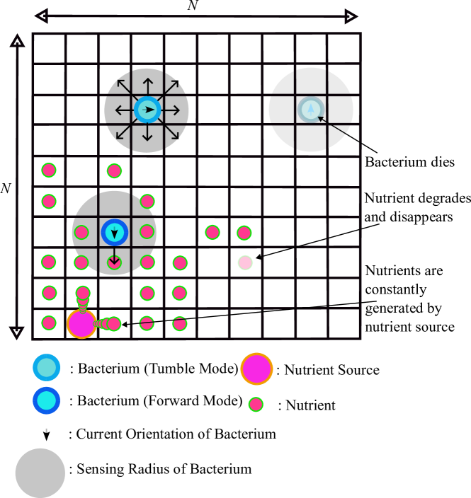
Figure 2: Considered computational bacterial chemotaxis model. Bacterium (cyan) seeks to follow nutrient source (pink) by switching between run and tumble modes according to the nutrient (red) concentrations it observes in its local environment.

II-B1 Model for Nutrient Source

The ABM features one nutrient source whose purpose is to supply the environment with nutrients. The location of the nutrient source in time step $k$ is denoted by $\mathbf{s}[k]\in\mathcal{L}$. In each time step, the nutrient source produces nutrients at rate $k_{\mathrm{NS}}$ [nutrients/time step] which are placed randomly on one of the neighboring grid cells next to $\mathbf{s}[k]$, where the distance between two grid cells $\mathbf{c}_{1}=[i_{1},j_{1}]\in\mathcal{L}$ and $\mathbf{c}_{2}=[i_{2},j_{2}]\in\mathcal{L}$ is defined as $d(\mathbf{c}_{1},\mathbf{c}_{2})=\max\{|i_{1}-i_{2}|,|j_{1}-j_{2}|\}$. See also Fig. 2 for an illustration of this process. In our model, there can be only one nutrient in a grid cell. Therefore, if the randomly selected grid cell is already occupied by another nutrient, that nutrient will be pushed away (and possibly pushes another nutrient, and so on and so forth). Only if this procedure fails, e.g., causes a deadlock, another neighboring grid cell is randomly selected. In addition to producing nutrients, the nutrient source is mobile and changes its location randomly every $m$ time steps to a new position $\mathbf{s}[k+m]$ at a distance $d_{\mathrm{max}}$, i.e., $d(\mathbf{s}[k],\mathbf{s}[k+m])\leq d_{\mathrm{max}}$. The mobility of the nutrient source resembles the variability of the food supply in natural systems and challenges the food-seeking bacterium to follow its trajectory; the higher the mobility of the nutrient source, the more challenging it is for the bacterium to adapt.

II-B2 Model for Nutrient

The nutrients produced by the nutrient source remain at their spawning positions (if not being pushed) and vanish randomly after a minimum number of time steps $K_{\mathrm{deg}}=10$. The vanishing of the nutrients from the grid resembles the degradation of nutrients in biological systems. Let $N_{Y}[k]$ denote the number of nutrients at time step $k$. Then, the positions of all nutrients at $k$ are collected in vector $\mathbf{Y}[k]=[\mathbf{Y}_{1}^{(k)},\ldots,\mathbf{Y}_{N_{Y}[k]}^{(k)}]\in\mathcal{L}^{N_{Y}[k]}$.

II-B3 Model for Bacteria

Similar to the biological CBs discussed at the beginning of this section, the computational CB (agent), scans its local environment for food and adapts its movement strategy according to the sensed nutrient concentration. Let us denote the position of the CB at time step $k$ by $\mathbf{x}[k]\in\mathcal{L}$. Then, the CB counts the number of nutrients on the neighboring grid cells, $N^{o}[k]$, as $N^{o}[k]=|\{\mathbf{Y}_{l}^{(k)}\,|\,d(\mathbf{Y}_{l}^{(k)},\mathbf{x}[k])\leq 1,1\leq l\leq N_{Y}[k]\}|$, where $|\mathcal{A}|$ denotes the cardinality of set $\mathcal{A}$. Finally, as illustrated in Fig. 2, the CB traverses $\mathcal{L}$ in one of two modes, the tumble mode or the run mode, resembling the two operating modes of biological CBs as discussed above. It switches into tumble mode in time step $k$ if $N^{o}[k]<N^{o}[k-1]$ or $N^{o}[k]=0$ and into run mode otherwise. In tumble mode, $\mathbf{x}[k+1]\in\mathcal{L}$ is selected randomly such that $d(\mathbf{x}[k+1],\mathbf{x}[k])=1$, i.e., the CB randomly moves to one of the neighboring grid cells. In run mode, $\mathbf{x}[k+1]=[\mathbf{x}[k]+(\mathbf{x}[k]-\mathbf{x}[k-1])]_{\mathcal{L}}$, where the notation $[\mathbf{x}]_{\mathcal{L}}$ indicates that vector $\mathbf{x}$ is mapped towards the nearest location inside $\mathcal{L}$; hence, in run mode, the CB continues its previous movement direction straight unless it hits a boundary from which it is reflected. If, due to a reflection at the boundary of $\mathcal{L}$, $\mathbf{x}[k]=\mathbf{x}[k-1]$, the CB resets its current direction to a new random direction, i.e., in the next time step, $\mathbf{x}[k+1]\in\mathcal{L}$ is selected randomly such that $d(\mathbf{x}[k+1],\mathbf{x}[k])\leq 1$. The CB also possesses a weight, which is initially $1$, and decreases by an amount of $0.05$ in each time step. Moreover, the weight increases by a constant amount of $0.2$ (up to a maximum value of $1$) each time $\mathbf{x}[k]$ coincides with one of the nutrient positions $\mathbf{Y}[k]$. When the weight of the CB reaches $0$, the CB dies and can no longer move.

We note that the computational CB model considered here is rather simple, but can easily be extended in future work, e.g., by considering (i) noisy intra-cellular signal propagation, (ii) memory in the CB’s decision making [12], (iii) the energy costs to acquire and store information [13], (iv) more sophisticated gradient detection methods, e.g., the spatial gradient sampling method, where the receptor position and state (bound or unbound) is utilized for aligning the CB’s movement direction with the location of the nutrient source, from [14], and/or (i) infotaxis detection methods, where the search trajectories feature ‘zigzagging’ paths [15]. In fact, the semantic information theory framework presented in the following section even allows for the comparative analysis of these and further CB models, since it relies directly only on the observed behavior of the CB and only indirectly on its specific food-seeking strategy.

III Information Theory Framework

In this section, we will briefly outline the general semantic information framework for physical non-equilibrium systems proposed in [8] and then specialize this framework to the considered computational bacterial chemotaxis model.

III-A Semantic Information in Bio-Physical Systems

To motivate the following discussion and definitions, let us consider first on an abstract level what is the meaning (or significance) of information for CBs. Ultimately, the goal of information acquisition (cf. discussion of the effectiveness level of communication in Section I) for a CB is to choose its actions in line with its own state and the state of the environment in order to maximize its survival chances. From this point of view, we conclude that from all the information that the CB gathers about its environment, only that part carries significance which helps the CB to align its actions with its own state and the state of its environment. The semantic information framework outlined in the following builds upon this observation in the sense that it measures only that information that actually carries significance in the above sense.

Rooted in the theory of dynamic physical systems, the authors in [8] propose the transfer entropy between a dynamical system $\mathcal{X}$ and its dynamical environment $\mathcal{Y}$ as a sensible measure of the degree to which $\mathcal{X}$ is able to adapt to $\mathcal{Y}$ as both change over time. In this context, $\mathcal{X}$ and $\mathcal{Y}$ are characterized at any time $k$ by their states $X_{k}\in\mathcal{A}_{\mathcal{X}}$ and $Y_{k}\in\mathcal{A}_{\mathcal{Y}}$, respectively; under the assumption that state spaces $\mathcal{A}_{\mathcal{X}}$ and $\mathcal{A}_{\mathcal{Y}}$ are discrete, the joint dynamics of $\mathcal{X}$ and $\mathcal{Y}$ are then defined by the transition probabilities $\mathrm{Pr}\left\{X_{k+1},Y_{k+1}\,|\,X_{k},Y_{k}\right\}$ and the initial distribution $\mathrm{Pr}\left\{X_{0},Y_{0}\right\}$. Then, the transfer entropy between $\mathcal{X}$ and $\mathcal{Y}$ accumulated over $k\leq k^{\prime}$ is defined as

$$\mathcal{T}[k^{\prime}]=\sum_{k=0}^{k^{\prime}-1}I(X_{k+1};Y_{k}|X_{k}),$$ (1)

where $I(X_{k+1};Y_{k}|X_{k})$ denotes the conditional mutual information between the system’s future state $X_{k+1}$ and the present state of the environment $Y_{k}$ given the present state of the system $X_{k}$. In (1), $I(X_{k+1};Y_{k}|X_{k})$ is computed using the conditional probability mass function (pmf) $p_{k}(x_{2}\,|\,x_{1},y_{1})=\mathrm{Pr}\left\{X_{k+1}=x_{2}\,|\,X_{k}=x_{1},Y_{k}=y_{1}\right\}$, where $x_{1},x_{2}\in\mathcal{A}_{\mathcal{X}}$ and $y_{1}\in\mathcal{A}_{\mathcal{Y}}$, and the marginal probabilities of $Y_{k}$, $\mathrm{Pr}\left\{Y_{k}\right\}$.

We note that $p_{k}(x_{2}\,|\,x_{1},y_{1})$ results after separating the joint system-environment dynamics as follows

$$\mathrm{Pr}\left\{X_{k+1},Y_{k+1}\,|\,X_{k},Y_{k}\right\}$$

$$\quad=\mathrm{Pr}\left\{Y_{k+1}\,|\,X_{k},X_{k+1},Y_{k}\right\}\,\mathrm{Pr}\left\{X_{k+1}\,|\,X_{k},Y_{k}\right\}.$$ (2)

Introducing the short-hand notation $q_{k}(y_{2}\,|\,x_{1},x_{2},y_{1})=\mathrm{Pr}\left\{Y_{k+1}=y_{2}\,|\,X_{k}=x_{1},X_{k+1}=x_{2},Y_{k}=y_{1}\right\}$, $y_{2}\in\mathcal{A}_{\mathcal{Y}}$, (III-A) suggests that the system dynamics can be separated as $q_{k}\,p_{k}$ into the state evolution of the environment, $q_{k}$, and the action/state evolution of the system, $p_{k}$. Here, the exact forms of $p_{k}$ and $q_{k}$ depend on (a) the specific choices of $\mathcal{X}$ and $\mathcal{Y}$ and (b) how $\mathcal{X}$ and $\mathcal{Y}$ interact, i.e., mutually influence the dynamics of each other. In particular, $p_{k}$ is defined by what information $\mathcal{X}$ gathers about $Y_{k}$ and how it selects its actions accordingly.

Now, the key idea for quantifying semantic information proposed in [8] is to consider different interventions that change the way that $\mathcal{X}$ perceives (and/or reacts to) $Y_{k}$ leading to different system dynamics $p^{\iota}_{k}(x_{2}\,|\,x_{1},y_{1})$, where $\iota\in\mathcal{I}$ denotes such an intervention from the set of all possible interventions $\mathcal{I}$. One simple example for an intervention is that $\mathcal{X}$ may not be able to distinguish among a set of different system states under the intervention, while it is able to distinguish these states under normal conditions. Then, for any intervention $\iota$, the corresponding transfer entropy is defined as

$$\mathcal{T}_{\iota}[k]=\sum_{k^{\prime}=0}^{k-1}I_{\iota}(X_{k^{\prime}+1};Y_{k^{\prime}}|X_{k^{\prime}}),$$ (3)

where the conditional mutual information $I_{\iota}(X_{k+1};Y_{k}|X_{k})$ is computed from $p^{\iota}_{k}(x_{2}\,|\,x_{1},y_{1})$ and the marginal distribution of $Y_{k}$ under the intervened system dynamics $q_{k}p^{\iota}_{k}$.

In addition to quantifying the degree of interaction between $\mathcal{X}$ and $\mathcal{Y}$ via the transfer entropy, the concept of semantic information considered in [8] necessitates a scalar-valued viability function $V[k]$ that quantifies in some sense the fitness of $\mathcal{X}$ at time instant $k$. Considering different interventions $\iota\in\mathcal{I}$, we expect that $V[k]$ can be different under some intervened system dynamics as compared to the normal system dynamics, since some interventions may reduce the ability of $\mathcal{X}$ to achieve a particular viability. Hence, we denote by $V_{\iota}[k]$ the viability of $\mathcal{X}$ at time step $k$ under intervention $\iota$.

From the above definitions finally arises the measure of observed semantic information at time $k$ as the lowest amount of transfer entropy (obtained under the set of interventions $\mathcal{I}$) at which $V_{\iota}[k]$ is not significantly reduced as compared to the original dynamics of the system. Formally, the observed semantic information at time step $k$ is defined as

$$S[k]=\min\limits_{\iota\in\mathcal{I}}\left\{\mathcal{T}_{\iota}[k]\,|\,V_{\iota}[k]\geq V[k](1-\epsilon)\right\},$$ (4)

where we have slightly generalized the definition of observed semantic information from [8] to allow for a small reduction in viability relative to $V[k]$ by $\epsilon\geq 0$ that accounts for variations of the viability that are negligible in practice, which is determined by the goal of the MC-based transmission system.

We will show next in the context of the computational CBs introduced in Section II how the above abstract definitions specialize for specific choices of $\mathcal{X}$ and $\mathcal{Y}$.

III-B Semantic Information for Chemotaxis

For the computational chemotaxis system introduced in Section II-B, we first specialize $\mathcal{X}$ as the computational CB and $\mathcal{Y}$ as the nutrients, respectively. Accordingly, we define the state of the CB at time $k$ as its position $\mathbf{x}[k]$ and the state of the environment as the positions of all nutrients $\mathbf{Y}[k]$, i.e., $\mathcal{A}_{\mathcal{X}}=\mathcal{L}$ and $\mathcal{A}_{\mathcal{Y}}=\bigcup_{l=0,\ldots,N^{2}}\mathcal{L}^{l}$, where the definition of $\mathcal{A}_{\mathcal{Y}}$ results from the fact that any number of nutrients between $0$ and $N^{2}$ can exist at the same time and the empty set $\mathcal{L}^{0}=\{\}$ corresponds to the state in which no nutrients exist.

In the computational chemotaxis model, the system dynamics $q_{k}\,p_{k}$ arise from the algorithmic specifications of the CB, the nutrient source, and the nutrients. Hence, we estimate $q_{k}\,p_{k}$ by running ensemble simulations. Let $E$ denote the total number of simulation runs and let $\mathbf{x}^{e}[k]$ and $\mathbf{Y}^{e}[k]$ denote the CB’s position and the nutrients’ positions, respectively, at time $k$ in simulation run $e\in\{1,\ldots,E\}$. Then, $q_{k}\,p_{k}$ can in principle be obtained from

$$\mathrm{Pr}\left\{X_{k+1}=x_{2},Y_{k+1}=y_{2},X_{k}=x_{1},Y_{k}=y_{1}\right\}$$

$$=\lim\limits_{E\to\infty}\frac{1}{E}\sum\limits_{e=1}^{E}\mathbbm{1}_{\{x_{1}\}}\left(\mathbf{x}^{e}[k]\right)\mathbbm{1}_{\{y_{1}\}}\left(\mathbf{Y}^{e}[k]\right)$$

$$\quad{}\times\mathbbm{1}_{\{x_{2}\}}\left(\mathbf{x}^{e}[k+1]\right)\mathbbm{1}_{\{y_{2}\}}\left(\mathbf{Y}^{e}[k+1]\right),$$ (5)

where $\mathbbm{1}_{\mathcal{A}}\left(x\right)$ denotes the indicator function, i.e., $\mathbbm{1}_{\mathcal{A}}\left(x\right)=1$ if $x\in\mathcal{A}$ and $\mathbbm{1}_{\mathcal{A}}\left(x\right)=0$ otherwise. Since in practice $E$ is finite, we further denote by $q^{E}_{k}\,p^{E}_{k}$ the system dynamics obtained by evaluating the right-hand side of (III-B), but with $E$ fixed, i.e., without taking the limit. We notice from the definition of $\mathcal{A}_{\mathcal{Y}}$ that $|\mathcal{A}_{\mathcal{Y}}|$ is so large, even for moderate $N$, that $q^{E}_{k}\,p^{E}_{k}$ would converge to $q_{k}\,p_{k}$ only for very large values of $E$, rendering the required computations infeasible. To overcome this problem, we consider the reduced state space $\mathcal{A}_{\mathcal{\tilde{Y}}}=\mathcal{L}$ and map any $\mathbf{Y}[k]\in\mathcal{A}_{\mathcal{Y}}$ onto $\mathcal{A}_{\mathcal{\tilde{Y}}}$ as follows

$$\tilde{\mathbbm{1}}_{\tilde{y}}\left(\mathbf{Y}[k]\right)=\begin{cases}1,&\textrm{ if }\mathbf{Y}_{l}[k]=\tilde{y}\textrm{ for any }1\leq l\leq N_{Y}[k],\\ 0,&\textrm{otherwise},\end{cases}$$ (6)

where $\tilde{y}\in\mathcal{A}_{\mathcal{\tilde{Y}}}$. After proper normalization, we obtain

$$\mathrm{Pr}\left\{X_{k+1}=x_{2},\tilde{Y}_{k+1}=\tilde{y}_{2},X_{k}=x_{1},\tilde{Y}_{k}=\tilde{y}_{1}\right\}$$

$$=\lim\limits_{E\to\infty}\frac{1}{E}\sum\limits_{e=1}^{E}\mathbbm{1}_{\{x_{1}\}}\left(\mathbf{x}^{e}[k]\right)\frac{1}{N_{Y}[k]}\tilde{\mathbbm{1}}_{\tilde{y}_{1}}\left(\mathbf{Y}^{e}[k]\right)$$

$$\quad{}\times\mathbbm{1}_{\{x_{2}\}}\left(\mathbf{x}^{e}[k+1]\right)\frac{1}{N_{Y}[k+1]}\tilde{\mathbbm{1}}_{\tilde{y}_{2}}\left(\mathbf{Y}^{e}[k+1]\right),$$ (7)

where $\tilde{y}_{1},\tilde{y}_{2}\in\mathcal{A}_{\mathcal{\tilde{Y}}}$. According to its definition, $\mathcal{A}_{\mathcal{\tilde{Y}}}$ is equivalent to $\mathcal{A}_{\mathcal{Y}}$ for $N_{Y}=1$ and for $N_{Y}\geq 2$ it approximates states with more than one nutrient as superpositions of single-nutrient states. We will see in the results section that the reduced state space $\mathcal{A}_{\mathcal{\tilde{Y}}}$ still provides a meaningful characterization of the considered chemotactic system. Based on (III-B), we define $\tilde{q}^{E}_{k}$, $\tilde{p}^{E}_{k}$ exactly analogous to how $q^{E}_{k}$, $p^{E}_{k}$ has been defined above.

We recall that, in each time step, the computational CB introduced in the previous section senses nutrient concentration values ranging from $0$ to $9$. Now, we seek to study within the framework of interventions, cf. Section III-A, how the gathering of information from the environment impacts the ability of the CB to adapt their behavior to the environment; as one type of interventions, we consider CBs whose sensing capability is limited to $n$, $\mathrm{CB}_{n}$, where $n\in\{0,\ldots,9\}$, i.e., $\mathrm{CB}_{n}$s can only sense up to $n$ nutrients. Then, in each time step $k$, $N^{o}_{n}[k]$ denotes the number of nutrients sensed by a $\mathrm{CB}_{n}$, where

$$N^{o}_{n}[k]=\min\{N^{o}[k],n\}.$$ (8)

Based on this definition, for each $n$, we identify $\mathrm{CB}_{n}$ with one intervention $\iota=n$. For example, $\iota=0$ corresponds to $\mathrm{CB}_{0}$, i.e., the computational CB always senses $0$ nutrients independent of how many nutrients actually exist in its environment; hence, $\mathrm{CB}_{0}$ is always in tumble mode. On the other hand $\iota=9$ corresponds to the default case in which the CB senses up to $9$ nutrients in its local environment. In addition and to verify that the framework presented in this paper reflects some intuitive notion of adaptive and non-adaptive behavior, we introduce two more interventions $\iota=\mathrm{d}$ (dead) and $\iota=\mathrm{f}$ (fixed); intervention $\iota=\mathrm{d}$ kills the CB, leaving it immobile and, hence, completely insensitive to the environment. Under intervention $\iota=\mathrm{f}$, the CB remains at a fixed location throughout the simulation, but, as long as it is alive, consumes nutrients; in that case, the CB still interacts with the environment through the consumption of nutrients, but is not able to adapt its behavior to it. Intuitively, both $\iota=\mathrm{d}$ and $\iota=\mathrm{f}$, reflect scenarios in which the CB is not able to adapt to the environment and we will confirm in Section IV that the semantic information framework reflects this intuition.

Finally, we define the viability function $V[k]$ as the survival rate of the CBs at time $k$, i.e., as the percentage of simulations for which the CB was still alive at $k$.

In the following section, we will confirm that the introduced information theoretic metrics and state definitions for the computational bacterial chemotaxis provide a useful measure of the exchange of semantic information between the CB and the environment.

IV Evaluation

In the following, we present numerical results from stochastic ensemble simulations of the computational bacterial chemotaxis framework introduced in Section II-B. Furthermore, the reported information theoretic measures in this section, i.e., mutual information and transfer entropy, are evaluated based on the estimated system dynamics $\tilde{q}^{E}_{k}\,\tilde{p}^{E}_{k}$ as introduced in Section III-B. Furthermore, the initial position of the CB is randomly drawn for each realization $e$. If not noted otherwise, $E=20000$, $N=10$, $k_{\mathrm{NS}}=2$, and $\epsilon=0.1$, are used as default parameter values, complementing the default values already provided in Section II-B.

IV-A Viability Evaluation

First, we study whether the considered interventions in Section III-B are indeed sensible choices. Fig. 3 shows the viability of the CB as a function of $k$ for all considered interventions $\iota\in\mathcal{I}$. In Fig. 3, in order to suppress the impact of initial transient dynamics (before the total number of nutrients in the environment has reached its equilibrium), the interventions are applied from $k=25$ on, i.e., the joint system-environment dynamics correspond to $q_{k}\,p_{k}$ for $k<25$ and to $q^{\iota}_{k}\,p^{\iota}_{k}$ for $k\geq 25$. We observe from Fig. 3 that indeed the CB with the best sensing capability, corresponding to $\iota=9$, exhibits the largest viability over the entire considered time frame; furthermore, the viability decreases as the sensing capability of the CB decreases. Finally, we observe from Fig. 3 that the static CB ($\iota=\mathrm{f}$) possesses the smallest viability among all considered cases (except for $\iota=\mathrm{d}$, the dead bacteria, whose viability drops to $0$ in the moment the intervention is applied). An insightful metric is the difference in viability $\Delta V=V-V_{\mathrm{f}}$ between the default case, i.e., $\iota=9$, and the "strongest" intervention $\iota=\mathrm{f}$, i.e., the intervention that results in strongest non-adaptive behavior of the CB, and is therefore highlighted with a green vertical line in Fig. 3 (and in the following figures as well).

These results confirm that the choice of interventions is indeed sensible since they do indeed impact the viability of the CB.

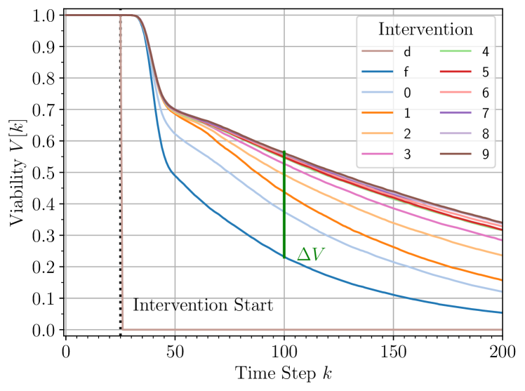
Figure 3: Viability as a function of the simulation time steps for different interventions, which start after 25 steps.

IV-B Mutual Information

In this section, we seek to confirm our definition of the CB’s and the nutrients’ states, respectively. To this end, Fig. 4 shows the mutual information $I_{\iota}(X_{k};Y_{k})$ for two different parameter sets for the movement of the nutrient source, resulting in gradual and jump movements, and different interventions $\iota$. We observe from Fig. 4 that $I_{\iota}(X_{k};Y_{k})$, i.e., the dependence between the CB’s position and the nutrients’ positions, is generally largest for $\iota=9$ for both gradually and abruptly moving nutrient sources, confirming that the CB’s sensing ability correlates with its ability to follow the moving food source. On the other hand, we observe from Fig. 4 that for $\iota=5,1$, the CB’s ability to follow the nutrient source is decreased. The wave-like patterns visible for $I_{\iota}(X_{k};Y_{k})$ for $\iota=9,5,1$ for the abruptly moving nutrient source correspond to phases of decreasing proximity between CB and nutrient source each time $\mathbf{s}[k]$ changes abruptly, followed by a phase of increasing proximity, when the CB manages to realign its position with $\mathbf{s}[k]$. Moreover, we observe from Fig. 4 that $I_{\iota}(X_{k};Y_{k})$ is approximately constant for $\iota=0,\mathrm{d},\mathrm{f}$, confirming our intuition that in these cases no significant correlation between $\mathcal{X}$ and $\mathcal{Y}$ exists.

These results confirm that for our selection of states, an information theoretic analysis of the considered system delivers sensible results.

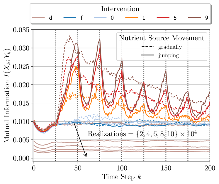
Figure 4: The mutual information as a function of the simulation time steps for different interventions, which start after 25 steps. Nutrient source movement gradually (dotted) (jumping (solid)) indicates a nutrient source moving a maximum distance of $d_{\mathrm{max}}=3$ ($d_{\mathrm{max}}=8$) every $m=5$ ($m=25$) steps. The results for intervention $\iota=\mathrm{d}$ (brown) are shown for different numbers of simulation realizations $E$.

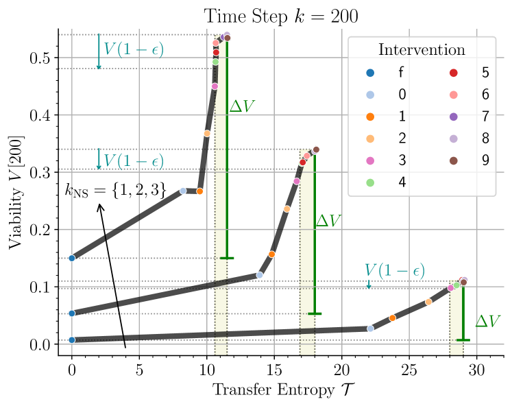
Figure 5: Transfer entropy vs. viability at time step $k=200$ for three different nutrient produce rates and different interventions. The shaded areas highlight transfer entropies of interventions resulting in (nearly) constant viability values characterized by $\epsilon$, cf. (4); the cyan arrows indicate the corresponding viability limits.

IV-C Viability vs. Transfer Entropy

Finally, Fig. 5 shows the viability and the transfer entropy $\mathcal{T}_{\iota}[k]$ at $k=200$ for different nutrient production rates $k_{\mathrm{NS}}$ under different interventions. Also, it is shown in Fig. 5 as $\Delta V$ by how much the viability differs between $\iota=\mathrm{f}$ and $\iota=9$. Several insights can be gained from Fig. 5. First, we observe from Fig. 5 that the viability is in general the higher, the more nutrients are produced. This is intuitive as more nutrients increase the chance that the CB’s position coincides with the position of a nutrient, increasing the CB’s chances to survive, cf. Section II-B3. Moreover, we observe for more nutrients a larger value of $\Delta V$, namely $\Delta V=0.39,0.287,0.004$ for $k_{\mathrm{NS}}=3,2,1$. However, considering the relative change in viability, $\Delta\tilde{V}=\Delta V/V_{9}$, for different values of $k_{\mathrm{NS}}$, we obtain $\Delta\tilde{V}=0.73,0.86,0.91$ for $k_{\mathrm{NS}}=3,2,1$, i.e., for higher selection pressure (resulting from a low number of nutrients) sensing capabilities become more essential for survival. This is also reflected in the higher transfer entropy for lower values of $k_{\mathrm{NS}}$.

Next, we observe that for all considered $k_{\mathrm{NS}}$, the transfer entropy is positively correlated with the viability; hence in all considered cases increased adaptability leads to increased viability (excluding the slight fluctuations due to the stochasticity of the numerical simulations, which are visible for $\iota=9$).

We also observe that, as the sensing capability of the CB increases from $\iota=\mathrm{f}$ to $\iota=9$, the corresponding transfer entropy increases; however, the corresponding increase in information flow, determined by $\Delta\mathcal{T}_{\iota_{1},\iota_{2}}=\mathcal{T}_{\iota_{2}}-\mathcal{T}_{\iota_{1}}$, due to changing the intervention from $\iota=\iota_{1}$ to $\iota=\iota_{2}$ (increasing the limit of detectable nutrient concentrations) is non-monotonic, which is observable for the first time in the semantic information analysis presented here. For example, we observe that for $k_{\mathrm{NS}}=2$, surprisingly $\Delta\mathcal{T}_{4,5}<\Delta\mathcal{T}_{5,6}<\Delta\mathcal{T}_{3,4}$; the semantic framework provides insights which remain elusive when using existing syntactic information metrics. Finally, we observe from Fig. 5 that, for each $k_{\mathrm{NS}}$, as the CB’s sensing capability decreases from $\iota=9$ to smaller values, the viability is first only marginally affected. For example, for $k_{\mathrm{NS}}=1$ there is only little difference in the corresponding viabilities for $\iota=9,\dots,3$, indicating that the observed semantic information $S[200]$ in that case corresponds to $\mathcal{T}_{3}[200]$.

These results show that the semantic information framework developed in this paper can deliver novel insights on the information exchange in the considered computational bacterial chemotaxis system. In particular, it is shown that the transfer entropy provides a useful measure of the ability of the CB to adapt its location to a moving nutrient source and correlates with its viability. Due to the generality of the mathematical formalism and the proposed state definitions, respectively, the proposed model can easily be extended to different computational CB models allowing for comparative analysis in unprecedented generality.

V Conclusion

In this paper, we have shown that the semantic information framework proposed originally in [8] provides indeed a useful and sensible characterization of the considered computational bacterial chemotaxis model. Specifically, our results confirm that the ability of the CB to adapt to its changing environment is accurately reflected in the proposed information theoretic measures whose evaluation relies only on observing the CB’s and the nutrients’ positions rather than on knowing their internal processes. In this regard, it provides a general, yet very practical, framework for the analysis of the considered system. Since many applications envisioned for MC share common features with the considered chemotaxis model, we envision that the considered semantic information theory framework can be utilized for the analysis and design of future MC systems.

References

- [1] W. Weaver, “Recent contributions to the mathematical theory of communication,” ETC: A Review of General Semantics, vol. 10, no. 4, pp. 261–281, 1953.
- [2] G. Shi, Y. Xiao, Y. Li, and X. Xie, “From semantic communication to semantic-aware networking: Model, architecture, and open problems,” IEEE Commun. Mag., vol. 59, no. 8, pp. 44–50, Aug. 2021.
- [3] W. Yang et al., “Semantic communications for future internet: Fundamentals, applications, and challenges,” IEEE Commun. Surv. Tutor., vol. 25, no. 1, pp. 213–250, Nov. 2022.
- [4] E. C. Strinati and S. Barbarossa, “6G networks: Beyond Shannon towards semantic and goal-oriented communications,” Comput. Netw., vol. 190, p. 107930, Mar. 2021.
- [5] I. F. Akyildiz, M. Pierobon, S. Balasubramaniam, and Y. Koucheryavy, “The Internet of Bio-Nano Things,” IEEE Commun. Mag., vol. 53, no. 3, pp. 32–40, Mar. 2015.
- [6] B. Ruzzante, L. Del Moro, M. Magarini, and P. Stano, “Synthetic cells extract semantic information from their environment,” Trans. Mol. Biol. Multi Scale Commun., vol. 9, no. 1, pp. 23–27, Feb. 2023.
- [7] T. S. Barker, P. J. Thomas, and M. Pierobon, “A metric to quantify subjective information in biological gradient sensing,” in Proc. IEEE Global Commun. Conf. (GLOBECOM). IEEE, Dec. 2023.
- [8] A. Kolchinsky and D. H. Wolpert, “Semantic information, autonomous agency and non-equilibrium statistical physics,” Interface Focus, vol. 8, no. 6, p. 20180041, Oct. 2018.
- [9] H. C. Berg, E. coli in Motion. New York, USA: Springer, 2004.
- [10] K. Nagarajan, C. Ni, and T. Lu, “Agent-based modeling of microbial communities,” ACS Synth. Biol., vol. 11, no. 11, pp. 3564–3574, Oct. 2022.
- [11] S. Abar, G. K. Theodoropoulos, P. Lemarinier, and G. M. O’Hare, “Agent based modelling and simulation tools: A review of the state-of-art software,” Computer Science Review, vol. 24, pp. 13–33, May 2017.
- [12] A. Gosztolai and M. Barahona, “Cellular memory enhances bacterial chemotactic navigation in rugged environments,” Commun. Phys., vol. 3, no. 1, p. 47, Mar. 2020.
- [13] A. J. Tjalma, V. Galstyan, J. Goedhart, L. Slim, N. B. Becker, and P. R. Ten Wolde, “Trade-offs between cost and information in cellular prediction,” Proc. Natl. Acad. Sci., vol. 120, no. 41, p. e2303078120, Oct. 2023.
- [14] J. Rode, M. Novak, and B. M. Friedrich, “Chemotactic agents combining spatial and temporal gradient-sensing boost spatial comparison if they are large, slow, and less persistent,” bioRxiv version: 2023.10.14.562229, 2023.
- [15] M. Vergassola, E. Villermaux, and B. I. Shraiman, “‘Infotaxis’ as a strategy for searching without gradients,” Nature, vol. 445, no. 7126, pp. 406–409, Jan. 2007.