Entanglement cost of discriminating quantum states under locality constraints

Abstract

The unique features of entanglement and non-locality in quantum systems, where there are pairs of bipartite states perfectly distinguishable by general entangled measurements yet indistinguishable by local operations and classical communication, hold significant importance in quantum entanglement theory, distributed quantum information processing, and quantum data hiding. This paper delves into the entanglement cost for discriminating two bipartite quantum states, employing positive operator-valued measures (POVMs) with positive partial transpose (PPT) to achieve optimal success probability through general entangled measurements. First, we introduce an efficiently computable quantity called the spectral PPT-distance of a POVM to quantify the localness of a general measurement. We show that it can be a lower bound for the entanglement cost of optimal discrimination by PPT POVMs. Second, we establish an upper bound on the entanglement cost of optimal discrimination by PPT POVMs for any pair of states. Leveraging this result, we show that a pure state can be optimally discriminated against any other state with the assistance of a single Bell state. This study advances our understanding of the pivotal role played by entanglement in quantum state discrimination, serving as a crucial element in unlocking quantum data hiding against locally constrained measurements.

1 Introduction

In the realm of quantum information, nonlocality manifests when local measurements on a multipartite quantum system may not be able to reveal in which state the system is prepared, even among mutually orthogonal product states [1]. It has consistently been a crucial research direction to understand the power and limits of quantum operations that can be implemented by local operations and classical communication (LOCC), e.g., in quantum state discrimination [2, 3, 4, 5, 6, 7, 8, 1, 9, 10].

In quantum state discrimination tasks, one usually performs a binary-valued positive-operator valued measure (POVM) on the received state and then decides which state it is according to the measurement outcome. Quantum state discrimination has led to fruitful applications in quantum cryptography [11, 12, 13], quantum dimension witness [14, 15] and quantum data hiding [16, 17, 18]. To understand the underlying mechanism of quantum state discrimination, various operations that encompass LOCC are further considered due to its complex structure, including POVMs that are separable (SEP) [19, 20], and POVMs with positive partial transpose (PPT) [21, 22, 23]. There is a strict inclusion among them as [1],

$$\text{LOCC}\subseteq\textrm{SEP}\subseteq\textrm{PPT}\subseteq\textrm{ALL}.$$ (1)

Notably, PPT POVMs enjoy a much simpler mathematical structure than LOCC and SEP as the former can be completely characterized by semidefinite programming (SDP) [24]. In particular, the distinguishability of quantum states under a restricted family of measurements is closely related to quantum data hiding [25, 26], which is originally based on the existence of pairs of bipartite states that are perfectly distinguishable with general entangled measurements yet indistinguishable by LOCC. In the context of bipartite state discrimination, the utility of a shared entangled state is paramount as it can significantly improve limited local distinguishability, potentially matching the efficacy of general entangled measurements. Notably, a maximally entangled state is often a universal resource for such enhancements [27, 3]. This leads to a compelling and crucial question:

How much entanglement at minimum do we need to unlock this quantum data hiding?

Due to the complex structure of LOCC and entanglement, our understanding of the role of entanglement in quantum state discrimination is still limited. Currently, the entanglement cost is only known for a small number of ensembles of quantum states, with a focus on the set that contains at least one of the four Bell states. Specifically, it has been shown that Bell basis [28] and a set of three Bell states [19] can be distinguished with the assistance of 1 ebit. For quantum states with higher dimensions, Ref. [21] shows that 1 ebit suffices for discriminating a $d\otimes d$ pure state and its orthogonal complement perfectly by PPT POVMs. For other special cases, Ref. [29] demonstrates that 1 ebit is required for the optimal discrimination for a noisy Bell state ensemble by LOCC.

In this paper, we study the entanglement cost of optimally discriminating two arbitrary quantum states by PPT POVMs, which is also the lower bound for the scenario of employing LOCC. Firstly, we introduce the spectral PPT-distance of a POVM which can be efficiently computed via SDP and characterizes the PPT-ness of a general POVM. Secondly, we formally define the entanglement cost of optimal discriminating a set of states via measurements under locality constraints. We show that the spectral PPT-distance of a POVM can be utilized to derive a lower bound on the entanglement cost of optimal discrimination by PPT POVMs. Thirdly, we provide an upper bound on the entanglement cost of optimal discrimination by PPT POVMs which is directly determined by the spectrum properties of the given states. Leveraging this upper bound, we show that a pure state can be optimally discriminated against any other state with the assistance of 1 ebit.

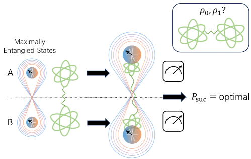
Fig 1: Illustration of the entanglement-assisted quantum state discrimination task. Alice and Bob (represented as $A$ and $B$) aim to discriminate bipartite quantum states $\rho_{0}$ and $\rho_{1}$. Commencing with an initial allocation of entanglement resources, the optimal discrimination achievable through a general entangled measurement is demonstrated to be attainable by employing measurements under locality constraints, showcasing the pivotal role of entanglement consumption in the discrimination process.

2 Preliminaries

Notations.

We use $A$ and $B$ to denote finite-dimensional Hilbert spaces ${\cal H}_{A}$ and ${\cal H}_{B}$ associated with the systems of Alice and Bob, respectively. The dimensions of ${\cal H}_{A}$ and ${\cal H}_{B}$ are denoted as $d_{A}$ and $d_{B}$. A quantum state on system $A$ is a positive semidefinite operator $\rho_{A}$ with trace one. The support of $\rho_{A}$, denoted as ${\operatorname{supp}}(\rho_{A})$, is defined as the space spanned by the eigenvectors of $\rho_{A}$ with positive eigenvalues. Let $\{|j\rangle\}_{j=0,\cdots,d-1}$ be a standard computational basis, then a standard maximally entangled state of Schmidt rank $d$ is $\Phi_{d}^{+}=1/d\sum_{i,j=0}^{d-1}|ii\rangle\!\langle jj|$. A bipartite quantum state $\rho_{AB}$ is said to be Positive-Partial-Transpose (PPT) if $\rho_{AB}^{T_{B}}\geq 0$ where $T_{B}$ denotes taking partial transpose on the subsystem $B$.

Quantum State Discrimination.

Quantum measurements are described by positive-operator-valued-measure (POVM). A POVM with $n$ elements is denoted as $\bm{E}=\{E_{j}\}_{j=0}^{n-1}$ where $E_{j}\geq 0$ and $\sum_{j}E_{j}=I$. Suppose $\Omega=\{(p_{j},\rho_{j})\}_{j=0}^{n-1}$ is an ensemble of $n$ quantum states $\rho_{0}\dots\rho_{n-1}$ given with associated probability $p_{0}\dots p_{n-1}$. In the task of quantum state discrimination, we usually apply a POVM on a given unknown state $\rho_{j}$ with prior probability $p_{j}$ and decide which state it is according to the measurement outcomes. In the context of minimum-error state discrimination (MSD), the goal is to maximize the average success probability, given by

$$P_{{\text{suc}}}(\Omega)=\max_{\{E_{j}\}}\sum_{j=0}^{n-1}p_{j}\operatorname{Tr}(\rho_{j}E_{j}).$$ (2)

Notably, the celebrated result in Ref. [30] shows that optimal discrimination success probability of discriminating two quantum states $\{\rho_{0},\rho_{1}\}$ with prior probability $p_{0}$ and $p_{1}$ is given by $\frac{1}{2}(1+\|p_{0}\rho_{0}-p_{1}\rho_{1}\|_{1})$, where $\|\cdot\|_{1}$ denotes the trace norm. The corresponding POVM is called the Helstrom measurements. It can be expressed by $M_{+}$ and $M_{-}$, where $M_{+}$ is the projection on the positive eigenspace of $p_{0}\rho_{0}-p_{1}\rho_{1}$ and $M_{-}=I-M_{+}$.

We denote ${\cal E}({\cal H}_{A})$ as the set of all positive semidefinite Hermitian matrices on ${\cal H}_{A}$ that satisfy $0\leq E\leq I,\,\forall E\in{\cal E}({\cal H}_{A})$. It is easy to see that ${\cal E}({\cal H}_{A})$ is a convex set and we will use the notation ${\cal E}$ as a shorthand for ${\cal E}({\cal H}_{A})$ when there is no ambiguity for the Hilbert space. Considering POVMs under locality constraints acting on a bipartite system $AB$, we denote ${\cal E}_{{\text{\rm LOCC}}}$ as the set of all elements of LOCC POVMs [31] which includes strategies based on measurement outcomes performed locally on each subsystem. We denote

$${\cal E}_{{\text{\rm SEP}}}({\cal H}_{A}\otimes{\cal H}_{B})\mathrel{\mathop{\mathchar 58\relax}}=\left\{E_{A}^{(k)}\otimes E_{B}^{(k)}\mathrel{\mathop{\mathchar 58\relax}}E_{A}^{(k)}\geq 0,E_{B}^{(k)}\geq 0,\sum_{k}E_{A}^{(k)}\otimes E_{B}^{(k)}=I\right\}$$ (3)

as the set of all elements for SEP POVMs [32] and

$${\cal E}_{{\text{\rm PPT}}}({\cal H}_{A}\otimes{\cal H}_{B})\mathrel{\mathop{\mathchar 58\relax}}=\left\{E_{AB}\mathrel{\mathop{\mathchar 58\relax}}0\leq E_{AB}\leq I_{AB},\,0\leq E_{AB}^{T_{B}}\leq I_{AB}\right\}$$ (4)

as the set of all elements for PPT POVMs [32].

3 Spectral PPT-distance of a POVM

To investigate the capability of measurements under locality constraints, we first focus on the characterization of the localness of a POVM. In light of the favorable mathematical characterization of PPT POVMs, we introduce the generalized PPT-distance of a POVM as follows.

Definition 1 (Generalized PPT-distance)

Given a POVM $\bm{M}=\{M_{j}\}_{j=0}^{n-1}$ acting on a bipartite system ${\cal H}_{A}\otimes{\cal H}_{B}$, its generalized PPT-distance is defined as

$$\mathscr{D}(\bm{M})=\min\bigg{\{}r\,\bigg{|}\,\Delta(M_{j}^{T_{B}},E_{j}^{T_{B}})\leq r,\,\sum_{j=0}^{n-1}E_{j}=I,E_{j}\in{\cal E}_{{\text{\rm PPT}}},\,\forall j\bigg{\}},$$ (5)

where $\Delta(\cdot,\cdot)$ is a metric that satisfies positive-definiteness, symmetry, and triangle inequality. The minimization ranges over all possible $\{E_{j}\}_{j}$.

Particularly, an essential metric is the distance induced by the Schatten $p$-norms, i.e.,

$$\left\|X\right\|_{p}=\left(\operatorname{Tr}\left[(X^{\dagger}X)^{\frac{p}{2}}\right]\right)^{\frac{1}{p}},\,p\in[1,\infty).$$ (6)

This family includes the three most commonly used distances in quantum information theory, i.e., the trace distance, the Frobenius distance, and the spectral distance. The Schatten-$p$ PPT-distance is denoted as $\mathscr{D}_{p}(\bm{M})$ for $\Delta(M_{j}^{T_{B}},E_{j}^{T_{B}})\mathrel{\mathop{\mathchar 58\relax}}=\|M_{j}^{T_{B}}-E_{j}^{T_{B}}\|_{p}$. Its geometric interpretation is depicted in Fig. 2. For $p=\infty$ where $\|\cdot\|_{\infty}$ corresponds to a fundamentally important norm of the spectral norm, we have the spectral PPT-distance of a POVM as follows.

Definition 2 (Spectral PPT-distance)

Given a POVM $\bm{M}=\{M_{j}\}_{j=0}^{n-1}$ acting on a bipartite system ${\cal H}_{A}\otimes{\cal H}_{B}$, its spectral PPT-distance is defined as

$$\mathscr{D}_{\infty}(\bm{M})=\min\bigg{\{}\,r\,\bigg{|}\,\left\|M_{j}^{T_{B}}-E_{j}^{T_{B}}\right\|_{\infty}\leq r,\,\sum_{j=0}^{n-1}E_{j}=I,E_{j}\in{\cal E}_{{\text{\rm PPT}}},\,\forall j\bigg{\}},$$ (7)

where the minimization ranges over all possible $\{E_{j}\}_{j}$.

The spectral PPT-distance of a POVM bears nice properties. Firstly, it is efficiently computable via SDP and quantifies the proximity of a given POVM to the set of PPT POVMs. Specifically, $\mathscr{D}_{\infty}(\bm{M})$ is faithful, i.e., $\mathscr{D}_{\infty}(\bm{M})\geq 0$ and $\mathscr{D}_{\infty}(\bm{M})=0$ if and only if $\bm{M}$ is a PPT POVM. Secondly, it is invariant under local unitaries which is directly obtained by the local unitary invariance of the spectral norm and PPT-ness of $E_{j}$. Thirdly, for two POVMs $\bm{M}_{0}=\{M_{0,j}\}_{j=0}^{n-1}$ and $\bm{M}_{1}=\{M_{1,j}\}_{j=0}^{n-1}$, we denote a convex combination of them as $\widehat{\bm{M}}=\alpha\bm{M}_{0}+(1-\alpha)\bm{M}_{1}\mathrel{\mathop{\mathchar 58\relax}}=\{\widehat{M_{j}}\}_{j=0}^{n-1}$ where $\widehat{M_{j}}=\alpha M_{0,j}+(1-\alpha)M_{1,j}$; denote the tensor product of them as $\widetilde{\bm{M}}=\bm{M}_{0}\otimes\bm{M}_{1}\mathrel{\mathop{\mathchar 58\relax}}=\{\widetilde{M}_{jk}\}_{j,k=0}^{n-1}$ where $\widetilde{M}_{jk}=M_{0,j}\otimes M_{1,k}$. We show that $\mathscr{D}_{\infty}(\bm{M})$ is convex w.r.t. the convex combination and linearly subadditive w.r.t. the tensor product of POVMs.

Proposition 1 (Convexity)

For POVMs $\bm{M}_{0},\bm{M}_{1}$ acting on a bipartite system ${\cal H}_{A}\otimes{\cal H}_{B}$ and $0\leq\alpha\leq 1$,

$$\mathscr{D}_{\infty}(\alpha\bm{M}_{0}+(1-\alpha)\bm{M}_{1})\leq\alpha\cdot\mathscr{D}_{\infty}(\bm{M}_{0})+(1-\alpha)\cdot\mathscr{D}_{\infty}(\bm{M}_{1}).$$ (8)

Proposition 2 (Linearly subadditivity)

For POVMs $\bm{M}_{0}=\{M_{0,j}\}_{j},\;\bm{M}_{1}=\{M_{1,k}\}_{k}$ acting on a bipartite system ${\cal H}_{A}\otimes{\cal H}_{B}$,

$$\mathscr{D}_{\infty}(\bm{M}_{0}\otimes\bm{M}_{1})\leq\xi\cdot\mathscr{D}_{\infty}(\bm{M}_{0})+\zeta\cdot\mathscr{D}_{\infty}(\bm{M}_{1}),$$ (9)

where $\xi=\max_{k}(1+\|M_{1,k}^{T_{B}}\|_{\infty})/2$ and $\zeta=\max_{j}(1+\|M_{0,j}^{T_{B}}\|_{\infty})/2$.

4 Entanglement cost of PPT discrimination

Now, we study the amount of entanglement required to discriminate a set of quantum states by PPT POVMs optimally. Herein, optimality refers to achieving the maximal average success probability without any restrictions on POVMs. We note the spectral PPT-distance of a POVM provides insights into the minimum amount of entanglement required to promote a PPT POVM to the given POVM. We will demonstrate this aspect through its application in quantum state discrimination tasks in the following.

Recall the optimal average success probability of discriminating two quantum states is given by Eq. (2) when there are no restrictions on the POVM one is allowed to perform. However, an inherent challenge that arises in practice is the spatial distribution of quantum facilities, leading to the constraint that each laboratory can execute local quantum operations with mutual classical communication available. This motivates us to consider POVMs under locality constraints, including LOCC POVMs, SEP POVMs, and PPT POVMs as illustrated in Eq. (1). Despite extensive research characterizing the minimum amount of entanglement required to discriminate quantum states by POVMs under locality constraints [21, 19, 33, 34, 29], a quantitative analysis is still lacking. To address this problem, we first introduce the entanglement-assisted average success probability where two parties are allowed to share entanglement to assist their QSD tasks.

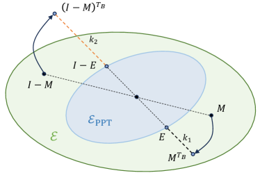
Fig 2: The spectral PPT-distance of a given binary-valued POVM $\bm{M}=\{M,I-M\}$. It is defined as the minimum spectral distance from the partial transpose of $M,I-M$ to the set of PPT POVMs. That is, $\mathscr{D}_{\infty}(\bm{M})=\min\max\{k_{1},k_{2}\}$ where the minimization ranges over all possible choices of $E,I-E\in{\cal E}_{{\text{\rm PPT}}}$. Each POVM is associated with a pair of points in the set, connected by a dashed line that intersects the origin point $I/2$.

Definition 3 (Entanglement-assisted average success probability)

Given a quantum state ensemble $\Omega=\{(p_{j},\rho_{j})\}_{j=0}^{n-1}$, where $p_{j}\geq 0$ and $\sum_{j}p_{j}=1$, and a positive integer $k\geq 2$, the entanglement-assisted average success probability of discriminating $\Omega$ via operation class $\Pi$ is defined as

$$P_{{\text{suc}},e}^{\Pi}(\Omega;k)=\max_{\{E_{j}\}\in\Pi}\sum_{j=0}^{n-1}p_{j}\operatorname{Tr}[E_{j}(\rho_{j}\otimes\Phi_{k}^{+})],$$ (10)

where $\{E_{j}\}_{j=0}^{n-1}$ is a POVM, $\Pi\in\{{\text{\rm LOCC}},{\text{\rm SEP}},{\text{\rm PPT}}\}$.

We also denote $P_{{\text{suc}}}^{\Pi}(\Omega)$ as the optimal average success probability when using POVMs in $\Pi$. Then it is natural to formally define the entanglement cost of optimal $\Pi$-discrimination by considering how much entanglement it needs to render this entanglement-assisted average success probability identical to the original optimal success probability with no restrictions on POVMs.

Definition 4 (Entanglement cost of optimal $\Pi$-discrimination)

Given a quantum state ensemble $\Omega=\{(p_{j},\rho_{j})\}_{j=0}^{n-1}$, where $p_{j}\geq 0$ and $\sum_{j}p_{j}=1$, the entanglement cost of optimal $\Pi$-discrimination is defined as

$$E^{\Pi}_{C}(\Omega)=\min\left\{\log k\mathrel{\mathop{\mathchar 58\relax}}P_{{\text{suc}},e}^{\Pi}(\Omega;k)=P_{{\text{suc}}}(\Omega),k\geq 2\right\}.$$ (11)

If $P_{{\text{suc}}}^{\Pi}(\Omega)=P_{{\text{suc}}}(\Omega)$, then $E^{\Pi}_{C}(\Omega)$ is set to be zero.

Throughout the paper, we take the logarithm to be base two unless stated otherwise. In particular, consider the scenario of discriminating a pair of quantum states $\rho_{0}$ and $\rho_{1}$ given with the same prior probability as the results for asymmetric probabilities can be easily generalized. We write the entanglement-assisted average success probability of discriminating $\rho_{0}$ and $\rho_{1}$ by PPT POVMs as $P_{{\text{suc}},e}^{{\text{\rm PPT}}}(\rho_{0},\rho_{1};k)$ and establish its SDP form in the following Proposition 3. The derivation of its dual form can be found in Appendix A.

Proof.

By definition, the entanglement-assisted average success probability by PPT POVMs can be computed via the following SDP,

$$P_{{\text{suc}},e}^{{\text{\rm PPT}}}(\rho_{0},\rho_{1};k)=\max \;\frac{1}{2}+\frac{1}{2}\operatorname{Tr}\Big{[}E[(\rho_{0}-\rho_{1})\otimes\Phi_{k}^{+}]\Big{]}$$

$${\rm s.t.} \;\;0\leq E^{T_{BB^{\prime}}}\leq I,$$ (13)

$$\;\;0\leq E\leq I,$$

where $\Phi^{+}_{k}$ is the maximally entangled state on ${\cal H}_{A^{\prime}}\otimes{\cal H}_{B^{\prime}}$ with $d_{A^{\prime}}=d_{B^{\prime}}=k$. To further simplify the optimization problem, we notice that we can write

$$\operatorname{Tr}[E((\rho_{0}-\rho_{1})\otimes\Phi_{k}^{+})]=\operatorname{Tr}[(\rho_{0}-\rho_{1})\operatorname{Tr}_{A^{\prime}B^{\prime}}((I_{AB}\otimes\Phi_{k}^{+})E)].$$ (14)

Suppose $\widetilde{E}$ is an optimal solution. Since $\Phi_{k}^{+}$ is invariant under any local unitary $U_{A^{\prime}}\otimes U^{*}_{B^{\prime}}$, i.e., $(U_{A^{\prime}}\otimes U^{*}_{B^{\prime}})\Phi_{k}^{+}(U_{A^{\prime}}\otimes U^{*}_{B^{\prime}})^{\dagger}=\Phi_{k}^{+}$, $(U_{A^{\prime}}\otimes U^{*}_{B^{\prime}})E(U_{A^{\prime}}\otimes U^{*}_{B^{\prime}})^{\dagger}$ is also an optimal solution. Since any convex combination of optimal solutions remains optimal, we have that

$$\int dU(U_{A^{\prime}}\otimes U^{*}_{B^{\prime}})E(U_{A^{\prime}}\otimes U^{*}_{B^{\prime}})^{\dagger}$$ (15)

is optimal, where $dU$ is the Haar measure. Then according to Schur’s lemma, we can restrict the optimal $\widetilde{E}$ as

$$\widetilde{E}=W_{AB}\otimes\Phi_{k}^{+}+Q_{AB}\otimes(I-\Phi_{k}^{+}),$$ (16)

with certain linear operators $W_{AB}$ and $Q_{AB}$. It follows that

$$\operatorname{Tr}_{A^{\prime}B^{\prime}}[(I_{AB}\otimes\Phi_{k}^{+})\widetilde{E}]=\operatorname{Tr}_{A^{\prime}B^{\prime}}[(I_{AB}\otimes\Phi_{k}^{+})(W_{AB}\otimes\Phi_{k}^{+}+Q_{AB}\otimes(I-\Phi_{k}^{+}))]=W_{AB},$$ (17)

which can simplify the objective function as

$$\operatorname{Tr}\left[(\rho_{0}-\rho_{1})\otimes\Phi_{k}^{+}\right]=\operatorname{Tr}\left[(\rho_{0}-\rho_{1})W_{AB}\right].$$ (18)

By spectral decomposition, we have $(\Phi_{k}^{+})^{T_{B}}=\left(P_{+}-P_{-}\right)/k$, where $P_{+}$ and $P_{-}$ are the symmetric and anti-symmetric projections respectively. Then it follows that

$$\widetilde{E}^{T_{BB^{\prime}}} =W_{AB}^{T_{B}}\otimes(\Phi_{k}^{+})^{T_{B^{\prime}}}+Q_{AB}^{T_{B}}\otimes\left(I-\Phi_{k}^{+}\right)^{T_{B^{\prime}}}$$ (19)

$$=W_{AB}^{T_{B}}\otimes\frac{P_{+}-P_{-}}{k}+Q_{AB}^{T_{B}}\otimes\frac{(k-1)P_{+}+(k+1)P_{-}}{k}$$

$$=\left[W_{AB}^{T_{B}}+(k-1)Q_{AB}^{T_{B}}\right]\otimes\frac{P_{+}}{k}+\left[-W_{AB}^{T_{B}}+(k+1)Q_{AB}^{T_{B}}\right]\otimes\frac{P_{-}}{k}.$$

Since $P_{+}$ and $P_{-}$ are positive and orthogonal to each other, we have $0\leq\widetilde{E}^{T_{BB^{\prime}}}\leq I$ if and only if

$$0\leq W_{AB}^{T_{B}}+(k-1)Q_{AB}^{T_{B}}\leq kI_{AB},$$ (20)

$$0\leq-W_{AB}^{T_{B}}+(k+1)Q_{AB}^{T_{B}}\leq kI_{AB}.$$

Similarly, we have $0\leq\widetilde{E}\leq I$ if and only if

$$0\leq W_{AB}\leq I_{AB},\;0\leq Q_{AB}\leq I_{AB}$$ (21)

Combining equations (20) and (21), the entanglement cost of optimal PPT-discrimination can be simplified and calculated by the optimization problem.     $\sqcap$$\sqcup$

Based on Proposition 3, the entanglement cost of optimal PPT-discrimination of $\rho_{0},\rho_{1}$ can be formulated as the following optimization problem.

$$E^{{\text{\rm PPT}}}_{C}(\rho_{0},\rho_{1})=\log \min\;\lceil k\rceil$$ (22)

$$\text{ s.t. }\left\{\begin{aligned} &\;W_{j},Q_{j}\in{\cal E},\,j=0,1,\\ &\;W_{0}+W_{1}=Q_{0}+Q_{1}=I,\\ &\;\operatorname{Tr}\left[(\rho_{0}-\rho_{1})W_{0}\right]=\frac{1}{2}\|\rho_{0}-\rho_{1}\|_{1},\\ &-kQ_{j}^{T_{B}}\leq W_{j}^{T_{B}}-Q_{j}^{T_{B}}\leq kQ_{j}^{T_{B}}.\\ \end{aligned}\right.$$

where $k\geq 2$. If $\rho_{0},\rho_{1}$ can be perfectly discriminated by PPT POVMs, $E^{{\text{\rm PPT}}}_{C}(\rho_{0},\rho_{1})$ is set to be zero. Notably, the optimization problem in Eq. (22) is not a valid SDP. However, the spectral PPT-distance of a POVM can be a lower bound for the entanglement cost of optimal PPT-discrimination and LOCC-discrimination.

Proof.

By the definition of the spectral PPT-distance of a given POVM, we can write the optimization problem in Eq. (23) as

$$\log\,\min \lceil k\rceil$$ (24)

s.t. $$W_{j},Q_{j}\in{\cal E},\,j=0,1,$$

$$W_{0}+W_{1}=Q_{0}+Q_{1}=I,$$

$$\operatorname{Tr}\left[(\rho_{0}-\rho_{1})W_{0}\right]=\frac{1}{2}\|\rho_{0}-\rho_{1}\|_{1},$$

$$\,Q_{j}\in{\cal E}_{{\text{\rm PPT}}},-kI\leq W_{j}^{T_{B}}-Q_{j}^{T_{B}}\leq kI,\forall j.$$

Notice that each feasible solution for the above optimization problem is a feasible solution to the problem in Eq. (22) where we use the fact that $-kQ_{j}^{T_{B}}\leq W_{j}^{T_{B}}-Q_{j}^{T_{B}}\leq kQ_{j}^{T_{B}},\forall j$ implying $Q_{j}\in{\cal E}_{{\text{\rm PPT}}},\forall j$. Hence we obtain the inequality in Eq. (23).     $\sqcap$$\sqcup$

Proposition 4 reveals that an optimal general entangled POVM having the minimum spectral PPT-distance can be used to derive a lower bound on the entanglement cost of optimal PPT-discrimination. In the following, we further present an upper bound on the entanglement cost of optimal PPT-discrimination for two arbitrary quantum states.

We leave the proof in Appendix B. Notably, Theorem 5 provides an easy-to-compute upper bound for the entanglement cost of optimal PPT-discrimination of a given pair of quantum states $\{\rho_{0},\rho_{1}\}$ with equal prior probability, which only relies on the spectrum properties of the given states. Consequently, this upper bound can be directly determined by the ranks of $\rho_{0}$ and $\rho_{1}$ as the following corollary.

Corollary 6

For two bipartite quantum states $\rho_{0},\rho_{1}$ with $\operatorname{Rank}\rho_{0}=r_{0}\leq r_{1}=\operatorname{Rank}\rho_{1}$,

$$E_{C}^{{\text{\rm PPT}}}(\rho_{0},\rho_{1})\leq\log\eta,$$ (26)

where $\eta=\max\{2r_{0}-1,r_{0}+1\}$.

Remark 1 We remark there is an intriguing connection between the entanglement cost of optimal PPT-discrimination and quantum data hiding [35]. Quantum data hiding demonstrates the existence of bipartite state pairs optimally distinguishable by general entangled POVMs but not by locally constrained sets of measurements, e.g., LOCC, SEP, and PPT POVMs. This underscores a discernible gap in the efficacy of message decoding when encoded in pairs of states and the receiver is constrained to limited classes of POVMs. These can be understood by the data-hiding procedures depending on the given physical setting, e.g., two quantum devices for decoding information cannot generate reliable entanglement. For quantum data hiding associated with PPT POVMs, the data hiding ratio [26] against PPT POVMs is given by

$$R({\text{\rm PPT}})=\max_{\{\rho_{0},\rho_{1},p\}}\frac{\|p\rho_{0}-(1-p)\rho_{1}\|_{\text{ALL}}}{\|p\rho_{0}-(1-p)\rho_{1}\|_{{\text{\rm PPT}}}},$$ (27)

which quantifies the disparity between the capabilities of global POVMs and PPT POVMs in QSD. We showcase that the strategic use of maximally entangled states in QSD tasks serves as a key to unveiling these distinctions in message decoding capabilities between general entangled measurements and PPT POVMs. In particular, Ref. [18] establishes a lower bound for $R({\text{\rm PPT}})$ with $R({\text{\rm PPT}})\geq(d+1)/2$ considering a bipartite system ${\cal H}_{d}\otimes{\cal H}_{d}$. Subsequently, Corollary 6 shows that, in a worst case, $2+\log d$ ebits suffice to fully unlock the encoded information.

In the following, we shall show that when one of the states in $\{\rho_{0},\rho_{1}\}$ is pure, a single Bell state suffices to fully unlock the quantum data hiding against PPT POVMs, i.e., the optimal PPT-discrimination can always be achieved with the assistance of 1 ebit.

Proposition 7

For bipartite quantum states $\rho_{0}$ and $\rho_{1}$, if one of them is a pure state, then

$$E_{C}^{{\text{\rm PPT}}}(\rho_{0},\rho_{1})\leq 1.$$ (28)

Proof.

Without loss of generality, suppose $\rho_{0}$ is a pure state. According to Lemma S2, we have that the projection $M_{+}$ onto the positive eigenspace of $\rho_{0}-\rho_{1}$ satisfies $\operatorname{Rank}M_{+}=1$. By Corollary 6, we have the optimal discrimination can be achieved with $E_{C}^{{\text{\rm PPT}}}(\rho_{0},\rho_{1})=1$.     $\sqcap$$\sqcup$

Proposition 7 establishes that any $d$-dimensional pure state can be optimally discriminated against any other state with the assistance of one Bell state. This result recovers and extends the previous result that one Bell state is enough for discriminating any $d$-dimensional pure state and its orthogonal complement [21]. Intriguingly, we observe that a single Bell state is not always enough for optimally discriminating an arbitrary pair of quantum states by PPT POVMs or LOCC.

Proposition 8

There exists a pair of bipartite states $\{\rho,\sigma\}$ for which the optimal discrimination concerning general entangled POVMs is not achievable by LOCC with the assistance of a single Bell state.

This phenomenon is illustrated through a numerical example provided in Appendix D, wherein we showcase a pair of two-qutrit quantum states that, even with the aid of a single Bell state, cannot be optimally discriminated by PPT POVMs. A detailed proof is deferred to Appendix D. Moreover, we note that when two states are orthogonal mixed states, the optimal PPT-discrimination can be achieved with the assistance of $\log(d-1)$ ebits.

Proposition 9

For any two orthogonal $d$-dimensional mixed bipartite quantum states $\rho_{0}$ and $\rho_{1}$,

$$E_{C}^{{\text{\rm PPT}}}(\rho_{0},\rho_{1})\leq\log(d-1).$$ (29)

Proof.

Denote the rank of $\rho_{0}$, $\rho_{1}$ as $\operatorname{Rank}\rho_{0}=r_{0}$ and $\operatorname{Rank}\rho_{1}=r_{1}$, respectively. Since $\rho_{0}$ and $\rho_{1}$ are mutually orthogonal, we have $r_{0}+r_{1}\leq d$. Suppose that $r_{0}\leq r_{1}$, we have that $\max r_{0}=d/2$. According to Corollary 6, we can conclude that $E_{C}^{{\text{\rm PPT}}}(\rho_{0},\rho_{1})\leq\log(d-1)$.     $\sqcap$$\sqcup$

5 Discussion

In this work, we delve into quantifying the entanglement cost for optimally discriminating bipartite quantum states under locality constraints. We introduce the spectral PPT-distance of a POVM and utilize it to derive a lower bound on the entanglement cost of optimal discrimination by PPT POVMs. Furthermore, we provide an upper bound based on the spectrum properties of the given states and apply it to extend the previous results on discriminating a pure state against another one. Notably, our results underscore that $2+\log d$ ebits are enough to unlock the quantum data hiding against PPT POVMs in a bipartite system ${\cal H}_{d}\otimes{\cal H}_{d}$. If the data encoding involves a pure state, then a single Bell state is sufficient.

An intriguing direction for future research lies in further analysis of quantum resource manipulation for state discrimination, e.g., within the framework of resource theories of coherence and magic states. Specifically, the study of constrained families of POVMs, such as incoherent POVMs [36] and those with positive Wigner functions [37], presents a promising avenue. Additionally, the exploration of resource manipulation in quantum state discrimination, with respect to thermodynamics [38, 39] and imaginarity [40], could pave the way for novel insights into the interplay between quantum resources and measurement processes.

Appendix A Dual of Entanglement-Assisted Average Success Probability

For simplicity, we ignore the system symbols, i.e. $W_{AB}=W$. By introducing the Lagrange multiplier $A$, $C$, $D$, $F$,$G$,$H$, the Lagrange function of the primal problem is

$$L(A,B,C,D,F,G)$$

$$=\frac{1}{2}+\frac{1}{2}\operatorname{Tr}[(\rho_{0}-\rho_{1})W]-\langle A,W-I\rangle-\langle B,Q-I\rangle$$

$$\quad-\langle C,(1-k)Q^{T_{B}}-W^{T_{B}}\rangle-\langle D,W^{T_{B}}-(1+k)Q^{T_{B}}\rangle$$

$$\quad-\langle F,(1+k)Q^{T_{B}}-kI-W^{T_{B}}\rangle-\langle G,W^{T_{B}}-kI+(k-1)Q^{T_{B}}\rangle$$

$$=\frac{1}{2}+\frac{1}{2}\operatorname{Tr}[(\rho_{0}-\rho_{1})W]-\langle A,W\rangle+\langle A\rangle-\langle B,Q\rangle+\langle B\rangle$$

$$\quad-\langle C,(1-k)Q^{T_{B}}\rangle+\langle C,W^{T_{B}}\rangle-\langle D,W^{T_{B}}\rangle+\langle D,(1+k)Q^{T_{B}}\rangle$$

$$\quad-\langle F,(1+k)Q^{T_{B}}\rangle+\langle F,kI\rangle+\langle F,W^{T_{B}}\rangle-\langle G,W^{T_{B}}\rangle+\langle G,kI\rangle-\langle G,(k-1)Q^{T_{B}}\rangle$$

$$=\frac{1}{2}+\operatorname{Tr}[A]+\operatorname{Tr}[B]+\operatorname{Tr}[kF]+\operatorname{Tr}[kG]$$

$$\quad+\frac{1}{2}\langle(\rho_{0}-\rho_{1}),W\rangle-\langle A,W\rangle+\langle C^{T_{B}},W\rangle-\langle D^{T_{B}},W\rangle+\langle F^{T_{B}},W\rangle-\langle G^{T_{B}},W\rangle$$

$$\quad-\langle B,Q\rangle-\langle(1-k)C^{T_{B}},Q\rangle+\langle(1+k)D^{T_{B}},Q\rangle-\langle(1+k)F^{T_{B}},Q\rangle-\langle(k-1)G^{T_{B}},Q\rangle.$$

The corresponding Lagrange dual function is

$$g(A,B,C,D,F,G)=\inf_{W\geq 0,Q\geq 0}L(W,Q,A,B,C,D,F,G).$$ (A.1)

Since $W\geq 0$ and $Q\geq 0$, it must hold that

$$\frac{1}{2}(\rho_{0}-\rho_{1})-A+C^{T_{B}}-D^{T_{B}}+F^{T_{B}}-G^{T_{B}}\leq 0$$ (A.2a)

$$-B-(1-k)C^{T_{B}}+(1+k)D^{T_{B}}-(1+k)F^{T_{B}}-(k-1)G^{T_{B}}\leq 0.$$ (A.2b)

Thus the dual SDP is

$$P_{{\text{suc}},e}^{{\text{\rm PPT}}}(\rho_{0},\rho_{1};k)=\min \;\frac{1}{2}+\operatorname{Tr}[A+B]+k\operatorname{Tr}[F+G]$$

$${\rm s.t.} \;\frac{1}{2}(\rho_{0}-\rho_{1})-A+C^{T_{B}}-D^{T_{B}}+F^{T_{B}}-G^{T_{B}}\leq 0$$

$$-B-(1-k)C^{T_{B}}+(1+k)D^{T_{B}}-(1+k)F^{T_{B}}-(k-1)G^{T_{B}}\leq 0.$$ (A.3)

Appendix B Proof of Theorems

Proposition 1 (Convexity)

For POVMs $\bm{M}_{0},\bm{M}_{1}$ acting on a bipartite system ${\cal H}_{A}\otimes{\cal H}_{B}$ and $0\leq\alpha\leq 1$,

$$\mathscr{D}_{\infty}(\alpha\bm{M}_{0}+(1-\alpha)\bm{M}_{1})\leq\alpha\mathscr{D}_{\infty}(\bm{M}_{0})+(1-\alpha)\mathscr{D}_{\infty}(\bm{M}_{1}).$$ (B.1)

Proof.

Denote the optimal POVMs for $\mathscr{D}_{\infty}(\bm{M}_{0})$ and $\mathscr{D}_{\infty}(\bm{M}_{1})$ are $\{S_{j}\}_{j}$ and $\{T_{j}\}_{j}$, respectively. $\{\alpha S_{j}+(1-\alpha)T_{j}\}_{j}$ is a valid POVM as well. Then we have

$$\mathscr{D}_{\infty}(\bm{M})\leq\max_{j}\;\|\alpha M_{0,j}^{T_{B}}+(1-\alpha)M_{1,j}^{T_{B}}-\alpha S_{j}^{T_{B}}-(1-\alpha)T_{j}^{T_{B}}\|_{\infty}.$$ (B.2)

Notice that

$$\|\alpha M_{0,j}^{T_{B}}+(1-\alpha)M_{1,j}^{T_{B}}-\alpha S_{j}^{T_{B}}-(1-\alpha)T_{j}^{T_{B}}\|_{\infty}\leq \|\alpha(M_{0,j}^{T_{B}}-S_{j}^{T_{B}})+(1-\alpha)(M_{1,j}^{T_{B}}-T_{j}^{T_{B}})\|_{\infty}$$ (B.3)

$$\leq \alpha\|M_{0,j}^{T_{B}}-S_{j}^{T_{B}}\|_{\infty}+(1-\alpha)\|M_{1,j}^{T_{B}}-T_{j}^{T_{B}}\|_{\infty}$$

$$\leq \alpha\mathscr{D}_{\infty}(\bm{M}_{0})+(1-\alpha)\mathscr{D}_{\infty}(\bm{M}_{1}).$$

Hence, we complete the proof.     $\sqcap$$\sqcup$

Proposition 2 (Linearly subadditivity)

For POVMs $\bm{M}_{0},\bm{M}_{1}$ acting on a bipartite system ${\cal H}_{A}\otimes{\cal H}_{B}$,

$$\mathscr{D}_{\infty}(\bm{M}_{0}\otimes\bm{M}_{1})\leq\xi\cdot\mathscr{D}_{\infty}(\bm{M}_{0})+\zeta\cdot\mathscr{D}_{\infty}(\bm{M}_{1}),$$ (B.4)

where $\xi=\max_{k}(1+\|M_{1,k}^{T_{B}}\|_{\infty})/2$ and $\zeta=\max_{j}(1+\|M_{0,j}^{T_{B}}\|_{\infty})/2$.

Proof.

Denote the optimal POVMs for $\mathscr{D}_{\infty}(\bm{M}_{0})$ and $\mathscr{D}_{\infty}(\bm{M}_{1})$ are $\{S_{j}\}_{j}$ and $\{T_{j}\}_{j}$, respectively. Then we have

$$\mathscr{D}_{\infty}(\bm{M})\leq\max_{j,k}\;\|M_{0,j}^{T_{B}}\otimes M_{1,k}^{T_{B^{\prime}}}-S_{j}^{T_{B}}\otimes T_{k}^{T_{B^{\prime}}}\|_{\infty}.$$ (B.5)

Notice that

$$\|M_{0,j}^{T_{B}}\otimes M_{1,k}^{T_{B^{\prime}}}-S_{j}^{T_{B}}\otimes T_{k}^{T_{B^{\prime}}}\|_{\infty}\leq \|M_{0,j}^{T_{B}}\otimes(M_{1,k}^{T_{B^{\prime}}}-T_{k}^{T_{B^{\prime}}})\|_{\infty}+\|(M_{0,j}^{T_{B}}-S_{j}^{T_{B}})\otimes T_{k}^{T_{B^{\prime}}}\|_{\infty}$$ (B.6)

$$\leq \|M_{0,j}^{T_{B}}\|_{\infty}\|M_{1,k}^{T_{B^{\prime}}}-T_{k}^{T_{B^{\prime}}}\|_{\infty}+\|M_{0,j}^{T_{B}}-S_{j}^{T_{B}}\|_{\infty}\|T_{k}^{T_{B^{\prime}}}\|_{\infty}$$

$$\leq \|M_{0,j}^{T_{B}}\|_{\infty}\mathscr{D}_{\infty}(\bm{M}_{1})+\mathscr{D}_{\infty}(\bm{M}_{0})$$

Similarly, we have

$$\|M_{0,j}^{T_{B}}\otimes M_{1,k}^{T_{B^{\prime}}}-S_{j}^{T_{B}}\otimes T_{k}^{T_{B^{\prime}}}\|_{\infty}\leq\|M_{1,k}^{T_{B}}\|_{\infty}\mathscr{D}_{\infty}(\bm{M}_{0})+\mathscr{D}_{\infty}(\bm{M}_{1}).$$ (B.7)

Combining Eq. (B.6) and Eq. (B.7), we have

$$\|M_{0,j}^{T_{B}}\otimes M_{1,k}^{T_{B^{\prime}}}-S_{j}^{T_{B}}\otimes T_{k}^{T_{B^{\prime}}}\|_{\infty}\leq \frac{1+\|M_{1,k}^{T_{B}}\|_{\infty}}{2}\mathscr{D}_{\infty}(\bm{M}_{0})+\frac{1+\|M_{0,j}^{T_{B}}\|_{\infty}}{2}\mathscr{D}_{\infty}(\bm{M}_{1}).$$ (B.8)

Therefore, we have

$$\mathscr{D}_{\infty}(\bm{M}_{0}\otimes\bm{M}_{1})\leq\xi\cdot\mathscr{D}_{\infty}(\bm{M}_{0})+\zeta\cdot\mathscr{D}_{\infty}(\bm{M}_{1}),$$ (B.9)

where $\xi=\max_{k}(1+\|M_{1,k}^{T_{B}}\|_{\infty})/2$ and $\zeta=\max_{j}(1+\|M_{0,j}^{T_{B}}\|_{\infty})/2$.     $\sqcap$$\sqcup$

Lemma S1 (Weyl’s inequality [41])

Let $A,B\in M_{n}$ be Hermitian and let the respective eigenvalues of $A,B$, and $A+B$ be $\left\{\lambda_{i}(A)\right\}_{j=1}^{n},\left\{\lambda_{i}(B)\right\}_{j=1}^{n}$, and $\left\{\lambda_{i}(A+B)\right\}_{j=1}^{n}$, in a non-decreasing order. Then

$$\lambda_{i}(A+B)\leq\lambda_{i+j}(A)+\lambda_{n-j}(B),\quad j=0,1,\ldots,n-i$$ (B.10)

for each $i=1,\ldots,n$, with equality for some pair $i,j$ if and only if there is a nonzero vector $x$ such that $Ax=\lambda_{i+j}(A)x,Bx=\lambda_{n-j}(B)x$, and $(A+B)x=\lambda_{i}(A+B)x$. Also,

$$\lambda_{i-j+1}(A)+\lambda_{j}(B)\leq\lambda_{i}(A+B),\quad j=1,\ldots,i$$ (B.11)

for each $i=1,\ldots,n$, with equality for some pair $i,j$ if and only if there is a nonzero vector $x$ such that $Ax=\lambda_{i-j+1}(A)x,Bx=\lambda_{j}(B)x$, and $(A+B)x=\lambda_{i}(A+B)x$.

Lemma S2

For quantum states $\rho_{0}$ and $\rho_{1}$ with $\operatorname{Rank}(\rho_{0})=r_{0},\operatorname{Rank}(\rho_{1})=r_{1}$, let $M_{+}$ denote the projector onto the positive eigenspace of $\rho_{0}-\rho_{1}$. It satisfies $\operatorname{Rank}(M_{+})\leq\min\{r_{0},r_{1}\}$.

Proof.

Without loss of generality, we suppose $1\leq r_{0}\leq r_{1}\leq n$ and denote $\rho_{0}=\sum_{j}q_{j}|\psi_{j}\rangle\!\langle\psi_{j}|,\rho_{1}=\sum_{j}p_{j}|\phi_{j}\rangle\!\langle\phi_{j}|$, where

$$q_{1}=\cdots=q_{n-r_{0}}=0\leq q_{n-r_{0}+1}\leq\cdots\leq q_{n}<1,$$ (B.12)

$$p_{1}\geq\cdots\geq p_{r_{1}}\geq p_{r_{1}+1}=\cdots=p_{n}=0.$$

Consider the eigenvalues of $\rho_{0}-\rho_{1}$ in a non-decreasing order as $\{\lambda_{k}(\rho_{0}-\rho_{1})\}_{k}$. By Eq. (B.10) in Lemma S1, we have

$$\lambda_{n-r_{0}}(\rho_{0}-\rho_{1})\leq q_{n-r_{0}}-p_{n}\leq 0.$$ (B.13)

Then we can conclude that the number of positive eigenvalues of $\rho_{0}-\rho_{1}$ is less than $r_{0}$. Thus, the projector $M_{+}$ onto the positive eigenspace of $\rho_{0}-\rho_{1}$ satisfies $\operatorname{Rank}(M_{+})\leq r_{0}$.     $\sqcap$$\sqcup$

Theorem 5

Given two bipartite quantum states $\rho_{0},\rho_{1}$ with the same prior probability, the entanglement cost of optimal PPT-discrimination satisfies

$$E_{C}^{{\text{\rm PPT}}}(\rho_{0},\rho_{1})\leq\log\left\lceil\left\|M_{+}^{T_{B}}-M_{-}^{T_{B}}\right\|_{\infty}\right\rceil,$$ (B.14)

where $M_{+}$ and $M_{-}$ be the projectors onto the positive and non-positive eigenspaces of $\rho_{0}-\rho_{1}$, respectively.

Proof.

Given the quantum states $\rho_{0}$ and $\rho_{1}$, let $M_{+}$ be the projector onto the positive eigenspace of $\rho_{0}-\rho_{1}$. We will show that if

$$\frac{1-k}{2}I\leq M_{+}^{T_{B}}\leq\frac{1+k}{2}I$$ (B.15)

satisfies for some positive integer $k$, $\{W_{0}=M_{+},Q_{0}=I/2,k\}$ is a feasible solution to the optimization problem in Eq. (22). Taking $Q_{0}=I/2$ and $W_{0}=M_{+}$ and $(1-k)/2\cdot I\leq M_{+}^{T_{B}}\leq(1+k)/2\cdot I$, we can easily check that constraints in Eq. (22) are satisfied. Denoting $M_{-}$ as the projector onto the non-positive eigenspace of $\rho_{0}-\rho_{1}$ such that $M_{+}+M_{-}=I$, we arrange Eq. (B.15) as $-kI\leq M_{+}^{T_{B}}-M_{-}^{T_{B}}\leq kI$ and complete the proof.     $\sqcap$$\sqcup$

Corollary 6

For two bipartite quantum states $\rho_{0},\rho_{1}$ with $\operatorname{Rank}\rho_{0}=r_{0}\leq r_{1}=\operatorname{Rank}\rho_{1}$,

$$E_{C}^{{\text{\rm PPT}}}(\rho_{0},\rho_{1})\leq\log\eta,$$ (B.16)

where $\eta=\max\{2r_{0}-1,r_{0}+1\}$.

Proof.

By Lemma S2, we have that the projector $M_{+}$ onto the positive eigenspace of $\rho_{0}-\rho_{1}$ satisfies $\operatorname{Rank}M_{+}\leq r_{0}$. Suppose $M_{+}^{T_{B}}$ has a spectral decomposition $M_{+}^{T_{B}}=\sum_{j}^{r_{0}}|\psi_{j}\rangle\!\langle\psi_{j}|$. It follows

$$\lambda_{\min}(M_{+}^{T_{B}})\geq\sum_{j}^{r_{0}}\lambda(|\psi_{j}\rangle\!\langle\psi_{j}|^{T_{B}})\geq\sum_{j}^{r_{0}}-\frac{1}{2}=-\frac{1}{2}r_{0},$$ (B.17)

where the second inequality based on the result that the partial transpose of any pure state has eigenvalues between $\left[-1/2,1\right]$ [42], i.e. $-\frac{1}{2}\leq\lambda_{\min}(|\psi_{j}\rangle\!\langle\psi_{j}|^{T_{B}})\leq\lambda_{\max}(|\psi_{j}\rangle\!\langle\psi_{j}|^{T_{B}})\leq 1$. Similarly, for $\lambda_{\max}$

$$\lambda_{\max}(M_{+}^{T_{B}})\leq\sum_{j}^{r_{0}}\lambda(|\psi_{j}\rangle\!\langle\psi_{j}|^{T_{B}})\leq\sum_{j}^{r_{0}}1=r_{0}.$$ (B.18)

Combining inequalities in Eq. (B.17) and Eq. (B.18), we can deduce that

$$-\frac{r_{0}}{2}I\leq M_{+}^{T_{B}}\leq r_{0}I.$$ (B.19)

By Theorem 5, we have $E_{C}^{{\text{\rm PPT}}}(\rho_{0},\rho_{1})\leq\log\eta$, where $\eta=\max\{2r_{0}-1,r_{0}+1\}$,     $\sqcap$$\sqcup$

Appendix C Entanglement Cost of PPT discrimination Lower and Upper Bounds

Proposition S3

Given quantum states $\rho_{0}$ and $\rho_{1}$, it satisfies that $E^{{\text{\rm PPT}}}_{C}(\rho_{0},\rho_{1})\geq\log\lceil\eta_{l}\rceil$ where

$$\eta_{l}=\min \;k$$

$${\rm s.t.} \;0\leq W_{AB}\leq I_{AB},0\leq\hat{Q}_{AB}\leq(k+1)I_{AB},$$

$$\;2\operatorname{Tr}\left[(\rho_{1}-\rho_{0})W_{AB}\right]=\|\rho_{0}-\rho_{1}\|_{1},$$

$$-\hat{Q}_{AB}^{T_{B}}\leq W_{AB}^{T_{B}}\leq\hat{Q}_{AB}^{T_{B}},$$ (C.1)

$$\;\hat{Q}_{AB}^{T_{B}}-kI_{AB}\leq W_{AB}^{T_{B}}\leq kI_{AB}.$$

Proof.

We first find the SDP lower bound for the entanglement cost of PPT discrimination. The basic idea is to relax the constraints of the bi-linear optimization problem and introduce a new variable. Since $k\geq 0$ and $Q_{AB}^{T_{B}}\geq 0$, the constraint $(-k+1)Q_{AB}^{T_{B}}\leq W_{AB}^{T_{B}}\leq(k+1)Q_{AB}^{T_{B}}$ can be relaxed to

$$-(k+1)Q_{AB}^{T_{B}}\leq W_{AB}^{T_{B}}\leq(k+1)Q_{AB}^{T_{B}}.$$ (C.2)

And the constraint $(k+1)Q_{AB}^{T_{B}}-kI_{AB}\leq W_{AB}^{T_{B}}\leq-(k-1)Q_{AB}^{T_{B}}+kI_{AB}$ can be relax to

$$(k+1)Q_{AB}^{T_{B}}-kI_{AB}\leq W_{AB}^{T_{B}}\leq kI_{AB}.$$ (C.3)

By introducing a new variable $\hat{Q}_{AB}=(k+1)Q_{AB}$, we have the SDP lower bound.     $\sqcap$$\sqcup$

Proposition S4

Given quantum states $\rho_{0}$ and $\rho_{1}$, it satisfies that $E^{{\text{\rm PPT}}}_{C}(\rho_{0},\rho_{1})\leq E_{C}^{U}(\rho_{0},\rho_{1})$, where $E_{C}^{U}(\rho_{0},\rho_{1})=\log\lceil\eta_{u}\rceil$ and,

$$\eta_{u}=\log\min \;k$$

$${\rm s.t.} \;0\leq W_{AB}\leq I_{AB},0\leq\hat{Q}_{AB}\leq(k+1)I_{AB},$$

$$\;2\operatorname{Tr}\left[(\rho_{1}-\rho_{0})W_{AB}\right]=\|\rho_{0}-\rho_{1}\|_{1},$$

$$\;0\leq W_{AB}^{T_{B}}\leq\hat{Q}_{AB}^{T_{B}},$$ (C.4a)

$$\;\hat{Q}_{AB}^{T_{B}}-kI_{AB}\leq W_{AB}^{T_{B}}\leq-\hat{Q}_{AB}^{T_{B}}+kI_{AB}.$$

Proof.

We then find the SDP upper bound for the entanglement cost of PPT discrimination. The key idea is to restrict the constraints of the bi-linear optimization problem. Since $k\geq 0$ and $Q_{AB}^{T_{B}}\geq 0$, we can restrict the constraint $(-k+1)Q_{AB}^{T_{B}}\leq W_{AB}^{T_{B}}\leq(k+1)Q_{AB}^{T_{B}}$ as

$$0\leq W_{AB}^{T_{B}}\leq(k+1)Q_{AB}^{T_{B}},$$ (C.5)

where this restriction requires $k\geq 1$. And the constraint $(k+1)Q_{AB}^{T_{B}}-kI_{AB}\leq W_{AB}^{T_{B}}\leq-(k-1)Q_{AB}^{T_{B}}+kI_{AB}$ can be restricted to

$$(k+1)Q_{AB}^{T_{B}}-kI_{AB}\leq W_{AB}^{T_{B}}\leq-(k+1)Q_{AB}^{T_{B}}+kI_{AB}.$$ (C.6)

Introducing a new variable $\hat{Q}_{AB}=(k+1)Q_{AB}$, we have the SDP upper bound.     $\sqcap$$\sqcup$

$$\sigma=\left[\begin{array}[]{*{9}{r}}0.0601&0.0327&-0.0601&-0.0068&-0.0024&-0.0040&-0.0665&-0.0261&-0.0286\\ 0.0327&0.0990&-0.0789&0.0068&-0.0522&-0.0660&-0.0272&0.0309&-0.0397\\ -0.0601&-0.0789&0.1812&-0.0067&0.0497&0.0254&0.0548&0.0620&0.0628\\ -0.0068&0.0068&-0.0067&0.0141&0.0108&-0.0137&0.0229&0.0277&0.0164\\ -0.0024&-0.0522&0.0497&0.0108&0.1078&-0.0278&-0.0031&-0.0218&0.0075\\ -0.0040&-0.0660&0.0254&-0.0137&-0.0278&0.1253&0.0173&-0.0002&0.0593\\ -0.0665&-0.0272&0.0548&0.0229&-0.0031&0.0173&0.1195&0.0973&0.0587\\ -0.0261&0.0309&0.0620&0.0277&-0.0218&-0.0002&0.0973&0.1906&0.0840\\ -0.0286&-0.0397&0.0628&0.0164&0.0075&0.0593&0.0587&0.0840&0.1025\end{array}\right]$$ (C.7)

Appendix D Qutrit States Example

Proposition 8

There exists a pair of bipartite states $\{\rho,\sigma\}$ for which the optimal discrimination concerning general entangled POVMs is not achievable by LOCC with the assistance of a single Bell state.

Proof.

Consider the following bipartite qutrit state

$$\rho=\frac{1}{5}(a_{0}|01\rangle+a_{1}|02\rangle+a_{2}|20\rangle)+\frac{4}{5}(a_{0}|10\rangle+a_{1}|21\rangle+a_{2}|12\rangle),$$ (D.1)

where $a_{0}=\frac{\sqrt{5}}{5}$, $a_{1}=\frac{3\sqrt{5}}{10}$ and $a_{3}=\frac{1}{2}\sqrt{\frac{7}{5}}$, and a bipartite state $\sigma$ as shown in Eq. (C.7).

For $\rho$ and $\sigma$, we computed the dual SDP in Eq. (4) and primal SDP in Eq. (2) using CVX [43, 44] in Matlab [45]. Then borrowing the idea of computer-assisted proofs given in Ref. [46], we construct strictly feasible solutions for SDPs associated with $\{\rho,\sigma\}$ and $\{\rho\otimes\Phi_{2}^{+},\sigma\otimes\Phi_{2}^{+}\}$. Consequently, we obtain

$$P_{{\text{suc}},e}^{{\text{\rm PPT}}}(\rho,\sigma;2)\leq 0.9125<0.9135\leq P_{{\text{suc}}}(\rho,\sigma;2),$$ (D.2)

where the first inequality is indicated by the fact that the dual SDP in Eq. (4) is a minimization problem and the last inequality is indicated by the fact that the primal SDP in Eq. (2) is a maximization problem. Therefore we could conclude $P_{{\text{suc}},e}^{{\text{\rm PPT}}}(\rho,\sigma;2)<P_{{\text{suc}}}(\rho,\sigma;2)$ for this pair of states. Owing to the inclusion of ${\text{\rm LOCC}}\subseteq{\text{\rm PPT}}$, we have $P_{{\text{suc}},e}^{{\text{\rm LOCC}}}(\rho,\sigma;2)<P_{{\text{suc}}}(\rho,\sigma;2)$, implying that a single ebit does not suffice for optimally discriminating $\rho$ and $\sigma$ with equal prior probability by LOCC.     $\sqcap$$\sqcup$

References

• [1] C. H. Bennett, D. P. DiVincenzo, C. A. Fuchs, T. Mor, E. Rains, P. W. Shor, J. A. Smolin, and W. K. Wootters, “Quantum nonlocality without entanglement,” Physical Review A, vol. 59, no. 2, pp. 1070–1091, feb 1999. [Online]. Available: https://link.aps.org/doi/10.1103/PhysRevA.59.1070
• [2] D. Leung, A. Winter, and N. Yu, “LOCC protocols with bounded width per round optimize convex functions,” Reviews in Mathematical Physics, vol. 33, no. 05, p. 2150013, jan 2021. [Online]. Available: https://doi.org/10.1142%2Fs0129055x21500136
• [3] S. Bandyopadhyay, S. Halder, and M. Nathanson, “Entanglement as a resource for local state discrimination in multipartite systems,” Physical Review A, vol. 94, no. 2, Aug. 2016. [Online]. Available: http://dx.doi.org/10.1103/PhysRevA.94.022311
• [4] A. M. Childs, D. Leung, L. Mančinska, and M. Ozols, “A framework for bounding nonlocality of state discrimination,” Communications in Mathematical Physics, vol. 323, no. 3, pp. 1121–1153, 2013.
• [5] S. Bandyopadhyay, “More nonlocality with less purity,” Physical Review Letters, vol. 106, no. 21, p. 210402, 2011.
• [6] J. Calsamiglia, J. I. De Vicente, R. Muñoz-Tapia, and E. Bagan, “Local discrimination of mixed states,” Physical Review Letters, vol. 105, no. 8, pp. 1–4, 2010.
• [7] S. Halder, M. Banik, S. Agrawal, and S. Bandyopadhyay, “Strong Quantum Nonlocality without Entanglement,” Physical Review Letters, vol. 122, no. 4, p. 40403, 2019. [Online]. Available: https://doi.org/10.1103/PhysRevLett.122.040403
• [8] J. Walgate, A. J. Short, L. Hardy, and V. Vedral, “Local distinguishability of multipartite orthogonal quantum states,” Physical Review Letters, vol. 85, no. 23, p. 4972, 2000.
• [9] E. Chitambar, R. Duan, and M.-H. Hsieh, “When do local operations and classical communication suffice for two-qubit state discrimination?” IEEE Transactions on Information Theory, vol. 60, no. 3, pp. 1549–1561, 2013.
• [10] E. Chitambar and M.-H. Hsieh, “Revisiting the optimal detection of quantum information,” Physical Review A, vol. 88, no. 2, p. 020302, 2013.
• [11] N. Gisin, G. Ribordy, W. Tittel, and H. Zbinden, “Quantum cryptography,” Reviews of Modern Physics, vol. 74, no. 1, pp. 145–195, mar 2002. [Online]. Available: https://doi.org/10.1103%2Frevmodphys.74.145
• [12] R. Cleve, D. Gottesman, and H.-K. Lo, “How to share a quantum secret,” Physical Review Letters, vol. 83, no. 3, pp. 648–651, jul 1999. [Online]. Available: https://doi.org/10.1103%2Fphysrevlett.83.648
• [13] A. Leverrier and P. Grangier, “Unconditional security proof of long-distance continuous-variable quantum key distribution with discrete modulation,” Physical Review Letters, vol. 102, no. 18, may 2009. [Online]. Available: https://doi.org/10.1103%2Fphysrevlett.102.180504
• [14] N. Brunner, M. Navascué s, and T. Vértesi, “Dimension witnesses and quantum state discrimination,” Physical Review Letters, vol. 110, no. 15, apr 2013. [Online]. Available: https://doi.org/10.1103%2Fphysrevlett.110.150501
• [15] M. Hendrych, R. Gallego, M. Mičuda, N. Brunner, A. Ac\́mathbf{i}n, and J. P. Torres, “Experimental estimation of the dimension of classical and quantum systems,” Nature Physics, vol. 8, no. 8, pp. 588–591, jun 2012. [Online]. Available: https://doi.org/10.1038%2Fnphys2334
• [16] B. M. Terhal, D. P. DiVincenzo, and D. W. Leung, “Hiding bits in bell states,” Phys. Rev. Lett., vol. 86, pp. 5807–5810, Jun 2001. [Online]. Available: https://link.aps.org/doi/10.1103/PhysRevLett.86.5807
• [17] T. Eggeling and R. F. Werner, “Hiding classical data in multipartite quantum states,” Phys. Rev. Lett., vol. 89, p. 097905, Aug 2002. [Online]. Available: https://link.aps.org/doi/10.1103/PhysRevLett.89.097905
• [18] W. Matthews, S. Wehner, and A. Winter, “Distinguishability of quantum states under restricted families of measurements with an application to quantum data hiding,” Communications in Mathematical Physics, vol. 291, no. 3, pp. 813–843, aug 2009. [Online]. Available: https://doi.org/10.1007%2Fs00220-009-0890-5
• [19] S. Bandyopadhyay, A. Cosentino, N. Johnston, V. Russo, J. Watrous, and N. Yu, “Limitations on separable measurements by convex optimization,” IEEE Transactions on Information Theory, vol. 61, no. 6, pp. 3593–3604, 2015.
• [20] E. Chitambar and R. Duan, “Nonlocal entanglement transformations achievable by separable operations,” Physical review letters, vol. 103, no. 11, p. 110502, 2009.
• [21] N. Yu, R. Duan, and M. Ying, “Distinguishability of quantum states by positive operator-valued measures with positive partial transpose,” IEEE Transactions on Information Theory, vol. 60, no. 4, pp. 2069–2079, 2014.
• [22] Y. Li, X. Wang, and R. Duan, “Indistinguishability of bipartite states by positive-partial-transpose operations in the many-copy scenario,” Physical Review A, vol. 95, no. 5, p. 052346, 2017.
• [23] H.-C. Cheng, A. Winter, and N. Yu, “Discrimination of quantum states under locality constraints in the many-copy setting,” Communications in Mathematical Physics, pp. 1–33, 2023.
• [24] S. P. Boyd and L. Vandenberghe, Convex optimization.   Cambridge university press, 2004.
• [25] R. Takagi and B. Regula, “General resource theories in quantum mechanics and beyond: Operational characterization via discrimination tasks,” Physical Review X, vol. 9, no. 3, sep 2019. [Online]. Available: https://doi.org/10.1103%2Fphysrevx.9.031053
• [26] L. Lami, C. Palazuelos, and A. Winter, “Ultimate data hiding in quantum mechanics and beyond,” Communications in Mathematical Physics, vol. 361, no. 2, pp. 661–708, jun 2018. [Online]. Available: https://doi.org/10.1007%2Fs00220-018-3154-4
• [27] S. M. Cohen, “Understanding entanglement as resource: Locally distinguishing unextendible product bases,” Phys. Rev. A, vol. 77, p. 012304, Jan 2008. [Online]. Available: https://link.aps.org/doi/10.1103/PhysRevA.77.012304
• [28] S. Ghosh, G. Kar, A. Roy, A. Sen(De), and U. Sen, “Distinguishability of bell states,” Phys. Rev. Lett., vol. 87, p. 277902, Dec 2001.
• [29] S. Bandyopadhyay and V. Russo, “Entanglement cost of discriminating noisy bell states by local operations and classical communication,” Physical Review A, vol. 104, no. 3, Sep. 2021. [Online]. Available: http://dx.doi.org/10.1103/PhysRevA.104.032429
• [30] C. W. Helstrom, “Quantum detection and estimation theory,” Journal of Statistical Physics, vol. 1, pp. 231–252, 1969.
• [31] E. Chitambar, D. Leung, L. Mančinska, M. Ozols, and A. Winter, “Everything you always wanted to know about locc (but were afraid to ask),” Communications in Mathematical Physics, vol. 328, no. 1, p. 303–326, Mar. 2014. [Online]. Available: http://dx.doi.org/10.1007/s00220-014-1953-9
• [32] W. Matthews, S. Wehner, and A. Winter, “Distinguishability of quantum states under restricted families of measurements with an application to quantum data hiding,” Communications in Mathematical Physics, vol. 291, no. 3, pp. 813–843, 2009.
• [33] Ö. Güngör and S. Turgut, “Entanglement-assisted state discrimination and entanglement preservation,” Physical Review A, vol. 94, no. 3, Sep. 2016. [Online]. Available: http://dx.doi.org/10.1103/PhysRevA.94.032330
• [34] S. Bandyopadhyay, S. Halder, and M. Nathanson, “Optimal resource states for local state discrimination,” Physical Review A, vol. 97, no. 2, Feb. 2018. [Online]. Available: http://dx.doi.org/10.1103/PhysRevA.97.022314
• [35] D. DiVincenzo, D. Leung, and B. Terhal, “Quantum data hiding,” IEEE Transactions on Information Theory, vol. 48, no. 3, pp. 580–598, mar 2002. [Online]. Available: https://doi.org/10.1109%2F18.985948
• [36] M. Oszmaniec and T. Biswas, “Operational relevance of resource theories of quantum measurements,” Quantum, vol. 3, p. 133, apr 2019. [Online]. Available: https://doi.org/10.22331%2Fq-2019-04-26-133
• [37] C. Zhu, Z. Liu, C. Zhu, and X. Wang, “Limitations of classically-simulable measurements for quantum state discrimination,” 2023.
• [38] G. Gour, M. P. Müller, V. Narasimhachar, R. W. Spekkens, and N. Yunger Halpern, “The resource theory of informational nonequilibrium in thermodynamics,” Physics Reports, vol. 583, p. 1–58, Jul. 2015. [Online]. Available: http://dx.doi.org/10.1016/j.physrep.2015.04.003
• [39] G. Chiribella, F. Meng, R. Renner, and M.-H. Yung, “The nonequilibrium cost of accurate information processing,” Nature Communications, vol. 13, no. 1, p. 7155, 2022.
• [40] K.-D. Wu, T. V. Kondra, S. Rana, C. M. Scandolo, G.-Y. Xiang, C.-F. Li, G.-C. Guo, and A. Streltsov, “Resource theory of imaginarity: Quantification and state conversion,” Physical Review A, vol. 103, no. 3, Mar. 2021. [Online]. Available: http://dx.doi.org/10.1103/PhysRevA.103.032401
• [41] R. A. Horn and C. R. Johnson, Matrix analysis.   Cambridge university press, 2012.
• [42] S. Rana, “Negative eigenvalues of partial transposition of arbitrary bipartite states,” Physical Review A, vol. 87, no. 5, may 2013. [Online]. Available: https://doi.org/10.1103%2Fphysreva.87.054301
• [43] M. Grant and S. Boyd, “CVX: Matlab software for disciplined convex programming, version 2.1,” http://cvxr.com/cvx, Mar. 2014.
• [44] ——, “Graph implementations for nonsmooth convex programs,” in Recent Advances in Learning and Control, ser. Lecture Notes in Control and Information Sciences, V. Blondel, S. Boyd, and H. Kimura, Eds.   Springer-Verlag Limited, 2008, pp. 95–110, http://stanford.edu/~boyd/graph_dcp.html.
• [45] T. M. Inc., “Matlab version: 9.13.0 (r2022b),” Natick, Massachusetts, United States, 2022. [Online]. Available: https://www.mathworks.com
• [46] J. Bavaresco, M. Murao, and M. T. Quintino, “Strict hierarchy between parallel, sequential, and indefinite-causal-order strategies for channel discrimination,” Physical Review Letters, vol. 127, no. 20, Nov. 2021. [Online]. Available: http://dx.doi.org/10.1103/PhysRevLett.127.200504