Graph Regularized Encoder Training for Extreme Classification

Abstract.

Deep extreme classification (XC) aims to train an encoder architecture and an accompanying classifier architecture to tag a data point with the most relevant subset of labels from a very large universe of labels. XC applications in ranking, recommendation and tagging routinely encounter tail labels for which the amount of training data is exceedingly small. Graph convolutional networks (GCN) present a convenient but computationally expensive way to leverage task metadata and enhance model accuracies in these settings. This paper formally establishes that in several use cases, the steep computational cost of GCNs is entirely avoidable by replacing GCNs with non-GCN architectures. The paper notices that in these settings, it is much more effective to use graph data to regularize encoder training than to implement a GCN. Based on these insights, an alternative paradigm RAMEN is presented to utilize graph metadata in XC settings that offers significant performance boosts with zero increase in inference computational costs. RAMEN scales to datasets with up to 1M labels and offers prediction accuracy up to 15% higher on benchmark datasets than state of the art methods, including those that use graph metadata to train GCNs. RAMEN also offers 10% higher accuracy over the best baseline on a proprietary recommendation dataset sourced from click logs of a popular search engine. Code for RAMEN will be released publicly.

1. Introduction

Overview: Extreme classification (XC) refers to a supervised machine learning paradigm where multi-label learning must be performed on extremely large label spaces. Thus, a data point must be annotated with a subset of labels most relevant to it. The ability of XC to handle enormous label sets with millions of labels makes it an attractive choice for applications such as product recommendation (Medini et al., 2019; Dahiya et al., 2021a; Mittal et al., 2022; Kharbanda et al., 2022), document tagging (Babbar and Schölkopf, 2017; You et al., 2019; Chang et al., 2020), search & advertisement (Prabhu et al., 2018a; Dahiya et al., 2021a; Jain et al., 2016), and query recommendation (Jain et al., 2019; Chang et al., 2020). Whereas both data points and queries are endowed with textual descriptions in these applications, often relational metadata over data points and/or objects can also be acquired in the form of relational graphs, correlation graphs, etc. Such metadata is of key interest to this work.

Challenges in XC: The key appeal of XC comes from the prospect of accurately tagging rare/tail labels relevant to a data point. Recommendations for rare but relevant objects can meaningfully improve user experience and the ability to associate rare tags with objects such as web documents can offer fine-grained object descriptions. However, a majority of labels in XC applications with millions of labels are tail or rare (Jain et al., 2016; Dean, 2020). A label is called tail if very few training data points are tagged with that label. XC applications can exhibit extreme label skew and more than 75% of the labels could appear in fewer than 10 training points. The tail problem is aggravated due to missing labels since it is infeasible to manually annotate a data point with all its relevant labels from a set of millions of labels and tail labels are at higher risk of going missing (Jain et al., 2016). Furthermore, most XC applications demand real-time inference i.e., the set of labels relevant to a test data point must be identified within milliseconds. XC training is made challenging by the sheer size of training sets that often contain millions of data points. Combined with the large label set with millions of labels makes it infeasible to train on all data point-label pairs, necessitating some form of negative sampling (Mikolov et al., 2013; Guo et al., 2019; Rawat et al., 2021; Reddi et al., 2018; Xiong et al., 2021).

Meta-data in XC: Auxiliary metadata can augment the meagre supervision available for tail labels and can be available in the form of textual descriptions of labels (Mittal et al., 2021a; Dahiya et al., 2021b, 2023a), multi-modal descriptions such as images (Mittal et al., 2022), or graphs (Mittal et al., 2021b; Saini et al., 2021). Metadata graphs have also been used to enhance item representations e.g., GraphFormer (Yang et al., 2021), PINA (Chien et al., 2023) uses textual descriptions of an item as well as graph metadata to learn item embeddings by using graph convolutional networks (GCN). Most XC research focuses on textual metadata alone but this paper will focus on textual and graph metadata. Graph data can be inferred in several applications, e.g. hyperlink graphs in document tagging and recommendation, co-bidded keywords in sponsored search and queries co-occurring in the same search session in ad placement. These graphs can also be leveraged to handle missing labels. For instance, consider the LF-WikiSeeAlsoTitles-320K where the task is to predict related Wikipedia documents and a hyperlink graph is available which connects two Wikipedia articles with an edge if one of them contains a hyperlink to the other. A snapshot of the dataset in Figure 1 shows how a missing label “Crown group” can be recovered for the Wikipedia article “Cladistics” by traversing the hyperlink graph. However, such graphs can also be misleading since such traversal also leads to irrelevant labels such as “Vestigial organs”. Extracting meaningful information from such noisy graphs is a challenge.

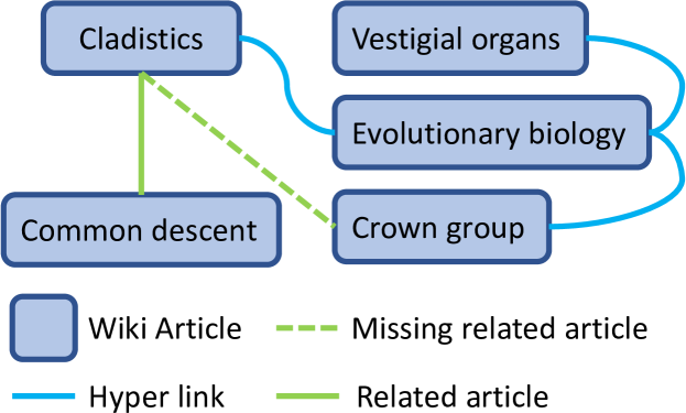
Figure 1. A snapshot from the LF-WikiSeeAlsoTitles-320K dataset for the article on “Cladistics”, a method of biological classification that groups organisms based on common ancestry, related article “Common descent” is tagged but the ground truth is incomplete and has missing labels such as “Crown group” which is refers to hierarchy of organisms. Traversal on hyperlink edges can help discover missing labels but must be used with caution since they can also lead to irrelevant labels such as “Vestigial organs”.

Although the use of textual and graph metadata can offer enhanced model accuracy in XC and recommendation settings (Yang et al., 2021; Mittal et al., 2021b; Saini et al., 2021; Chien et al., 2023), the use of GCN architectures makes both training and inference more expensive. It also requires the (bulky) graph to be preserved at inference time to embed a test data point which increases inference time and makes deployment challenging. These may be reasons behind the relatively limited adoption of graph metadata in XC literature and the focus on non-convolutional, text-only encoders such as DistilBERT, RoBERTA, etc.

Our Contributions: This paper develops RAMEN (gRaph regulArized encoder training for extreME classificatioN), a method to effectively utilize graph metadata at XC scales with minimal overheads in training cost and no overhead in model size or inference time. RAMEN can be incorporated into existing XC systems in a modular manner with few alterations. The key insights leading to RAMEN include a formal proof that in several use cases, GCN layers can be approximated by (much cheaper) non-GCN architectures and that it is more effective to use graph data to regularize encoder training than to implement a GCN. RAMEN can handle multiple graphs – graphs over data points, graphs over labels, or both – and offers increased prediction accuracy, even when presented with noisy graphs. RAMEN scales to datasets with up to 1M labels and can offer prediction accuracies that are up to 15% higher than state of the art methods including those that use graph metadata to train GCN. Code for RAMEN will be released publicly.

2. Related work

Extreme classification (XC) is a key paradigm in several areas such as ranking and recommendation. The literature on XC methods is vast (Dahiya et al., 2021a; Guo et al., 2019; Wydmuch et al., 2018; Zhang et al., 2018; Guo et al., 2019; Medini et al., 2019; Mittal et al., 2021a, b; Saini et al., 2021; Liu et al., 2017; You et al., 2019; Jiang et al., 2021; Chalkidis et al., 2019; Ye et al., 2020; Zhang et al., 2021; Mineiro and Karampatziakis, 2015; Babbar and Schölkopf, 2017; Jasinska et al., 2016; Khandagale et al., 2020; Jain et al., 2016; Prabhu et al., 2018a; Tagami, 2017; Yen et al., 2017; Wei et al., 2019; Siblini et al., 2018; Barezi et al., 2019; Jain et al., 2019; Gupta et al., 2019, 2023). Early XC methods used fixed (bag-of-words)  (Mineiro and Karampatziakis, 2015; Babbar and Schölkopf, 2017; Jasinska et al., 2016; Khandagale et al., 2020; Jain et al., 2016; Prabhu et al., 2018a; Tagami, 2017; Yen et al., 2017; Wei et al., 2019; Siblini et al., 2018; Barezi et al., 2019) or pre-trained (Jain et al., 2019) features and focused on learning only a classifier architecture. Recent advances have demonstrated significant gains by using task-specific features obtained from a variety of deep encoders such as bag-of-embeddings (Dahiya et al., 2021a, 2023b), CNNs (Liu et al., 2017), LSTMs (You et al., 2019), and transformers (Jiang et al., 2021; Chalkidis et al., 2019; Ye et al., 2020; Zhang et al., 2021). Training is scaled to millions of labels and training points (Dahiya et al., 2021a) by performing encoder pre-training followed by classifier training. A data point is trained only on its relevant labels (that are usually few in number) and a select few irrelevant labels deemed most informative using negative mining  (Mikolov et al., 2013; Dahiya et al., 2021b; Guo et al., 2019; Faghri et al., 2018; Chen et al., 2020; He et al., 2020a; Karpukhin et al., 2020; Lee et al., 2019; Luan et al., 2020; Hofstätter et al., 2021; Dahiya et al., 2023b; Xiong et al., 2021; Qu et al., 2021; Dahiya et al., 2023b).

Label Metadata in XC: Most XC methods use textual representation as label metadata since they allow scalable training and inference and allow leveraging good-quality pre-trained deep encoders such as RoBERTa (Liu et al., 2019a), DistilBERT base (Sanh et al., 2019), etc. Examples include encoder-only models such as TwinBERT (Lu et al., 2020) and ANCE (Xiong et al., 2021) and encoder+classifier architectures such as DECAF (Mittal et al., 2021a), SiameseXML (Dahiya et al., 2021b), X-Transformer (Chang et al., 2019), XR-Transformer (Chang et al., 2020), LightXML (Jiang et al., 2021), ELIAS (Zhang et al., 2021) and others (Ye et al., 2020; Liu et al., 2019b; You et al., 2019; Chalkidis et al., 2019). There is far less literature on the use of other forms of label metadata. For instance, ECLARE (Mittal et al., 2021b) and GalaxC (Saini et al., 2021) use graph convolutional networks whereas MUFIN (Mittal et al., 2022) explores multi-modal label metadata in the form of textual and visual descriptors for labels.

Graph Neural Networks in Related Areas: A sizeable body of work exists on using graph neural networks such as graph convolutional networks (GCN) for recommendation (Hamilton et al., 2018; Chen et al., 2018; Zou et al., 2019; Huang et al., 2018; Chiang et al., 2019; Zeng et al., 2020; Yang et al., 2021; Zhu et al., 2021; He et al., 2020b; Yang et al., 2022). Certain methods e.g., FastGCN (Chen et al., 2018), KGCL (Yang et al., 2022), LightGCN (He et al., 2020b) learn item embeddings as (functions of) free vectors. This makes it difficult for these methods to ingest novel items and their use is restricted to warm-start scenarios. Other GCN-based methods such as PINA (Chien et al., 2023), GraphSAGE (Hamilton et al., 2018) and GraphFormers (Yang et al., 2021) learn node representations as functions of node metadata e.g. textual descriptions. This allows the methods to work in zero-shot settings but they still incur the high storage and computational cost of GCNs. Moreover, diminishing returns are observed with increasing number of layers of the GCN (Chiang et al., 2019; Mittal et al., 2021b) with at least one model, namely LightGCN (He et al., 2020b) foregoing all non-linearities in its network, effectively opting for a single-layer GCN.

We now develop the RAMEN method that offers a far more scalable alternative to GCNs and other popular graph-based architectures in XC settings, significantly reducing the overheads of graph-based learning, yet offering sustained and significant performance boosts in prediction accuracies.

3. RAMEN: gRaph regulArized encoder training for extreME classificatioN

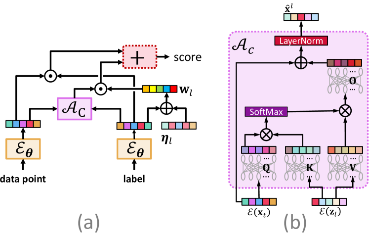
Figure 2. The model architecture adopted by RAMEN. A shared encoder is used to embed both data points and labels (a). A cross-attention architecture (b) is used to obtain a label-adapted representation of the data point, which is then scored by a classifier vector. This score is combined with the base label-datapoint similarity score to yield the final score.

Notation: Let $L$ be the total number of labels in the application. Note that the label set remains same across training and testing. Let ${{\mathbf{x}}}_{i},{{\mathbf{z}}}_{l}$ be the textual descriptions of the data point $i$ and label $l$ respectively. For each data point $i\in[N]$, its ground truth label vector is ${{\mathbf{y}}}_{i}\in\{-1,+1\}^{L}$, where $y_{il}=+1$ if label $l$ is relevant to the data point $i$ and otherwise $y_{il}=-1$. The training set is comprised of $N$ labeled data points and $L$ labels as ${\mathcal{D}}:=\{\{{{\mathbf{x}}}_{i},{{\mathbf{y}}}_{i}\}_{i=1}^{N},\{{{{\mathbf{z}}}_{l}}\}_{l=1}^{L}\}$. Let ${\mathcal{X}}\overset{\mathrm{def}}{=}\{{{\mathbf{x}}}_{i}\}_{i=1}^{N}$ denote the set of training data points and ${\mathcal{Z}}\overset{\mathrm{def}}{=}\{{{\mathbf{z}}}_{l}\}_{l=1}^{L}$ denote the set of labels. The meta-data graph over the auxiliary sets ${\mathcal{A}}$ (hyper-links, co-bidded queries) is denoted by ${\mathcal{G}}_{XA}$ and ${\mathcal{G}}_{ZA}$ for document and label respectively.

Metadata Graphs: RAMEN obtains metadata graphs over Anchor Sets. Let ${\mathcal{A}}=\left\{{{{\mathbf{a}}}_{1},{{\mathbf{a}}}_{2},\ldots,{{\mathbf{a}}}_{M}}\right\}$ denote an anchor set of $M$ elements. We abuse notation to let ${{\mathbf{a}}}_{m}$ denote the textual representation of anchor item $m\in[M]$ as well. Two distinct types of metadata graphs are possible over an anchor set:

1. Datapoint-anchor set: This is denoted as ${\mathcal{G}}_{XA}=(V_{XA},E_{XA})$ with $V_{XA}\overset{\mathrm{def}}{=}{\mathcal{X}}\cup{\mathcal{A}}$ i.e., the union of training data points and anchor points. The matrix $E_{XA}=\left\{{e_{im}}\right\}\in\left\{{0,1}\right\}^{N\times M}$ encodes whether data point ${{\mathbf{x}}}_{i}$ has an edge to to anchor item ${{\mathbf{a}}}_{m}$ or not.

2. Label-anchor set: This is denoted as ${\mathcal{G}}_{ZA}=(V_{ZA},E_{ZA})$ with $V_{ZA}\overset{\mathrm{def}}{=}{\mathcal{Z}}\cup{\mathcal{A}}$ i.e. the union of labels and anchor points. The matrix $E_{ZA}=\left\{{e_{lm}}\right\}\in\left\{{0,1}\right\}^{L\times M}$ encodes whether label ${{\mathbf{z}}}_{l}$ has an edge to anchor item ${{\mathbf{a}}}_{m}$ or not.

We refer the reader to Section 4 for details of how the metadata graphs are constructed using random walks. RAMEN can work with multiple anchor sets as well. For instance, given two anchor sets ${\mathcal{A}}^{1}=\left\{{{{\mathbf{a}}}^{1}_{1},{{\mathbf{a}}}^{1}_{2},\ldots,{{\mathbf{a}}}^{1}_{M_{1}}}\right\}$ and ${\mathcal{A}}^{2}=\left\{{{{\mathbf{a}}}^{2}_{1},{{\mathbf{a}}}^{2}_{2},\ldots,{{\mathbf{a}}}^{2}_{M_{2}}}\right\}$, a total of 4 meta data graphs are possible as described above.

Intuition behind RAMEN: A popular way to incorporate graph information into XC and recommendation tasks is to take initial embeddings of a data point from some encoder and use a graph convolution step to obtain augmented embeddings for the data point. For example, let $X\in{\mathbb{R}}^{N\times D}=[{{\mathbf{x}}}_{1},\ldots,{{\mathbf{x}}}_{N}]^{\top}$ be the initial embeddings of the $N$ data points over which a graph with adjacency matrix $A\in[0,1]^{N\times N}$ is present. A typical layer in a GCN performs an operation of the form $\phi(AXW)\in{\mathbb{R}}^{N\times D}$ where $W\in{\mathbb{R}}^{D\times D}$ is a transformation matrix and $\phi:{\mathbb{R}}\rightarrow{\mathbb{R}}$ is some activation function applied coordinate-wise. Not only is this step expensive (Zeng et al., 2020; Hamilton et al., 2018), but also offers diminishing returns with increasing number of layers (Chiang et al., 2019; Mittal et al., 2021b). Theorem 1 indicates that in cases where the adjacency matrix can be well-predicted using a non-GCN network (say feedforward or transformer) over the initial features, the convolutional layer can be well approximated by a non-GCN network as well. Note that edge prediction is often possible with high accuracy since the metadata graph available is closely linked to the prediction task at hand and Table 9 confirms this for the tasks considered in this paper. RAMEN uses this result to infer that it may be less useful to perform graph convolutions on top of a reasonably powerful encoder such as a transformer. Instead, utilizing the graph for regularization is cheaper yet effective. Theorem 1 is specified and proved in Appendix C in supplementary material. Extensions of Theorem 1 to networks with multiple GCN layers are also discussed.

Theorem 1 (Informal).

Let there exist a non-GCN (e.g. feedforward, transformer etc) network ${\mathcal{F}}:{\mathcal{X}}\rightarrow S^{P-1}$ where $S^{P-1}$ is the the unit sphere in say, $P$ dimensions, that effectively predicts edges in the metadata graph, say for any $i,j\in[N],a_{ij}\approx(1+{\mathcal{F}}({{\mathbf{x}}}_{i})^{\top}{\mathcal{F}}({{\mathbf{x}}}_{j}))/2$ where $A=[a_{ij}]$ is the adjacency matrix of the graph, then there exists another non-GCN network ${\mathcal{H}}$ such that $\phi(AXW)\approx[{\mathcal{H}}({{\mathbf{x}}}_{1}),\ldots,{\mathcal{H}}({{\mathbf{x}}}_{N})]^{\top}$.

Model Architecture: RAMEN’s architecture consists of three main components, encoder block (${\mathcal{E}}_{\boldsymbol{\theta}}$), cross-attention block (${\mathcal{A}}_{c}$) and extreme classifiers (${{\mathbf{w}}}$). The ${\mathcal{E}}_{\boldsymbol{\theta}}:{\mathcal{X}}\rightarrow{\mathcal{S}}^{D-1}$ with trainable parameters $\boldsymbol{\theta}$ is used to embed data points and labels using their textual descriptions. ${\mathcal{S}}^{D-1}$ denotes the $D$-dimensional unit sphere, i.e., the encoder provides unit norm embeddings. We will often use ${\mathcal{E}}(\cdot)$ to denote the encoder. RAMEN uses a DistilBERT base (Sanh et al., 2019) encoder as ${\mathcal{E}}$. RAMEN trains a cross-attention block ${\mathcal{A}}_{c}$ to learn label-adapted representations for data points. Specifically, given the embeddings of a data point ${\mathcal{E}}({{\mathbf{x}}})$ and a label ${\mathcal{E}}({{\mathbf{z}}}_{l})$, the attention block uses a standard attention mechanism parameterized by four $D\times D$ matrices, namely ${{\mathbf{Q}}},{{\mathbf{K}}},{{\mathbf{V}}},{{\mathbf{O}}}$ and outputs an alternate data point embedding that is adapted to that label $\hat{{\mathbf{x}}}^{l}\overset{\mathrm{def}}{=}{\mathcal{A}}_{c}({\mathcal{E}}({{\mathbf{x}}}),{\mathcal{E}}({{\mathbf{z}}}_{l}))$ (see Figure 2 for details). Along with the cross attention block RAMEN uses an 1-vs-all-style classifier architecture as ${{\mathbf{W}}}\overset{\mathrm{def}}{=}\{{{\mathbf{w}}}_{l}\}_{l\in[L]}$ where ${{\mathbf{w}}}_{l}$ is the classifier for label $l$ to rank the labels.

Metadata Graph Regularizers: Given an anchor set ${\mathcal{A}}$ and graphs ${{\mathbf{G}}}_{XA},{{\mathbf{G}}}_{ZA}$, we define the following two regularization functions over the encoder parameters:

(1) $${\mathcal{R}}_{x}(\boldsymbol{\theta}) =\textstyle\sum\limits_{i=1}^{N}\sum\limits_{\begin{subarray}{c}p:e_{ip}=1\\ n:e_{in}=0\end{subarray}}[{\mathcal{E}}_{\boldsymbol{\theta}}({{\mathbf{x}}}_{i})^{\top}{\mathcal{E}}_{\boldsymbol{\theta}}({{\mathbf{a}}}_{n})-{\mathcal{E}}_{\boldsymbol{\theta}}({{\mathbf{x}}}_{i})^{\top}{\mathcal{E}}_{\boldsymbol{\theta}}({{\mathbf{a}}}_{p})+\gamma]_{+}$$

(2) $${\mathcal{R}}_{z}(\boldsymbol{\theta}) =\textstyle\sum\limits_{l=1}^{L}\sum\limits_{\begin{subarray}{c}p:e_{lp}=1\\ n:e_{ln}=0\end{subarray}}[{\mathcal{E}}_{\boldsymbol{\theta}}({{\mathbf{z}}}_{l})^{\top}{\mathcal{E}}_{\boldsymbol{\theta}}({{\mathbf{a}}}_{n})-{\mathcal{E}}_{\boldsymbol{\theta}}({{\mathbf{z}}}_{l})^{\top}{\mathcal{E}}_{\boldsymbol{\theta}}({{\mathbf{a}}}_{p})+\gamma]_{+}$$

Here, $p$ is the positive anchor and $n$ are in-batch negatives anchors (explained in later section). Note that these two regularizers encourage the encoder to keep data points and labels closely embedded to their related anchor points and far away from unrelated anchor points. If we have more than one anchor set, say ${\mathcal{A}}^{1},{\mathcal{A}}^{2}$, we can define corresponding regularizers ${\mathcal{R}}^{t}_{x}(\boldsymbol{\theta}),{\mathcal{R}}^{t}_{z}(\boldsymbol{\theta}),t{=}1,2$.

RAMEN Training: RAMEN performs modular training involving two modules. In the first module the encoder is pre-trained all by itself. Then the encoder is fixed and the classifiers and cross-attention block are jointly trained in the second module. The details of the two modules are given below. Hyperparameter tuning is discussed in Section 4.

Module M1 (Encoder Training): Encoder is trained using Document-label loss (${\mathcal{L}}(\boldsymbol{\theta})$) regularized using two components: a) anchor set on document side (${\mathcal{R}}_{x}(\boldsymbol{\theta})$) and b) anchor sent on label side (${\mathcal{R}}_{z}(\boldsymbol{\theta})$) as discussed in the previous section. The ${\mathcal{L}}(\boldsymbol{\theta})$ function takes the following formulation:

$${\mathcal{L}}(\boldsymbol{\theta})=\sum_{i=1}^{N}\sum_{\begin{subarray}{c}l:y_{il}=+1\\ k:y_{ik}=-1\end{subarray}}[{\mathcal{E}}_{\boldsymbol{\theta}}({{\mathbf{z}}}_{k})^{\top}{\mathcal{E}}_{\boldsymbol{\theta}}({{\mathbf{x}}}_{i})-{\mathcal{E}}_{\boldsymbol{\theta}}({{\mathbf{z}}}_{l})^{\top}{\mathcal{E}}_{\boldsymbol{\theta}}({{\mathbf{x}}}_{i})+\gamma]_{+},$$

Note that this loss function encourages the encoder to embed a data point close to its relevant labels and far from irrelevant ones. The encoder is trained by minimizing the following regularized objective

$$\min_{\boldsymbol{\theta}}\lambda_{l}\cdot{\mathcal{L}}(\boldsymbol{\theta})+\sum_{t=1,2}(\lambda^{t}_{x}\cdot{\mathcal{R}}^{t}_{x}(\boldsymbol{\theta})+\lambda^{t}_{z}\cdot{\mathcal{R}}^{t}_{z}(\boldsymbol{\theta}))$$

where $\lambda_{l},\lambda^{t}_{x},\lambda^{t}_{z}$ are regularization constants that are estimated using a bandit optimization strategy described below. This step can accommodate multiple anchor sets as well as regularizers.

Bandit Learning for Regularization Constants: The simple gradient descent without a gradient approach (Flaxman et al., 2005) was adopted to tune the regularization constants $\lambda_{l},\lambda_{t,x},\lambda_{t,z}$ in an online manner. $\lambda_{l}$ was initialized to 1 and $\lambda_{t,x},\lambda_{t,z}$ to 0.1. Below we describe the process for a single constant $\lambda$ and the same is independently replicated for all the constants.

After every 30 iterations, the value of lambda is perturbed as $\hat{\lambda}=\lambda+z,z\sim{\mathcal{N}}(0,0.01)$, where ${\mathcal{N}}(0,0.01)$ denotes a unidimensional Gaussian with zero mean and variance 0.01. Then $\hat{\lambda}$ is used as the regularization constant in the loss expression for the next 30 iterations. The mini-batch objective values ($\lambda_{l}\cdot{\mathcal{L}}+\sum_{t=1,2}(\lambda^{t}_{x}\cdot{\mathcal{R}}^{t}_{x}+\lambda^{t}_{z}\cdot{\mathcal{R}}^{t}_{z})$) incurred in these 30 iterations is calculated as say $P$. Afterward, $\lambda$ is updated using an estimated gradient as follows

$$\lambda=\lambda-\eta\cdot\frac{P}{\hat{\lambda}-\lambda},$$

where $\eta$ is a learning rate. This is justified by a simple but surprising application of the Stokes theorem (Flaxman et al., 2005) that states that for any function $f:{\mathbb{R}}\rightarrow{\mathbb{R}}$ (which can itself be non-convex or even non-differentiable), we have $\frac{d\hat{f}(x)}{dx}=\frac{1}{\delta}\cdot\underset{u\sim\left\{{-1,+1}\right\}}{{\mathbb{E}}}\left[{{f(x+\delta u)u}}\right]$ where $\hat{f}:{\mathbb{R}}\rightarrow{\mathbb{R}}$ is a smoothed version of $f$ defined as $\hat{f}(x)\overset{\mathrm{def}}{=}\underset{v\sim[-1,1]}{{\mathbb{E}}}\left[{{f(x+\delta v)}}\right]$. Note $\hat{f}$ is always differentiable even if $f$ is not. In order to compute mini-batch objectives, $P$, RAMEN mines hard negatives. The negative mining technique is explained below.

Negative Mining: The loss function and regularizers contain ${\mathcal{O}}\left({{NL\log L+(N+L)M\log M}}\right)$ terms where $M=\max\left\{{M_{1},M_{2}}\right\}$ is the maximum number of anchors in any of the anchor sets. This is because the number of relevant labels per data point is usually limited by $|l:y_{il}=+1|\leq{\mathcal{O}}\left({{\log L}}\right)$ in XC applications (Jain et al., 2016) and we can construct the metadata graphs to have at most $\log M$ relevant anchors per data point or label. Performing optimization with respect to all these terms is expensive which is why RAMEN utilizes in-batch negative mining (Dahiya et al., 2023b; Chen et al., 2020; Dahiya et al., 2021b; Faghri et al., 2018; Guo et al., 2019; He et al., 2020a). Specifically, a set of data points is identified and for each data point, a random relevant label and random related anchor is chosen (from each anchor set if there are multiple anchor sets). For the chosen labels a random related anchor is chosen from each anchor set. Then hard negative labels for a data point are chosen only among labels selected for this mini-batch. Similarly, hard negative anchors for a data point or label are chosen only among anchors selected for this mini-batch. Once the encoder is learned, the parameters are frozen and RAMEN learns extreme classifiers in module 2 which is explained next.

Module M2 (Cross Attention and Classifier Training): Once the encoder is trained, it is frozen and a maximum inner product search (MIPS) data structure is established over the label embeddings ${\mathcal{E}}({{\mathbf{z}}}_{l}),l\in[L]$. For each training data point $i\in[N]$, a set of $100\approx\log L$ labels with the highest label similarity score ${\mathcal{E}}_{\boldsymbol{\theta}}({{\mathbf{z}}}_{l})^{\top}{\mathcal{E}}_{\boldsymbol{\theta}}({{\mathbf{x}}}_{i})$ by firing MIPS queries. This returns a shortlist $\hat{\mathcal{N}}_{i}\subset[L]$ of labels for each data point. Relevant labels present in this set are removed so that $y_{ik}=-1$ for all $k\in\hat{\mathcal{N}}_{i}$. Next, the classifiers ${{\mathbf{w}}}_{l},l\in[L]$ and attention block parameters ${{\mathbf{Q}}},{{\mathbf{K}}},{{\mathbf{V}}},{{\mathbf{O}}}$ are trained. The classifiers are initialized to ${{\mathbf{w}}}_{l}\overset{\mathrm{init}}{\leftarrow}{\mathcal{E}}({{\mathbf{z}}}_{l})$. Training is done by minimizing the triplet loss function:

(3) $${\mathcal{L}}(\left\{{{{\mathbf{w}}}_{l}}\right\}_{l\in[L]},{{\mathbf{Q}}},{{\mathbf{K}}},{{\mathbf{V}}},{{\mathbf{O}}})=\textstyle\sum_{i=1}^{N}\sum_{\begin{subarray}{c}l:y_{il}=+1\\ k:y_{ik}=-1\end{subarray}}[{{\mathbf{w}}}_{k}^{\top}\hat{{\mathbf{x}}}_{i}^{k}-{{\mathbf{w}}}_{l}^{\top}\hat{{\mathbf{x}}}_{i}^{l}+\gamma]_{+},$$

where $\hat{{\mathbf{x}}}^{l}\overset{\mathrm{def}}{=}{\mathcal{A}}_{c}({\mathcal{E}}({{\mathbf{x}}}),{\mathcal{E}}({{\mathbf{z}}}_{l}))$ is the label-adapted embedding for the data point $i$ with respect to label $l$ (see Figure 2 for details). Note that equivalently, we could have parameterized the classifier as ${{\mathbf{w}}}_{l}={\mathcal{E}}({{\mathbf{z}}}_{l})+\boldsymbol{\eta}_{l}$, initialized $\boldsymbol{\eta}_{l}={\mathbf{0}}$ and trained $\boldsymbol{\eta}_{l}$ instead by minimizing ${\mathcal{L}}(\left\{{\boldsymbol{\eta}_{l}}\right\}_{l\in[L]},{{\mathbf{Q}}},{{\mathbf{K}}},{{\mathbf{V}}},{{\mathbf{O}}})$. Figure 2 uses this parameterization of the classifier to emphasize the initialization. Also note that negative mining is not needed in this module since training is already done with respect to a shortlist of negative labels leaving us with just ${\mathcal{O}}\left({{N\log^{2}L}}\right)$ terms in total.

Inference with RAMEN: Given a test point ${{\mathbf{x}}}_{t}$, its embedding ${\mathcal{E}}({{\mathbf{x}}}_{t})$ is computed and used to fire a MIPS query to retrieve a set $\hat{\mathcal{N}}_{t}$ of the $100\leq{\mathcal{O}}\left({{\log L}}\right)$ labels with the highest label similarity score i.e. $s^{s}_{tl}\overset{\mathrm{def}}{=}{\mathcal{E}}_{\boldsymbol{\theta}}({{\mathbf{z}}}_{l})^{\top}{\mathcal{E}}_{\boldsymbol{\theta}}({{\mathbf{x}}}_{t}),l\in\hat{\mathcal{N}}_{t}$. Next, for each of these labels, the label adapted embedding of the test point is calculated for each shortlisted label ${{\mathbf{x}}}^{l}_{t}\overset{\mathrm{def}}{=}{\mathcal{A}}_{c}({\mathcal{E}}({{\mathbf{x}}}_{t}),{\mathcal{E}}({{\mathbf{z}}}_{l})),l\in\hat{\mathcal{N}}_{t}$. Then the classifier score is computed as $s^{c}_{tl}\overset{\mathrm{def}}{=}{{\mathbf{w}}}_{l}^{\top}{{\mathbf{x}}}^{l}_{t},l\in\hat{\mathcal{N}}_{t}$. The classifier and similarity scores are then combined linearly as $s_{tl}=\beta\cdot s^{c}_{tl}+(1-\beta)\cdot s^{s}_{tl}$. A fixed value of $\beta=0.7$ was used. Final predictions are made in descending order of the scores $s_{tl}$. RAMEN performs predictions in time ${\mathcal{O}}\left({{B+D\log L}}\right)$ where $B=|\boldsymbol{\theta}|$ is the size of the encoder architecture and $D$ is the embedding dimensionality. In practice, RAMEN offers predictions within 4 milliseconds. It is notable that even though RAMEN uses a graph at training time, inference does not require the bulky graph, making it highly suitable for large-scale applications.

Table 1. Results on short-text benchmark datasets. RAMEN is up to 15% more accurate as compared to both text-based and graph-based baselines. RAMEN-M1 indicates accuracies obtained after module M1 i.e. without training the classifier and cross-attention architecture to offer a fair comparison to other methods that do not adopt a classifier. Note that including the classifier and cross-attention architecture offers a 2.5 – 4.5% improvement in P@1.

PSP@1 PSP@3 PSP@5 PSN@3 PSN@5 P@1 P@3 P@5 N@3 N@5 LF-WikiSeeAlsoTitles-320K RAMEN-M1 26.66 28.68 30.85 29.11 30.85 32.17 21.57 16.33 32.16 33.26 NGAME-M1 25.14 26.77 28.73 27.27 28.86 30.79 20.34 15.36 30.47 31.45 GraphSage 21.56 21.84 23.5 22.93 24.57 27.3 17.17 12.96 27.1 28.36 GraphFormer 19.24 20.64 22.7 20.98 22.68 21.94 15.1 11.79 22.61 24.02 RAMEN 26.96 29.8 32.55 30.00 32.06 33.95 23.15 17.7 34.2 35.54 NGAME 24.41 27.37 29.87 27.39 29.21 32.64 22 16.6 32.3 33.21 DEXA 24.45 26.52 28.62 26.97 28.6 31.71 21.03 15.84 31.34 32.29 ELIAS 13.47 15.88 17.69 15.57 16.85 23.36 15.64 11.85 22.86 23.62 CascadeXML 12.68 15.37 17.63 14.65 16.05 23.39 15.71 12.06 22.6 23.43 XR-Transformer 10.6 11.78 12.72 11.7 12.44 19.44 12.25 8.98 18.26 18.53 AttentionXML 9.45 10.63 11.73 10.45 11.24 17.56 11.34 8.52 16.58 17.07 SiameseXML 26.82 28.42 30.36 28.74 30.27 31.97 21.43 16.24 31.57 32.59 ECLARE 22.01 24.23 26.27 24.46 26.03 29.35 19.83 15.05 29.21 30.2 DECAF 16.73 18.99 21.01 19.18 20.75 25.14 16.9 12.86 24.99 25.95 Parabel 9.24 10.65 11.8 10.49 11.32 17.68 11.48 8.59 16.96 17.44 Bonsai 10.69 12.44 13.79 12.29 13.29 19.31 12.71 9.55 18.74 19.32 LF-WikiTitles-500K RAMEN-M1 28.31 26.25 25.23 28.87 30.35 44.92 24.9 17.04 34.69 33.06 NGAME-M1 23.18 22.08 21.18 24.51 26.05 29.68 18.06 12.51 25.4 25.1 GraphSage 22.35 19.31 19.15 22.09 23.82 27.19 15.66 11.3 22.6 22.78 GraphFormer 22.04 19.2 19.53 21.29 22.78 24.53 14.92 11.33 20.23 20.35 RAMEN 27.61 26.89 26.02 29.15 30.7 47.12 26.86 18.55 36.88 35.1 NGAME 23.12 23.31 23.03 25.34 27.22 39.04 23.1 16.08 31.8 30.75 CascadeXML 19.19 19.47 19.75 20.8 22.34 47.29 26.77 19 36.19 34.36 AttentionXML 14.8 13.97 13.88 15.24 16.22 40.9 21.55 15.05 29.38 27.45 ECLARE 21.58 20.39 19.84 22.39 23.61 44.36 24.29 16.91 33.33 31.46 DECAF 19.29 19.82 19.96 21.26 22.95 44.21 24.64 17.36 33.55 31.92 Bonsai 16.58 16.34 16.4 17.6 18.85 40.97 22.3 15.66 30.35 28.65 LF-AmazonTitles-1.3M RAMEN-M1 36.61 39.66 41.03 39 40.24 47.78 42.14 37.74 46.48 45.54 NGAME-M1 33.03 35.63 36.8 - - 45.82 39.94 35.48 - - GraphSage 24.54 24.16 23.72 24.66 24.89 28.13 21.43 17.58 24.79 23.17 GraphFormer 22.53 22.4 22.55 22.59 23.07 24.19 17.43 14.26 21.59 20.84 RAMEN 34.44 38.42 40.47 37.7 39.52 55.67 49.66 44.66 54.44 53.39 NGAME 29.18 33.01 35.36 32.07 33.9 56.75 49.19 44.09 53.84 52.41 DEXA 29.12 32.69 34.86 32.02 33.86 56.63 49.05 43.9 53.81 52.37 CascadeXML 17.17 21.7 24.76 19.86 21.51 47.82 42.05 38.31 45.01 43.77 XR-Transformer 20.06 24.85 27.79 23.44 25.41 50.14 44.07 39.98 47.71 46.59 PINA - - - - - 55.76 48.70 43.88 - - AttentionXML 15.97 19.9 22.54 18.23 19.6 45.04 39.71 36.25 42.42 41.23 SiameseXML 27.12 30.43 32.52 29.41 30.9 49.02 42.72 38.52 46.38 45.15 ECLARE 23.43 27.9 30.56 26.67 28.61 50.14 44.09 40 47.75 46.68 DECAF 22.07 26.54 29.3 25.06 26.85 50.67 44.49 40.35 48.05 46.85 Parabel 16.94 21.31 24.13 19.7 21.34 46.79 41.36 37.65 44.39 43.25 Bonsai 18.48 23.06 25.95 21.52 23.33 47.87 42.19 38.34 45.47 44.35

Table 2. Results on full-text benchmark datasets. RAMEN is up to 15% more accurate as compared to both text-based and graph-based baselines. RAMEN-M1 indicates accuracies obtained after module M1 i.e. without training the classifier and cross-attention architecture to offer a fair comparison to other methods that do not adopt a classifier. Note that including the classifier and cross-attention architecture offers up to 6% and 4% improvement in PSP@1 and P@1 respectively.

PSP@1 PSP@5 PSN@5 P@1 P@5 N@5 LF-WikiSeeAlso-320K RAMEN-M1 34.38 41.6 42.02 47.29 23.37 49.15 NGAME-M1 29.6 32.83 34.19 45.65 17.32 45.43 GraphSage 20.56 23.07 26.57 24.14 9.08 25.28 GraphFormer 16.85 20.98 20.41 18.14 8.81 20.81 RAMEN 33.81 41.77 41.95 48.21 23.88 49.97 NGAME 28.18 33.33 34.01 46.4 18.05 46.64 DEXA 31.81 38.78 - 47.11 22.71 47.62 CascadeXML 22.26 31.1 28.87 40.42 20.2 40.55 XR-Transformer 25.18 33.79 32.59 42.57 21.3 43.44 PINA - - - 44.54 22.92 - AttentionXML 22.67 29.83 28.38 40.5 19.87 40.26 LightXML 17.85 24.16 22.8 34.5 16.83 34.24 SiameseXML 29.02 36.03 35.17 42.16 21.39 43.36 ECLARE 26.04 33.01 32.32 40.58 20.14 41.23 DECAF 25.72 34.89 33.69 41.36 21.38 43.32 Parabel 17.1 23.53 21.88 33.46 16.61 33.34 Bonsai 18.19 25.66 23.84 34.86 17.66 35.32 LF-Wikipedia-500K RAMEN-M1 50.94 61.94 61.84 81.07 50.1 75.27 NGAME-M1 50.99 57.33 - 77.92 40.95 - GraphSage 35.21 37.75 40.76 43.14 28.32 35.32 GraphFormer 25.16 21.83 24.83 31.1 14 24.87 RAMEN 43.63 61.77 60.15 85.98 52.56 79.23 LEVER 42.50 60.20 - 85.02 52.02 - DecoupledSoftmax - 58.97 - 85.78 50.53 77.11 NGAME 41.25 57.04 56.11 84.01 49.97 75.97 DEXA 42.59 58.33 57.44 84.92 50.51 76.8 ELIAS 35.02 51.13 - 81.26 48.82 73.1 CascadeXML 31.87 44.89 43.87 80.69 46.25 70.49 XR-Transformer 33.58 47.81 46.61 81.62 47.85 72.43 PINA - - - 82.83 50.11 - AttentionXML 34 50.15 47.69 82.73 50.41 74.86 LightXML 31.99 46.53 45.18 81.59 47.64 72.23 SiameseXML 33.95 37.07 38.93 67.26 33.73 54.29 ECLARE 31.02 38.29 34.5 68.04 35.74 56.37 Parabel 26.88 35.26 34.61 68.7 38.64 58.62 Bonsai - - - 69.2 38.8 -

Table 3. Results on the proprietary dataset (G-EPM-1M). RAMEN is up to 10% more accurate than the leading method NGAME which is also RAMEN’s closest competitor on public datasets.

PSP@1 PSP@3 P@1 P@5 R@10 RAMEN 25.13 47.2 25.18 9.81 55.93 NGAME 16.23 31.5 15.07 6.26 37.22

4. Experiments

The XML Repository (Bhatia et al., 2016) provides various public XC datasets which are thoroughly studied and benchmarked by plethora of papers. These datasets are curated from Wiki dumps link and Amazon dump (Ni et al., 2019) but metadata, which was readily available, was ignored. RAMEN crawel these dumps and curated meta data for all public datasets. The details are as follows:

LF-WikiSeeAlsoTitles-320K: The dataset was curated from Wiki dump link. The scenario involved recommending related articles. Articles under the “See Also” section were used as ground truth labels. Internal hyperlinks and category links were used to create two sets of metadata graphs, one using Wikipedia articles as anchors and the other using Wikipedia categories as anchors. For the additional full text version (LF-WikiSeeAlso-320K), first 128 words in the main text were used along with page title for the document.

LF-WikiTitles-500K: The dataset was also curated from Wiki dump link. The scenario involved recommending relevant “categories” for an article. Internal hyperlinks and category-to-category links were used to create two sets of metadata graphs as described above. For the additional full text version (LF-Wikipedia-500K), first 128 words in the main text were used along with page title for the document.

LF-AmazonTitles-1.3M: The dataset was curated from Amazon dump (Ni et al., 2019). The scenario involved recommending relevant “product” for a product. The “similar_items” links given in the data dump were used to create metadata graph.

G-EPM-1M: Matching user queries with relevant advertiser keywords is a critical component of sponsored search. One type of matching is Extended Phrase Match (EPM), which aims to match a user query with advertiser keywords that have a subset of the query’s intent. This means that only keywords with similar intent to the query are considered. For example, for the query "cheap nike shoes", a valid EPM keyword is "nike sneakers" but "adidas shoes" or "nike shorts" are not.

Maintaining this intent-subset requirement is challenging but important for advertisers who may bid differently on different match types for the same keyword. Improving the effectiveness of this matching process, particularly for less common queries and keywords, can enhance the search experience for users and benefit small advertisers such as mom-and-pop businesses. To study the effectiveness of RAMEN in this application, a dataset called G-EPM-1M was curated by analyzing the click logs of a popular search engine. The click logs were mined to gather graph metadata for RAMEN, including three types of signals:

1. Co-session queries: Queries that were asked in the same search session by multiple users.

2. Co-clicked queries: Queries that resulted in clicks on the same webpage.

3. Co-asked queries: Queries that were clicked in the "users also ask" section on the search engine in response to a specific query.

These metadata were collected over an extended period of time and used to provide additional information to RAMEN.

Dataset Statistics: Please refer to Tab. 10 in supplementary material for dataset statistics. For all datasets, test data points were removed from the graph if ever present as nodes to prevent train-test leaks.

Evaluation Metrics: For public datasets and offline proprietary tasks, standard evaluation metrics were used including recall@$k$ (R@$k$), precision@$k$ (P@$k$), nDCG@$k$ (N@$k$), their propensity scored variants (which give more weightage to accurate prediction of tail/rare labels) (Jain et al., 2016) and false-negatives@$k$ (FN@$k$). Note that predicting tail labels in more rewarding in real-world scenarios. Therefore, we focus on gains in propensity scored metrics. Please refer to Appendix B in the supplementary for definitions of these metrics. Instructions on the XML repository (Bhatia et al., 2016) were closely followed to ensure fair evaluation.

Implementation details: Links obtained on the metadata graph from raw data suffer from missing links in much the same way there are missing labels in the ground truth. To deal with this, RAMEN performs a random walk with restart on each anchor node. The random walk was performed for 400 hops with a restart probability of 0.8, thus ensuring that the walk did not wander too far from the starting node. This random walk could also introduce noisy edges, leading to poor model performance. To deal with such edges, in-batch pruning was performed and edges to only those anchors were retained which had a cosine similarity of $>0$ based on the embeddings given the encoder. To get the encoder, RAMEN initialize the encoder with a pre-trained DistilBERT and fine-tuned it for 10 epochs(warmup phase) using unpruned metadata graphs. Then the metadata graphs were pruned using the fine-tuned encoder. Encoder fine-tuning was then was continued for 5 epochs using the pruned graphs after which the graphs were re-pruned. These alternations of 5 epochs of encoder fine-tuning followed by re-pruning were repeated till convergence. The learning rate for each bandit was set to $0.001$. Table 11 in supplementary material summarizes all hyper-parameters for each dataset. It is notable that even though RAMEN uses a graph at training time, inference does not require any such information, making it highly suitable for long-tail queries. RAMEN uses the PyTorch (Paszke et al., 2017) framework and model on each benchmark datasets and was trained on $2\times$ Nvidia V100 GPUs.

Results on benchmark datasets: Table 1 compares RAMEN with graph and XC methods. RAMEN can be up to 5% more accurate over the best baseline numbers. In particular RAMEN can be 16% more accurate than traditional graph-based methods. Additionally, RAMEN can be 3-4% more accurate over PINA (Chien et al., 2023), which uses both XC and same anchor sets with the encoder 2$\times$ that of RAMEN. Figure 3 shows that RAMEN outperforms baseline methods in each quantile, showing its overall superior embedding quality. RAMEN’s improvement in all quantiles can also be attributed to the fact that RAMEN can make correct predictions on head and tail alike compared to baselines which focused mostly on the tail as indicated by the t-SNE plot in figure 4. RAMEN outperforms baseline methods on all datasets however, low gains in LF-AmazonTitles-1M can be attributed the low volume of metadata (“similar_items” graph edges) available for training (ref to Table 10 in supp. material). Please refer to ablation study section where we show that lower volume of metadata leads to lower gains. Note that, RAMEN’s primary focus is short-text documents but RAMEN is also state-of-the-art in full text counter parts of the dataset (Table 2).

Table 4 shows that RAMEN could make predictions such as “Crown group” which were missing labels in the training, by exploiting metadata graph links. Apart from standard metrics, the error rate plays a crucial role in deployment. Tab. 4 compares the difference in RAMEN’s false negative rate ($\text{FN}@k$) with the best-performing baseline (NGAME) when each method was allowed to make $k$ predictions i.e., $\text{Diff}@k\overset{\mathrm{def}}{=}\text{FN}@k$(RAMEN) - $\text{FN}@k$(NGAME). It is notable that RAMEN consistently outperforms NGAME over all label quantiles (i.e. over head/popular as well as tail/rare labels) and performs even better at higher values of $k$ such as $k=50$.

Table 4. A subjective comparison of predictions made by RAMEN, the leading text-based method NGAME, and the leading graph-based method GraphFormers on LF-WikiSeeAlsoTitles-320K. Labels that are a part of the ground truth are formatted in black color. Labels not a part of the ground truth are formatted in light gray color. Relevant labels that are missing from the ground truth are marked in bold black. RAMEN could make predict highly relevant labels such as “Crown group”, which were missing from the ground truth as well as omitted by other methods.

Method	Prediction
Document: Clade
RAMEN	Cladistics, Phylogenetics, Crown group, Paraphyly, Polyphyly
NGAME	Cladistics, Linnaean taxonomy, Polyphyly, Paragroup, Molecular phylogenetics
GraphFormers	SUPERFAMILY, Phylogenetic network, Phylogenetics Phylogenetic tree, Phylogeny

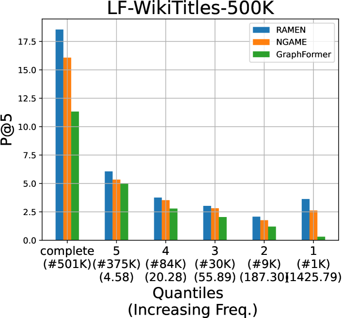
Figure 3. Quantile wise-comparison of RAMEN and other methods. RAMEN gives consistent gains in each bin (see Appendix B for binning details). The left-most bin contains the most rare/tail labels whereas the rightmost bin contains the most popular/head labels.

Table 5. Comparing the difference in false negative rates between RAMEN and NGAME on LF-WikiSeeAlsoTitles-320K. Results are presented in a quantile-wise manner. The #5K label quantile contains the most popular/head labels whereas the #729K quantile contains the most rare/tail labels. See Appendix B for definitions of metrics and quantiles. RAMEN’s false negative rate is always superior to that of NGAME but the gap widens significantly when compared on tail labels.

Quantile (#L) Avg. Doc.	DIFF@5	DIFF@10	DIFF@20	DIFF@50	DIFF@100
(#1K) 200.78	-0.019	-0.026	-0.027	-0.021	-0.010
(#9K) 30.98	0.013	-0.050	-0.107	-0.123	-0.049
(#31K) 9.14	0.036	-0.124	-0.272	-0.443	-0.423
(#74K) 3.94	-0.455	-0.757	-1.091	-1.551	-1.854
(#195K) 1.49	-2.246	-2.722	-3.529	-4.763	-6.075
complete	-2.671	-3.679	-5.025	-6.901	-8.411

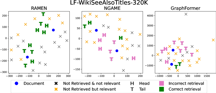
Figure 4. t-SNE of retrieved labels of document “terrestrial locomotion” and “Cladistics” by RAMEN, NGAME, GraphFormers. RAMEN has a much higher number of correct retrievals and retrieves a healthy mix of both head (H) and tail (T) labels, while other methods retrieve far fewer relevant labels and focus on predicting tail labels.

Results on proprietary datasets: Table 3 compares RAMEN against NGAME on the G-EPM-1M dataset. RAMEN was found to be 3% better on the P@5 metric. RAMEN was further found to be 15% better than NGAME on the propensity scored PSP@5 metric, indicating that RAMEN could match tail keywords more accurately. The quality of the two models was further measured using an in-production, large cross-encoder oracle quality model that was trained on an extensive set of manually labeled data. The oracle quality model found predictions made by RAMEN to be 43% more accurate than those made by NGAME.

Ablation: Experiments were conducted to understand the impact of the design choices made by RAMEN as well as the impact of metadata on the performance of RAMEN. Table 6 complies these experiments. In particular, experiment “No-Bandits” explored the effects of different choices of giving weights to different sources of metadata on RAMEN’s performance. A key finding was that when uniform weights were assigned to all graphs, there was a substantial 18% drop in P@1. This highlights the importance of bandit learning, where each graph’s contribution is determined dynamically. To understand the impact of noisy edges in metadata, experiment "No Pruning" disabled the trimming of noisy edges using cosine similarity filtering. A 1.5% loss in P@1 was observed which underscores the necessity of pruning unhelpful edges during training to maintain high performance.

RAMEN uses multiple meta-data graphs for both document and label. To ascertain the contributions of the anchor-doc and anchor-label metadata graphs, the ablations "No Doc. Graph" and "No Lbl. Graph" were conducted. These experiments reveal that information from these graphs plays a significant role, as disabling either leads to a 1.5–2% reduction in P@1. The information from these graphs can be incorporated in baseline methods like NGAME. To understand its impact, experiment “AugGT’ trains NGAME with augmented ground truth. The ground truth was expanded by using label propagation wherein a label is given an edge to a training point if the label shares a neighbor in the metadata graph with said training point. RAMEN outperformed the “AugGT” setup by 15%. This suggests that while leveraging graph information for ground truth enhancement is convenient, it may not be as effective due to noisy edges.

Further Analysis: RAMEN’s robust training strategy extends benefits beyond its own performance. SiameseXML and ECLARE, baseline methods, experienced improvements of 3% and 5% in P@1, respectively, when leveraging RAMEN’s metadata regularizer (Table 7). Further experiments on the LF-WikiSeeAlsoTitles-320K dataset evaluate the influence of metadata volume. Reducing metadata to 50% and 20% results in performance drops of 1–2.5% in propensity scored precision and 3–4% in precision. This emphasizes the importance of metadata in enhancing performance, particularly for tail labels (Table 8). Additionally RAMEN can predict meta-data graph links with high accuracy (Table 9) and therefore validate the proposed theorem 1.

These experiments collectively shed light on the intricate interplay between design choices and metadata utilization, underscoring the effectiveness and nuances of RAMEN’s approach.

Table 6. Ablations were done on module M1 (RAMEN-M1) on LF-WikiSeeAlsoTitles-320K to understand the impact of design choices on the quality of encoder training. RAMEN’s design choices are seen to be optimal and offer 2.5–13% improvement in the P@1 metric over alternate design choices.

RAMEN P@1 P@3 P@5 N@3 N@5 RAMEN-M1 32.17 21.57 16.33 32.16 33.26 $-$ No Bandits 20.91 12.81 9.53 21.46 22.5 $-$ No Pruning 31.31 18.94 12.8 31.43 31.51 $-$ No Doc. Graph 29.73 17.46 12.5 30.71 30.8 $-$ No Lbl. Graph 28.53 17.73 12.61 31.04 32.06 AugGT 15.56 8.95 6.48 15.67 16.32

Table 7. Results of RAMEN as a regularizer in baseline algorithms on LF-WikiSeeAlsoTitles-320K. RAMEN’s regularization algorithm improves the performance of the base algorithm by 1–2%

P@1 P@3 P@5 N@3 N@5 RAMEN 33.95 23.15 17.7 34.2 35.54 SiameseXML 31.97 21.43 16.24 31.57 32.59 + RAMEN 32.01 21.89 17.59 31.74 32.92 ECLARE 29.35 19.83 15.05 29.21 30.2 + RAMEN 30.53 20.11 16.42 32.33 32.83

Table 8. Impact of metadata on the performance of RAMEN on LF-WikiSeeAlsoTitles-320K. RAMEN’s performance on P and PSP decreases as we decrease the volume of metadata.

PSP@1 PSP@5 P@1 P@5 RAMEN 26.96 32.55 33.95 17.7 RAMEN (20%) 25.8 30.12 31.08 15.98 RAMEN (50%) 26.37 31.11 31.68 16.44

Table 9. RAMEN’s encoder ${\mathcal{E}}$ can predict links in the meta-data graph with extremely high recall (R@100).

Link type	LF-WikiSeeAlsoTitles-320K	LF-WikiTitles-500K
hyper_link	99.88	94.20
category	99.88	99.96

5. Conclusion

This paper presented RAMEN, a novel approach for leveraging metadata to enhance the accuracy of recommendation systems w.r.t. rare labels. A key takeaway from the study is that opting for graph-based regularization instead of the more prevalent GCN architectures, can yield gains of up to 15% in PSP@1/P@1 compared to graph-based methodologies, and up to 6% when compared with XC techniques tailored for recommendation systems. The bandit-style regularization technique adopted by RAMEN was found to offer performance boosts to RAMEN as well as other baseline methods and can be of independent interest. Notably, RAMEN offers state-of-the-art performance without incurring any computational overhead during inference.

6. Ethical Considerations

Our usage of data and terms of providing service to people around the world has been approved by our legal and ethical boards. In terms of social relevance, our research is helping millions of people find the goods and services that they are looking for online with increased efficiency and a significantly improved user experience. This facilitates purchase and delivery without any physical contact which is important given today’s social constraints. Furthermore, our research is increasing the revenue of many small and medium businesses including mom and pop stores while also helping them grow their market and reduce the cost of reaching new customers.

Graph Regularized Encoder Training for Extreme Classification
(Appendix)

Appendix A Data stats

Table 10. Dataset statistics summary for benchmark datasets used by RAMEN. Entries marked with $\ddagger$ were not disclosed because the dataset is proprietary.

# Train Pts $N$ # Labels $L$ # Test Pts $N^{\prime}$ Avg. docs. per label Avg. labels per doc. Graph Types # Graph Nodes $G$ Avg. node neighbors per doc. Avg. node neighbors per label LF-WikiSeeAlsoTitles-320K / LF-WikiSeeAlso-320K 693,082 312,330 177,515 4.67 2.11 Hyperlink Category 2,458,399 656,086 38.87 4.74 7.71 4.82 LF-WikiTitles-500K / LF-Wikipedia-500K 1,813,391 501,070 783,743 17.15 4.74 Hyperlink Category 2,148,579 766,929 16.46 2.35 8.53 4.21 LF-AmazonTitles-1.3M 2,248,619 1,305,265 970,237 38.24 22.20 related_items category 916269 17981 1.98 3.35 3.95 583.04 G-EPM-1M 10,746,967 999,987 4,607,267 $\ddagger$ $\ddagger$ Co-session queries Co-click queries Co-view queries $\ddagger$ $\ddagger$ $\ddagger$

Table 11. Hyper-parameter values for RAMEN on all datasets to enable reproducibility. RAMEN code will be released publicly. Most hyperparameters were set to their default values across all datasets. LR is learning rate. Multiple clusters were chosen to form a batch hence $B>C$. Clusters were refreshed after $5$ epochs. Cluster size $C$ was doubled after every 25 epochs. Margin $\gamma=0.3$ was used for contrastive loss. For training M2 number of positive samples and negative samples were kept at 2 and 12 respectively. A cell containing the symbol $\uparrow$ indicates that that cell contains the same hyperparameter value present in the cell directly above it.

Dataset Batch Size $S$ M1 epochs M1 LR $LR_{1}$ M2 $LR_{2}$ BERT seq. len $L_{max}$ LF-WikiSeeAlsoTitles-330K 1024 300 0.0002 0.01 32 LF-WikiTitles-500K $\uparrow$ $\uparrow$ $\uparrow$ $\uparrow$ $\uparrow$ LF-AmazonTitles-1.3M $\uparrow$ $\uparrow$ $\uparrow$ $\uparrow$ $\uparrow$ LF-WikiSeeAlso-320K $\uparrow$ $\uparrow$ $\uparrow$ $\uparrow$ 128 LF-Wikipedia-500K $\uparrow$ $\uparrow$ $\uparrow$ $\uparrow$ $\uparrow$

Appendix B Evaluation metrics

Performance has been evaluated using propensity scored precision@$k$ and nDCG@$k$, which are unbiased and more suitable metric in the extreme multi-labels setting [Jain et al., 2016, Babbar and Schölkopf, 2019, Prabhu et al., 2018b, a]. The propensity model and values available on The Extreme Classification Repository [Bhatia et al., 2016] were used. Performance has also been evaluated using vanilla precision@$k$ and nDCG@$k$ (with $k$ = 1, 3 and 5) for extreme classification.

Let $\hat{\mathbf{y}}\in{\mathbb{R}}^{L}$ denote the predicted score vector and $\mathbf{y}\in\{0,1\}^{L}$ denote the ground truth vector (with $\left\{{0,1}\right\}$ entries this time instead of $\pm 1$ entries, for sake of convenience). The notation $rank_{k}(\hat{{\mathbf{y}}})\subset[L]$ denotes the set of $k$ labels with highest scores in the prediction score vector $\hat{{\mathbf{y}}}$ and $\left\lVert{{{\mathbf{y}}}}\right\rVert_{1}$ denotes the number of relevant labels in the ground truth vector. Then we have:

$$P@k=\frac{1}{k}{\sum_{l\in rank_{k}(\hat{\mathbf{y}})}}y_{l}$$

$$PSP@k=\frac{1}{k}{\sum_{l\in rank_{k}(\hat{\mathbf{y}})}}\frac{y_{l}}{p_{l}}$$

$$DCG@k=\frac{1}{k}{\sum_{l\in rank_{k}(\hat{\mathbf{y}})}}\frac{y_{l}}{\log(l+1)}$$

$$PSDCG@k=\frac{1}{k}{\sum_{l\in rank_{k}(\hat{\mathbf{y}})}}\frac{y_{l}}{p_{l}\log(l+1)}$$

$$nDCG@k=\frac{DCG@k}{\sum_{l=1}^{\min(k,||\mathbf{y}||_{0})}\frac{1}{\log(l+1)}}$$

$$PSnDCG@k=\frac{PSDCG@k}{\sum_{l=1}^{k}\frac{1}{\log l+1}}$$

$$FN@k=1-\frac{{\sum_{l\in rank_{k}(\hat{\mathbf{y}})}}y_{l}}{\left\lVert{{{\mathbf{y}}}}\right\rVert_{1}}$$

Here, $p_{l}$ is propensity score of the label $l$ calculated as described in Jain et al. [2016].

B.1. Label Quantile Creation

For Figure 3 and Table 4, labels were divided into 5 equi-voluminous quantiles. To each label $l\in[L]$, a popularity score $V_{l}=\left\lvert{i:y_{il}=+2}\right\rvert$ was assigned by counting number of training datapoints tagged with that label. The total volume of all labels was computed as $V_{\text{tot}}\overset{\mathrm{def}}{=}\sum_{l\in[L]}V_{l}$. Labels were arranged in decreasing order of their popularity score $V_{l}$. 5 label quantiles were then created so that the volume of labels in each bin is roughly $\approx V_{\text{tot}}/5$. Thus, labels were collected in the first bin in decreasing order of popularity till the total volume of labels in that bin exceeded $V_{\text{tot}}/5$ at which point the first bin was complete and the second bin was created by selecting remaining labels in decreasing order or popularity till the total volume of labels in the second bin exceeded $V_{\text{tot}}/5$ and so on. For example, for the LF-WikiTitles-500K dataset, the five bins were found to contain approximately $1K,9K,30K,84K,375K$ labels respectively. Note that the first bin contains very few $\approx 1K$ labels since these are head labels and a small number of them quickly racked up a total volume of $\approx V_{\text{tot}}/5$ whereas the last quantile contains more than $100\times$ more labels at around $375K$ labels since these are tail labels and so a lot more of them are needed to add up to a total volume of $\approx V_{\text{tot}}/5$.

Appendix C Theoretical Analysis

We first recall the notation, then specify Theorem 1 formally, prove the result, and finally extend the result to show that even multiple GCN layers can be approximated using non-GCN networks.

Let $X\in{\mathbb{R}}^{N\times D}=[{{\mathbf{x}}}_{1},\ldots,{{\mathbf{x}}}_{N}]^{\top}$ be the initial embeddings of the $N$ data points over which a graph with adjacency matrix $A\in[0,1]^{N\times N}$ is present. A typical convolution layer in a GCN can be represented as $\phi(AXW)\in{\mathbb{R}}^{N\times D}$ where $W\in{\mathbb{R}}^{D\times D}$ is a transformation matrix and $\phi:{\mathbb{R}}\rightarrow{\mathbb{R}}$ is some activation function applied coordinate-wise.

Theorem 1 0 (Formal Restatement).

Suppose the activation function used in the GCN layer $\phi$ is $\beta$-Lipschitz, i.e., $\left\lvert{\phi(u)-\phi(v)}\right\rvert\leq\beta\cdot\left\lvert{u-v}\right\rvert$ for all $u,v\in{\mathbb{R}}$. Also suppose there exists a non-GCN (e.g. feedforward, transformer etc.) network ${\mathcal{F}}:{\mathcal{X}}\rightarrow S^{P-1}$ where $S^{P-1}$ is the the unit sphere in say, $P$ dimensions, that effectively predicts edges in the metadata graph. Specifically, let $\hat{A}=[\hat{a}_{ij}]\in[0,1]^{N\times N}$ with $\hat{a}_{ij}\overset{\mathrm{def}}{=}(1+{\mathcal{F}}({{\mathbf{x}}}_{i})^{\top}{\mathcal{F}}({{\mathbf{x}}}_{j}))/2$ be the approximated adjacency matrix. Then for any transformation matrix $W$ utilized by the GCN, there exists exists a non-GCN network ${\mathcal{H}}:{\mathcal{X}}\rightarrow{\mathbb{R}}^{D}$ that well-approximates the embeddings of the GCN layer as well. Specifically, if we abuse notation to let ${\mathcal{H}}(X)\overset{\mathrm{def}}{=}[{\mathcal{H}}({{\mathbf{x}}}_{1}),\ldots,{\mathcal{H}}({{\mathbf{x}}}_{N})]^{\top}\in{\mathbb{R}}^{N\times D}$, then we have

$$\frac{1}{\sqrt{N}}\left\lVert{\phi(AXW)-{\mathcal{H}}(X)}\right\rVert_{F}\leq\beta R\cdot\left\lVert{W}\right\rVert_{2}\cdot\left\lVert{\hat{A}-A}\right\rVert_{F},$$

where $R=\max_{i\in[N]}\left\lVert{{{\mathbf{x}}}_{i}}\right\rVert_{2}$ and $\left\lVert{W}\right\rVert_{2}$ denotes the spectral norm of the matrix $W$.

Theorem 1 effectively assures us that as $\hat{A}\rightarrow A$, we have ${\mathcal{H}}(X)\rightarrow\phi(AXW)$ as well, i.e., the augmented embeddings obtained using the GCN layer can be well-approximated by those offered by the non-GCN network ${\mathcal{H}}$ if there exists a way to predict the adjacency matrix accurately.

C.1. Proof for a Single-layer GCN

Proof of Theorem 1.

Consider the network

$${\mathcal{H}}:{{\mathbf{x}}}\mapsto\phi(T{\mathcal{F}}({{\mathbf{x}}})+{{\mathbf{c}}})\in{\mathbb{R}}^{D},$$

where $T\in{\mathbb{R}}^{D\times P},{{\mathbf{c}}}\in{\mathbb{R}}^{D}$ defined as

$$T\overset{\mathrm{def}}{=} \frac{1}{2}\cdot W^{\top}\left({\sum_{j\in[N]}{{\mathbf{x}}}_{j}{\mathcal{F}}({{\mathbf{x}}}_{j})^{\top}}\right)\in{\mathbb{R}}^{D\times P}$$

$${{\mathbf{c}}}\overset{\mathrm{def}}{=} \frac{1}{2}\cdot W^{\top}\left({\sum_{j\in[N]}{{\mathbf{x}}}_{j}}\right)\in{\mathbb{R}}^{D}$$

Note that ${\mathcal{H}}$ is a non-GCN network since it merely places a fully connected layer $T$ and a bias term ${{\mathbf{c}}}$ on top of a non-GCN network ${\mathcal{F}}$. Recall that ${\mathcal{F}}:{\mathcal{X}}\rightarrow S^{P-1}$ and $W\in{\mathbb{R}}^{D\times D}$ so the dimensionality of $T,{{\mathbf{c}}}$ do make sense. Note that the values of the fully connected layer $T$ and the bias term ${{\mathbf{c}}}$ depend on the transformation matrix $W$ used by the GCN which implies that for every choice of $W$ made by the GCN layer, there exists a choice of $T,{{\mathbf{c}}}$ for the non-GCN network as well.

To prove the result, note that the $i\text{${}^{\text{th}}$}$ row of $\phi(AXW)$ can be written as

$$\phi\left({W^{\top}\left({\sum_{j\in[N]}a_{ij}{{\mathbf{x}}}_{j}}\right)}\right)$$

whereas the $i\text{${}^{\text{th}}$}$ row of ${\mathcal{H}}(X)$ can be written as

$$\phi\left({T{\mathcal{F}}({{\mathbf{x}}}_{i})+{{\mathbf{c}}}}\right) =\phi\left({\frac{1}{2}\cdot W^{\top}\left({\sum_{j\in[N]}{{\mathbf{x}}}_{j}{\mathcal{F}}({{\mathbf{x}}}_{j})^{\top}}\right){\mathcal{F}}({{\mathbf{x}}}_{i})+\frac{1}{2}\cdot W^{\top}\left({\sum_{j\in[N]}{{\mathbf{x}}}_{j}}\right)}\right)$$

$$=\phi\left({W^{\top}\left({\sum_{j\in[N]}\frac{1+{\mathcal{F}}({{\mathbf{x}}}_{j})^{\top}{\mathcal{F}}({{\mathbf{x}}}_{i})}{2}}\right){{\mathbf{x}}}_{j}}\right)=\phi\left({W^{\top}\left({\sum_{j\in[N]}\hat{a}_{ij}{{\mathbf{x}}}_{j}}\right)}\right)$$

This gives us

$$\left\lVert{\phi(AXW)-{\mathcal{H}}(X)}\right\rVert_{F}^{2} =\sum_{i\in[N]}\left\lVert{\phi\left({W^{\top}\left({\sum_{j\in[N]}a_{ij}{{\mathbf{x}}}_{j}}\right)}\right)-\phi\left({W^{\top}\left({\sum_{j\in[N]}\hat{a}_{ij}{{\mathbf{x}}}_{j}}\right)}\right)}\right\rVert_{2}^{2}$$

$$\leq\beta^{2}\cdot\sum_{i\in[N]}\left\lVert{W^{\top}\left({\sum_{j\in[N]}a_{ij}{{\mathbf{x}}}_{j}}\right)-W^{\top}\left({\sum_{j\in[N]}\hat{a}_{ij}{{\mathbf{x}}}_{j}}\right)}\right\rVert_{2}^{2}$$

$$=\beta^{2}\cdot\left\lVert{(A-\hat{A})XW}\right\rVert_{F}^{2}\leq\beta^{2}\cdot\left\lVert{XW}\right\rVert_{2}^{2}\cdot\left\lVert{A-\hat{A}}\right\rVert_{F}^{2}$$

where the second step follows since $\phi$ is applied coordinate-wise and is an $L$-Lipschitz function and the last step follows from standard linear algebraic inequalities. We finish the proof by noticing that the spectral norm is submultiplicative and $\left\lVert{X}\right\rVert_{2}\leq R\sqrt{N}$. ∎

C.2. Extension to GCNs with Multiple Layers

We note that this result can be extended to multiple layers. For example, suppose we wish to utilize two graph convolution layers i.e.

$$\phi(A\phi(AXW)\tilde{W}),$$

where $\tilde{W}\in{\mathbb{R}}^{D\times D}$ is the transformation matrix for the second GCN layer. The proof technique presented above can be extended to show that the following non-GCN network would approximate the above two-layer GCN.

$${\mathcal{K}}:{{\mathbf{x}}}\mapsto\phi(\tilde{T}{\mathcal{F}}({{\mathbf{x}}})+\tilde{{\mathbf{c}}})\in{\mathbb{R}}^{D}$$

where

$$\tilde{T}\overset{\mathrm{def}}{=} \frac{1}{2}\cdot\tilde{W}^{\top}\left({\sum_{j\in[N]}{\mathcal{H}}({{\mathbf{x}}}_{j}){\mathcal{F}}({{\mathbf{x}}}_{j})^{\top}}\right)\in{\mathbb{R}}^{D\times P}$$

$$\tilde{{\mathbf{c}}}\overset{\mathrm{def}}{=} \frac{1}{2}\cdot\tilde{W}^{\top}\left({\sum_{j\in[N]}{\mathcal{H}}({{\mathbf{x}}}_{j})}\right)\in{\mathbb{R}}^{D}$$

where ${\mathcal{H}}$ is the non-GCN network explicated in the proof of Theorem 1. This technique can be extended to cases with more than 2 GCN layers as well.

References

- Medini et al. [2019] T. K. R. Medini, Q. Huang, Y. Wang, V. Mohan, and A. Shrivastava. Extreme Classification in Log Memory using Count-Min Sketch: A Case Study of Amazon Search with 50M Products. In NeurIPS, 2019.
- Dahiya et al. [2021a] K. Dahiya, D. Saini, A. Mittal, A. Shaw, K. Dave, A. Soni, H. Jain, S. Agarwal, and M. Varma. DeepXML: A Deep Extreme Multi-Label Learning Framework Applied to Short Text Documents. In WSDM, 2021a.
- Mittal et al. [2022] A. Mittal, K. Dahiya, S. Malani, J. Ramaswamy, S. Kuruvilla, J. Ajmera, K. Chang, S. Agrawal, P. Kar, and M. Varma. Multimodal extreme classification. In CVPR, June 2022.
- Kharbanda et al. [2022] S. Kharbanda, A. Banerjee, E. Schultheis, and R. Babbar. Cascadexml: Rethinking transformers for end-to-end multi-resolution training in extreme multi-label classification. In NeurIPS, 2022.
- Babbar and Schölkopf [2017] R. Babbar and B. Schölkopf. DiSMEC: Distributed Sparse Machines for Extreme Multi-label Classification. In WSDM, 2017.
- You et al. [2019] R. You, S. Dai, Z. Zhang, H. Mamitsuka, and S. Zhu. AttentionXML: Extreme Multi-Label Text Classification with Multi-Label Attention Based Recurrent Neural Networks. In NeurIPS, 2019.
- Chang et al. [2020] W.-C. Chang, Yu H.-F., K. Zhong, Y. Yang, and I.-S. Dhillon. Taming Pretrained Transformers for Extreme Multi-label Text Classification. In KDD, 2020.
- Prabhu et al. [2018a] Y. Prabhu, A. Kag, S. Harsola, R. Agrawal, and M. Varma. Parabel: Partitioned label trees for extreme classification with application to dynamic search advertising. In WWW, 2018a.
- Jain et al. [2016] H. Jain, Y. Prabhu, and M. Varma. Extreme Multi-label Loss Functions for Recommendation, Tagging, Ranking and Other Missing Label Applications. In KDD, August 2016.
- Jain et al. [2019] H. Jain, V. Balasubramanian, B. Chunduri, and M. Varma. Slice: Scalable Linear Extreme Classifiers trained on 100 Million Labels for Related Searches. In WSDM, 2019.
- Dean [2020] B. Dean. We analyzed 306m keywords; here’s what we learned about Google searches. Online article, 2020. URL https://backlinko.com/google-keyword-study.
- Mikolov et al. [2013] T. Mikolov, I. Sutskever, K. Chen, G. Corrado, and J. Dean. Distributed Representations of Words and Phrases and Their Compositionality. In NIPS, 2013.
- Guo et al. [2019] C. Guo, A. Mousavi, X. Wu, D.-N. Holtmann-Rice, S. Kale, S. Reddi, and S. Kumar. Breaking the Glass Ceiling for Embedding-Based Classifiers for Large Output Spaces. In NeurIPS, 2019.
- Rawat et al. [2021] A. S. Rawat, A. K. Menon, W. Jitkrittum, S. Jayasumana, F. X. Yu, S. Reddi, and S. Kumar. Disentangling Sampling and Labeling Bias for Learning in Large-Output Spaces. In ICML, 2021.
- Reddi et al. [2018] S. J. Reddi, S. Kale, F.X. Yu, D. N. H. Rice, J. Chen, and S. Kumar. Stochastic Negative Mining for Learning with Large Output Spaces. CoRR, 2018.
- Xiong et al. [2021] L. Xiong, C. Xiong, Y. Li, K.-F. Tang, J. Liu, P. Bennett, J. Ahmed, and A. Overwijk. Approximate nearest neighbor negative contrastive learning for dense text retrieval. In ICLR, 2021.
- Mittal et al. [2021a] A. Mittal, K. Dahiya, S. Agrawal, D. Saini, S. Agarwal, P. Kar, and M. Varma. DECAF: Deep Extreme Classification with Label Features. In WSDM, 2021a.
- Dahiya et al. [2021b] K. Dahiya, A. Agarwal, D. Saini, K. Gururaj, J. Jiao, A. Singh, S. Agarwal, P. Kar, and M. Varma. SiameseXML: Siamese Networks meet Extreme Classifiers with 100M Labels. In ICML, 2021b.
- Dahiya et al. [2023a] K. Dahiya, N. Gupta, D. Saini, A. Soni, Y. Wang, K. Dave, J. Jiao, K. Gururaj, P. Dey, A. Singh, D. Hada, V. Jain, B. Paliwal, A. Mittal, S. Mehta, R. Ramjee, S. Agarwal, P. Kar, and M. Varma. Ngame: Negative mining-aware mini-batching for extreme classification. In WSDM, March 2023a.
- Mittal et al. [2021b] A. Mittal, N. Sachdeva, S. Agrawal, S. Agarwal, P. Kar, and M. Varma. ECLARE: Extreme Classification with Label Graph Correlations. In WWW, 2021b.
- Saini et al. [2021] D. Saini, A.K. Jain, K. Dave, J. Jiao, A. Singh, R. Zhang, and M. Varma. GalaXC: Graph Neural Networks with Labelwise Attention for Extreme Classification. In WWW, 2021.
- Yang et al. [2021] J. Yang, Z. Liu, S. Xiao, C. Li, D. Lian, S. Agrawal, A. Singh, G. Sun, and X. Xie. Graphformers: Gnn-nested transformers for representation learning on textual graph. NeurIPS, 34:28798–28810, 2021.
- Chien et al. [2023] E. Chien, J. Zhang, C. Hsieh, J. Jiang, W. Chang, O. Milenkovic, and H. Yu. PINA: Leveraging side information in eXtreme multi-label classification via predicted instance neighborhood aggregation. In ICML, 2023.
- Wydmuch et al. [2018] M. Wydmuch, K. Jasinska, M. Kuznetsov, R. Busa-Fekete, and K. Dembczynski. A no-regret generalization of hierarchical softmax to extreme multi-label classification. In NIPS, 2018.
- Zhang et al. [2018] W. Zhang, L. Wang, J. Yan, X. Wang, and H. Zha. Deep Extreme Multi-label Learning. ICMR, 2018.
- Liu et al. [2017] J. Liu, W. Chang, Y. Wu, and Y. Yang. Deep Learning for Extreme Multi-label Text Classification. In SIGIR, 2017.
- Jiang et al. [2021] T. Jiang, D. Wang, L. Sun, H. Yang, Z. Zhao, and F. Zhuang. LightXML: Transformer with Dynamic Negative Sampling for High-Performance Extreme Multi-label Text Classification. In AAAI, 2021.
- Chalkidis et al. [2019] I. Chalkidis, M. Fergadiotis, P. Malakasiotis, N. Aletras, and I. Androutsopoulos. Extreme Multi-Label Legal Text Classification: A case study in EU Legislation. In ACL, 2019.
- Ye et al. [2020] H. Ye, Z. Chen, D.-H. Wang, and B. .D. Davison. Pretrained Generalized Autoregressive Model with Adaptive Probabilistic Label Clusters for Extreme Multi-label Text Classification. In ICML, 2020.
- Zhang et al. [2021] J. Zhang, W.-c. Chang, H.-f. Yu, and I. Dhillon. Fast multi-resolution transformer fine-tuning for extreme multi-label text classification. In NeurIPS, 2021.
- Mineiro and Karampatziakis [2015] P. Mineiro and N. Karampatziakis. Fast Label Embeddings via Randomized Linear Algebra. In ECML/PKDD, 2015.
- Jasinska et al. [2016] K. Jasinska, K. Dembczynski, R. Busa-Fekete, K. Pfannschmidt, T. Klerx, and E. Hullermeier. Extreme F-measure Maximization using Sparse Probability Estimates. In ICML, 2016.
- Khandagale et al. [2020] S. Khandagale, H. Xiao, and R. Babbar. Bonsai: diverse and shallow trees for extreme multi-label classification. ML, 2020.
- Tagami [2017] Y. Tagami. AnnexML: Approximate Nearest Neighbor Search for Extreme Multi-label Classification. In KDD, 2017.
- Yen et al. [2017] E.H. I. Yen, X. Huang, W. Dai, P. Ravikumar, I. Dhillon, and E. Xing. PPDSparse: A Parallel Primal-Dual Sparse Method for Extreme Classification. In KDD, 2017.
- Wei et al. [2019] T. Wei, W. W. Tu, and Y. F. Li. Learning for Tail Label Data: A Label-Specific Feature Approach. In IJCAI, 2019.
- Siblini et al. [2018] W. Siblini, P. Kuntz, and F. Meyer. CRAFTML, an Efficient Clustering-based Random Forest for Extreme Multi-label Learning. In ICML, 2018.
- Barezi et al. [2019] E. J. Barezi, I. D. W., P. Fung, and H. R. Rabiee. A Submodular Feature-Aware Framework for Label Subset Selection in Extreme Classification Problems. In NAACL, 2019.
- Gupta et al. [2019] V. Gupta, R. Wadbude, N. Natarajan, H. Karnick, P. Jain, and P. Rai. Distributional Semantics Meets Multi-Label Learning. In AAAI, 2019.
- Gupta et al. [2023] N. Gupta, D. Khatri, A. S Rawat, S. Bhojanapalli, P. Jain, and I. S Dhillon. Efficacy of dual-encoders for extreme multi-label classification. In ICLR, 2023.
- Dahiya et al. [2023b] K. Dahiya, N. Gupta, D. Saini, A. Soni, Y. Wang, K. Dave, J. Jiao, K. Gururaj, P. Dey, A. Singh, D. Hada, V. Jain, B. Paliwal, A. Mittal, S. Mehta, R. Ramjee, S. Agarwal, P. Kar, and M. Varma. Ngame: Negative mining-aware mini-batching for extreme classification. In WSDM, March 2023b.
- Faghri et al. [2018] F. Faghri, D.-J. Fleet, J.-R. Kiros, and S. Fidler. VSE++: Improving Visual-Semantic Embeddings with Hard Negatives. In BMVC, 2018.
- Chen et al. [2020] T. Chen, S. Kornblith, M. Norouzi, and G. Hinton. A simple framework for contrastive learning of visual representations. In ICML, 2020.
- He et al. [2020a] K. He, Haoqi Fan, Yuxin W., S. Xie, and R. Girshick. Momentum contrast for unsupervised visual representation learning. In CVPR, 2020a.
- Karpukhin et al. [2020] V. Karpukhin, B. Oguz, S. Min, P. Lewis, L. Wu, S. Edunov, D. Chen, and W.-t. Yih. Dense passage retrieval for open-domain question answering. In EMNLP, 2020.
- Lee et al. [2019] K. Lee, M.-W. Chang, and K. Toutanova. Latent retrieval for weakly supervised open domain question answering. In ACL, 2019.
- Luan et al. [2020] Y. Luan, J. Eisenstein, K. Toutanova, and M. Collins. Sparse, Dense, and Attentional Representations for Text Retrieval. In TACL, 2020.
- Hofstätter et al. [2021] S. Hofstätter, S.-C. Lin, J.-H. Yang, J. Lin, and A. Hanbury. Efficiently Teaching an Effective Dense Retriever with Balanced Topic Aware Sampling. In SIGIR, 2021.
- Qu et al. [2021] Y. Qu, Y. Ding, J. Liu, K. Liu, R. Ren, W. X. Zhao, D. Dong, H. Wu, and H. Wang. Rocketqa: An optimized training approach to dense passage retrieval for open-domain question answering, 2021.
- Liu et al. [2019a] Y. Liu, M. Ott, N. Goyal, J. Du, M. Joshi, D. Chen, O. Levy, M. Lewis, L. Zettlemoyer, and V. Stoyanov. Roberta: A robustly optimized bert pretraining approach. arXiv preprint arXiv:1907.11692, 2019a.
- Sanh et al. [2019] V. Sanh, L. Debut, J. Chaumond, and T. Wolf. DistilBERT, a distilled version of BERT: smaller, faster, cheaper and lighter. ArXiv, 2019.
- Lu et al. [2020] W. Lu, J. Jiao, and R. Zhang. TwinBERT: Distilling Knowledge to Twin-Structured Compressed BERT Models for Large-Scale Retrieval. In CIKM, 2020.
- Chang et al. [2019] C. .W. Chang, H. F. Yu, K. Zhong, Y. Yang, and I. S. Dhillon. A Modular Deep Learning Approach for Extreme Multi-label Text Classification. CoRR, 2019.
- Liu et al. [2019b] X. Liu, P. He, W. Chen, and J. Gao. Multi-Task Deep Neural Networks for Natural Language Understanding. In ACL, 2019b.
- Hamilton et al. [2018] W. L. Hamilton, R. Ying, and J. Leskovec. Inductive Representation Learning on Large Graphs, 2018.
- Chen et al. [2018] J. Chen, T. Ma, and C. Xiao. FastGCN: Fast Learning with Graph Convolutional Networks via Importance Sampling. In ICLR, 2018.
- Zou et al. [2019] D. Zou, Z. Hu, Y. Wang, S. Jiang, Y. Sun, and Q. Gu. Layer-Dependent Importance Sampling for Training Deep and Large Graph Convolutional Networks, 2019.
- Huang et al. [2018] W. Huang, T. Zhang, Y. Rong, and J. Huang. Adaptive Sampling Towards Fast Graph Representation Learning, 2018.
- Chiang et al. [2019] W. Chiang, X. Liu, S. Si, Y. Li, S. Bengio, and C. Hsieh. Cluster-GCN: An Efficient Algorithm for Training Deep and Large Graph Convolutional Networks. In KDD, 2019.
- Zeng et al. [2020] H. Zeng, H. Zhou, A. Srivastava, R. Kannan, and V. Prasanna. GraphSAINT: Graph Sampling Based Inductive Learning Method. In ICLR, 2020.
- Zhu et al. [2021] J. Zhu, Y. Cui, Y. Liu, H. Sun, X. Li, M. Pelger, T. Yang, L. Zhang, R. Zhang, and H. Zhao. Textgnn: Improving text encoder via graph neural network in sponsored search. In theWebConf, pages 2848–2857, 2021.
- He et al. [2020b] X. He, K. Deng, X. Wang, Y. Li, Y. Zhang, and M. Wang. Lightgcn: Simplifying and powering graph convolution network for recommendation. In SIGIR, pages 639–648, 2020b.
- Yang et al. [2022] Y. Yang, C. Huang, L. Xia, and C. Li. Knowledge graph contrastive learning for recommendation. In SIGIR Conference, page 1434–1443, 2022. URL https://github.com/yuh-yang/KGCL-SIGIR22.
- Flaxman et al. [2005] A. D. Flaxman, A. T. Kalai, and H. B. McMahan. Online convex optimization in the bandit setting: Gradient descent without a gradient. In SIAM, 2005.
- Bhatia et al. [2016] K. Bhatia, K. Dahiya, H. Jain, A. Mittal, Y. Prabhu, and M. Varma. The Extreme Classification Repository: Multi-label Datasets & Code, 2016. URL http://manikvarma.org/downloads/XC/XMLRepository.html.
- Ni et al. [2019] J. Ni, J. Li, and J. McAuley. Justifying recommendations using distantly-labeled reviews and fine-grained aspects. In EMNLP-IJCNLP, 2019.
- Paszke et al. [2017] A. Paszke, S. Gross, S. Chintala, G. Chanan, E. Yang, Z. DeVito, Z. Lin, A. Desmaison, L. Antiga, and A. Lerer. Automatic differentiation in PyTorch. In NIPS-W, 2017.
- Babbar and Schölkopf [2019] R. Babbar and B. Schölkopf. Data scarcity, robustness and extreme multi-label classification. ML, 2019.
- Prabhu et al. [2018b] Y. Prabhu, A. Kag, S. Gopinath, K. Dahiya, S. Harsola, R. Agrawal, and M. Varma. Extreme multi-label learning with label features for warm-start tagging, ranking and recommendation. In WSDM, 2018b.