Physics-based block preconditioning for mixed-dimensional beam-solid interaction

Abstract

This paper presents a scalable physics-based block preconditioner for mixed-dimensional models in beam-solid interaction and their application in engineering. In particular, it studies the linear systems arising from a regularized mortar-type approach for embedding geometrically exact beams into solid continua. Due to the lack of block diagonal dominance of the arising $2\times 2$ block system, an approximate block factorization preconditioner is used. It exploits the sparsity structure of the beam sub-block to construct a sparse approximate inverse, which is then not only used to explicitly form an approximation of the Schur complement, but also acts as a smoother within the prediction step of the arising SIMPLE-type preconditioner. The correction step utilizes an algebraic multigrid method. Although, for now, the beam sub-block is tackled by a one-level method only, the multi-level nature of the computationally demanding correction step delivers a scalable preconditioner in practice. In numerical test cases, the influence of different algorithmic parameters on the quality of the sparse approximate inverse is studied and the weak scaling behavior of the proposed preconditioner on up to 1000 MPI ranks is demonstrated, before the proposed preconditioner is finally applied for the analysis of steel-reinforced concrete structures in civil engineering.

1 Introduction

Originating from evolution in nature or human design processes, thin fibers embedded into solid continua can enhance the constitutive or functional properties of systems in science, engineering, and biomedicine. Applications range from fiber-reinforced concrete used in civil engineering to amplify the load bearing capacity of concrete structures such as bridges over fiber-reinforced composite materials often used in aerospace engineering due to their unique combination of a high stiffness, but low specific weight to biological tissue, where for example collagen fibers are distributed throughout the arterial walls in the circulatory system. For all these application areas, finite element simulations can provide detailed insight in the system’s behavior and potentially assist in improving or optimizing the system’s design. While various mathematical models of fiber-enhanced continua are available in literature, their efficient solution on parallel computing clusters has not been studied in detail. To this end, this paper sets out to develop an efficient and scalable multi-level block preconditioning framework for a penalty-regularized mixed-dimensional approach recently proposed by Steinbrecher et al. [50, 52].

Figure 1 illustrates the range of modeling techniques for fully embedded fibers in solid bulk volumes.

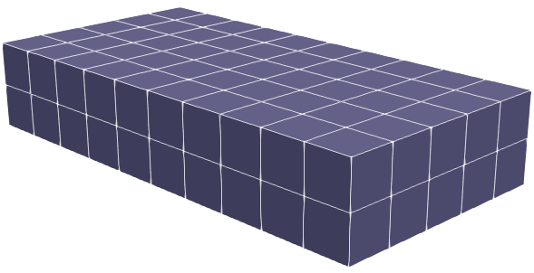
((a)) Homogenization

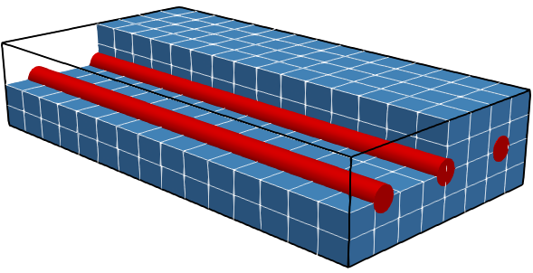
((b)) Embedded fibers in continuum

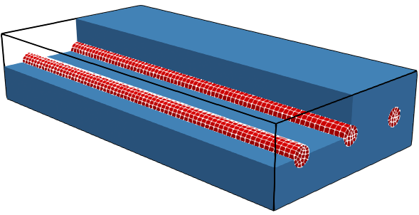
((c)) Fully resolved 3D model

Figure 1: Spectrum of modeling techniques for fibers embedded into three-dimensional solids [50]

On the one hand, homogenized formulations as depicted in Figure 1(a) incorporate all fiber information into the bulk constitutive law, usually leading to anisotropic formulations with preferential directions along the fiber orientation [3, 44]. On the other end of the spectrum, both bulk field and fibers are resolved as three-dimensional (3D) continua, cf. Figure 1(c), which allow to reuse existing constitutive models and finite element technology from classical 3D computational solid dynamics, enable the analysis of very detailed micro-mechanical features of individual fibers, and allow to incorporate advanced physical effects at the fiber-solid interface, yet come at significant computational cost. Finally, to unify the high model quality of fully resolved models with the efficiency of homogenized models, fibers can be represented by dimensionally reduced structural models such as beams or trusses, which are embedded at arbitrary positions into a 3D solid domain (cf. Figure 1(b)). In such mixed-dimensional 1D/3D models, the bulk field still portrays the same effects as in the fully resolved 3D model, but fibers are now reduced to a computationally efficient one-dimensional (1D) representation, making such models good candidates to study fiber-enhanced continua at large scale.

For the enforcement of coupling conditions in mixed-dimensional models, embedded mesh techniques are required. Although the imposition of constraints through Lagrange multipliers is well established in computational solid mechanics for both boundary-fitted meshes [41, 17] and embedded meshes [5, 21] as well as in computational contact mechanics [42, 43, 40, 57], the construction of stable Langrange multiplier spaces for mixed-dimensional beam-solid coupling still poses an open research question. Consequently, mixed-dimensional models for solid problems so far either use a penalty regularization to enforce the fiber-solid coupling constraints [14, 50, 52, 49, 24], employ a variationally consistent overlapping domain decomposition approach [25], or directly link embedded fibers to the surrounding volume discretization via the extended finite element method (XFEM) [27, 4]. Similarly, mixed-dimensional 1D/3D models are also available for other types of physics, e.g., in fluid/beam interaction (FBI) [20, 19, 28] to counteract 3D/3D fluid-solid interaction (FSI) models such as [32, 33].

Naturally, computational benefits of mixed-dimensional 1D/3D models are expected, since beam models require much fewer degrees of freedom (DOFs) than solid models to represent the embedded fibers. In [19], the mixed-dimensional approach reduces the number of DOFs for fiber modeling by 96% while keeping the L₂ error of the bulk field below 1.5%. Yet, the solution process of mixed-dimensional models at large scale is not widely studied in literature, but will be tackled in this contribution. In particular, when using Krylov methods to iteratively solve the arising linear systems, suitable preconditioners are required to sufficiently improve the spectral properties of the linear system [46]. Based on the framework of operator preconditioning [30], robust preconditioners have been proposed for 1D/3D domains coupled with Lagrange multipliers for applications in micro-circulation [12]. For penalty-based 1D/3D models and in particular for beam models serving as 1D models, preconditioners are yet to be developed.

In this paper, we will focus on our prior work on a regularized mortar-type embedding of geometrically exact nonlinear beams into 3D solids [50, 52] and will devise scalable preconditioners for the arising systems of linear equations. We will study key properties of the linear systems, in particular their loss of both diagonal dominance and block diagonal dominance due to the penalty contributions, and design a preconditioner that is mostly agnostic to these challenges. To this end, we will interpret the system matrix containing solid and beam contributions as a $2\times 2$ block matrix and employ approximate block factorizations to arrive at a Schur complement preconditioner. For the approximate inversion of the beam sub-block of the coupled system matrix, we will construct a sparse approximate inverse (SPAI) [18], which will not only allow to explicitly form an approximate Schur complement, but will also serve as a smoother within the Schur complement preconditioner. The original SPAI algorithm will be equipped with filtering and static enrichment algorithms to amplify its performance and robustness. To achieve scalability on parallel computing clusters, we will tackle the Schur complement equation itself with algebraic multigrid (AMG) methods from Trilinos/MueLu [6]. We will then study the computational performance and demonstrate weak scalability and applicability to practical use cases in a series of numerical experiments and investigate savings in wall clock time due to the reuse of the preconditioner throughout the entire load step. In sum, this contribution builds upon our prior work [50, 52] and provides these models with scalable iterative solvers to facilitate their efficient application to large models and systems with thousands of embedded fibers. Furthermore, this contribution constitutes the first presentation of a scalable, preconditioned iterative solver for truly 1D/3D models applied to beam-solid coupling with weak scalability demonstrated on a distributed memory cluster using the message passing interface (MPI) on up to 1000 MPI ranks.

The remainder of this manuscript is outlined as follows: Section 2 introduces the underlying mechanical problem of mixed-dimensional couplings of slender fibers embedded into solid continua and outlines the finite element discretization and the resulting linear systems. Relevant properties of these linear systems are then discussed in Section 3. The design of the preconditioner and its building blocks, in particular the SPAI algorithm, will be detailed in Section 4. In Section 5, we will study the numerical properties of individual components of the preconditioner and assess its performance and scalability when applied to academic and engineering test cases. Section 6 will summarize our findings and hint at future research directions.

2 Mixed-dimensional modeling of fiber/solid systems

Since this manuscript concerns itself with preconditioner development for the mixed-dimensional modeling of the interaction of solid continua with slender fibers, we only give a brief introduction into the governing equations, discretization and coupling approach presented in [50, 52]. For a broader overview of the fundamentals of beam-solid interaction, the interested reader is referred to [53].

2.1 Pure solid problem

The 3D solid bodies considered in this work are modeled as hyperelastic Boltzmann continua. The weak form of the equation of elastostatics describing the deformation of the solid body is given as

$$\delta W^{\mathcal{S}}=\int_{\Omega^{\mathcal{S}}}\bm{S}:\delta\bm{E}\;\mathrm{d}V-\int_{\Omega^{\mathcal{S}}}\bm{b}\cdot\delta\bm{u}^{\mathcal{S}}\;\mathrm{d}V-\int_{\Gamma^{\mathcal{S}}}\bm{t}\cdot\delta\bm{u}^{\mathcal{S}}\;\mathrm{d}A=0$$

with $\bm{u}^{\mathcal{S}}$ being the solid displacement field, $\bm{S}$ and $\bm{E}$ representing the second Piola–Kirchhoff stress tensor and the Green–Lagrange strain tensor, $\bm{b}$ denoting the body forces, $\bm{t}$ standing for the external traction field, and $\delta$ indicating virtual, but kinematically admissible quantities in line with the concept of virtual work. Furthermore, $\Omega^{\mathcal{S}}$ is the solid domain and $\Gamma^{\mathcal{S}}$ is the Neumann boundary of the solid domain. In this work, all quantities denoted with an $(\cdot)^{\mathcal{S}}$ are associated with the solid continuum. For the spatial discretization of the solid domain, we employ displacement-based isoparametric finite elements interpolated by Lagrange polynomials resulting in the following discretized linear system

$$\mathbf{K}_{ss}^{\mathcal{S}}\Delta\mathbf{d}^{\mathcal{S}}\\ =-\mathbf{f}_{s}^{\mathcal{S}}$$

to be solved in every iteration of the Newton solver. Therein, $\mathbf{f}_{s}^{\mathcal{S}}$ represents the nonlinear residual vector and $\mathbf{K}_{ss}^{\mathcal{S}}$ denotes its linearization, i.e., the solid stiffness matrix. The discrete displacement vector and its increment are given by $\mathbf{d}^{\mathcal{S}}$ and $\Delta\mathbf{d}^{\mathcal{S}}$, respectively.

2.2 Coupled beam-solid system with Simo–Reissner beam formulation

In the scope of this publication, Simo–Reissner (SR) and torsion-free Kirchhoff–Love (TF) beam theories are considered. With respect to the coupled beam-solid problem, the SR beam theory results in the most general coupling formulation. We first describe the coupled problem based on a SR beam formulation and defer the use of TF beam formulations to Section 2.3.

The general weak form for a 1D Cosserat continuum (applicable to SR and TF beam theory) is given by

$$\delta W^{\mathcal{B}}=\delta\Pi_{int,(\cdot)}^{\mathcal{B}}-\delta W_{ext}^{\mathcal{B}}=0,$$

where $\delta\Pi_{int,(\cdot)}^{\mathcal{B}}$ denotes the variation of the internal elastic energy function and $\delta W_{ext}^{\mathcal{B}}$ is the external virtual work acting on the beam. All quantities denoted with the superscript $(\cdot)^{\mathcal{B}}$ are associated with beam contributions. The internal elastic energy for a SR beam, i.e., a shear-deformable beam with six local modes of deformation, reads

$$\delta\Pi_{int,\mathrm{SR}}^{\mathcal{B}}=\frac{1}{2}\int_{\Omega^{\mathcal{B}}}\Gamma^{\mathrm{T}}\bm{C}_{F}\Gamma+\Omega^{\mathrm{T}}\bm{C}_{M}\Omega\;\mathrm{d}s.$$

Here, $\Gamma$ represents the material deformation, $\Omega$ the material curvature, and $\textbf{C}_{F}$ as well as $\textbf{C}_{M}$ are the respective constitutive matrices for the translational and rotational deformation modes. We refer the interested reader to [35, 36] for more details on the SR beam theory and its finite element discretization.

The weak form of the beam is defined on the undeformed 1D centerline domain $\Omega^{\mathcal{B}}$. The spatial interpolation of the beam finite elements is tailored to the particular beam model in order to ensure objectivity of the discrete formulation. The interpolation of the beam centerline position employs $C^{1}$-continuous third-order Hermite shape functions [36]. An objective interpolation of the finite cross section orientations is a non-trivial task and results in a highly nonlinear and deformation-dependent interpolation strategy. For a more detailed description of this topic, the reader is referred to [36] and the references therein. The resulting linearized system of a pure SR beam problem reads

$$\left(\begin{matrix}\mathbf{K}_{rr}^{\mathcal{B}}&\mathbf{K}_{r\theta}^{\mathcal{B}}\\ \mathbf{K}_{\theta r}^{\mathcal{B}}&\mathbf{K}_{\theta\theta}^{\mathcal{B}}\end{matrix}\right)\left(\begin{matrix}\Delta\mathbf{d}^{\mathcal{B}}\\ \Delta\bm{\theta}^{\mathcal{B}}\\ \end{matrix}\right)=-\left(\begin{matrix}\mathbf{f}_{r}^{\mathcal{B}}\\ \mathbf{f}_{\theta}^{\mathcal{B}}\end{matrix}\right).$$

To clarify the following equations and simplifications in the TF case, the global discrete beam centerline degrees of freedom $\mathbf{d}^{\mathcal{B}}$ are gathered together as are the global beam orientational degrees of freedom $\bm{\theta}^{\mathcal{B}}$. Therefore, the beam stiffness matrix is written as a $2\times 2$ block system with the individual blocks $\mathbf{K}_{ab}^{\mathcal{B}}$ with indices $a,b\in\{r,\theta\}$. Similarly, the residual is split into positional and rotational contributions $\mathbf{f}_{r}^{\mathcal{B}}$ and $\mathbf{f}_{\theta}^{\mathcal{B}}$, respectively.

To fully embed the beam in the solid matrix, the following six local coupling constraints are defined:

$$\bm{0} =\bm{r}^{\mathcal{B}}-\bm{x}^{\mathcal{S}}\ \text{on\ }\Omega^{\mathcal{B}},$$ (1)

$$\bm{0} =\bm{\psi}^{\mathcal{BS}}\ \text{on\ }\Omega^{\mathcal{B}}.$$ (2)

Here, $\bm{r}^{\mathcal{B}}$ is the beam centerline position vector, $\bm{x}^{\mathcal{S}}$ is the solid position vector, and $\bm{\psi}^{\mathcal{BS}}$ denotes the (pseudo-)rotation vector describing the relative rotation between a suitable orthonormal triad field in the solid domain and the beam cross section orientation. The constraints given in (1) are referred to as the positional coupling constraints, since they enforce the position of the beam cross section centroid to be coupled to the underlying solid. In a similar manner, (2) is referred to as rotational coupling since a vanishing relative rotation enforces the beam cross section orientation to be coupled to the solid domain. For a more elaborate discussion on the coupling constraints, the interested reader is referred to [50, 52]. The coupling constraints (1) and (2) are enforced via a Lagrange multiplier method. The total Lagrange multiplier potential reads

$$\Pi_{\lambda,\mathrm{SR}}=\int_{\Omega^{\mathcal{B}}}({\bm{\lambda}}^{\mathcal{V}})^{\mathrm{T}}(\bm{r}^{\mathcal{B}}-\bm{x}^{\mathcal{S}})\;\mathrm{d}s+\int_{\Omega^{\mathcal{B}}}({\bm{\lambda}}^{\mathcal{R}})^{\mathrm{T}}\bm{\psi}\;\mathrm{d}s,$$ (3)

where ${\bm{\lambda}}^{\mathcal{V}}$ and ${\bm{\lambda}}^{\mathcal{R}}$ are the Lagrange multiplier fields introduced to enforce the positional and rotational coupling, respectively. Accordingly, quantities denoted with ${(\cdot)}^{\mathcal{V}}$ and ${(\cdot)}^{\mathcal{R}}$ refer to positional and rotational coupling, respectively.

For the spatial interpolation of the Lagrange multiplier fields, we resort to the mortar-type approach and software implementation of [50, 52]. There it is shown that a linear interpolation of the Lagrange multiplier field with a subsequent penalty regularization of the saddle point system results in a stable coupling formulation for our envisioned application range. The resulting global discrete Lagrange multiplier vectors for positional and rotational coupling are denoted with ${\bm{\uplambda}}^{\mathcal{V}}$ and ${\bm{\uplambda}}^{\mathcal{R}}$, respectively. Variation of the coupling potential (3) and insertion of the spatially discretized quantities results in the weak form of the coupling formulation. With that we can now state the global discretized residual vector for the coupled problem:

$$\left(\begin{matrix}\mathbf{f}_{r}^{\mathcal{B}}+{\mathbf{f}}^{\mathcal{V}}_{mt,r}\\ \mathbf{f}_{\theta}^{\mathcal{B}}+{\mathbf{f}}^{\mathcal{R}}_{mt,\theta}\\ \mathbf{f}^{\mathcal{S}}_{s}+{\mathbf{f}}^{\mathcal{V}}_{mt,s}+{\mathbf{f}}^{\mathcal{R}}_{mt,s}\\ {\mathbf{g}}^{\mathcal{V}}\\ {\mathbf{g}}^{\mathcal{R}}\\ \end{matrix}\right)=\mathbf{0}.$$

Here, ${\mathbf{g}}^{\mathcal{V}}$ and ${\mathbf{g}}^{\mathcal{R}}$ are the constraint residual vectors for positional and rotational coupling, respectively. Moreover, ${\mathbf{f}}_{mt,(\cdot)}^{(\cdot)}$ are the discrete coupling force contributions required to enforce the action of the Lagrange multipliers on the beam and solid degrees of freedom. We resort to a penalty regularization with the penalty parameters ${\epsilon}^{\mathcal{V}}>0$ and ${\epsilon}^{\mathcal{R}}>0$ to express the Lagrange multiplier unknowns ${\bm{\uplambda}}^{\mathcal{V}}$ and ${\bm{\uplambda}}^{\mathcal{R}}$ in terms of beam and solid unknowns, i.e.,

$${\bm{\uplambda}}^{\mathcal{V}} \approx{\epsilon}^{\mathcal{V}}({\mathbf{V}}^{\mathcal{V}})^{-1}{\mathbf{g}}^{\mathcal{V}},$$ (4)

$${\bm{\uplambda}}^{\mathcal{R}} \approx{\epsilon}^{\mathcal{R}}({\mathbf{V}}^{\mathcal{R}})^{-1}{\mathbf{g}}^{\mathcal{R}}.$$ (5)

Therein, the diagonal matrices ${\mathbf{V}}^{\mathcal{V}}$ and ${\mathbf{V}}^{\mathcal{R}}$ are scaling matrices to scale the regularized equations in order to pass patch-test like problems, cf. [50]. With the penalty regularization, the Lagrange multipliers are no longer unknowns. Thus, we can state the final linearized system to be solved in every Newton iteration:

$$\begin{split}&\left(\begin{matrix}\mathbf{K}_{rr}^{\mathcal{B}}+{\epsilon}^{\mathcal{V}}\mathbf{D}^{\mathrm{T}}({\mathbf{V}}^{\mathcal{V}})^{-1}\mathbf{D}&\mathbf{K}_{r\theta}^{\mathcal{B}}&-{\epsilon}^{\mathcal{V}}\mathbf{D}^{\mathrm{T}}({\mathbf{V}}^{\mathcal{V}})^{-1}\mathbf{M}\\ \mathbf{K}_{\theta r}^{\mathcal{B}}&\mathbf{K}_{\theta\theta}^{\mathcal{B}}+\mathbf{Q}_{\theta\theta}+{\epsilon}^{\mathcal{R}}\mathbf{Q}_{\theta\lambda}({\mathbf{V}}^{\mathcal{R}})^{-1}\mathbf{Q}_{\lambda\theta}&\mathbf{Q}_{\theta s}+{\epsilon}^{\mathcal{R}}\mathbf{Q}_{\theta\lambda}\mathbf{V}^{-1}\mathbf{Q}_{\lambda s}\\ -{\epsilon}^{\mathcal{V}}\mathbf{M}^{\mathrm{T}}({\mathbf{V}}^{\mathcal{V}})^{-1}\mathbf{D}&\mathbf{Q}_{s\theta}+{\epsilon}^{\mathcal{R}}\mathbf{Q}_{s\lambda}({\mathbf{V}}^{\mathcal{R}})^{-1}\mathbf{Q}_{\lambda\theta}&\mathbf{K}_{ss}^{\mathcal{S}}+\mathbf{Q}_{ss}+{\epsilon}^{\mathcal{V}}\mathbf{M}^{\mathrm{T}}({\mathbf{V}}^{\mathcal{V}})^{-1}\mathbf{M}+{\epsilon}^{\mathcal{R}}\mathbf{Q}_{s\lambda}({\mathbf{V}}^{\mathcal{R}})^{-1}\mathbf{Q}_{\lambda s}\\ \end{matrix}\right)\left(\begin{matrix}\Delta\mathbf{d}^{\mathcal{B}}\\ \Delta\bm{\theta}^{\mathcal{B}}\\ \Delta\mathbf{d}^{\mathcal{S}}\\ \end{matrix}\right)\\ &=-\left(\begin{matrix}\mathbf{f}_{r}^{\mathcal{B}}\\ \mathbf{f}_{\theta}^{\mathcal{B}}\\ \mathbf{f}_{s}^{\mathcal{S}}\\ \end{matrix}\right)\end{split}.$$ (6)

Here, $\mathbf{D}$ and $\mathbf{M}$ are the so called mortar matrices for positional coupling, which only depend on the reference configuration, i.e., they are constant. The matrices $\mathbf{Q}_{ab}$ with $a,b\in\{s,\theta,\lambda\}$ are the coupling matrices for rotational coupling, which depend on the current configuration. We refer to the original publications [50, 52] for details of the linearization procedure.

2.3 Coupled beam-solid system with torsion-free (TF) beam formulation

The torsion-free Kirchhoff–Love (TF) beam formulation (see [35, 36]) represents a special case of the Simo–Reissner beam theory, where the assumptions of vanishing shear and torsion deformations are incorporated in the beam model and the resulting finite element formulation can be described solely by displacement degrees of freedom. The assumptions are valid for fibers with high slenderness ratios, a double symmetric cross section and a straight centerline in the reference configuration. For such fibers, the TF beam formulation results in an even more efficient numerical model than the SR formulation presented in the previous section. The internal energy of a TF beam reads

$$\delta\Pi_{int,\mathrm{TF}}^{\mathcal{B}}=\frac{1}{2}\int_{\Omega^{\mathcal{B}}}EA\varepsilon^{2}+EI\kappa^{2}\;\mathrm{d}s$$

with $E$ denoting the Young’s modulus, $A$ the cross section area, $I$ the moment of inertia, $\varepsilon$ the axial tension and $\kappa$ the scalar curvature, respectively. The TF beam formulation requires a $C^{1}$-continuous centerline interpolation of centerline positions $\bm{r}$, which is realized with third-order Hermite polynomials [35].

As the only field of unknowns along the TF beam centerline is a translation field, the total Lagrange multiplier potential of the coupling constraints in (3) simplifies to

$$\Pi_{\lambda,\mathrm{TF}}=\int_{\Gamma}({\bm{\lambda}}^{\mathcal{V}})^{\mathrm{T}}(\bm{r}^{\mathcal{B}}-\bm{x}^{\mathcal{S}})\;\mathrm{d}s$$

i.e., there is no rotational coupling for TF beams. The same penalty regularization as stated in (4) is employed, resulting in the following global linearized system :

$$\left(\begin{matrix}\mathbf{K}_{rr}^{\mathcal{B}}+{\epsilon}^{\mathcal{V}}\mathbf{D}^{\mathrm{T}}({\mathbf{V}}^{\mathcal{V}})^{-1}\mathbf{D}&-{\epsilon}^{\mathcal{V}}\mathbf{D}^{\mathrm{T}}({\mathbf{V}}^{\mathcal{V}})^{-1}\mathbf{M}\\ -{\epsilon}^{\mathcal{V}}\mathbf{M}^{\mathrm{T}}({\mathbf{V}}^{\mathcal{V}})^{-1}\mathbf{D}&\mathbf{K}_{ss}^{\mathcal{S}}+{\epsilon}^{\mathcal{V}}\mathbf{M}^{\mathrm{T}}({\mathbf{V}}^{\mathcal{V}})^{-1}\mathbf{M}\end{matrix}\right)\left(\begin{matrix}\Delta\mathbf{d}^{\mathcal{B}}\\ \Delta\mathbf{d}^{\mathcal{S}}\\ \end{matrix}\right)=-\left(\begin{matrix}\mathbf{f}_{r}^{\mathcal{B}}\\ \mathbf{f}_{s}^{\mathcal{S}}\\ \end{matrix}\right).$$ (7)

Again, for a more detailed information on the derivations, the interested reader is referred to [50]. It should be noted, that the coupling contributions in (7), i.e., $\mathbf{D}$ and $\mathbf{M}$, are constant due to the coupling taking place in the reference configuration.

3 Characteristics of linear systems arising in beam-solid coupling

To be able to construct efficient algebraic block preconditioning techniques to accelerate the convergence of the outer Krylov solver, certain matrix properties of the underlying linear systems specified in (LABEL:eq:RotationCouplingLinearSystem) and (7) are of particular interest. A short explanation regarding conditioning, block diagonal dominance, symmetry and sparsity pattern is given below. For the sake of simplicity, the block systems in (LABEL:eq:RotationCouplingLinearSystem) and (7) are both abbreviated with the compact notation

$$\left(\begin{matrix}\mathbf{A}&\mathbf{B}_{1}^{\mathrm{T}}\\ \mathbf{B}_{2}&\mathbf{C}\\ \end{matrix}\right)\left(\begin{matrix}\mathbf{x}^{\mathcal{B}}\\ \mathbf{x}^{\mathcal{S}}\\ \end{matrix}\right)=\left(\begin{matrix}\mathbf{b}^{\mathcal{B}}\\ \mathbf{b}^{\mathcal{S}}\\ \end{matrix}\right)\quad\text{ with }\mathbf{r}=\left(\begin{matrix}\mathbf{r}^{\mathcal{B}}\\ \mathbf{r}^{\mathcal{S}}\\ \end{matrix}\right)=\left(\begin{matrix}\mathbf{b}^{\mathcal{B}}\\ \mathbf{b}^{\mathcal{S}}\\ \end{matrix}\right)-\left(\begin{matrix}\mathbf{A}&\mathbf{B}_{1}^{\mathrm{T}}\\ \mathbf{B}_{2}&\mathbf{C}\\ \end{matrix}\right)\left(\begin{matrix}\mathbf{x}^{\mathcal{B}}\\ \mathbf{x}^{\mathcal{S}}\\ \end{matrix}\right)$$ (8)

throughout the remainder of the publication, where we have grouped the unknowns based on their physical meaning, i.e., being associated with the beams or the background solid. The concrete identification of individual matrix blocks in (8) with the linear systems from Sections 2.2 and 2.3 depends on the employed beam theory. In the case of a SR beam theory, the individual blocks are defined such that (8) represents (LABEL:eq:RotationCouplingLinearSystem) with $\mathbf{b}^{\mathcal{B}}=(\Delta(\mathbf{d}^{\mathcal{B}})^{\mathrm{T}},(\Delta\bm{\theta}^{\mathcal{B}})^{\mathrm{T}})^{\mathrm{T}}$ and $\mathbf{b}^{\mathcal{S}}=\Delta\mathbf{d}^{\mathcal{S}}$. For the TF case, (8) represents (7) with $\mathbf{b}^{\mathcal{B}}=\Delta\mathbf{d}^{\mathcal{B}}$ and $\mathbf{b}^{\mathcal{S}}=\Delta\mathbf{d}^{\mathcal{S}}$. Generally speaking, $\mathbf{A}$ denotes the matrix block containing the beam stiffness matrices $\mathbf{K}_{ab}^{\mathcal{B}}$ as well as stiffness and penalty contributions of the coupling constraints. In similar fashion, the sub-block $\mathbf{C}$ refers to the sum of the solid stiffness matrix $\mathbf{K}_{ab}^{\mathcal{S}}$ and the respective interaction terms. The off-diagonal sub-blocks $\mathbf{B}_{1}^{\mathrm{T}}$ and $\mathbf{B}_{2}$ represent the remaining coupling terms between both fields, respectively.

3.1 Ill-conditioning due to penalty regularization

Due to the discretization and coupling approach introduced in Section 2, the linear system of equations suffers from ill-conditioning, which directly originates from the penalty parameters ${\epsilon}^{\mathcal{V}}$ and ${\epsilon}^{\mathcal{R}}$, that are steering the strength of the interaction between solid and fibers. Naturally, larger values of ${\epsilon}^{\mathcal{V}}$ and ${\epsilon}^{\mathcal{R}}$ lead to a more accurate constraint enforcement, however enlarge the eigenvalue spectrum of the matrix and, thus, worsen the conditioning problems.

3.2 Loss of block diagonal dominance

Independent of the actual choice of the beam model within beam-solid interaction, the matrices in the arising linear systems in (LABEL:eq:RotationCouplingLinearSystem) and (7) exhibit a 2 $\times$ 2 block structure based on a physically motivated grouping of unknowns into beam unknowns $\mathbf{x}^{\mathcal{B}}$ and solid unknowns $\mathbf{x}^{\mathcal{S}}$, respectively. This becomes particularly evident in the unified notation of (8). For a closer look at the arising matrices, we adopt the concept of block diagonal dominance for block matrices from [16]:

Definition 3.1 (Block diagonal dominance).

Let $\mathbf{H}\in\mathbb{C}^{N_{\mathrm{R}}\times N_{\mathrm{R}}}$ be a square block matrix with $N_{\mathrm{R}}$ block rows and block columns, respectively. With a given matrix norm $\left\|\left(\bullet\right)\right\|$, we assume $\mathbf{H}$ to only contain nonsingular matrix blocks $\mathbf{H}_{\iota\iota}$ on its main diagonal, i.e., $\det{\mathbf{H}_{\iota\iota}}\neq 0\,\forall\iota\in 1,\ldots,N_{\mathrm{R}}$. Then, a matrix $\mathbf{H}$ is referred to as block diagonally dominant, if

$$\sum_{\begin{subarray}{c}\zeta=1\\ \zeta\neq\iota\end{subarray}}^{N_{\mathrm{R}}}\left\|\mathbf{H_{\iota\zeta}}\right\|\leq\left\|\mathbf{H}_{\iota\iota}^{-1}\right\|^{-1}\quad\text{ for }\iota=1,\dots,N_{\mathrm{R}}.$$ (9)

In general, the matrices in (LABEL:eq:RotationCouplingLinearSystem) and (7) do not satisfy the conditions for block diagonal dominance as outlined in Definition 3.1. For illustration purposes, we consider the mixed-dimensional modeling approach from Section 2 in the practical case of fiber-reinforced solids, where the stiffness of the fibers is much higher than the stiffness of the embedding solid, i.e., $E^{\mathcal{B}}\gg E^{\mathcal{S}}$. To this end, we assume a fixed geometry and mesh, constant material parameters, and fiber and solid constitutive properties satisfying $E^{\mathcal{B}}\gg E^{\mathcal{S}}$. Since the projection operators $\mathbf{D}$ and $\mathbf{M}$ solely depend on the mesh, the only variable parameters left are ${\epsilon}^{\mathcal{V}}\gg 0$ and ${\epsilon}^{\mathcal{R}}\gg 0$. With increasing penalty parameters ${\epsilon}^{\mathcal{V}}$ and ${\epsilon}^{\mathcal{R}}$, the norm of the off-diagonal matrix blocks increases, too. In addition, the inversion of the diagonal matrix blocks results in denser matrices with a rapid growth of the norm and, thus, decreasing values on the right-hand side of inequality (9). For positional coupling, the block diagonal dominance property of the matrix becomes harder to achieve with an increasing penalty parameter ${\epsilon}^{\mathcal{V}}$, especially for ${\epsilon}^{\mathcal{V}}\approx E^{\mathcal{B}}$ as recommended for practical computations. The same holds true for the rotational coupling contributions for the recommended choice ${\epsilon}^{\mathcal{R}}\approx E^{\mathcal{B}}R^{2}$ with $R$ being the radius of the beam along the centerline (see [49]). To support this argumentation, we assess the property of block diagonal dominance for the first block row in (8), i.e., specifically the contribution of $\mathbf{A}$, by anticipating a small numerical example, in particular Test Case I introduced later in Section 5.1. Therein, the off-diagonal matrix block $\mathbf{B}_{1}$ exhibits a norm $\left\|\mathbf{B}_{1}\right\|=1.0153$, while the main diagonal block $\mathbf{A}$’s contribution evaluates to $\left\|\mathbf{A}^{-1}\right\|^{-1}=3.9202\cdot 10^{-8}$, hence violating the condition outlined in (9).

Due to this lack of block diagonal dominance, conventional block preconditioning methods based on block Jacobi or block Gauß–Seidel schemes are not applicable without major convergence problems (or even divergence) as already evidenced in [8, 11]. Independently, the individual matrix blocks on the main diagonal loose their diagonal dominance as well due to the penalty contributions. Hence, conventional relaxation-based smoothers can not be applied on individual blocks either.

3.3 Potential loss of symmetry

The symmetry of $\mathbf{A}$ is governed by the beam formulation at hand: TF beam models always result in a symmetric $\mathbf{A}$, while all other beam models yield a non-symmetric beam sub-block $\mathbf{A}$. For pure positional coupling as applied for TF beam models, the off-diagonal matrix block are symmetric, i.e., $\mathbf{B}_{1}=\mathbf{B}_{2}$. In contrast, the additional coupling of rotational degrees of freedom for SR beams introduces non-symmetric off-diagonal terms.

3.4 Sparsity pattern

Of special interest is the matrix graph $\mathcal{J}\left(\mathbf{A}\right)$ of the sub-block $\mathbf{A}$ related to the beam problem. Since we restrict ourselves so far to cases, where the embedded fibers do not interact with each other, but only with the surrounding solid, the matrix $\mathbf{A}$ features a block diagonal sparsity structure, where the size of the small blocks depends on the number of beam finite elements used to discretize each individual fiber. We will illustrate and study the sparsity pattern $\mathcal{J}\left(\mathbf{A}\right)$ for different test cases in Section 5.1, in particular in Figure 4.

4 Physics-based block preconditioning for beam-solid interaction

The construction of a preconditioner, that captures the coupling interactions properly and is tailored to the specific matrix properties, is crucial for an efficient and scalable solution process. Preconditioners based on approximate block factorizations have shown to be suited for similar problem types such as contact problems [57], incompressible flow [37, 15], FSI [26, 23], or magneto-hydro dynamics [8, 38, 39].

4.1 Schur complement based block factorization

Due to the lack of block diagonal dominance as discussed in Section 3 and the ill-conditioning of the matrix, we resort to a block factorization preconditioner based on a Schur complement. Specifically, we perform an approximate block factorization based on a SIMPLE-type approach [37]. To this end, the preconditioning matrix $\mathbf{P}$ can be written as

$$\mathbf{P}:=\left(\begin{matrix}\mathbf{A}&0\\ \mathbf{B}_{2}&\widehat{\mathbf{S}}\\ \end{matrix}\right)\left(\begin{matrix}\mathbf{I}&\widehat{\mathbf{A}}^{-1}\mathbf{B}_{1}^{\mathrm{T}}\\ 0&\frac{1}{\alpha}\mathbf{I}\\ \end{matrix}\right)=\left(\begin{matrix}\mathbf{A}&\mathbf{A}\widehat{\mathbf{A}}^{-1}\mathbf{B}_{1}^{\mathrm{T}}\\ \mathbf{B}_{2}&\frac{1}{\alpha}\mathbf{C}+\left(1-\frac{1}{\alpha}\right)\mathbf{B}_{2}\widehat{\mathbf{A}}^{-1}\mathbf{B}_{1}^{\mathrm{T}}\\ \end{matrix}\right)\approx\left(\begin{matrix}\mathbf{A}&\mathbf{B}_{1}^{\mathrm{T}}\\ \mathbf{B}_{2}&\mathbf{C}\\ \end{matrix}\right)$$

with $\widehat{\mathbf{A}}$ and $\widehat{\mathbf{S}}$ denoting easy-to-invert approximations of the sub-matrix $\mathbf{A}$ from (8) and the Schur complement $\mathbf{S}:=\mathbf{C}+\mathbf{B}_{2}\mathbf{A}^{-1}\mathbf{B}_{1}^{\mathrm{T}}$, respectively, and $\alpha>0$ being a relaxation factor. Expressing the application of the preconditioner as a fixed-point iteration over the index $k$, one application of the preconditioner yields

$$\left(\begin{matrix}\mathbf{x}^{\mathcal{B},k+1}\\ \mathbf{x}^{\mathcal{S},k+1}\\ \end{matrix}\right)=\left(\begin{matrix}\mathbf{x}^{\mathcal{B},k}\\ \mathbf{x}^{\mathcal{S},k}\\ \end{matrix}\right)+\left(\begin{matrix}\mathbf{A}&\mathbf{A}\widehat{\mathbf{A}}^{-1}\mathbf{B}_{1}^{\mathrm{T}}\\ \mathbf{B}_{2}&\frac{1}{\alpha}\mathbf{C}+\left(1-\frac{1}{\alpha}\right)\mathbf{B}_{2}\widehat{\mathbf{A}}^{-1}\mathbf{B}_{1}^{\mathrm{T}}\\ \end{matrix}\right)^{-1}\left[\left(\begin{matrix}\mathbf{b}^{\mathcal{B}}\\ \mathbf{b}^{\mathcal{S}}\\ \end{matrix}\right)-\left(\begin{matrix}\mathbf{A}&\mathbf{B}_{1}^{\mathrm{T}}\\ \mathbf{B}_{2}&\mathbf{C}\\ \end{matrix}\right)\left(\begin{matrix}\mathbf{x}^{\mathcal{B},k}\\ \mathbf{x}^{\mathcal{S},k}\\ \end{matrix}\right)\right],$$

which is usually tackled via a a predictor-corrector scheme by first solving an equation related to the beam contribution and afterwards a second one related to the Schur complement.

Both quality and computational cost of the preconditioner are mainly governed by the choice $\widehat{\mathbf{A}}$ and $\widehat{\mathbf{S}}$ to approximate $\mathbf{A}$ and $\mathbf{S}$, respectively. In traditional Schur complement based block preconditioners, the inverse $\widehat{\mathbf{A}}^{-1}\approx\mathbf{A}^{-1}$ appearing due to the block factorization and also in the Schur complement calculation itself is often approximated by some diagonal matrix, since the inversion of a diagonal matrix comes at a negligible computational cost. The most simple approach is to base the inverse approximation on the diagonal part of the $M\times M$ matrix $\mathbf{A}$ resulting in $\widehat{\mathbf{A}}=\mathrm{diag}\left(a_{ii}\right),i=1,\ldots,M$. Another well-known method referred to as SIMPLEC takes the row sums of $\mathbf{A}$ [55], reading

$$\widehat{\mathbf{A}}=\mathrm{diag}\left(\sum_{j=1}^{M}\left|a_{ij}\right|\right),\quad i=1,\ldots,M.$$

However, such simple diagonal approximations cannot be used in the present scenario since $\mathbf{A}$ lacks diagonal dominance, cf. Section 3.2. Since $\mathbf{A}$ resembles the sub-block related to the beam equations, which themselves yield a block diagonal structure of $\mathbf{A}$, a more sophisticated explicit approximation scheme of the inverse can be applied taking this particular sparsity structure into account (see Section 4.2).

To this end, the choice of $\widehat{\mathbf{S}}$ is governed by $\widehat{\mathbf{A}}$ and the relaxation parameter $\alpha$.

4.2 Explicit sparse inverse approximation

Although in general the inverse of the sparse matrix $\mathbf{A}$ cannot be expected to be sparse as well, explicit sparse approximate inverses aim to create an explicit matrix representation ${\mathbf{A}}^{\ast}$ of the approximation of the exact inverse $\mathbf{A}^{-1}$, that itself is still a sparse matrix. Ideally, $\mathrm{nnz}\left({\mathbf{A}}^{\ast}\right)$, the number of non-zeros of ${\mathbf{A}}^{\ast}$, does not exceed $\mathrm{nnz}\left(\mathbf{A}\right)$, since a matrix-vector product with ${\mathbf{A}}^{\ast}$ must be performed at each Krylov iteration [18]. Although incomplete LU factorizations fall into that category, they require considerable effort to parallelize [10].

To take advantage of the block diagonal structure of $\mathbf{A}$, we pursue a fully parallelizable approach to construct an explicit sparse approximate inverse ${\mathbf{A}}^{\ast}$ of the matrix $\mathbf{A}$ based on the minimization of the Frobenius norm of the residual matrix $\mathbf{A}{\mathbf{A}}^{\ast}-\mathbf{I}$, see [18, 48]. By choosing an appropriate sparsity pattern $\mathcal{J}\left({\mathbf{A}}^{\ast}\right)$ for the sparse approximate inverse ${\mathbf{A}}^{\ast}$ from the set $\mathcal{J}$ describing all known patterns, the following least-squares problem needs to be solved:

$$\min_{\mathcal{J}\left({\mathbf{A}}^{\ast}\right)\;\in\;\mathcal{J}}\left\|\mathbf{A}{\mathbf{A}}^{\ast}-\mathbf{I}\right\|_{\mathrm{F}}.$$ (10)

We represent the minimization procedure to compute ${\mathbf{A}}^{\ast}$ by the operation ${\mathbf{A}}^{\ast}\leftarrow\mathcal{M}\left(\mathbf{A},\mathcal{J}\left({\mathbf{A}}^{\ast}\right)\right)$. To this end, (10) requires to select an appropriate sparsity pattern $\mathcal{J}\left({\mathbf{A}}^{\ast}\right)$ and a practical approach to the minimization of the Frobenius norm in a distributed memory environment, which we will address in Sections 4.2.1 and 4.2.2, respectively.

4.2.1 Selection of a sparsity pattern for the sparse approximate inverse calculation

The main challenge in (10) is the selection of a sparsity pattern $\mathcal{J}\left({\mathbf{A}}^{\ast}\right)$ to be used as input into the minimization procedure. An appropriate pattern needs to contain enough information of the inverse by retaining high values, but should also act as a filter to remove small entries in order to reduce fill-in. Straightforward approaches are based on a static sparsity pattern selection and include the choices $\mathcal{J}\left({\mathbf{A}}^{\ast}\right):=\mathcal{J}\left(\mathbf{A}\right)$ and $\mathcal{J}\left({\mathbf{A}}^{\ast}\right):=\mathcal{J}\left(\mathbf{A}^{\mathrm{T}}\right)$, which are easy to obtain, but do not guarantee a good approximation quality. Especially in cases with a partially known sparsity structure of the inverse, e.g., for block-diagonal matrices such as $\mathbf{A}$ in (8), more advanced static selections are able to deliver a satisfying approximation, yet not requiring dynamic pattern selection approaches as proposed in [18].

In this work, we follow the static pattern selection proposed in [9] and use powers of a sparsified version $\underline{\mathcal{J}\left(\mathbf{A}\right)}$ of the graph $\mathcal{J}\left(\mathbf{A}\right)$ of the original matrix $\mathbf{A}$ to obtain an enriched sparsity pattern to be used for the minimization in (10). First, $\underline{\mathcal{J}\left(\mathbf{A}\right)}$ is obtained through a thresholding of $\mathcal{J}\left(\mathbf{A}\right)$ based on the entries in $\mathbf{A}$ and using a drop-off tolerance $\sigma$. We represent this thresholding by the filter operation

$$\underline{\mathcal{J}\left(\mathbf{A}\right)}\leftarrow\mathcal{F}_{\mathcal{J}}\left({\mathbf{A}},\sigma\right)$$

delivering individual entries $\underline{j\left(\mathbf{A}\right)_{ij}}$ of the filtered graph via

$$\underline{j\left(\mathbf{A}\right)_{ij}}:=\begin{cases}1\quad\text{if}\;i=j\;\text{or}\;\left|d_{i}^{-\frac{1}{2}}a_{ij}d_{i}^{-\frac{1}{2}}\right|>\sigma,\\ 0\quad\text{otherwise},\end{cases}\quad\text{where}\quad d_{i}:=\begin{cases}\left|a_{ii}\right|\quad\text{if}\;\left|a_{ii}\right|>0,\\ 1\quad\text{otherwise}.\end{cases}$$ (11)

The additional Jacobi scaling in (11) simplifies the thresholding and choosing of $\sigma$ if $\mathbf{A}$ is poorly scaled. In a second step, a refined sparsity pattern $\mathcal{J}\left(\mathbf{A}^{\ell}\right)$ is calculated by taking powers $\ell$ of the sparsified graph $\underline{\mathcal{J}\left(\mathbf{A}\right)}$, reading

$$\mathcal{J}\left({\mathbf{A}}^{\ast}\right)\leftarrow\mathcal{R}\left(\underline{\mathcal{J}\left(\mathbf{A}\right)},\ell\right).$$

The matrix $\mathbf{A}^{\ell}$ is never calculated explicitly, but the powers are directly computed on its sparsified graph $\underline{\mathcal{J}\left(\mathbf{A}\right)}$.

4.2.2 Evaluation of the Frobenius norm on a parallel computer

Due to the 2-norm compatibility of the Frobenius norm, the problem can be decoupled into a sum of Euclidian norms, reading

$$\min_{\mathcal{J}\left({\mathbf{A}}^{\ast}\right)\;\in\;\mathcal{J}}\left\|\mathbf{A}{\mathbf{A}}^{\ast}-\mathbf{I}\right\|_{\mathrm{F}}=\sum_{i=1}^{M}\min_{\mathcal{J}\left({\mathbf{A}}^{\ast}\right)\;\in\;\mathcal{J}}\left\|\left(\mathbf{A}{\mathbf{A}}^{\ast}-\mathbf{I}\right)\mathbf{e}_{i}\right\|_{2}^{2}=\sum_{i=1}^{M}\min_{\mathcal{J}\left({\mathbf{A}}^{\ast}_{i}\right)\;\in\;\mathcal{J}_{i}}\left\|\mathbf{A}{\mathbf{A}}^{\ast}_{i}-\mathbf{e}_{i}\right\|_{2}^{2},$$

which can be solved independently for each row $i=1,\ldots,M$ of ${\mathbf{A}}^{\ast}$. Since the matrix $\mathbf{A}$ is usually stored in a row-wise distribution, where each parallel process stores a subset of all rows of $\mathbf{A}$, this decomposition renders the method, besides an initial communication step, inherently parallel. To this end, calculating a row of the approximate inverse means solving a small least-squares problem by applying a dense QR factorization.

4.2.3 Practical algorithm

In practice, one usually does not solve (10) directly, but rather combines it with some pre- and post-operations, foremost the graph computation from Section 4.2.1 and the handling of the Frobenius norm outlined in Section 4.2.2. In addition, it appears beneficial to perform a post-filtering of ${\mathbf{A}}^{\ast}$ by dropping all entries with $\left|{a}^{\ast}_{ij}\right|<\sigma\quad\forall i,j=1,\ldots,M$ to further reduce fill-in of $\widehat{\mathbf{A}}^{-1}$ and, thus, the cost of applying the preconditioner [9]. The post-filtering will be denoted by the operator $\mathcal{F}_{\mathbf{A}}\left({\mathbf{A}}^{\ast},\sigma\right)$.

We summarize all the steps to compute the sparse approximate inverse ${\mathbf{A}}^{\ast}$ in Figure 2.

Figure 2: Optional (gray) and mandatory (orange) steps of the SPAI computation and its flow of information with computed data (in boxes) and user parameters (in circles)

Therein, optional steps are marked in gray, while the mandatory computation of ${\mathbf{A}}^{\ast}$ is highlighted in orange. User-given data to configure the individual steps is depicted in circles, while computed input and output data is put into rectangular boxes. The arrows indicate the flow of data between the individual steps.

Even tough the method can be steered quite effectively by the refinement level $\ell$ and threshold tolerance $\sigma$, there are still several problems to avoid. The method can still produce rather dense matrices with poor approximation quality. Depending on the threshold parameter $\sigma$, an aggressive dropping of values might result in a loss of information, which again results in a poor result and the approximation of the inverse might even be singular.

4.3 One-level approach for the predictor step

The first linear equation to be solved inside the block preconditioner resembling the predictor step consists of the beam equation with matrix $\mathbf{A}$:

$$\mathbf{A}\mathbf{x}^{\mathcal{B},k+\frac{1}{2}}=\mathbf{b}^{\mathcal{B},k}-\mathbf{B}_{1}^{\mathrm{T}}\mathbf{x}^{\mathcal{S},k}.$$ (12)

Following the assumptions made in Section 3.2, traditional smoothing approaches are not applicable to the linear system without a major loss in convergence properties.

Based on the explicit sparse approximate inverse calculation for the approximation of the Schur complement, a rather good approximation $\widehat{\mathbf{A}}^{-1}$ is already available. Following [7], the sparse approximate inverse is reused as smoother by applying the following fixed-point iteration over index $m$ to (12):

$$\mathbf{x}^{\mathcal{B},k+\frac{1}{2},m+1}=\mathbf{x}^{\mathcal{B},k+\frac{1}{2},m}-\widehat{\mathbf{A}}^{-1}\left(\mathbf{b}^{\mathcal{B},k,m}-\mathbf{B}_{1}^{\mathrm{T}}\mathbf{x}^{\mathcal{S},k,m}\right).$$ (13)

A comparison to more traditional smoothers, e.g., Jacobi and Gauß–Seidel methods, can also be found in the original publication [7].

Remark 4.1 (Challenges for multilevel methods).

Expanding the solution procedure of the predictor step to an AMG approach to solve the beam related equation is challenging, as there are still several open questions around the construction of AMG hierarchies for beam models: the beams are represented as 1D elements, for which a suitable coarsening scheme to form aggregates for coarser multigrid (MG) levels is still part of active research. Even with appropriate coarsening, fibers discretized with only a few elements would quickly form single-node aggregates being suboptimal for the restrictor and prolongator construction as well as effectively stalling the coarsening process. The addition of rotational components into the beam equation introduces another difficulty, as nodes with a different number of DOFs exist, hindering the application of conventional aggregation strategies. To project and, thus, treat important error modes correctly on coarser levels, a proper near nullspace has to be constructed, which highly depends on the underlying beam formulation. For the use cases presented in this publication, which mostly feature a small number of beam elements used to discretize a fiber, the SPAI smoother from (13) proved to be very competitive in terms of approximation quality of the inverse, computational efficiency and weak scaling behavior, see Section 5.

4.4 Multilevel approach for the correction step

The computationally most demanding part of the preconditioning algorithm involves the solution procedure for the Schur complement equation given as

$$\widehat{\mathbf{S}}\mathbf{x}^{\mathcal{S},k+\frac{1}{2}}=\mathbf{b}^{\mathcal{S},k}-\mathbf{C}\mathbf{x}^{\mathcal{S},k}-\mathbf{B}_{2}\mathbf{x}^{\mathcal{B},k+\frac{1}{2}}.$$

Due to the explicit sparse approximation of the inverse of $\mathbf{A}$ used to form the approximate Schur complement $\widehat{\mathbf{S}}:=\mathbf{C}+\mathbf{B}_{2}\widehat{\mathbf{A}}^{-1}\mathbf{B}_{1}^{\mathrm{T}}$, the resulting matrix $\widehat{\mathbf{S}}$ is rather dense compared to calculations using one of the diagonal approximation approaches for $\mathbf{A}$ given in Section 4.1. The inverse of the Schur complement is approximated by a standard aggregation-based AMG method. As level smoother, a one-level domain decomposition with overlap $\delta$ and an incomplete LU factorization with fill-in $p$ and thresholding $\tau$ of small entries is applied, often abbreviated as ILUT [45]. To accelerate convergence, a smoothing of the tentative prolongation operator basis functions can be done, also known as smoothed-aggregation algebraic multigrid (SA-AMG) [56]. This however leads to a higher fill-in of the coarse system matrix representations increasing the computational cost of the preconditioner setup. Especially the Galerkin product for the calculation of the coarse level operator and the incomplete LU factorization smoother are negatively influenced by the additional fill-in. Furthermore, the operator smoothing is classically based on a Jacobi method, which heavily relies on diagonal dominance. Thus, in some cases it makes sense to skip the prolongator smoothing and take advantage of the robustness of plain-aggregation algebraic multigrid (PA-AMG) by applying aggregate-wise constant basis functions [54].

4.5 Physics-based block preconditioning algorithm

The components described in Section 4 are now put together to form the final preconditioner summarized in Algorithm 1. The calculation of the explicit sparse inverse of the beam matrix and the approximate Schur complement mark the pre-computation steps. Based on the sweep index $k$ of the preconditioner, the main computation loop consists of the solution of two linear systems related to the beam and Schur complement equation. The beam equation is solved in the predictor step by applying a SPAI smoother. For the Schur complement equation, an algebraic multigrid method is used to obtain the solution. In a final step, the solution vector is updated and later returned.

Procedure Preconditioner($\alpha,k_{max}$)

       // Pre-compute SPAI of $\mathbf{A}$:
$\widehat{\mathbf{A}}^{-1}\leftarrow\mathcal{F}_{\mathbf{A}}\left(\mathcal{M}\left(\mathbf{A},\mathcal{R}\left(\mathcal{F}_{\mathcal{J}}\left({\mathbf{A}},\sigma\right),\ell\right)\right),\sigma\right)$

      // Form explicit, approximate Schur complement:
$\widehat{\mathbf{S}}=\mathbf{C}+\mathbf{B}_{2}\widehat{\mathbf{A}}^{-1}\mathbf{B}_{1}^{\mathrm{T}}$

      for $k=1\dots k_{max}$ do

             // Prediction step: solve for $\mathbf{x}^{\mathcal{B},k+\frac{1}{2}}$ with SPAI smoother

            for $m=1\dots m_{max}$ do

                   $\mathbf{x}^{\mathcal{B},k+\frac{1}{2},m+1}=\mathbf{x}^{\mathcal{B},k+\frac{1}{2},m}-\widehat{\mathbf{A}}^{-1}\left(\mathbf{b}^{\mathcal{B},k,m}-\mathbf{B}_{1}^{\mathrm{T}}\mathbf{x}^{\mathcal{S},k,m}\right)$

             end for

            

            // Correction step: solve for $\mathbf{x}^{\mathcal{S},k+\frac{1}{2}}$ with AMG
$\widehat{\mathbf{S}}\mathbf{x}^{\mathcal{S},k+\frac{1}{2}}=\mathbf{b}^{\mathcal{S},k}-\mathbf{C}\mathbf{x}^{\mathcal{S},k}-\mathbf{B}_{2}\mathbf{x}^{\mathcal{B},k+\frac{1}{2}}$

            // Update step: update solution variables
$\mathbf{x}^{\mathcal{S},k+1}\leftarrow\mathbf{x}^{\mathcal{S},k}+\alpha\mathbf{x}^{\mathcal{S},k+\frac{1}{2}}$
$\mathbf{x}^{\mathcal{B},k+1}\leftarrow\mathbf{x}^{\mathcal{B},k+\frac{1}{2}}-\alpha\widehat{\mathbf{A}}^{-1}\mathbf{B}_{1}^{\mathrm{T}}\mathbf{x}^{\mathcal{S},k+\frac{1}{2}}$

       end for

      // Return solution vector
return $\left(\mathbf{x}^{\mathcal{B},k_{max}},\mathbf{x}^{\mathcal{S},k_{max}}\right)$

Algorithm 1 Preconditioner for mixed-dimensional fiber-solid coupling

5 Numerical experiments

We present numerical examples to illustrate the influence of the different algorithmic parameters of the SPAI computation proposed in Section 4.2, to study and demonstrate the weak scaling behavior of the proposed preconditioner, and to showcase its applicability to practical problems in civil engineering. All computations are done with our in-house multi-physics code BACI [1], which is built upon the Trilinos project [22, 2]. All preconditioning operations are done through the multigrid package MueLu [6] and its dependencies from the Trilinos project. For the generation of the beam geometries, we rely on MeshPy [51].

5.1 Numerical study of the sparse approximate inverse calculation for the beam sub-block

A major component of a Schur complement based preconditioner is the approximation of the appearing inverse in the Schur complement calculation itself. In the presented approach, the combination of the drop-off tolerance $\sigma$ of small values and the allowed fill-in (indirectly described by the refinement level $\ell$) during the sparse approximate inverse calculation have a great influence on the quality of the sparse approximate inverse ${\mathbf{A}}^{\ast}$ and, thus, on the convergence behavior of the block preconditioning method. In the following, we investigate test cases with different sparsity patterns of the sub-matrix $\mathbf{A}$ and study the impact of different choices of both $\sigma$ and $\ell$ on the quality of the sparse approximate inverse as well as on the convergence behavior of the preconditioned linear solver.

Figure 3: Geometry and setup for the numerical study of the sparse approximate inverse calculation: a solid cube with edge length $l^{\mathcal{S}}=\qty{1}{}$ is randomly filled with fibers of the same length $l^{\mathcal{B}}=\qty{0.25}{}$, clamped at its bottom and loaded with a distributed external load $p=\qty{1}{/\square}$.

To this end, we consider a simple 3Dbeam-solid interaction problem as shown in Figure 3: A solid cube with edge length $l^{\mathcal{S}}=\qty{1}{}$ is filled with randomly placed straight fibers, such that the beam-solid volume ratio is ${\mathcal{B}}/{\mathcal{S}}\approx 0.2\%$ and that the fibers do not stick out of the solid volume. The cube is clamped at its bottom surface and loaded with a constant tensile load of $p=\qty{1}{/\square}$ at its top face. The solid is modeled by a St.-Venant–Kirchhoff material (Young’s modulus $E^{\mathcal{S}}=\qty{1}{/\square}$, Poisson’s ratio $\nu^{\mathcal{S}}=0.3$) and discretized by first-order hexahedral finite elements. The fibers are represented by either torsion free Kirchhoff–Love beams (TF) or Simo–Reissner beam elements (SR) using the following parameters: Young’s modulus $E^{\mathcal{B}}=\qty{10}{/\square}$, radius $R=\qty{0.005}{}$ and length $l^{\mathcal{B}}=\qty{0.25}{}$. In addition, a Poisson’s ratio of $\nu^{\mathcal{B}}=0.0$ is used in the cases with Simo–Reissner beam models. The coupling conditions are enforced with penalty parameters ${\epsilon}^{\mathcal{V}}=\qty{10}{/\square}$ and ${\epsilon}^{\mathcal{R}}=\qty{10}{/}$, if applicable.

For the calculation of the sparse approximate inverse, the matrix block $\mathbf{A}$ describing the contribution of the fibers is of particular interest. Therefore, six test cases with different beam formulations and varying number of beam finite elements per fiber are set up to trigger different sparsity patterns $\mathcal{J}\left(\mathbf{A}\right)$. In the test cases I and IV, the fibers are discretized by just one beam element, resulting in a block-diagonal matrix with fully populated sub-blocks. For test cases II and V, four beam elements are used per fiber, resulting in bigger and sparser sub-blocks. Test cases III and VI mix the other scenarios by randomly using between one up to four beam elements per fiber. All test cases and their respective matrix sizes and number of non-zeros of $\mathcal{J}\left(\mathbf{A}\right)$ are summarized in Table 1. The resulting sparsity patterns are illustrated exemplarily for the test cases I – III in Figure 4.

Table 1: Matrix size of $\mathbf{A}$ and number of non-zeros of the graph $\mathcal{J}\left(A\right)$ for the six different test cases

	beam model	size($\mathbf{A}$)	$\mathrm{nnz}\left(\mathcal{J}\left(\mathbf{A}\right)\right)$
Test case I	TF	1224 $\times$ 1224	$14688$
Test case II	TF	3060 $\times$ 3060	$55077$
Test case III	TF	1854 $\times$ 1854	$28546$
Test case IV	SR	2142 $\times$ 2142	$44982$
Test case V	SR	5814 $\times$ 5814	$184518$
Test case VI	SR	3402 $\times$ 3402	$92862$

The overall simulation is of quasi-static nature and runs for two load step increments, which is sufficient for investigating the key features of the linear solver like the iteration count and setup/solve timings. The nonlinear solver converges, if the nonlinear residual $\left\|\mathbf{f}\right\|_{2}$ drops below $10^{-6}$ and if the full displacement increment $\left\|\Delta\mathbf{d}\right\|_{2}$ is smaller than $10^{-8}$. In each nonlinear iteration, a linear system is solved using a preconditioned GMRES method [47] with one application of the proposed preconditioner per iteration. The preconditioner is configured as follows: the relaxation factor is kept at $\alpha=1.0$, the number of sweeps through the preconditioner is set to $k=1$, and the number of iterations for the SPAI smoother is chosen as $m=1$. The Schur complement equation is solved with a PA-AMG scheme with an ILUT smoother with overlap $\delta=1$, fill-in level $p=1$ and drop-off tolerance $\tau=10^{-4}$. The linear solver is assumed to be converged if the relative residual $\left\|\mathbf{r}^{n}\right\|_{2}/\left\|\mathbf{r}^{0}\right\|_{2}$ falls below $10^{-8}$. All simulations are done in serial on a single processor.

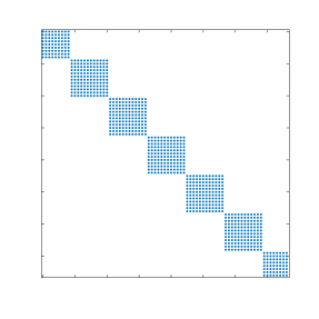
((a)) Test case I: one beam element per fiber

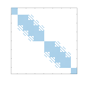
((b)) Test case II: four beam elements per fiber

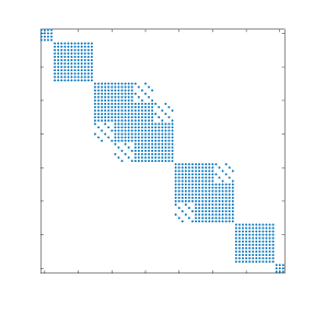
((c)) Test case III: random number (1, 2, 3 or 4) of beam elements per fiber

Figure 4: Partial visualization of the sparsity structure $\mathcal{J}\left(\mathbf{A}\right)$ of matrix $\mathbf{A}$ for test cases I – III

Using SPAIs, the convergence of the linear solver is tightly related to the parameters chosen for the SPAI calculation. In Table 2, different combinations of the drop-off tolerance $\sigma$ and refinement level $\ell$ are given for each of the six test cases. Each value pair represents the largest possible drop-off value $\sigma$ possible for a fixed refinement level $\ell$, such that the linear solver still converges. For certain values of $\ell$, no convergence could be a archived at all for some test cases, even with a very small drop-off tolerance $\sigma$. In these situations, an appropriate value of $\sigma$ is chosen, such that only explicit zero values are dropped from the matrix graph to still be able to make a fair comparison with the other test cases regarding the error norm and number of non-zero entries in the approximate inverse. In addition, the number of non-zero entries of the filtered graph $\underline{\mathcal{J}\left(\mathbf{A}\right)}$ used as starting point for the sparsity pattern construction as well as the amount for the graph of the inverse approximation $\mathcal{J}\left({\mathbf{A}}^{\ast}\right)$ are given. The number of non-zeros for the unfiltered graph, $\mathrm{nnz}\left(\mathcal{J}\left(\mathbf{A}\right)\right)$, is illustrated in Table 1 for comparison. The behavior of the iterative linear solver is assessed by the averaged number of iterations per nonlinear solver step and three timings concerning the preconditioner setup time $T_{\mathrm{setup}}$, the time spent for solving the linear system $T_{\mathrm{solve}}$ and the total time $T_{\mathrm{total}}=T_{\mathrm{setup}}+T_{\mathrm{solve}}$. The overall quality of the inverse approximation ${\mathbf{A}}^{\ast}$ is quantified by the error norm relative to the exact inverse $\mathbf{A}^{-1}$.

Table 2: Comparison of the influence of different values of $\sigma$ and $\ell$ on the number of linear solver iterations and timings

	$\sigma$	$\ell$	$\mathrm{nnz}\left(\underline{\mathcal{J}\left(\mathbf{A}\right)}\right)$	$\mathrm{nnz}\left(\mathcal{J}\left({\mathbf{A}}^{\ast}\right)\right)$	$\#$iter	CPU time ($\unit{}$)			rel. error norm
						$T_{\mathrm{setup}}$	$T_{\mathrm{solve}}$	$T_{\mathrm{total}}$	$\frac{\left\|{\mathbf{A}}^{\ast}-\mathbf{A}^{-1}\right\|_{\mathrm{F}}}{\left\|\mathbf{A}^{-1}\right\|_{\mathrm{F}}}$
Test case I	$10^{-10}$	$1$	$14572$	$14572$	15	$3.755$	$1.059$	$4.814$	$2.100\cdot 10^{-3}$
	$10^{-8}$	$2$	$11576$	$14688$	13	$3.655$	$0.974$	$4.629$	$1.248\cdot 10^{-12}$
	$10^{-6}$	$3$	$9552$	$14688$	13	$3.718$	$0.967$	$4.685$	$1.248\cdot 10^{-12}$
Test case II	$10^{-11}$	$1$	$44335$	$44335$	-	-	-	-	$7.653\cdot 10^{-1}$
	$10^{-10}$	$2$	$37222$	$86861$	13	$3.973$	$1.007$	$4.980$	$6.000\cdot 10^{-12}$
	$10^{-9}$	$3$	$32436$	$91592$	12	$3.975$	$0.914$	$4.889$	$1.981\cdot 10^{-14}$
Test case III	$10^{-12}$	$1$	$26966$	$26966$	50	$3.730$	$3.823$	$7.553$	$1.415\cdot 10^{-1}$
	$10^{-10}$	$2$	$23919$	$35961$	14	$3.775$	$0.930$	$4.705$	$3.433\cdot 10^{-13}$
	$10^{-8}$	$3$	$17544$	$35814$	12	$3.810$	$0.934$	$4.744$	$3.433\cdot 10^{-13}$
Test case IV	$10^{-12}$	$1$	$26662$	$26662$	-	-	-	-	$9.277\cdot 10^{-1}$
	$10^{-11}$	$2$	$26614$	$44978$	13	$4.197$	$1.017$	$5.214$	$1.082\cdot 10^{-12}$
	$10^{-7}$	$3$	$16748$	$42641$	13	$4.038$	$1.028$	$5.066$	$1.081\cdot 10^{-12}$
Test case V	$10^{-12}$	$1$	$92731$	$92731$	-	-	-	-	$9.519\cdot 10^{-1}$
	$10^{-12}$	$2$	$92731$	$249034$	-	-	-	-	$1.528\cdot 10^{-1}$
	$10^{-11}$	$3$	$87453$	$331152$	14	$5.276$	$1.119$	$6.395$	$1.954\cdot 10^{-7}$
Test case VI	$10^{-12}$	$1$	$49614$	$49614$	-	-	-	-	$9.530\cdot 10^{-1}$
	$10^{-12}$	$2$	$49614$	$109705$	-	-	-	-	$5.970\cdot 10^{-2}$
	$10^{-9}$	$3$	$38420$	$121400$	14	$4.920$	$1.135$	$6.055$	$3.829\cdot 10^{-12}$

In test case I, the dense sub-blocks of the block-diagonal sparsity pattern of $\mathbf{A}$ already lead to the exact graph of the inverse, which makes the approximation rather simple. For the given parameter combinations the upper bound of number of non-zeros to exactly compute $\mathbf{A}^{-1}$ is quickly reached resulting in low iteration counts and error norms. For the given problem, the setup timings are nearly identical, with only the solver timings for the first parameter combination taking a bit longer due to a not fully populated sparsity pattern.

The second test case is based on rather sparse sub-blocks of bigger size compared to test case I. Without a pattern refinement, the linear solver did not converge as the approximation quality of the inverse is not sufficient. For higher refinement levels, the number of non-zeros in $\mathcal{J}\left({\mathbf{A}}^{\ast}\right)$ quickly increases resulting in convergence of the method with still acceptable timings. Yet, there is not a lot of flexibility in choosing the drop-off tolerance $\sigma$ to still retain convergence.

As test case III is a combination of the first two problems, the resulting behavior is a mix of these. Using the initial sparsity graph for the inverse approximation results in $50$ linear solver iterations until convergence, which explains the high solving time $T_{\mathrm{solve}}$. On the other hand, the setup time $T_{\mathrm{setup}}$ is comparable to the other tests. For increased refinement levels $\ell$, a similar behavior as in test cases I and II is observed.

For the fourth test case, the beam elements are switched to a Simo–Reissner formulation, which contributes additional rotational degrees of freedom into $\mathbf{A}$. In difference to test case I, this results in already sparse sub-blocks for using one beam element per fiber. Therefore, using just the graph $\mathcal{J}\left(\mathbf{A}\right)$ results in a poor approximation of the sparsity pattern of the inverse and thus leads to no convergence. Using higher refinement levels $\ell$ for the sparse approximate inverse approximation quickly heals this problem and even allows to choose higher values for $\sigma$, i.e., dropping small values.

Test case V and VI show a similar behavior and only converge with $\ell=3$. The additional beam elements used per fiber increase the blocksize of each sub-block and thus leave more room for possible sparse approximations for the inverse. The static approach for choosing an appropriate sparsity pattern for the inverse presented in Section 4.2.3 is still able to produce good approximations, thus leading to convergence of the linear solver, but only for rather dense representations of ${\mathbf{A}}^{\ast}$.

In conclusion, a robust parameter combination is highly problem dependent and necessary to achieve convergence of the linear method. In the presented cases, a refinement level of $\ell=3$ and a drop-off tolerance of $\sigma=10^{-9}$ to get rid of small values polluting the sparsity pattern showed to be sufficient to enable convergence even for challenging cases.

5.2 Weak scaling behavior

To study the performance of the proposed block preconditioner also for large-scale examples and on parallel computing clusters, we now conduct a weak scaling study. The problem setup is similar to test case I from Section 5.1. To guarantee that large problems exhibit the same fiber distribution at least in parts of the domain, the meshes are setup as follows: We first create the geometry and mesh for the largest problem by placing a cube with edge length $\qty{10}{}$ inside a cartesian frame of reference, such that the cube’s center of mass coincides with the origin $O$ and its edges are oriented along the cartesian axes. Then, the cube is filled with randomly positioned and oriented straight fibers with length $l^{\mathcal{B}}=\qty{0.25}{}$ and radius $R=\qty{0.005}{}$. Only fibers, which are fully contained in the cube, are considered. This problem will be solved on 1000 MPI ranks. For smaller problems, the geometry is cut out of this initial cube. Also for the cut out problem, only fully contained fibers are considered. Figure 5 shows the intersections of the series of cubes with each coordinate plane spanned by basis vectors $\bm{e}_{\xi}$ and $\bm{e}_{\eta}$, $\xi,\eta\in\{1,2,3\},\xi\neq\eta$.

Figure 5: Intersections of all cubes (IDs 1 – 9) of the weak scaling studies with planes spanned by basis vectors $\bm{e}_{\xi}$ and $\bm{e}_{\eta}$, $\xi,\eta\in\{1,2,3\},\xi\neq\eta$ in the cartesian frame of reference. Orientation of the cutting planes is sketched in the top left.

This process not only yields an almost constant beam-solid volume ratio for all problem sizes, but also guarantees that larger meshes are just extensions of the smaller meshes. The load per processor is kept constant at around $50k$ degrees of freedom. Meshing details are given in Table 3.

Table 3: Mesh refinement schedule for the weak scaling study

ID	$n^{\mathrm{proc}}$	$n^{S}_{DOF}$	$n^{B}_{DOF}$	$n^{total}_{DOF}$	$n^{total}_{DOF/proc}$
1	8	$397953$	$9132$	$407085$	$50885.6$
2	27	$1316928$	$31824$	$1348752$	$49953.8$
3	64	$3090903$	$74916$	$3165819$	$49465.9$
4	125	$6001128$	$146724$	$6147852$	$49182.8$
5	216	$10328853$	$257448$	$10586301$	$49010.7$
6	343	$16355328$	$413976$	$16769304$	$48890.1$
7	512	$24361803$	$621876$	$24983679$	$48796.2$
8	729	$34629528$	$892932$	$35522460$	$48727.7$
9	1000	$47439753$	$1222320$	$48662073$	$48662.1$

The boundary conditions are identical to test case I from Section 5.1, i.e., the bottom surface is clamped and the top surface loaded with a constant tensile load of $p=\qty{1}{/\square}$. The solid is again modeled by a St.-Venant–Kirchhoff material (Young’s modulus $E^{\mathcal{S}}=\qty{1}{/\square}$, Poisson’s ratio $\nu^{\mathcal{S}}=0.3$) and discretized with first-order hexahedral finite elements. The fibers are modeled using TF beam elements with Young’s modulus $E^{\mathcal{B}}=\qty{10}{/\square}$. The positional coupling condition is enforced with a penalty parameter of ${\epsilon}^{\mathcal{V}}=\qty{10}{/\square}$.

The overall simulation is again of quasi-static nature and imposes the total load over the course of two load steps. The nonlinear solver converges, if the nonlinear residual $\left\|\mathbf{f}\right\|_{2}$ drops below $10^{-6}$ and the full displacement increment $\left\|\Delta\mathbf{d}\right\|_{2}$ is smaller than $10^{-8}$. For the solution of the linear system arising in each nonlinear iteration, a preconditioned GMRES method is applied with the proposed preconditioner. Hereby, the parameters are set as follows: the relaxation factor is kept at $\alpha=1.0$, the number of sweeps through the preconditioner is set to $k=3$ as well as the number of iterations for the SPAI smoother $m=3$. The Schur complement equation is solved with an aggregation-based multigrid. Coarsening is performed until the number of unknowns on the coarsest level drops below 6500. The MG hierarchy is traversed using a V-cycle with level transfer operators arising from either PA-AMG or SA-AMG. On all but the coarsest level, the level smoother is chosen as ILUT with overlap $\delta=1$, fill-in level $p=1$ and drop-off tolerance $\tau=10^{-4}$. The coarse level is solved with a direct solver using the distributed memory version of SuperLU [29]. The outer GMRES solver is assumed to be converged if the relative residual $\left\|\mathbf{r}^{n}\right\|_{2}/\left\|\mathbf{r}^{0}\right\|_{2}$ falls below $10^{-8}$.

The scaling study is run on our in-house cluster (16 nodes with 2x Intel Xeon Cascade Lake CPUs with 26 cores, 20 nodes with 2x Intel Xeon Skylake CPUs with 24 cores, 1312 cores in total, Mellanox Infiniband Interconnect). The overall weak scaling performance is quantified by the averaged number of iterations per nonlinear Newton iteration and the timings for setting up the preconditioner $T_{\mathrm{setup}}$, for solving the linear system $T_{\mathrm{solve}}$ and the total solver time $T_{\mathrm{total}}=T_{\mathrm{setup}}+T_{\mathrm{solve}}$. Since the setup of the preconditioner is expected to be expensive, we also examine the option of reusing the preconditioner throughout all Newton steps of a load step with the aim to reduce $T_{\mathrm{setup}}$ and, thus, also reduce $T_{\mathrm{total}}$.

((a)) Averaged number of GMRES iterations per Newton step

((b)) Setup time $T_{\mathrm{setup}}$

((c)) Solve time $T_{\mathrm{solve}}$

((d)) Total solver time $T_{\mathrm{total}}$

Figure 6: Weak scaling behavior

Figure 6 summarizes the results of the weak scaling study. We first discuss the case, where the preconditioner is built in every Newton step. Looking at the iteration counts in Figure 6(a), the SA-AMG method delivers iteration counts independent of the problem size (with mostly 17 iterations per solve), while PA-AMG exhibits an increase in iterations by a factor of $2\times$ (from 34 to 71 iterations) when increasing the problem size by $120\times$, i.e., from mesh ID 1 to mesh ID 9, cf. Table 3. Regarding the setup time $T_{\mathrm{setup}}$ required to build the preconditioner shown in Figure 6(b), PA-AMG is more than twice as fast as SA-AMG due to the smaller support of PA-AMG interpolation functions and, thus, less fill-in in coarse level operators. In contrast, the time to solve the linear system is more than $2\times$ smaller for SA-AMG due to the better approximation properties of smoothed interpolation functions in SA-AMG, cf. Figure 6(c). When looking at the combined time $T_{\mathrm{total}}=T_{\mathrm{setup}}+T_{\mathrm{solve}}$ as shown in Figure 6(d), both types of transfer operators result in very similar timings.

With a moderate increase of $T_{\mathrm{setup}}$ for PA-AMG for an increasing number of parallel processes, the increase in solver time $T_{\mathrm{solve}}$ as well as total time $T_{\mathrm{total}}$ of the PA-AMG scheme appears to be directly linked to the number of iterations required to achieve the desired tolerance of the iterative linear solver. In contrast, SA-AMG requires a rather constant number of iterations for all problem sizes and spends most of its time in the preconditioner setup, thus resulting in total solver timings $T_{\mathrm{total}}$ that are dominated by the preconditioner setup time. This hints a potential savings when setting up the preconditioner once and then reusing it to solve multiple subsequent linear systems, e.g., through the course of a Newton scheme.

We now look at the option of building the preconditioner only in the first Newton step and then reusing it throughout an entire load step. In the present study, each load step requires two Newton steps, hence we expect to save 50% of $T_{\mathrm{setup}}$ and hope to not worsen in terms of iteration numbers and solver time $T_{\mathrm{solve}}$. When looking at the setup time in Figure 6(b), setup costs for both SA-AMG and PA-AMG are reduced by $\approx 50\%$ as expected. Furthermore, the iteration numbers as well as the solver time $T_{\mathrm{solve}}$ increase only slightly for both SA-AMG and PA-AMG, cf. Figures 6(a) and 6(c). Overall, the reuse of the preconditioner positively impacts the total solver time $T_{\mathrm{total}}$ with the best option being SA-AMG with reuse of the preconditioner, which appears to be roughly $30\%$ faster than the variant without reuse of the preconditioner. We note that the actual benefit of reusing the preconditioner depends on the number of nonlinear solver iterations per load step: The more Newton steps are required, the greater savings are to be expected from reusing the preconditioner.

In conclusion, this example has shown weak scalability of the proposed preconditioner. The iteration numbers remain perfectly constant for SA-AMG. Due to the overlap $\delta=1$ of the ILUT smoother in the MG hierarchy, the setup time $T_{\mathrm{setup}}$ increases by a factor of $\approx 5\times$ when increasing the problem size by $120\times$, i.e., from mesh ID 1 to mesh ID 9, cf. Table 3. We stress that the choice of transfer operators has a great influence on the total weak scalability of the preconditioner. In the presented test cases, the best scalability in terms of the iteration count were obtained by SA-AMG transfer operators and when reusing the preconditioner though all Newton steps of a load step. In sum, SA-AMG appears as the method of choice to demonstrate weak scalability and keep the iteration count low. For more complex application scenarios however, it might be beneficial to fall back to PA-AMG due to its reduced fill-in during coarsening. Given the intricate nature of beam-solid applications and their arising systems of linear equations, we deem the present weak scaling behavior acceptable and adequate.

5.3 Application: Concrete wall with steel reinforcements

To show the applicability of the proposed block preconditioner to real-world problems, we study an example from civil engineering, in particular the loading of a steel-reinforced concrete wall. The problem setup and its dimensions are shown in Figure 7.

((a)) Measurements (unit: $\unit{}$) of the concrete wall with a thickness of $\qty{0.24}{}$

((b)) Concrete wall with steel reinforcements

Figure 7: Geometric configuration of a steel-reinforced concrete wall

Since we are focusing on the performance of the linear solver and the proposed preconditioner, we restrict ourselves in this example to an idealized, fully elastic constitutive behavior of concrete. Therefore, it suffices to model the solid with a St.-Venant–Kirchhoff material ($E^{\mathcal{S}}=\qty{30}{\giga}$, $\nu^{\mathcal{S}}=0.3$). In this study, we, thus, refrain from using more elaborate constitutive models, that also cover inelastic effects, such as the Drucker–Prager model [13], which could serve as a smeared, phenomenological model for concrete undergoing damage or crack initiation. Yet, we study a complex reinforcement design: The initially curved reinforcement bars are modeled as Simo–Reissner beams ($E^{\mathcal{B}}=\qty{210}{\giga}$, $\nu^{\mathcal{B}}=0.0$) with a fiber cross section radius of $R=\qty{0.005}{}$. The bottom and left side of the wall are clamped, restricting the displacement of the solid and fibers. Additionally, a distributed load of $\qty{-3e7}{/\square}$ is applied on the top surface in $\bm{e}_{2}$ direction and $\qty{1.5e5}{/\square}$ on the back surface in $\bm{e}_{3}$ direction. The reinforced concrete wall is discretized with first-order hexahedral finite elements for the solid domain and Simo–Reissner beam elements for the reinforcement fibers, respectively. We study this problem for three different mesh sizes (coarse, medium, fine), where each refinement quadruples the total number of unknowns. Details on these meshes including the resulting number of degrees of freedom for each field are given in Table 4 along with the computational resources, i.e., number of MPI ranks $n^{\mathrm{proc}}$, used for each mesh. The penalty parameters for positional and rotational couplings are set to ${\epsilon}^{\mathcal{V}}=\qty{2.1e11}{/\square}$ and ${\epsilon}^{\mathcal{R}}=\qty{5.25e6}{/}$, respectively. We perform a quasi-static simulation and impose the total load over the course of four load steps.

Exemplarily, Figure 8 depicts the sparsity pattern of the system matrix for the coarse mesh.

Figure 8: Sparsity pattern of the linear system arising from the coarse mesh of the concrete wall (cf. Table 4) with the block-diagonal beam sub-block $\mathbf{A}$ (orange), the solid sub-block $\mathbf{C}$ (white), and the off-diagonal coupling blocks $\mathbf{B}_{1}^{\mathrm{T}}$ and $\mathbf{B}_{2}$ (gray)

The $2\times 2$ blocking as introduced in (8) is highlighted through colors. The beam sub-block $\mathbf{A}$ (orange) internally exhibits block diagonal structure as illustrated in Figure 4, which allows for an efficient construction of the SPAI, since the sparsity pattern of the inverse can be estimated very well based on the block-diagonal structure of $\mathbf{A}$. Arising from the penalty contributions assembled into $\mathbf{C}$, the solid sub-block $\mathbf{C}$ (white) contains many entries far away from its diagonal, exemplifying the attested lack of diagonal dominance, cf. Section 3.2. Both beams and solid are connected through the coupling blocks $\mathbf{B}_{1}^{\mathrm{T}}$ and $\mathbf{B}_{2}$ (gray), which are the main reasons for the loss of block diagonal dominance, again see Section 3.2.

For all simulations, the nonlinear solver converges, if the nonlinear residual $\left\|\mathbf{f}\right\|_{2}$ drops below $10^{-8}$ and the displacement increment $\left\|\Delta\mathbf{d}\right\|_{2}$ falls below $10^{-8}$. To get an idea of the effectiveness of the proposed preconditioner in an application scenario, we compare different methods to solve the arising linear system in each Newton step, in particular a direct solver (by applying the distributed memory version of SuperLU [29]), a GMRES solver with an incomplete LU (ILU) preconditioner, and a GMRES solver with the proposed preconditioner from Section 4. Where applicable, we also study the effect of reusing the preconditioner over multiple invocations of the linear solver within a single load step to better amortize the potentially expensive setup of the block preconditioner. In case of GMRES, we assume convergence of the linear solver, if the full relative residual norm $\left\|\mathbf{r}^{n}\right\|_{2}/\left\|\mathbf{r}^{0}\right\|_{2}$ drops to at least $10^{-6}$.

In case of the block preconditioner, we apply $k=3$ sweeps of the proposed preconditioner within each GMRES iteration. The SPAI computation for the beam sub-matrix $\mathbf{A}$ uses a drop tolerance $\sigma=10^{-8}$ and a refinement level $\ell=4$ to enrich the sparsity pattern. For the predictor step, the described SPAI smoother is applied with $m=3$ sweeps. The Schur complement equation in the correction step is tackled with a plain-aggregation AMG hierarchy with a maximum size of the coarse level problem of 6500 unknowns, which results in three MG levels for all meshes. Prolongator smoothing (as proposed by [56] and usually beneficial for problems in solid mechanics) is explicitly disabled to reduce the fill-in of the coarse level matrices; see [54] for a detailed comparison. An ILUT method with $\delta=1$, $p=2.5$, and $\tau=10^{-4}$ is used as level smoother. The coarse level equations are solved directly using the distributed memory version of SuperLU [29].

The solver options and their iteration counts and timings are summarized in Table 4.

Table 4: Comparison of averaged linear solver timings per nonlinear iteration for a steel-reinforced concrete wall

$n^{\mathrm{proc}}$	$n^{\mathcal{S}}_{DOF}$	$n^{\mathcal{B}}_{DOF}$	$n^{total}_{DOF}$	Method	Reuse	$\#$iter	CPU time ($\unit{}$)			Speedup
							$T_{\mathrm{setup}}$	$T_{\mathrm{solve}}$	$T_{\mathrm{total}}$	$\frac{T_{\mathrm{total}}^{direct}}{T_{\mathrm{total}}^{iterative}}$
8	$180888$	$45894$	$226782$	LU	no	-	1070	2.8	1072.8
				GMRES+ILU	no	no convergence
				GMRES+SIMPLE	no	33	100.0	17.6	117.6	$\approx$ 9
				GMRES+SIMPLE	yes	33	19.0	17.7	36.7	$\approx$ 29
32	$844545$	$45894$	$890439$	LU	no	-	5358	8.3	5366.3
				GMRES+ILU	no	no convergence
				GMRES+SIMPLE	no	33	144.6	24.4	169.0	$\approx$ 32
				GMRES+SIMPLE	yes	34	28.7	24.7	53.4	$\approx$ 100
128	$3323565$	$45894$	$3369459$	LU	no	not feasible
				GMRES+ILU	no	no convergence
				GMRES+SIMPLE	no	30	186.4	26.1	212.5	n/a
				GMRES+SIMPLE	yes	31	36.7	26.1	62.8	n/a

Each of the four load steps requires five Newton iterations to reach convergence of the nonlinear solver. The reported iteration counts and timings have been averaged over all load steps and Newton steps, such that the numbers now give a good estimate for the cost of a single invocation of the linear solver. For the direct solver, the coarse and medium mesh could be solved, while the fine mesh was infeasible, i.e., one load step taking more than three days of wall clock time on a cluster, such that we do not report the final result. For the out-of-the-box iterative solver using a GMRES method preconditioned with an incomplete LU factorization, the iterative solver was not able to reach convergence within 1000 iterations. Only GMRES with the proposed block preconditioner from Section 4 was able to solve all three levels of mesh refinement. Moreover, the iterative method outperforms the direct solver in the sense that it is roughly $9\times$ faster than the direct method for the coarse discretization. When moving to the medium-sized mesh, the discrepancy in solver timings increases even further: the direct method requires a total solver time $T_{\mathrm{total}}=\qty{5366.3}{}$ for a single solve, while total solver time $T_{\mathrm{total}}$ of the preconditioned GMRES only take $\qty{169.0}{}$, resulting in a speed-up of approximately $32\times$. Increasing the problem size even further makes the application of a direct method infeasible, as memory consumption and computing time become prohibitively high, leaving the iterative approach as the sole viable option. In all working cases, the linear iterations for the preconditioned iterative method per Newton step remain almost constant over the whole simulation for each problem and in addition also stay almost constant for each mesh size. For the coarse mesh, approximately $33$ iterations are necessary to achieve the desired tolerance, whereas the medium and large setup require $33$ and $30$ iterations on average, respectively. Still, the discrepancy between $T_{\mathrm{setup}}$ and $T_{\mathrm{solve}}$ is rather large for the iterative method, as most of the computation time is spent in the construction of the factorization of the ILUT level smoother. To better amortize the expensive setup cost, one can build the preconditioner only once per load step and then reuse it for each Newton step with the goal of decreasing the overall simulation time. This shows to be an effective option, as it reduces the setup time $T_{\mathrm{setup}}$ by a factor of $5\times$ in each case, which is perfectly in line with using the preconditioner five times, but only building it once per load step. Due to the reuse, the preconditioner is not perfectly fitting the system matrix anymore, occasionally resulting in a slight increase in iteration numbers (#iter) and solver time $T_{\mathrm{solve}}$. Overall though, the total solver time $T_{\mathrm{total}}$ is reduced, which also manifests itself in the speed-up factors of $29\times$ and $100\times$ in Table 4 for the coarse and medium mesh. The infeasibility of a direct solver for the fine mesh prevents the calculation of a speed-up factor (n/a), however clearly testifies to the beneficial impact of the proposed preconditioner on the solvability of large-scale application examples.

Overall, this example demonstrates not only the applicability of the proposed preconditioner in engineering problems, but also its benefits in terms of efficiency and speed-up, ultimately enabling the analysis of large and complex fiber-solid systems, which have not been accessible with existing linear solvers so far.

6 Concluding remarks

In this paper, we have proposed a physics-based multi-level block preconditioner for the scalable solution of mixed-dimensional models in beam-solid interaction, specifically tailored to systems with many independent fibers being embedded into a solid domain. The regularized mortar-type coupling approach leads to $2\times 2$ block systems exhibiting particular properties, most prominently the lack of block diagonal dominance stemming from the penalty terms on the off-diagonal coupling blocks, which render classical block relaxation preconditioners inapplicable. Following a SIMPLE-type approach to precondition an outer Krylov solver, we utilize an approximate block factorization to enable the tackling of the individual blocks and their coupling within the preconditioner. To this end, we exploit the beam-related sub-block’s sparsity structure resembling a block diagonal matrix to explicitly construct a sparse approximate inverse (SPAI) by solving a minimization problem over the Frobenius norm on a given sparsity pattern, which in practice is decomposed into row-wise minimizations to be solved in parallel. To increase its robustness and approximation quality, the SPAI computation is equipped with pre-processing steps such as a filtering of small entries and a static enrichment of the sparsity pattern as well as a post-filtering of small entries. This approximation has then not only been used for the explicit formation of an approximation to the Schur complement, but also as a smoother in SIMPLE’s prediction step. To solve the Schur complement equation in the correction step, we have employed an AMG hierarchy. Due to the Schur complement’s fill-in stemming from the SPAI matrix as well as the penalty contributions, an ILUT factorization with fill-in $p$, threshold $\tau$, and overlap $\delta$ serves as level smoother on all levels except for the direct solver on the coarse level. All building blocks of the proposed preconditioner have been implemented in Trilinos and are available as open-source software to the entire scientific community.

We have studied the influence of the SPAI algorithm’s parameters and have found, that a static enrichment of the graph $\mathcal{J}\left(\mathbf{A}\right)$ of at least $\ell=2$ greatly improves the quality of the approximation as well as the performance of the iterative solver, while more enrichment might be required for particularly challenging problems. Regarding the scaling behavior, we were able to demonstrate weak scalability up to 1000 MPI ranks. While the iteration count is completely independent of the problem size and number of MPI ranks for SA-AMG, the setup and solver time exhibit a minor increase with an increasing problem size. This is mainly attributed to the use of an ILUT level smoother within SIMPLE’s correction step. Finally, we have investigated an application example from civil engineering, in particular a steel-reinforced concrete wall, and have compared the performance of the proposed multi-level preconditioner to established one-level preconditioners and direct solvers. Even for a coarse mesh, the one-level preconditioner failed to converge. The proposed multi-level preconditioner delivered a speed-up by a factor up to $100\times$ compared to the direct solver on small and medium sized meshes, whereas the application of a direct method on the finest mesh was not feasible anymore, leaving the proposed preconditioned iterative method as the only working option. While intractable for existing solvers, the proposed preconditioner enables the analysis of mixed-dimensional fiber-solid systems with complex reinforcement structures for the first time. Considering computational performance, the option of building the preconditioner only once per load step and then reusing it in every iteration of the nonlinear solver has shown to cut down the setup time $T_{\mathrm{setup}}$ at the expected rate, while still delivering a strong preconditioning effect, such that the convergence of the linear solver is not impeded and the total solver time $T_{\mathrm{total}}$ is reduced significantly.

In future work, the proposed preconditioner and its building blocks can be extended to other types of beam-solid interaction phenomena such as the coupling of beams onto a solid’s surface [49] or the contact between beams and solid bodies [53]. Similarly, other mixed-dimensional multi-physics systems such as fiber-fluid interaction are likely to be amenable to such a methodology. It seems worthwhile to use semi-structured grids to discretize the solid domain, if applicable, which in turn allow to further enhance its computational performance in many application scenarios [31]. Performance and scalability bottlenecks associated with the evaluation of the beam-solid coupling terms on a distributed-memory parallel computing cluster need to be addressed, e.g., following ideas from mortar methods for contact mechanics to improve data locality and load balancing [34].

Data Availability Statement

Building blocks of the AMG preconditioner developed and applied in this study are openly available in Trilinos at https://github.com/trilinos/Trilinos [2]. All other data that support the findings of this study are available from the corresponding author upon reasonable request.

Declaration of Competing Interest

The authors declare that they have no known competing financial interests or personal relationships that could have appeared to influence the work reported in this paper.

References

- [1] BACI: A Comprehensive Multi-Physics Simulation Framework. https://baci.pages.gitlab.lrz.de/website/. Accessed: 2023-07-14.
- [2] The Trilinos Project. https://trilinos.github.io. Accessed: 2023-07-14.
- [3] B. D. Agarwal, L. J. Broutman, and K. Chandrashekhara. Analysis and Performance of Fiber Composites. Wiley, 2017.
- [4] J. Ao, M. Zhou, and B. Zhang. A dual mortar embedded mesh method for internal interface problems with strong discontinuities. International Journal for Numerical Methods in Engineering, 123(22):5652–5681, 2022.
- [5] E. Béchet, N. Moës, and B. I. Wohlmuth. A stable lagrange multiplier space for stiff interface conditions within the extended finite element method. International Journal for Numerical Methods in Engineering, 78(8):931–954, 2009.
- [6] L. Berger-Vergiat, C. A. Glusa, G. Harper, J. J. Hu, M. Mayr, A. Prokopenko, C. M. Siefert, R. S. Tuminaro, and T. A. Wiesner. MueLu User’s Guide. Technical Report SAND2023-12265, Sandia National Laboratories, Albuquerque, NM (USA) 87185, 2023.
- [7] O. Bröker and M. J. Grote. Sparse approximate inverse smoothers for geometric and algebraic multigrid. Applied Numerical Mathematics, 41(1):61–80, 2002.
- [8] L. Chacón. An optimal, parallel, fully implicit Newton–Krylov solver for three-dimensional viscoresistive magnetohydrodynamics. Physics of Plasmas, 15:056103, 2008.
- [9] E. Chow. Parallel implementation and practical use of sparse approximate inverse preconditioners with a priori sparsity patterns. The International Journal of High Performance Computing Applications, 15(1):56–74, 2001.
- [10] E. Chow and A. Patel. Fine-Grained Parallel Incomplete LU Factorization. SIAM Journal on Scientific Computing, 37(2):C169–C193, 2015.
- [11] E. C. Cyr, J. N. Shadid, and R. S. Tuminaro. Teko: A Block Preconditioning Capability with Concrete Example Applications in Navier–Stokes and MHD. SIAM Journal on Scientific Computing, 38(5):S307–S331, 2016.
- [12] N. Dimola, M. Kuchta, K.-A. Mardal, and P. Zunino. Robust Preconditioning of mixed-dimensional PDEs on 3d-1d domains coupled with Lagrange multipliers. preprint on arXiv: https://arxiv.org/abs/2307.08431, 2023.
- [13] D. C. Drucker and W. Prager. Soil mechanics and plastic analysis for limit design. Quarterly of Applied Mathematics, 10(2):157–166, 1952.
- [14] D. Durville. Finite element simulation of textile materials at mesoscopic scale. In Finite element modelling of textiles ans textile composites, Saint Petersburg, 2007.
- [15] H. C. Elman, V. E. Howle, J. N. Shadid, R. Shuttleworth, and R. S. Tuminaro. A taxonomy and comparison of parallel block multi-level preconditioners for the incompressible Navier–Stokes equations. Journal of Computational Physics, 227(3):1790–1808, 2008.
- [16] D. Feingold and R. Varga. Block diagonally dominant matrices and generalizations of the Gershgorin Theorem. Pacific Journal of Mathematics, 12(4):1241–1250, 1962.
- [17] B. Flemisch and B. I. Wohlmuth. Stable Lagrange multipliers for quadrilateral meshes of curved interfaces in 3D. Computer Methods in Applied Mechanics and Engineering, 196(8):1589–1602, 2007.
- [18] M. J. Grote and T. Huckle. Parallel preconditioning with sparse approximate inverses. SIAM Journal on Scientific Computing, 18(3):838–853, 1997.
- [19] N. Hagmeyer, M. Mayr, and A. Popp. A fully coupled regularized mortar-type finite element approach for embedding one-dimensional fibers into three-dimensional fluid flow. International Journal for Numerical Methods in Engineering, published online ahead of print:e7435, 2024.
- [20] N. Hagmeyer, M. Mayr, I. Steinbrecher, and A. Popp. One-way coupled fluid-beam interaction: Capturing the effect of embedded slender bodies on global fluid flow and vice versa. Advanced Modeling and Simulation in Engineering Sciences, 9:9, 2022.
- [21] M. Hautefeuille, C. Annavarapu, and J. E. Dolbow. Robust imposition of Dirichlet boundary conditions on embedded surfaces. International Journal for Numerical Methods in Engineering, 90(1):40–64, 2012.
- [22] M. A. Heroux, R. A. Bartlett, V. E. Howle, R. J. Hoekstra, J. J. Hu, T. G. Kolda, Lehoucq, K. R. Long, R. P. Pawlowski, E. T. Phipps, A. G. Salinger, H. K. Thornquist, R. S. Tuminaro, J. M. Willenbring, A. Williams, and K. S. Stanley. An Overview of the Trilinos Project. ACM Transactions on Mathematical Software, 31(3):397–423, 2005.
- [23] D. Jodlbauer, U. Langer, and T. Wick. Parallel block-preconditioned monolithic solvers for fluid-structure interaction problems. International Journal for Numerical Methods in Engineering, 117(6):623–643, 2019.
- [24] S. Kakaletsis, E. Lejeune, and M. Rausch. The mechanics of embedded fiber networks. Journal of the Mechanics and Physics of Solids, 181:105456, 2023.
- [25] U. Khristenko, S. Schuß, M. Krüger, F. Schmidt, B. Wohlmuth, and C. Hesch. Multidimensional coupling: A variationally consistent approach to fiber-reinforced materials. Computer Methods in Applied Mechanics and Engineering, 382:113869, 2021.
- [26] U. Langer and H. Yang. Robust and efficient monolithic fluid-structure-interaction solvers. International Journal for Numerical Methods in Engineering, 108(4):303–325, 2016.
- [27] B. Lé, G. Legrain, and N. Moës. Mixed dimensional modeling of reinforced structures. Finite Elements in Analysis and Design, 128:1–18, 2017.
- [28] F. Lespagnol, C. Grandmont, P. Zunino, and M. A. Fernandez. A mixed-dimensional formulation for the simulation of slender structures immersed in an incompressible flow. Technical Report 98/2023, MOX Politecnico di Milano, 2023.
- [29] X. S. Li and J. W. Demmel. SuperLU_DIST: A scalable distributed-memory sparse direct solver for unsymmetric linear systems. ACM Transactions on Mathematical Software, 29(2):110–140, 2003.
- [30] K.-A. Mardal and R. Winther. Preconditioning discretizations of systems of partial differential equations. Numerical Linear Algebra with Applications, 18(1):1–40, 2011.
- [31] M. Mayr, L. Berger-Vergiat, P. Ohm, and R. S. Tuminaro. Non-invasive multigrid for semi-structured grids. SIAM Journal on Scientific Computing, 44(4):A2734–A2764, 2022.
- [32] M. Mayr, T. Klöppel, W. A. Wall, and M. W. Gee. A Temporal Consistent Monolithic Approach to Fluid–Structure Interaction Enabling Single Field Predictors. SIAM Journal on Scientific Computing, 37(1):B30–B59, 2015.
- [33] M. Mayr, M. Noll, and M. W. Gee. A hybrid interface preconditioner for monolithic fluid-structure interaction solvers. Advanced Modeling and Simulation in Engineering Sciences, 7:15, 2020.
- [34] M. Mayr and A. Popp. Scalable computational kernels for mortar finite element methods. Engineering with Computers, 39:3691–3720, 2023.
- [35] C. Meier, A. Popp, and W. A. Wall. A locking-free finite element formulation and reduced models for geometrically exact Kirchhoff rods. Computer Methods in Applied Mechanics and Engineering, 290:314–341, 2015.
- [36] C. A. Meier, A. Popp, and W. A. Wall. Geometrically Exact Finite Element Formulations for Slender Beams: Kirchhoff–Love Theory Versus Simo–Reissner Theory. Archives of Computational Methods in Engineering, 26(1):163–243, 2019.
- [37] S. Patankar and D. Spalding. A calculation procedure for heat, mass and momentum transfer in three-dimensional parabolic flows. International Journal of Heat and Mass Transfer, 15(10):1787–1806, 1972.
- [38] E. G. Phillips, H. C. Elman, E. C. Cyr, J. N. Shadid, and R. P. Pawlowski. A Block Preconditioner for an Exact Penalty Formulation for Stationary MHD. SIAM Journal on Scientific Computing, 36(6):B930–B951, 2014.
- [39] E. G. Phillips, J. N. Shadid, E. C. Cyr, H. C. Elman, and R. P. Pawlowski. Block Preconditioners for Stable Mixed Nodal and Edge finite element Representations of Incompressible Resistive MHD. SIAM Journal on Scientific Computing, 38(6):B1009–B1031, 2016.
- [40] A. Popp, M. Gitterle, M. W. Gee, and W. A. Wall. A dual mortar approach for 3D finite deformation contact with consistent linearization. International Journal for Numerical Methods in Engineering, 83(11):1428–1465, 2010.
- [41] M. A. Puso. A 3D mortar method for solid mechanics. International Journal for Numerical Methods in Engineering, 59(3):315–336, 2004.
- [42] M. A. Puso and T. A. Laursen. A mortar segment-to-segment contact method for large deformation solid mechanics. Computer Methods in Applied Mechanics and Engineering, 193(6–8):601–629, 2004.
- [43] M. A. Puso and T. A. Laursen. A mortar segment-to-segment frictional contact method for large deformations. Computer Methods in Applied Mechanics and Engineering, 193(45–47):4891–4913, 2004.
- [44] P. Raghavan and S. Ghosh. A continuum damage mechanics model for unidirectional composites undergoing interfacial debonding. Mechanics of Materials, 37(9):955–979, 2005.
- [45] Y. Saad. Ilut: A dual threshold incomplete lu factorization. Numerical Linear Algebra with Applications, 1(4):387–402, 1994.
- [46] Y. Saad. Iterative Methods for Sparse Linear Systems. SIAM, Philadelphia, PA, USA, 2003.
- [47] Y. Saad and M. H. Schultz. GMRES: A Generalized Minimal Residual Algorithm for Solving Nonsymmetric Linear Systems. SIAM Journal on Scientific and Statistical Computing, 7(3):856–869, 1986.
- [48] M. Sedlacek. Sparse Approximate Inverse for Preconditioning, Smoothing, and Regularization. PhD thesis, Technische Universität München, 2012.
- [49] I. Steinbrecher, N. Hagmeyer, C. Meier, and A. Popp. A consistent mixed-dimensional coupling approach for 1D cosserat beams and 2D solid surfaces. preprint on arXiv: https://arxiv.org/abs/2210.16010, 2022.
- [50] I. Steinbrecher, M. Mayr, M. J. Grill, J. Kremheller, C. Meier, and A. Popp. A mortar-type finite element approach for embedding 1D beams into 3D solid volumes. Computational Mechanics, 66(6):1377–1398, 2020.
- [51] I. Steinbrecher and A. Popp. MeshPy – A general purpose 3D beam finite element input generator. https://imcs-compsim.github.io/meshpy, 2021.
- [52] I. Steinbrecher, A. Popp, and C. Meier. Consistent coupling of positions and rotations for embedding 1D Cosserat beams into 3D solid volumes. Computational Mechanics, 69:701–732, 2022.
- [53] I. S. Steinbrecher. Mixed-dimensional finite element formulations for beam-to-solid interaction. PhD thesis, Universität der Bundeswehr München, 2022.
- [54] S. J. Thomas, S. Ananthan, S. Yellapantula, J. J. Hu, M. Lawson, and M. A. Sprague. A comparison of classical and aggregation-based algebraic multigrid preconditioners for high-fidelity simulation of wind turbine incompressible flows. SIAM Journal on Scientific Computing, 41(5):S196–S219, 2019.
- [55] J. P. Van Doormaal and G. D. Raithby. Enhancements of the simple method for predicting incompressible fluid flows. Numerical Heat Transfer, 7(2):147–163, 1984.
- [56] P. Vaněk, J. Mandel, and M. Brezina. Algebraic Multigrid By Smoothed Aggregation For Second And Fourth Order Elliptic Problems. Computing, 56:179–196, 1996.
- [57] T. A. Wiesner, M. Mayr, A. Popp, M. W. Gee, and W. A. Wall. Algebraic multigrid methods for saddle point systems arising from mortar contact formulations. International Journal for Numerical Methods in Engineering, 122(15):3749–3779, 2021.