Unveiling the Potential of Robustness in Evaluating Causal Inference Models

Abstract

The growing demand for personalized decision-making has led to a surge of interest in estimating the Conditional Average Treatment Effect (CATE). The intersection of machine learning and causal inference has yielded various effective CATE estimators. However, deploying these estimators in practice is often hindered by the absence of counterfactual labels, making it challenging to select the desirable CATE estimator using conventional model selection procedures like cross-validation. Existing approaches for CATE estimator selection, such as plug-in and pseudo-outcome metrics, face two inherent challenges. Firstly, they are required to determine the metric form and the underlying machine learning models for fitting nuisance parameters or plug-in learners. Secondly, they lack a specific focus on selecting a robust estimator. To address these challenges, this paper introduces a novel approach, the Distributionally Robust Metric (DRM), for CATE estimator selection. The proposed DRM not only eliminates the need to fit additional models but also excels at selecting a robust CATE estimator. Experimental studies demonstrate the efficacy of the DRM method, showcasing its consistent effectiveness in identifying superior estimators while mitigating the risk of selecting inferior ones.

1 Introduction

The escalating demand for decision-making has sparked an increasing interest in Causal Inference across various research domains, such as economics (Farrell, 2015; Chernozhukov et al., 2018; Kitagawa & Tetenov, 2018; Abadie et al., 2023), statistics (Wager & Athey, 2018; Li & Wager, 2022; Foster & Syrgkanis, 2023; Kennedy, 2023), healthcare (Zhang et al., 2019; Foster et al., 2011; Qian et al., 2021; Bica et al., 2021; Kinyanjui & Johansson, 2022), and financial application (Bottou et al., 2013; Chu et al., 2021; Huang et al., 2021; Donnelly et al., 2021; Fernández-Loría et al., 2023). The primary goal in personalized decision-making is to quantify the individualized causal effect of a specific treatment (or policy/intervention) on the target outcome. For example, in healthcare, the focus lies in understanding the effect of a medical treatment on a patient’s health status; in economics, the emphasis is on evaluating how a public policy would affect one’s welfare; in the digital market, researchers explore the influence of an E-commerce retailer’s lending strategy on a consumer’s potential consumption. Understanding such causal effects is closely connected with identifying a crucial concept in causal inference, which is known as the Conditional Average Treatment Effect (CATE).

Identifying the CATE in observational studies, however, inevitably faces a significant hurdle: the absence of counterfactual knowledge. According to Rubin Causal Model (Rubin, 2005), the CATE is determined by comparing potential outcomes under different treatment assignments (i.e., treat and control) for the same individual. Nonetheless, in real-world applications, this comparison is unfeasible because we can only observe the potential outcome under the actual treatment (i.e., factual outcome), while the potential outcome under the alternative treatment that was not assigned (i.e., counterfactual outcome) remains unobserved. The unavailability of the counterfactual outcome is widely recognized as the fundamental problem in causal inference (Holland, 1986), making it difficult to accurately determine the true value of the CATE.

The advancement of machine learning (ML) has opened up a promising opportunity to improve the CATE estimation from observational data. Several innovative CATE estimation approaches, such as meta-learners and causal ML models, have been proposed to tackle the fundamental challenge in causal inference and enhance the predictive accuracy of CATE estimates (as discussed in Section 2). Nevertheless, the emergence of a variety of CATE estimation methods presents a new predicament for decision-makers: Given multifarious options for CATE estimators, which estimator should be chosen? Standard model selection procedures, such as cross-validation, are commonly employed to select the desirable model by evaluating each model’s performance on a validation set using metrics like mean square error (MSE). Unfortunately, these procedures cannot be applied to CATE estimator selection due to the inherent fundamental problem in causal inference, i.e., only labels for factual outcomes, but not counterfactual outcomes or CATE, are available in observed data. Therefore, exploring proper metrics for CATE estimator selection remains an essential yet challenging research topic in causal inference.

Recent research has emphasized the significance of model selection for CATE estimators, as highlighted in (Schuler et al., 2018; Curth & Van Der Schaar, 2023; Mahajan et al., 2024). These works have proposed and summarized two types of criteria for CATE estimator selection: plug-in and pseudo-outcome metrics, and their large-scale empirical studies have shown that these metrics, to some extent, are helpful in selecting the optimal CATE estimator. However, there still remain two critical dilemmas when utilizing these metrics for CATE estimator selection. The first dilemma lies in the quandary of determining the form of evaluation metric and its underlying ML algorithm. As discussed in Section 2, there are multiple choices available for metric forms and ML algorithms, yet opting for a specific choice among them can inevitably lead us back to the initial estimator selection problem. The second dilemma is the lack of focus on selecting a robust CATE estimator. Robust estimators are expected to demonstrate the necessary generalizability to the unseen (uncertain) counterfactual distribution while maintaining stable performance across different scenarios. In real-world applications, it can be futile to prioritize a ”stellar” estimator over a robust estimator, because we can never accurately determine the actual best estimator without knowledge of the ground truth CATE.

Contributions. In light of above challenges, we propose a novel Distributionally Robust Metric (DRM) method for CATE estimator selection. The contributions are as follows: (1) We establish a novel upper bound for CATE estimation error (i.e., the PEHE defined in Section 3) in a distributionally robust manner, serving as the foundation for the establishment of DRM. (2) The DRM is a model-free metric that eliminates the need to fit additional models for nuisance parameters or plug-in learners. (3) The DRM is designed to prioritize selecting a robust CATE estimator. (4) We provide finite sample analysis for the proposed distributionally robust value $\hat{\mathcal{V}}(\hat{\tau})$, showing it decays to $\mathcal{V}(\hat{\tau})$ at a rate of $n^{-1/2}$. (5) Experimental results demonstrate the consistent effectiveness of DRM in identifying superior estimators while mitigating the risk of selecting inferior ones.

2 Related Work

CATE estimation.

Recent advancements in ML have emerged as powerful tools for estimating CATE from observational data, and researchers pay particular attention to meta-learners and causal ML models. Existing meta-learners mainly include traditional learners such as S-learner, T-learner, PS-learner, and IPW-learner, as well as new learners such as X-learner (Künzel et al., 2019), DR-learner (Kennedy, 2023; Foster & Syrgkanis, 2023), R-learner (Nie & Wager, 2021), and RA-learner (Curth & van der Schaar, 2021b). The specific details of these meta-learners are stated in Appendix A.1. Additionally, some studies also focus on developing innovative causal ML models for CATE estimation, such as Causal BART (Hahn et al., 2020), Causal Forest (Wager & Athey, 2018; ATHEY et al., 2019; Oprescu et al., 2019), generative models like CEVAE (Louizos et al., 2017) and GANITE (Yoon et al., 2018), representation learning nets including SITE (Yao et al., 2018), TARNet (Shalit et al., 2017), Dragonnet (Shi et al., 2019), FlexTENet (Curth & van der Schaar, 2021a), and HTCE (Bica & van der Schaar, 2022), disentangled learning nets like D²VD (Kuang et al., 2017, 2020), DeR-CFR (Wu et al., 2022), and DR-CFR (Hassanpour & Greiner, 2019), and representation balancing nets such as BNN (Johansson et al., 2016), CFRNet (Shalit et al., 2017), DKLITE (Zhang et al., 2020), IGNITE (Guo et al., 2021), BWCFR (Assaad et al., 2021), and DRRB (Huang et al., 2023). Recent surveys (Guo et al., 2020; Yao et al., 2021; Nogueira et al., 2022) have also conducted a systematic review of various causal inference methods.

CATE estimator selection.

Compared to the diverse range of CATE estimation methods, selecting CATE estimators has received limited attention in existing causal inference research. Current methods for selecting CATE estimators can be broadly classified into two main categories. The first category, which is also considered in this paper, involves using plug-in and pseudo-outcome methods to evaluate CATE estimators. These methods share two common characteristics: 1) Both methods require fitting new ML models on a validation set and then implementing the learned ML models in either the plug-in surrogate or the pseudo-outcome surrogate; 2) Both methods serve as surrogates for the expected error between the CATE estimator and the true CATE, i.e., $\mathcal{R}^{oracle}(\hat{\tau})$ in equation (1). The difference between the two methods is that the plug-in method directly approximates the true CATE function, where only covariate variables are involved, while the pseudo-outcome method typically constructs a specific formula incorporating covariates, treatment, and outcome variables. Recent research (Schuler et al., 2018; Curth & Van Der Schaar, 2023; Mahajan et al., 2024) has conducted thorough empirical investigations into the utilization of these two methods for selecting CATE estimators. Their findings suggest that no single selection criterion can universally outperform others in all scenarios in the task of selecting CATE estimators. Particularly, Curth & Van Der Schaar provide valuable insights into the advantages and disadvantages of different plug-in and pseudo-outcome metrics, highlighting the need to further explore CATE estimator selection methods. More details of the two selection methods are stated in Appendix A.2. The second category considers leveraging the data generating process (DGP) to generate synthetic data with a known true CATE, allowing the validation of CATE estimators’ performance on this synthetic data. For example, Advani et al. find that placebo and structured empirical Monte Carlo methods are helpful for estimator selection under some restrictive conditions. Schuler et al.; Athey et al.; Parikh et al. focus on training generative models to enforce the generated data to approximate the distribution of the observed data. However, the DGP-based method still faces some limitations in CATE estimator selection due to two key factors: i) it only guarantees the resemblance of the generated data to the factual distribution, without considering the counterfactual distribution, and ii) there is a potential risk of the method favoring estimators that closely resemble the generative models (Curth et al., 2021).

3 Background

3.1 Preliminary

Notations. Suppose the observational data contain $n$ i.i.d. samples $\{(x_{i},t_{i},y_{i})\}_{i=1}^{n}$, with the associated random variables being $\{(X_{i},T_{i},Y_{i})\}_{i=1}^{n}$. For each unit $i$, $X_{i}\in\mathcal{X}\subset\mathbb{R}^{d}$ is $d$-dimensional covariates and $T_{i}\in\{0,1\}$ is the binary treatment. Potential outcomes for treat ($T=1$) and control ($T=0$) are denoted by $Y^{1},Y^{0}\in\mathcal{Y}\subset\mathbb{R}$. The propensity score (Rosenbaum & Rubin, 1983) is defined as $\pi(x):=P(T=1\mid X=x)$. The conditional mean potential outcome surface is defined as $\mu_{t}(x):=\mathbb{E}\left[Y^{t}\mid X=x\right]$ for $t\in\{0,1\}$. The true CATE is defined as

$$\tau_{true}(x):=\mathbb{E}\left[Y^{1}-Y^{0}\mid X=x\right]=\mu_{1}(x)-\mu_{0}(x).$$

Following the standard and necessary assumptions in potential outcome framework (Rubin, 2005), we impose Assumption 3.1 that ensure treatment effects are identifiable.

Assumption 3.1 (Consistency, Overlap, and Unconfoundedness).

Consistency: If the treatment is $t$, then the observed outcome $Y$ equals $Y^{t}$. Overlap: The propensity score is bounded away from $0$ to $1$, i.e., $0<\pi(x)<1$, $\forall x\in\mathcal{X}$. Unconfoundedness: $Y^{t}\perp\!\!\!\perp T\mid X,\;\forall t\in\{0,1\}$.

3.2 CATE Estimator Selection

The goal of CATE estimator selection is to identify the best CATE estimator, denoted by $\hat{\tau}_{best}$, from a set of $J$ candidate estimators $\{\hat{\tau}_{1},\dots,\hat{\tau}_{J}\}$. The best estimator should satisfy $\hat{\tau}_{best}=\mathop{\arg\min}_{\hat{\tau}\in\{\hat{\tau}_{1},\dots,\hat{\tau}_{J}\}}\mathcal{R}^{oracle}(\hat{\tau})$ such that

$$\mathcal{R}^{oracle}(\hat{\tau}):=\sqrt{\frac{1}{n}\sum_{i=1}^{n}(\hat{\tau}(X_{i})-\tau_{true}(X_{i}))^{2}}.$$ (1)

Here, $\mathcal{R}^{oracle}(\hat{\tau})$ is associated with $\mathbb{E}[(\hat{\tau}(X)-\tau_{true}(X))^{2}]$, which is known as the Precision of Estimating Heterogeneous Effects (PEHE) w.r.t. estimator $\hat{\tau}$ (Hill, 2011; Shalit et al., 2017). Regrettably, due to the unavailability of $\tau_{true}$, $\mathcal{R}^{oracle}(\hat{\tau})$ merely serves as an oracle metric that cannot be utilized to evaluate CATE estimators’ performances in real applications. Previous studies have introduced alternative plug-in and pseudo-outcome metrics to tackle this challenge for selecting CATE estimators. In the following, we will provide an overview of these two metrics.

One can establish a plug-in estimator $\tilde{\tau}$ or construct a pseudo-outcome estimator $\tilde{Y}$ using the validation data. Then, an estimator can be selected based on the following two criteria: $\hat{\tau}_{select}=\mathop{\arg\min}_{\hat{\tau}\in\{\hat{\tau}_{1},\dots,\hat{\tau}_{J}\}}\mathcal{R}_{\tilde{\tau}}^{plug}(\hat{\tau})$ or $\hat{\tau}_{select}=\mathop{\arg\min}_{\hat{\tau}\in\{\hat{\tau}_{1},\dots,\hat{\tau}_{J}\}}\mathcal{R}_{\tilde{Y}}^{pseudo}(\hat{\tau})$ such that

$$\mathcal{R}_{\tilde{\tau}}^{plug}(\hat{\tau})=\sqrt{\frac{1}{n}\sum_{i=1}^{n}(\hat{\tau}(X_{i})-\tilde{\tau}(X_{i}))^{2}},$$ (2)

$$\mathcal{R}_{\tilde{Y}}^{pseudo}(\hat{\tau})=\sqrt{\frac{1}{n}\sum_{i=1}^{n}(\hat{\tau}(X_{i})-\tilde{Y}_{i})^{2}}.$$ (3)

Notably, both the plug-in and pseudo-outcome metrics necessitate the fitting of nuisance parameters $\tilde{\eta}$ (e.g., $\tilde{\eta}=(\tilde{\mu}_{1},\tilde{\mu}_{0},\tilde{\pi})$) using off-the-shelf ML models. Once $\tilde{\eta}$ is obtained, we can proceed to establish $\tilde{\tau}$ and $\tilde{Y}$. For the plug-in metric, $\tilde{\tau}$ can be constructed using any CATE estimator discussed in Appendix A.1, yielding various metrics such as plug-T, plug-DR, etc. For instance, the T-learner can be employed to create the plug-in estimator $\tilde{\tau}(X)=\tilde{\mu}_{1}(X)-\tilde{\mu}_{0}(X)$, which can be further compared with the candidate estimator $\hat{\tau}$ on the validation dataset using equation (2). This is referred to as the plug-T metric. Regarding the pseudo-outcome metric, $\tilde{Y}$ can be constructed using a specific formula discussed in Appendix A.2, yielding various metrics such as pseudo-DR, pseudo-R, etc. For instance, the doubly robust (DR) formula establishes $\tilde{Y}=\tilde{\mu}_{1}(X)-\tilde{\mu}_{0}(X)+\frac{T}{\tilde{\pi}(X)}(Y-\tilde{\mu}_{1}(X))-\frac{1-T}{1-\tilde{\pi}(X)}(Y-\tilde{\mu}_{0}(X))$, which can be further compared with the candidate estimator $\hat{\tau}$ on the validation dataset using equation (3). This is referred to as the pseudo-DR metric. Note that in line with (Curth & Van Der Schaar, 2023), the evaluation metrics based on the influence function (Alaa & Van Der Schaar, 2019) and the R-learner objective (Nie & Wager, 2021) are categorized into the pseudo-outcome metric.

Challenges.

However, the aforementioned CATE estimator selection criteria, the plug-in metric and the pseudo-outcome metric, encounter two crucial dilemmas:

The first dilemma lies in determining the metric form and selecting the underlying ML models. As previously discussed, plug-in metrics have various forms such as plug-T, as do pseudo-outcome metrics such as pseudo-DR. However, studies like (Mahajan et al., 2024) have demonstrated that no single metric form is a global winner, leaving the choice of metric form an open problem. Additionally, both plug-in and pseudo-outcome metrics rely on estimating new nuisance parameters $\tilde{\eta}$ using ML algorithms such as linear models, tree-based models, etc. Plug-in metrics even need to fit an additional ML model for the plug-in learner $\tilde{\tau}$. However, without prior knowledge of the true data generating process, choosing appropriate ML algorithms from the plethoric options can be exceedingly challenging. Consequently, the quandary of determining the metric form and underlying ML model brings us back to the original estimator selection problem (Curth & Van Der Schaar, 2023).

The second dilemma is that these metrics are not well-targeted for selecting a robust CATE estimator. Since the counterfactual distribution is inherently unobservable, models trained on observed factual data cannot guarantee their suitability for unobserved counterfactual data, leading to uncertainty in CATE estimates. Given the crucial role of causal inference in decision-making, the desiderata for a robust estimator that exhibits generalizability to the unseen counterfactual distribution and maintains stable performance across different scenarios becomes paramount in real applications. This need even outweighs the pursuit of an ideal “stellar” estimator because we can never know which estimator is truly superb without access to counterfactual labels.

In light of these challenges, we aim to explore an evaluation metric for selecting CATE estimators that fulfills the following two requirements: (1) The metric should be model-free, eliminating the need for additional model learning for nuisance parameters or plug-in learners. (2) The metric should possess the ability to measure the robustness of a CATE estimator. Interestingly, the PEHE upper bound in representation balancing literature (Shalit et al., 2017; Johansson et al., 2022) meets these two requirements. In the following discussion, we will provide a brief overview of how the PEHE upper bound can be utilized as a heuristic for selecting CATE estimators.

3.3 CATE Estimator Selection: Inspiration from the PEHE Upper Bound in Representation Balancing

Consider a function $h(\Phi(X),t)$ that estimates $Y^{t}$, where $\Phi$ is a representation encoder. According to (Shalit et al., 2017; Johansson et al., 2022), the PEHE w.r.t. $(h,\Phi)$ can be upper bounded by the error in factual outcomes and the distance between the treat and control representations:

$$\epsilon_{PEHE}(h,\Phi) \leq 2\big{(}\epsilon_{F}^{T=1}(h,\Phi)+\epsilon_{F}^{T=0}(h,\Phi)$$ (4)

$$\quad+B_{\Phi}\cdot Dist(P^{T}_{\Phi},P^{C}_{\Phi})-2\sigma^{2}_{Y}\big{)}.$$

More details of this bound are provided in Appendix A.3. Equation (4) intuitively offers a natural approach for selecting a CATE estimator: the ideal estimator should be the one that achieves the smallest upper bound value among all candidate estimators. The underlying rationale is rooted in the insight that reducing the upper bound can theoretically result in a lower PEHE (Shalit et al., 2017; Johansson et al., 2022). However, using equation (4) for CATE estimator selection poses two challenges. Firstly, this upper bound is specifically designed for selecting representation balancing models, rather than generic CATE estimators. Secondly, it cannot be utilized for selecting direct CATE learners since it requires estimating two potential outcome surfaces. Motivated by the insights gained from the upper bound and aiming to address the aforementioned challenges, we will present a new upper bound for PEHE in the forthcoming section. This novel bound not only enables the selection of general CATE estimators but also satisfies the two requirements discussed in Section 3.2.

4 Method

In this section, we propose a novel Distributionally Robust Metric (DRM) method for CATE estimator selection. We begin by outlining the construction of a new PEHE upper bound in a distributionally robust manner in Section 4.1. Subsequently, we establish the DRM based on this novel upper bound in Section 4.2.

4.1 Deriving the PEHE Upper Bound

In equation (4), the PEHE is bounded by the factual error and distributional distance between treat and control representations, while we bound the PEHE in a distinct way. To establish the bound stated in Corollary 4.3, we first bound the PEHE using the following Proposition 4.1.

Proposition 4.1.

The PEHE w.r.t. the CATE estimator $\hat{\tau}$ satisfies the following inequality:

$$\mathbb{E}[(\hat{\tau}(X)-\tau_{true}(X))^{2}]\leq 2\left(\mathbb{E}[(\hat{\tau}(X)-Y^{1})^{2}]+\zeta\right),$$ (5)

where

$$\zeta=\mathbb{V}[\mu_{1}(X)]-\mathbb{V}[Y^{1}]+\mathbb{V}[\mu_{0}(X)]+(\mathbb{E}[\mu_{0}(X)])^{2}.$$

The proof is deferred to Appendix B.1.

Proposition 4.1 indicates that the PEHE can be upper bounded by two terms, $\mathbb{E}[(\hat{\tau}(X)-Y^{1})^{2}]$ and $\zeta$, where $\zeta$ is the sum of four constants that are independent of $\hat{\tau}$. Further, we decompose the term $\mathbb{E}[(\hat{\tau}(X)-Y^{1})^{2}]$ as follows:

$$\mathbb{E}[(\hat{\tau}(X)-Y^{1})^{2}]$$

$$=\underbrace{\mathbb{E}[(\hat{\tau}(X)-Y^{1})^{2}|T=1]}_{\text{Empirically computable}}P(T=1)$$ (6)

$$+\underbrace{\mathbb{E}[(\hat{\tau}(X)-Y^{1})^{2}|T=0]}_{\text{Empirically uncomputable}}P(T=0).$$ (7)

Equation (6) can be computed empirically since the potential outcome $Y^{1}$ is observable in treat samples. However, equation (7) is empirically uncomputable due to the unavailability of $Y^{1}$ in control samples. Our objective now is to establish an upper bound for the uncomputable term $\mathbb{E}[(\hat{\tau}(X)-Y^{1})^{2}|T=0]$. To achieve this, we first define an ambiguity set based on the Kullback-Leibler (KL) divergence in Definition 4.2.

Definition 4.2 (KL ambiguity set).

Given two distributions $Q$ and $P$, let the ambiguity radius $\epsilon>0$ quantify the magnitude of distribution shifts of $Q$ relative to $P$. The KL ambiguity (uncertainty) set $\mathcal{B}_{\epsilon}(P)$ is defined as

$$\quad\quad\quad\quad\mathcal{B}_{\epsilon}(P):=\{Q:D_{KL}(Q||P)\leq\epsilon\},$$ (8)

$$\text{where}\ \quad D_{KL}(Q||P)=\int_{\mathcal{X}}q(x)\log\frac{q(x)}{p(x)}dx$$

denotes the KL divergence, measuring the difference of the arbitrary distribution $Q$ from the reference distribution $P$.

Now we can bound $\mathbb{E}[(\hat{\tau}(X)-Y^{1})^{2}|T=0]$. Define $P^{T}:=P(X,Y^{1}|T=1)$ and $P^{C}:=P(X,Y^{1}|T=0)$ for notational simplicity. By setting an adequately large ambiguity radius in Definition 4.2, the quantity $\mathbb{E}^{P^{C}}[(\hat{\tau}(X)-Y^{1})^{2}]$ in equation (7) satisfies

$$\mathbb{E}^{P^{C}}[(\hat{\tau}(X)-Y^{1})^{2}]\leq\mathcal{V}(\hat{\tau}),$$ (9)

where $$\mathcal{V}(\hat{\tau}):=\sup_{Q\in B_{\epsilon}(P^{T})}\mathbb{E}^{Q}[(\hat{\tau}(X)-Y^{1})^{2}].$$

Equation (9) reveals that the quantity $\mathbb{E}^{P^{C}}[(\hat{\tau}(X)-Y^{1})^{2}]$ can be upper bounded by $\mathcal{V}(\hat{\tau})$, which represents the distributionally robust (worst-case) value of $\mathbb{E}[(\hat{\tau}(X)-Y^{1})^{2}]$ over the uncertainty set $B_{\epsilon}(P^{T})$. The intuition behind this is: since the target distribution $P^{C}$ is unavailable, we can construct an ambiguity set centered around the available reference distribution $P^{T}$, such that the ambiguity set is large enough to contain the unavailable target distribution $P^{C}$. By doing so, we can ensure that the value of the uncomputable quantity $\mathbb{E}^{P^{C}}[(\hat{\tau}(X)-Y^{1})^{2}]$ will be at most $\mathcal{V}(\hat{\tau})$.

As the value $\mathcal{V}(\hat{\tau})$ indicates as a distributionally robust (worst-case) performance, it can naturally measure the robustness of the CATE estimator $\hat{\tau}$ against distributional shifts from the reference distribution $P^{T}$ to the deployment distribution $Q$. Consequently, we can obtain the PEHE upper bound based on this distributionally robust value (or worst-case value) $\mathcal{V}(\hat{\tau})$, which is presented in Corollary 4.3.

Corollary 4.3.

Let $\mathcal{V}(\hat{\tau})$ be the quantity defined in equation (9), $\zeta$ be the constant given in Proposition 4.1, and $u:=P(T=1)$. The PEHE w.r.t. $\hat{\tau}$ can be upper bounded by

$$\mathbb{E}[(\hat{\tau}(X)-\tau_{true}(X))^{2}]$$ (10)

$$\leq 2(u\mathbb{E}^{P^{T}}[(\hat{\tau}(X)-Y^{1})^{2}]+(1-u)\mathcal{V}(\hat{\tau})+\zeta).$$

4.2 Establishing Distributionally Robust Metric

In this section, we will present the specific details involved in constructing DRM based on Corollary 4.3. The construction process can be summarized in three steps.

Step 1: Establishing computational tractability of $\mathcal{V}(\hat{\tau})$.

The primal problem in equation (9) is infinite-dimensional, posing a computational challenge. To overcome this, we can reformulate the primal problem to a feasible finite-dimensional problem, as demonstrated in Theorem 4.4.

Theorem 4.4.

The distributionally robust value $\mathcal{V}(\hat{\tau})$ in equation (9) is equivalent to

$$\mathcal{V}(\hat{\tau})=\min_{\lambda>0}\lambda\epsilon+\lambda\log\mathbb{E}^{P^{T}}[\exp((\hat{\tau}(X)-Y^{1})^{2}/\lambda)].$$ (11)

The proof is deferred to Appendix B.3.

Based on finite sample data, the corresponding empirical estimate $\mathcal{V}(\hat{\tau})$ can be obtained as follows:

$$\hat{\mathcal{V}}(\hat{\tau})=\min_{\lambda>0}\lambda\epsilon+\lambda\log\frac{1}{n_{t}}\sum_{i=1}^{n}T_{i}\exp((\hat{\tau}(X_{i})-Y_{i})^{2}/\lambda).$$ (12)

Note that in equation (12), the potential outcome $Y^{1}$ is replaced by the observed outcome $Y$ because the summation is over treat samples, which follows the Consistency assumption in Assumption 3.1. Since we use $\mathcal{V}(\hat{\tau})$ to approximate $\mathcal{V}(\hat{\tau})$ based on observational data, it is also necessary to provide a finite sample analysis of the gap between $\hat{\mathcal{V}}(\hat{\tau})$ and $\mathcal{V}(\hat{\tau})$. In the following Theorem 4.5, we demonstrate that $|\hat{\mathcal{V}}(\hat{\tau})-\mathcal{V}(\hat{\tau})|$ decays at a rate of $n^{-1/2}$.

Theorem 4.5.

Let $u:=P(T=1)$. Assume $0<\underaccent{\bar}{\lambda}\leq\lambda\leq\bar{\lambda}$ and $(\hat{\tau}(X)-Y)^{2}$ is bounded within the range of $\underaccent{\bar}{M}$ to $\bar{M}$. For $n\geq 2/u^{2}\log(2/\delta)$, with probability $1-\delta$, we have

$$|\hat{\mathcal{V}}(\hat{\tau})-\mathcal{V}(\hat{\tau})|\leq\mathcal{O}\left(\sqrt{\frac{2\bar{\lambda}^{2}\log(2/\delta)}{nu^{2}}}\right)$$ (13)

$$\quad+\mathcal{O}\left(\sqrt{\frac{8\bar{\lambda}^{2}\log\frac{2}{\delta}}{nu^{2}}\left(\exp(\bar{M}/\underaccent{\bar}{\lambda}-\underaccent{\bar}{M}/\bar{\lambda})\right)^{2}}\right).$$

The proof is deferred to Appendix B.4.

Step 2: Determining the ambiguity radius $\epsilon$.

The ambiguity radius $\epsilon$ plays a critical role in real-world applications (Mohajerin Esfahani & Kuhn, 2018; Ma et al., 2020; Pflug, 2023). However, determining an appropriate value for $\epsilon$ can be challenging as it requires striking a balance between ensuring the bound in equation (9) holds and maintaining its tightness. Specifically, if $\epsilon$ is set too small, it fails to guarantee that the target distribution $P^{C}$ is contained within the ball $\mathcal{B}_{\epsilon}(P^{T})$ (the bound in equation (9) does not necessarily hold). On the other hand, if $\epsilon$ is set too large, even though the ball $\mathcal{B}_{\epsilon}(P^{T})$ can encompass more distributions to ensure the target distribution $P^{C}$ is contained (the bound in equation (9) holds), the bound becomes less tight. Ideally, the radius should satisfy $\epsilon^{*}=D_{KL}(P^{C}||P^{T})$, which ensures that the bound holds and is tight. However, in observational data, calculating $D_{KL}(P^{C}||P^{T})$ is unattainable due to the unseen nature of the target distribution $P^{C}$.

In this paper, instead of directly pursuing $P^{C}$, we present an intriguing alternative approach to acquire $D_{KL}(P^{C}||P^{T})$ through the following Proposition 4.6.

Proposition 4.6.

Let $P^{T}_{X}:=P(X|T=1)$ and $P^{C}_{X}:=P(X|T=0)$ denote the distribution of covariates in the treat and control group, respectively. Assuming that random variables $(X,T,Y^{1},Y^{0})$ satisfy Assumption 3.1, we have

$$D_{KL}(P^{C}||P^{T})=D_{KL}(P^{C}_{X}||P^{T}_{X}).$$ (14)

The proof is deferred to Appendix B.2.

Proposition 4.6 provides an important insight into the relationship between the uncomputable term $D_{KL}(P^{C}||P^{T})$ and a computable quantity $D_{KL}(P^{C}_{X}||P^{T}_{X})$, where $P^{C}_{X}$ and $P^{T}_{X}$ are empirically observable. As a result, we can determine the optimal radius by setting $\epsilon^{*}=D_{KL}(P^{C}_{X}||P^{T}_{X})$.

Step 3: Finalizing Distributionally Robust Metric.

We first define two functions that are useful in obtaining $\mathcal{V}(\hat{\tau})$:

$$\begin{split}&\hat{F}(\lambda,\epsilon;\hat{\tau})=\lambda\epsilon+\lambda\log\frac{1}{n_{t}}\sum_{i=1}^{n}T_{i}e^{\frac{Z_{i}}{\lambda}};\end{split}$$ (15a)

$$\begin{split}&\frac{\partial\hat{F}(\lambda,\epsilon;\hat{\tau})}{\partial\lambda}=\epsilon+\log\sum_{i=1}^{n}\frac{T_{i}e^{\frac{Z_{i}}{\lambda}}}{n_{t}}-\frac{\sum_{i=1}^{n}T_{i}Z_{i}e^{\frac{Z_{i}}{\lambda}}}{\lambda\sum_{i=1}^{n}T_{i}e^{\frac{Z_{i}}{\lambda}}}.\end{split}$$ (15b)

Here, $Z$ denotes $(\hat{\tau}(X)-Y)^{2}$ for notational simplicity. Furthermore, we obtain $\hat{\epsilon}^{*}$ by empirically approximating the KL divergence $D_{KL}(P^{C}_{X}||P^{T}_{X})$ using the Nearest-Neighbor algorithm (Wang et al., 2006; Noh et al., 2014). We then use the Newton-Raphson method to find the empirical solution for $\mathcal{\hat{V}}(\hat{\tau})$, exploiting the convexity of $\hat{F}(\lambda,\epsilon;\hat{\tau})$ w.r.t. $\lambda$. Finally, a CATE estimator can be selected based on the PEHE upper bound value in Corollary 4.3, which corresponds to $\hat{\tau}_{select}=\mathop{\arg\min}_{\hat{\tau}\in\{\hat{\tau}_{1},\dots,\hat{\tau}_{J}\}}\mathcal{R}^{DRM}(\hat{\tau})$ such that

$$\mathcal{R}^{DRM}(\hat{\tau})=\sqrt{\frac{1}{n}\sum_{i=1}^{n}T_{i}(\hat{\tau}(X_{i})-Y_{i})^{2}+\mathcal{\hat{V}}(\hat{\tau})\frac{n_{c}}{n}}.$$ (16)

The complete algorithm of using the DRM method for CATE estimator selection is presented in Algorithm 1.

Algorithm 1 Using DRM for CATE Estimator Selection

0:  The candidate CATE estimators $\{\hat{\tau}_{1},\dots,\hat{\tau}_{J}\}$. The validation dataset with $n$ i.i.d. observational samples $\{(X_{i},T_{i},Y_{i})\}_{i=1}^{n}$. The number of iterations $K$. The initialization $\lambda_{0}$.

1:  Compute $\hat{\epsilon}^{*}=D_{KL}(\hat{P}^{C}_{X}||\hat{P}^{T}_{X})$, with $\hat{P}^{C}_{X}$ and $\hat{P}^{T}_{X}$ being the empirical distributions of $P^{C}_{X}$ and $P^{T}_{X}$, respectively.

2:  for $j=1$ to $J$ do

3:     for $k=0$ to $K-1$ do

4:        Compute $\hat{F}(\lambda_{k},\hat{\epsilon}^{*};\hat{\tau}_{j})$ by equation (15a).

5:        Compute $\partial\hat{F}(\lambda_{k},\hat{\epsilon}^{*};\hat{\tau}_{j})/\partial\lambda_{k}$ by equation (15b).

6:        Compute the update using $\lambda_{k+1}=\max\{\lambda_{k}-\hat{F}(\lambda_{k},\hat{\epsilon}^{*};\hat{\tau}_{j})/(\partial\hat{F}(\lambda_{k},\hat{\epsilon}^{*};\hat{\tau}_{j})/\partial\lambda_{k}),\lambda_{0}\}$.

7:        Save $\hat{\mathcal{V}}(\hat{\tau}_{j})[k]=\hat{F}(\lambda_{k+1},\hat{\epsilon}^{*};\hat{\tau}_{j})$.

8:     Return $\hat{\mathcal{V}}(\hat{\tau}_{j})=\arg\min_{k\in\{0,\dots,K-1\}}\hat{\mathcal{V}}(\hat{\tau}_{j})[k]$.

9:     Use $\hat{\mathcal{V}}(\hat{\tau}_{j})$ to compute $\mathcal{R}^{DRM}(\hat{\tau}_{j})$ by equation (16).

9:  $\hat{\tau}_{select}=\mathop{\arg\min}_{\hat{\tau}\in\{\hat{\tau}_{1},\dots,\hat{\tau}_{J}\}}\mathcal{R}^{DRM}(\hat{\tau})$.

5 Experiments

Table 1: Comparison of different selectors across Settings A, B, and C. Reported values (mean $\pm$ standard deviation) are computed over 100 experiments. Bold denotes the best result among all selectors. $\sqrt{\text{PEHE}}$ & Regret: Smaller is better. Rank correlation: Larger is better.

width 1.88pt   Criterion	$\sqrt{\text{PEHE}}$ (with $\mathcal{R}^{oracle}(\hat{\tau}_{best})$ provided)			Regret			Rank Correlation   width 1.88pt
width 1.88pt   Setting	A (0.24$\pm$0.04)	B (15.49$\pm$1.84)	C (16.10$\pm$2.49)	A	B	C	A	B	C   width 1.88pt
width 1.88pt   Plug-S	29.07$\pm$5.36	27.92$\pm$5.28	35.11$\pm$6.72	122.99$\pm$32.59	0.80$\pm$0.25	1.20$\pm$0.37	-0.14$\pm$0.17	0.75$\pm$0.07	0.71$\pm$0.04   width 1.88pt
width 1.88pt   Plug-PS	29.35$\pm$5.39	28.41$\pm$5.13	36.00$\pm$5.98	124.20$\pm$32.87	0.83$\pm$0.23	1.26$\pm$0.32	-0.17$\pm$0.17	0.74$\pm$0.07	0.70$\pm$0.04   width 1.88pt
width 1.88pt   Plug-T	13.64$\pm$4.00	25.76$\pm$5.21	17.73$\pm$5.09	57.17$\pm$19.76	0.67$\pm$0.29	0.11$\pm$0.33	0.79$\pm$0.11	0.81$\pm$0.06	0.85$\pm$0.04   width 1.88pt
width 1.88pt   Plug-X	18.82$\pm$9.45	25.02$\pm$6.21	31.56$\pm$8.53	79.78$\pm$44.55	0.61$\pm$0.35	0.98$\pm$0.51	0.57$\pm$0.19	0.84$\pm$0.07	0.77$\pm$0.05   width 1.88pt
width 1.88pt   Plug-IPW	29.12$\pm$3.49	61.01$\pm$12.28	63.48$\pm$17.82	123.27$\pm$27.76	2.93$\pm$0.54	2.96$\pm$1.00	0.16$\pm$0.16	0.32$\pm$0.10	0.40$\pm$0.12   width 1.88pt
width 1.88pt   Plug-DR	13.63$\pm$4.32	23.72$\pm$5.58	17.36$\pm$5.25	57.02$\pm$20.43	0.54$\pm$0.32	0.08$\pm$0.30	0.79$\pm$0.11	0.85$\pm$0.07	0.85$\pm$0.04   width 1.88pt
width 1.88pt   Plug-R	37.89$\pm$5.12	159.18$\pm$21.16	164.11$\pm$21.59	160.73$\pm$37.79	9.27$\pm$0.52	9.30$\pm$1.23	-0.54$\pm$0.14	-0.46$\pm$0.08	-0.51$\pm$0.05   width 1.88pt
width 1.88pt   Plug-RA	13.72$\pm$4.24	23.97$\pm$5.52	17.91$\pm$5.67	57.40$\pm$20.27	0.55$\pm$0.33	0.12$\pm$0.36	0.79$\pm$0.11	0.84$\pm$0.06	0.85$\pm$0.04   width 1.88pt
width 1.88pt   Pseudo-DR	12.57$\pm$2.99	21.91$\pm$4.05	16.80$\pm$3.14	52.53$\pm$15.66	0.42$\pm$0.24	0.05$\pm$0.18	0.81$\pm$0.09	0.88$\pm$0.05	0.86$\pm$0.03   width 1.88pt
width 1.88pt   Pseudo-R	7.29$\pm$11.76	32.20$\pm$8.25	42.99$\pm$8.61	30.97$\pm$53.76	1.09$\pm$0.52	1.70$\pm$0.53	0.73$\pm$0.27	0.61$\pm$0.13	0.64$\pm$0.12   width 1.88pt
width 1.88pt   Pseudo-IF	28.72$\pm$3.77	84.44$\pm$14.30	82.31$\pm$12.27	121.69$\pm$28.65	4.45$\pm$0.64	4.17$\pm$0.72	0.32$\pm$0.15	0.33$\pm$0.09	0.41$\pm$0.09   width 1.88pt
width 1.88pt   Random	1781$\pm$7173	487$\pm$3142	2603$\pm$11334	7195$\pm$29304	39.4$\pm$266.0	170.4$\pm$738.2	-0.01$\pm$0.10	0.15$\pm$0.09	0.09$\pm$0.08   width 1.88pt
width 1.88pt   DRM	8.48$\pm$5.99	19.69$\pm$6.47	16.62$\pm$3.03	35.01$\pm$26.22	0.27$\pm$0.39	0.04$\pm$0.15	0.81$\pm$0.08	0.87$\pm$0.06	0.81$\pm$0.07   width 1.88pt

5.1 Expeirmental Setup.

Estimators & Selectors.

We consider a total of 32 CATE estimators, comprising the combination of 4 base ML models and 8 meta-learners. Specifically, the chosen base ML models are Linear Regression (LR), Support Vector Machine (SVM), Random Forests (RF), and Neural Nets (NN). We consider these ML models for CATE estimators because they are representative of both rigid and flexible models, with each encoded distinct inductive biases, as highlighted by (Curth & van der Schaar, 2021a; Curth & Van Der Schaar, 2023). Note that for the LR method, we employ Ridge regression for regression tasks and Logistic regression for classification tasks. As for the remaining methods, we utilize their corresponding regressors and classifiers for regression and classification tasks, respectively. Regarding the meta-learners, we select a set of both traditional basic learners (S-, T-, PS-, and IPW-learners) and recently developed learners (X-, DR-, R-, and RA-learners), as detailed in Appendix A.1. We consider 13 CATE selectors, consisting of 8 plug-in methods that rely on the above 8 learners, 3 pseudo-outcome methods (pseudo-DR, -R, and -IF), the random selection strategy, and our proposed DRM. The specific details of baseline selectors are stated in Appendix A.2. We employ the eXtreme Gradient Boosting (XGB) method (Chen & Guestrin, 2016) as the underlying ML model for both plug-in and pseudo-outcome methods. We choose XGB because: i) it demonstrates superior performance across various scenarios and tasks, ensuring a good performance of baseline selectors; ii) the need to avoid potential congeniality bias that may arise from using the similar ML models employed in CATE estimators (Curth & Van Der Schaar, 2023); iii) aligning with (Alaa & Van Der Schaar, 2019) where XGB is used for their proposed pseudo-IF metric. Following (Curth & Van Der Schaar, 2023), we adopt grid search for hyperparameter tuning whenever model training is required.

Dataset.

Since the ground truth of CATE is unavailable in real-world data, previous studies commonly utilize semi-synthetic datasets to compare model performance. In line with (Curth & van der Schaar, 2021a; Curth & Van Der Schaar, 2023), we collect the covariates with $n=4802$ data points from ACIC2016 dataset (Dorie et al., 2019). Then, we generate $(X_{i},T_{i},Y_{i})$ using the following DGP:

$$T_{i}|X_{i}\sim Bern(\sigma(\beta_{T}^{\prime}X_{i})),$$ (17)

$$Y_{i}=\beta_{Y}^{\prime}X_{i}+T_{i}\tau(X_{i})+\xi_{i},\quad\xi_{i}\sim\mathcal{N}(0,1),$$

$$\text{Linear:}\ \tau(X_{i})=\beta_{\tau}^{\prime}X_{i};$$

$$\text{Nonlinear:}\ \tau(X_{i})=\beta_{\tau}^{\prime}\exp(sgn(X_{i})\circ|X_{i}|^{\gamma/5}).$$

Here, $Bern$ indicates the Bernoulli distribution, $\sigma(z)=1/(1+\exp(-z))$ denotes the sigmoid function, $sgn$ indicates the sign function, and $\circ$ represents the Hadamard product. The coefficient values are set as follows: $\beta_{T}^{\prime}=\mathbf{1}^{d}$, $\beta_{Y}^{\prime}\sim U((0,1)^{d})$, and $\beta_{\tau}^{\prime}\sim U((0,10)^{d})$. The parameter $\gamma$ represents the nonlinearity of the CATE function, with $\gamma=1$ denoting slight nonlinearity and $\gamma=3$ denoting strong nonlinearity. This allows us to make comparisons between DRM and baseline selectors under three different scenarios: linearity (Setting A), slight nonlinearity (Setting B), and strong nonlinearity (Setting C). We adopt the above DGP to generate 100 datasets randomly, each with a training/validation/testing ratio of 35%/35%/30%.

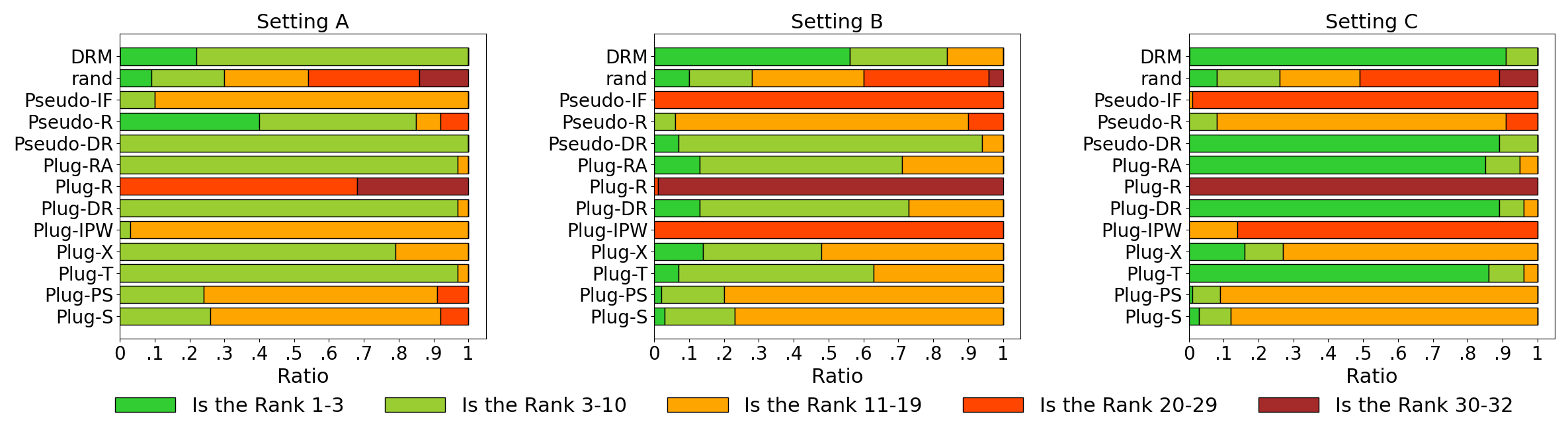
Figure 1: The stacked bar chart showing the distribution of the selected estimator’s rank for each evaluation metric across rank intervals: [1-3], [3-10], [11-19], [20-29], and [30-32]. The greener (or redder) color indicates that the selected estimator ranks higher (or lower). For example, the dark red (or green) indicates the percentage of cases (out of 100 experiments) where the selected estimator ranks among the worst 3 estimators, specifically as ranks 30, 31, or 32. (or among the best 3 estimators, specifically as ranks 1, 2, or 3).

5.2 Experimental Results

Part I: PEHE comparison.

The CATE estimator $\hat{\tau}$ is believed better if it achieves smaller $\mathcal{R}^{oracle}(\hat{\tau})$. Simultaneously, a better CATE estimator $\hat{\tau}$ also implies a smaller difference between $\mathcal{R}^{oracle}(\hat{\tau})$ and $\mathcal{R}^{oracle}(\hat{\tau}_{best})$, where $\hat{\tau}_{best}$ is the actual best estimator defined before equation (1). Consequently, we propose the following two criteria to compare estimators chosen by different selectors:

$$\sqrt{\text{PEHE}} =\mathcal{R}^{oracle}(\hat{\tau}_{select}),$$

Regret $$=\frac{\mathcal{R}^{oracle}(\hat{\tau}_{select})-\mathcal{R}^{oracle}(\hat{\tau}_{best})}{\mathcal{R}^{oracle}(\hat{\tau}_{best})}.$$

As evidenced by results regarding $\sqrt{\text{PEHE}}$ and Regret in Table 1, our proposed DRM method demonstrates effective and stable performance. Notably, in both settings B and C, DRM outperforms all other selectors, achieving the smallest $\sqrt{\text{PEHE}}$ and Regret values. Specifically, in setting B, DRM-selected estimators exhibit significantly lower average Regret compared to other selectors, while in setting C, the average $\sqrt{\text{PEHE}}$ of DRM-selected estimators closely matches that of the oracle estimator. Although pseudo-R performs better than DRM in setting A, it does not demonstrate the overall stability exhibited by DRM in settings B and C. It is worth mentioning that pseudo-DR, plug-DR, and plug-RA also show commendable performance.

Part II: Robustness examination.

Now we analyze the capability of each selector in capturing robustness from the following two aspects: (i) the ability to consistently select superior estimators; and (ii) the ability to mitigate the risk of selecting inferior estimators. In each of the 100 experiments, we sort all 32 estimators in ascending order based on their $\mathcal{R}^{oracle}(\hat{\tau})$ values, yielding a sorted list $[\mathcal{R}^{oracle}(\hat{\tau}_{1}),\dots,\mathcal{R}^{oracle}(\hat{\tau}_{J})]$. We then determine the actual rank of the selected estimator based on this list for each of the 100 experiments and plot the distribution of these 100 ranks in a stacked bar chart (Figure 1). The following observations highlight the significance of robustness in CATE estimator selection.

Firstly, our DRM excels not only in identifying the best estimators but also in mitigating the risk of selecting poor ones. Overall, DRM consistently outperforms other selectors in choosing the top 3 estimators across all settings. Although it may have a slight disadvantage compared to pseudo-R in setting A, none of the estimators selected by DRM perform worse than rank 10. Similar observations can be made in setting C. In setting B, while there are instances where DRM selects estimators ranked within 11-19, it still surpasses other metrics in selecting the top 3 estimators.

Secondly, when the ceiling performances of different selectors are comparable, the worst-case performance becomes a dominant factor. In setting C, pseudo-DR, plug-RA, plug-DR, and DRM exhibit similarly strong performances in selecting the top 3 estimators. However, pseudo-DR and DRM outperform the other two metrics in terms of $\sqrt{\text{PEHE}}$ and Regret, as all of their selected estimators are ranked within the top 10.

Thirdly, the consistency of good performances depends on robustness. In setting A, the pseudo-R selector often succeeds in choosing the top 3 estimators, resulting in lower values of $\sqrt{\text{PEHE}}$ and Regret. However, it fails to maintain consistently excellent performance in settings B and C. In contrast, our DRM consistently demonstrates superiority in various aspects in settings B and C, including $\sqrt{\text{PEHE}}$, Regret, and the ability to select the best estimators.

Part III: Ranking ability.

To assess the ranking ability of each evaluation metric, we calculate the Rank Correlation using Spearman rank correlation between the rank order determined by the oracle metric $\mathcal{R}^{oracle}(\hat{\tau})$ and the rank order determined by each evaluation metric (e.g., $\mathcal{R}^{plug}_{\tilde{\tau}}(\hat{\tau})$, $\mathcal{R}^{pseudo}_{\tilde{Y}}(\hat{\tau})$, and $\mathcal{R}^{DRM}(\hat{\tau})$). In Table 1, our DRM method consistently exhibits good performance in ranking estimators, outperforming other metrics in setting A while remaining comparable in settings B and C. However, DRM is relatively inferior to pseudo-DR, which achieves the best performance in ranking estimators across all settings. This disparity may stem from DRM selecting estimators based on their worst-case performance. While worst-case performance can serve as a good benchmark for selecting players to attend Olympics, it might not be a reasonable standard to rank players’ overall performance. This is because ranking inherently involves the concept of expected (average) performance, which is determined by neither the best nor the worst performance alone. It would be intriguing to explore methods that can enhance the ranking ability of our DRM approach in future research.

We also conduct similar comparisons of selected estimators among the total of 8 candidate estimators, with the underlying ML model fixed as LR, SVM, RF, or NN. The relevant results are reported in Appendix C for further reference.

6 Conclusion

This paper sheds light on the potential of robustness in selecting CATE estimators. We propose a novel evaluation method called the distributionally robust metric (DRM), which offers several advantages over existing metrics. Notably, our approach is model-free, eliminating the need for estimating nuisance parameters or plug-in learners. Moreover, it is specifically designed to select a robust CATE estimator, rather than pursue a “stellar” one, which is practically meaningful. We also provide a finite sample analysis that demonstrates a decay rate of $n^{-1/2}$ for the gap between $\hat{\mathcal{V}}(\hat{\tau})$ and $\mathcal{V}(\hat{\tau})$. The experimental results confirm the efficacy of our DRM approach in CATE estimator selection.

Limitations. We must acknowledge the DRM method is not a one-size-fits-all solution and still faces several challenges that require further research and attention. For example, exploring alternative approaches to derive a tighter PEHE bound and enhancing the ranking ability of DRM can be a promising avenue for future investigation. Moreover, inspired by the robust optimization literature (Hu & Hong, 2013; Mohajerin Esfahani & Kuhn, 2018; Kuhn et al., 2019; Levy et al., 2020; Wang et al., 2021), considering divergences other than KL for DRM would be an interesting next step. While our DRM method reveals the potential of robustness in selecting CATE estimators, it is important to note that the purpose of this paper is not to claim that we have discovered a silver bullet for CATE estimator selection. Our main intent is to provide valuable insights for practical decision-makers and stimulate increasing attention toward the topic of model selection in causal inference.

Appendix A CATE Estimation Strategies

A.1 CATE Learners

We now detail how to construct CATE learners using the observed samples $\{(X_{i},T_{i},Y_{i})\}_{i=1}^{n}$. Note that CATE learners are learned on the training set, so the sample size $n$ here equals the training sample size. Denote $n_{t}$ by the sample size in the treat group, and $n_{c}$ by the sample size in the control group such that $n=n_{t}+n_{c}$.

• S-learner: Let predictors=$(X,T)$, response=$Y$. Train a model $\hat{\mu}(X,T)$. Then we obtain $\hat{\tau}_{S}(X)$:

  $$\hat{\tau}_{S}(X)=\hat{\mu}(X,1)-\hat{\mu}(X,0).$$

• T-learner: Let predictors=$X^{T}$ (covariates in the treat), response=$Y^{T}$ (outcome in the treat). Train a model $\hat{\mu}_{1}(X)$. Let predictors=$X^{C}$ (covariates in the control), response=$Y^{C}$ (outcome in the control). Train a model $\hat{\mu}_{0}(X)$. Then we obtain $\hat{\tau}_{T}(X)$:

  $$\hat{\tau}_{T}(X)=\hat{\mu}_{1}(X)-\hat{\mu}_{0}(X).$$

• PS-learner: Fisrt-step: Train $\hat{\tau}_{S}(X)$ using the above-mentioned step in S-learner. Second-step: Let predictors=$X$, response=$\hat{\tau}_{S}(X)$. Train a model $\hat{\tau}_{PS}(X)$ from the following objective:

  $$\hat{\tau}_{PS}=\mathop{\arg\min}_{\tau}\;\frac{1}{n}\sum_{i=1}^{n}(\tau(X_{i})-\hat{\tau}_{S}(X_{i}))^{2}.$$

• IPW-learner: First-step: let predictors=$X$, response=$T$. Train a propensity score model $\hat{\pi}(X)$. Construct surrogate of CATE using pseudo-outcomes with inverse propensity weighting (IPW) formula: $Y_{IPW}^{1,0}=Y_{IPW}^{1}-Y_{IPW}^{0}$, where $Y_{IPW}^{1}=\frac{TY}{\hat{\pi}(X)}$ and $Y_{IPW}^{0}=\frac{(1-T)Y}{1-\hat{\pi}(X)}$. Train a model $\hat{\tau}_{IPW}(X)$ from the following objective:

  $$\hat{\tau}_{IPW}=\mathop{\arg\min}_{\tau}\;\frac{1}{n}\sum_{i=1}^{n}(\tau(X_{i})-Y_{i,IPW}^{1,0})^{2}.$$

• X-learner (Künzel et al., 2019): First-step: Train $\hat{\mu}_{1}(X)$ and $\hat{\mu}_{0}(X)$ using the the above-mentioned procedure in T-learner. Train a propensity score model $\hat{\pi}(X)$ using the the above-mentioned procedure in IPW-learner. Second-step: Let predictors=$X^{T}$, response=$\hat{\mu}_{1}(X^{T})-Y^{T}$, and predictors=$X^{C}$, response=$\hat{\mu}_{0}(X^{C})-Y^{C}$. Obtain a model $\hat{\tau}_{X}(X)$ by learning two separate functions $\hat{\tau}^{1}_{X}(X)$ and $\hat{\tau}^{0}_{X}(X)$:

  $$\hat{\tau}_{X}(X)=(1-\hat{\pi}(X))\hat{\tau}^{1}_{X}(X)+\hat{\pi}(X)\hat{\tau}^{0}_{X}(X),$$

  $$\hat{\tau}^{1}_{X}=\mathop{\arg\min}_{\tau}\;\frac{1}{n_{t}}\sum_{i=1}^{n_{t}}(\tau(X_{i})-(Y_{i}-\hat{\mu}_{0}(X_{i})))^{2},$$

  $$\hat{\tau}^{0}_{X}=\mathop{\arg\min}_{\tau}\;\frac{1}{n_{c}}\sum_{i=1}^{n_{c}}(\tau(X_{i})-(\hat{\mu}_{1}(X_{i})-Y_{i}))^{2}.$$

• DR-learner (Kennedy, 2023; Foster & Syrgkanis, 2023): First-step: Train $\hat{\mu}_{1}(X)$ and $\hat{\mu}_{0}(X)$ using the the above-mentioned procedure in T-learner. Train a propensity score model $\hat{\pi}(X)$ using the the above-mentioned procedure in IPW-learner. Second-step: Construct surrogate of CATE using pseudo-outcomes with doubly robust (DR) formula: $Y_{DR}^{1,0}=Y_{DR}^{1}-Y_{DR}^{0}$, where $Y_{DR}^{1}=\hat{\mu}_{1}(X)+\frac{T}{\hat{\pi}(X)}(Y-\hat{\mu}_{1}(X))$ and $Y_{DR}^{0}=\hat{\mu}_{0}(X)+\frac{1-T}{1-\hat{\pi}(X)}(Y-\hat{\mu}_{0}(X))$. Train a model $\hat{\tau}_{DR}(X)$ from the following objective:

  $$\hat{\tau}_{DR}=\mathop{\arg\min}_{\tau}\;\frac{1}{n}\sum_{i=1}^{n}(\tau(X_{i})-Y_{i,DR}^{1,0})^{2}.$$

• R-learner (Nie & Wager, 2021): First-step: Let predictors=$X$, response=$Y$. Train a model $\hat{\mu}(X)$ to approximate the conditional mean outcome $\mathbb{E}[Y|X]$. Train a propensity score model $\hat{\pi}(X)$ using the the above-mentioned procedure in IPW-learner. Second-step: Compute the outcome residual $\xi=Y-\hat{\mu}(X)$ and treatment residual $\nu=T-\hat{\pi}(X)$. Train a model $\hat{\tau}_{R}(X)$ from the following objective:

  $$\hat{\tau}_{R}=\mathop{\arg\min}_{\tau}\;\frac{1}{n}\sum_{i=1}^{n}(\xi_{i}-\nu_{i}\tau(X_{i}))^{2}.$$

• RA-learner (Curth & van der Schaar, 2021b): First-step: Train $\hat{\mu}_{1}(X)$ and $\hat{\mu}_{0}(X)$ using the the above-mentioned procedure in T-learner. Second-step: Construct surrogate of CATE using pseudo-outcomes with regression adjustment (RA) formula: $Y_{RA}=T(Y-\hat{\mu}_{0}(X))+(1-T)(\hat{\mu}_{1}(X)-Y)$. Train a model $\hat{\tau}_{RA}(X)$ from the following objective:

  $$\hat{\tau}_{RA}=\mathop{\arg\min}_{\tau}\;\frac{1}{n}\sum_{i=1}^{n}(\tau(X_{i})-Y_{i,RA})^{2}.$$

A.2 CATE Selectors

We now detail how to construct CATE selectors using the observed samples $\{(X_{i},T_{i},Y_{i})\}_{i=1}^{n}$. Note that CATE selectors are constructed on the validation set, so the sample size $n$ here equals the validation sample size.

• Plug-in selector: Obtain any CATE learners $\tilde{\tau}$ using the observational validation data. Then plug-in $\tilde{\tau}$ into the following metric $\mathcal{R}_{\tilde{\tau}}^{plug}(\hat{\tau})$:

  $$\mathcal{R}_{\tilde{\tau}}^{plug}(\hat{\tau})=\sqrt{\frac{1}{n}\sum_{i=1}^{n}(\hat{\tau}(X_{i})-\tilde{\tau}(X_{i}))^{2}}.$$

  For each plug-in selector $\tilde{\tau}$, the selected $j^{*}$-th CATE estimator is $\hat{\tau}_{j^{*}}$, where $j^{*}=\mathop{\arg\min}_{j\in\{1,\dots,J\}}\mathcal{R}_{\tilde{\tau}}^{plug}(\hat{\tau}_{j})$.

• Pseudo-outcome selector:

  1. Pseudo-DR: Utilize validation data to estimate nuisance parameters $(\tilde{\mu}_{1},\tilde{\mu}_{0},\tilde{\pi})$, following the procedure described in Section A.1. $\tilde{Y}_{DR}=\tilde{Y}_{DR}^{1}-\tilde{Y}_{DR}^{0}$, where $\tilde{Y}_{DR}^{1}=\tilde{\mu}_{1}(X)+\frac{T}{\tilde{\pi}(X)}(Y-\tilde{\mu}_{1}(X))$ and $\tilde{Y}_{DR}^{0}=\tilde{\mu}_{0}(X)+\frac{1-T}{1-\tilde{\pi}(X)}(Y-\tilde{\mu}_{0}(X))$. Then the pseudo-DR metric is

     $$\mathcal{R}_{DR}^{pseudo}(\hat{\tau})=\sqrt{\frac{1}{n}\sum_{i=1}^{n}(\hat{\tau}(X_{i})-\tilde{Y}_{i,DR})^{2}}.$$

     For pseudo-DR selector, the selected $j^{*}$-th CATE estimator is $\hat{\tau}_{j^{*}}$, where $j^{*}=\mathop{\arg\min}_{j\in\{1,\dots,J\}}\mathcal{R}_{DR}^{pseudo}(\hat{\tau}_{j})$.

  2. Pseudo-R: Utilize validation data to estimate nuisance parameters $(\tilde{\mu},\tilde{\pi})$, following the procedure described in Section A.1. Then the pseudo-R metric is

     $$\mathcal{R}_{R}^{pseudo}(\hat{\tau})=\sqrt{\frac{1}{n}\sum_{i=1}^{n}((Y_{i}-\tilde{\mu}(X_{i}))-\hat{\tau}(X_{i})(T_{i}-\tilde{\pi}(X_{i})))^{2}}.$$

     For pseudo-R selector, the selected $j^{*}$-th CATE estimator is $\hat{\tau}_{j^{*}}$, where $j^{*}=\mathop{\arg\min}_{j\in\{1,\dots,J\}}\mathcal{R}_{R}^{pseudo}(\hat{\tau}_{j})$.

  3. Pseudo-IF (Alaa & Van Der Schaar, 2019): Utilize validation data to estimate nuisance parameters $(\tilde{\mu}_{1},\tilde{\mu}_{0},\tilde{\pi})$, following the procedure described in Section A.1. Let $\tilde{\tau}(X)=(\tilde{\mu}_{1}(X)-\tilde{\mu}_{0}(X))$. Then the pseudo-IF metric is

     $$\mathcal{R}_{IF}^{pseudo}(\hat{\tau})=\sqrt{\frac{1}{n}\sum_{i=1}^{n}(1-B_{i})\tilde{\tau}^{2}(X_{i})+B_{i}Y_{i}(\tilde{\tau}(X_{i})-\hat{\tau}(X_{i}))-A_{i}(\tilde{\tau}(X_{i})-\hat{\tau}(X_{i}))^{2}+\hat{\tau}^{2}(X_{i})},$$

     $$where\ A_{i}=T_{i}-\tilde{\pi}(X_{i}),\ B_{i}=2T_{i}(T_{i}-\tilde{\pi}(X_{i}))C_{i}^{-1},\ C_{i}=\tilde{\pi}(X_{i})(1-\tilde{\pi}(X_{i})).$$

     For pseudo-IF selector, the selected $j^{*}$-th CATE estimator is $\hat{\tau}_{j^{*}}$, where $j^{*}=\mathop{\arg\min}_{j\in\{1,\dots,J\}}\mathcal{R}_{IF}^{pseudo}(\hat{\tau}_{j})$.

  4. Other pseudo-outcome selector: By manipulating the formula of $\tilde{Y}$, it is possible to create additional pseudo-outcome selectors, such as the pseudo-IPW selector. In our paper, we choose pseudo-DR as the baseline because it is representative in the causal inference literature and it often demonstrates superior performance, owing to its doubly robust property.

A.3 Supplementary for the PEHE Upper Bound of Representation Balancing Methods

Let $\Phi:\mathcal{X}\to\mathcal{R}$ denote the representation function, $h:\mathcal{R}\times\{0,1\}\rightarrow\mathcal{Y}$ denote the outcome function such that $h(\Phi(X),t)$ estimates $Y^{t}$ for $t\in\{0,1\}$, $Dist(P^{T}_{\Phi},P^{C}_{\Phi})$ denote the distributional distance (e.g., MMD distance) between treat and control representations, and CATE is estimated by $\hat{\tau}(X)=h(\Phi(X),1)-h(\Phi(X),0)$. According to (Shalit et al., 2017; Johansson et al., 2022), the PEHE w.r.t. $(h,\Phi)$ can be upper bounded as follows:

$$\epsilon_{PEHE}(h,\Phi)\leq 2\big{(}\epsilon_{F}^{T=1}(h,\Phi)+\epsilon_{F}^{T=0}(h,\Phi)+B_{\Phi}\cdot Dist(P^{T}_{\Phi},P^{C}_{\Phi})-2\sigma^{2}_{Y}\big{)}.$$ (18)

Here, $\epsilon_{PEHE}(h,\Phi)=\mathbb{E}[(h(\Phi(X),1)-h(\Phi(X),0)-\tau_{true}(X))^{2}]$ is the same as $\mathcal{R}(h(\Phi(\cdot),1)-h(\Phi(\cdot),0))$ in equation (1). $\epsilon_{F}^{T=t}(h,\Phi)=\mathbb{E}[(h(\Phi(X),t)-Y)^{2}|T=t]$ denotes the factual outcome estimation error in the treat ($t=1$) or control ($t=0$) group. $Dist(P^{T}_{\Phi},P^{C}_{\Phi})$ denotes the distributional distance (e.g., MMD distance) between treat and control groups in the representation space. $B_{\Phi}\geq 0$ is a constant such that for $t\in\{0,1\}$, the function $g_{\Phi,h}(r,t):=\frac{1}{B_{\Phi}}\cdot\ell_{h,\Phi}(\Psi(r),t)\in\mathcal{G}$, where $\Psi$ is the inverse of $\Phi$ and $\mathcal{G}$ is the family of 1-Lipschitz functions. $\sigma_{y}^{2}$ is a constant such that $\sigma_{y}^{2}=\min\{\sigma^{2}_{y^{t}}(p(x,t)),\sigma^{2}_{y^{t}}(p(x,1-t))\}$, where $\sigma^{2}_{y^{t}}(p(x,t))=\int_{\mathcal{X}\times\{0,1\}\times\mathcal{Y}}(y^{t}-\tau^{t}(x))^{2}p(y^{t}|x)p(x,t)dy^{t}dxdt$. This bound offers a guiding principle for representation balancing methods mentioned in Section 2: Due to the unavailability of the true PEHE $\epsilon_{PEHE}(h,\Phi)$, the objective function of a representation balancing model should aim to minimize the PEHE upper bound that involves the error in factual outcomes and the distributional distance between the treat and control representations.

Appendix B Proofs

B.1 Proof of Proposition 4.1

Proof.

$$\mathbb{E}[(\hat{\tau}(X)-\tau_{true}(X))^{2}]$$

$$=\mathbb{E}[(\hat{\tau}(X)-(\mu_{1}(X)-\mu_{0}(X)))^{2}]$$

$$=\mathbb{E}[(\hat{\tau}(X)-\mu_{1}(X)+\mu_{0}(X))^{2}]$$

$$\leq 2\left[\mathbb{E}[(\hat{\tau}(X)-\mu_{1}(X))^{2}]+\mathbb{E}[(\mu_{0}(X))^{2}]\right]$$

$$=2\left[\mathbb{E}[(\hat{\tau}(X)-Y^{1}+Y^{1}-\mu_{1}(X))^{2}]+\mathbb{E}[(\mu_{0}(X))^{2}]\right]$$

$$=2\left[\mathbb{E}[(\hat{\tau}(X)-Y^{1})^{2}]+\mathbb{E}[(Y^{1}-\mu_{1}(X))^{2}]+2\mathbb{E}[(\hat{\tau}(X)-Y^{1})(Y^{1}-\mu_{1}(X))]+\mathbb{E}[(\mu_{0}(X))^{2}]\right]$$

$$=2\left[\mathbb{E}[(\hat{\tau}(X)-Y^{1})^{2}]+\mathbb{E}[(Y^{1}-\mu_{1}(X))^{2}]+2\mathbb{E}[\hat{\tau}(X)Y^{1}-\hat{\tau}(X)\mu_{1}(X)-(Y^{1})^{2}+Y^{1}\mu_{1}(X)]+\mathbb{E}[(\mu_{0}(X))^{2}]\right]$$

$$=2\left[\mathbb{E}[(\hat{\tau}(X)-Y^{1})^{2}]+\mathbb{E}[(Y^{1}-\mu_{1}(X))^{2}]+2\mathbb{E}[\mathbb{E}[\hat{\tau}(X)Y^{1}-\hat{\tau}(X)\mu_{1}(X)-(Y^{1})^{2}+Y^{1}\mu_{1}(X)|X]]+\mathbb{E}[(\mu_{0}(X))^{2}]\right]$$

$$=2\left[\mathbb{E}[(\hat{\tau}(X)-Y^{1})^{2}]+\mathbb{E}[(Y^{1}-\mu_{1}(X))^{2}]+2\mathbb{E}[\hat{\tau}(X)\mathbb{E}[Y^{1}|X]-\hat{\tau}(X)\mu_{1}(X)-\mathbb{E}[(Y^{1})^{2}|X]+\mathbb{E}[Y^{1}|X]\mu_{1}(X)]+\mathbb{E}[(\mu_{0}(X))^{2}]\right]$$

$$=2\left[\mathbb{E}[(\hat{\tau}(X)-Y^{1})^{2}]+\mathbb{E}[(Y^{1}-\mu_{1}(X))^{2}]+2\mathbb{E}[\hat{\tau}(X)\mu_{1}(X)-\hat{\tau}(X)\mu_{1}(X)-\mathbb{E}[(Y^{1})^{2}|X]+\mu_{1}(X)\mu_{1}(X)]+\mathbb{E}[(\mu_{0}(X))^{2}]\right]$$

$$=2\left[\mathbb{E}[(\hat{\tau}(X)-Y^{1})^{2}]+\mathbb{E}[(Y^{1}-\mu_{1}(X))^{2}]+2\mathbb{E}[(\mu_{1}(X))^{2}]-2\mathbb{E}[(Y^{1})^{2}]+\mathbb{E}[(\mu_{0}(X))^{2}]\right]$$

$$=2\left[\mathbb{E}[(\hat{\tau}(X)-Y^{1})^{2}]+\mathbb{E}[(Y^{1})^{2}]+\mathbb{E}[(\mu_{1}(X))^{2}]-2\mathbb{E}[Y^{1}\mu_{1}(X)]+2\mathbb{E}[(\mu_{1}(X))^{2}]-2\mathbb{E}[(Y^{1})^{2}]+\mathbb{E}[(\mu_{0}(X))^{2}]\right]$$

$$=2\left[\mathbb{E}[(\hat{\tau}(X)-Y^{1})^{2}]+\mathbb{E}[(Y^{1})^{2}]+\mathbb{E}[(\mu_{1}(X))^{2}]-2\mathbb{E}[\mu_{1}(X)\mathbb{E}[Y^{1}|X]]+2\mathbb{E}[(\mu_{1}(X))^{2}]-2\mathbb{E}[(Y^{1})^{2}]+\mathbb{E}[(\mu_{0}(X))^{2}]\right]$$

$$=2\left[\mathbb{E}[(\hat{\tau}(X)-Y^{1})^{2}]+\mathbb{E}[(\mu_{1}(X))^{2}]-\mathbb{E}[(Y^{1})^{2}]+\mathbb{E}[(\mu_{0}(X))^{2}]\right]$$

$$=2\left[\mathbb{E}[(\hat{\tau}(X)-Y^{1})^{2}]+\mathbb{V}[\mu_{1}(X)]+(\mathbb{E}[\mu_{1}(X)])^{2}-\mathbb{V}[Y^{1}]-(\mathbb{E}[Y^{1}])^{2}+\mathbb{V}[\mu_{0}(X)]+(\mathbb{E}[\mu_{0}(X)])^{2}\right]$$

$$=2\left[\mathbb{E}[(\hat{\tau}(X)-Y^{1})^{2}]+\mathbb{V}[\mu_{1}(X)]-\mathbb{V}[Y^{1}]+\mathbb{V}[\mu_{0}(X)]+(\mathbb{E}[\mu_{0}(X)])^{2}\right]$$

$$=2\left[\mathbb{E}[(\hat{\tau}(X)-Y^{1})^{2}]+\zeta\right].$$

∎

B.2 Proof of Proposition 4.6

We first propose the following Proposition that is useful in proving Proposition 4.6.

Proposition B.1.

Assume the random variable tuple $(X,T,Y^{1},Y^{0})$ satisfies Assumption 3.1. For any $t\in\{0,1\}$, we have

$$P(X,Y^{1}|T=t)=P(Y^{1}|X)P(X|T=t).$$ (19)

Proof.

$$P(X,Y^{1}|T=t)$$

$$= P(Y^{1}|X,T=t)P(X|T=t)$$

$$= P(Y^{1}|X)P(X|T=t).\quad\text{(Unconfoundedness)}$$

∎

Now we can prove Proposition 4.6.

Proof.

$$D_{KL}(P(X,Y^{1}|T=0)||P(X,Y^{1}|T=1))$$

$$= \int_{\mathcal{X}}\int_{\mathcal{Y}^{1}}p(x,y^{1}|T=0)\log\frac{p(x,y^{1}|T=0)}{p(x,y^{1}|T=1)}dy^{1}dx$$

$$= \int_{\mathcal{X}}\int_{\mathcal{Y}^{1}}p(y^{1}|x)p(x|T=0)\log\frac{p(y^{1}|x)p(x|T=0)}{p(y^{1}|x)p(x|T=1)}dy^{1}dx\quad\text{(By Proposition \ref{prop:prob_decompose})}$$

$$= \int_{\mathcal{X}}\int_{\mathcal{Y}^{1}}p(y^{1}|x)p(x|T=0)\log\frac{p(x|T=0)}{p(x|T=1)}dy^{1}dx$$

$$= \int_{\mathcal{X}}\left(\int_{\mathcal{Y}^{1}}p(y^{1}|x)dy^{1}\right)p(x|T=0)\log\frac{p(x|T=0)}{p(x|T=1)}dx$$

$$= \int_{\mathcal{X}}p(x|T=0)\log\frac{p(x|T=0)}{p(x|T=1)}dx$$

$$= D_{KL}(P(X|T=0)||P(X|T=1)).$$

∎

B.3 Proof of Theorem 4.4

We first recall the results in (Hu & Hong, 2013).

Lemma B.2 (Theorem 1 in (Hu & Hong, 2013)).

Let $f_{\theta}(x)$ denote the loss function of $x$ and it is bounded almost surely. $\theta\in\Theta$ represents the model parameters of the function $f_{\theta}(x)$. Let $\mathcal{B}_{\epsilon}(P)$ be the uncertainty ball centered at distribution $P$ with ambiguity radius $\epsilon$. Define $\kappa$ as the mass of the distribution $P$ on its essential supremum (Proposition 2 in (Hu & Hong, 2013)). Assume $f_{\theta}(x)$ is bounded and $\log\kappa+\epsilon<0$, then we have

$$\mathcal{V}:=\sup_{Q\in\mathcal{B}_{\epsilon}(P)}\mathbb{E}^{Q}[f_{\theta}(x)]=\min_{\lambda>0}\lambda\epsilon+\lambda\log\mathbb{E}^{P}[\exp(f_{\theta}(x)/\lambda)].$$

Our Theorem 4.4 follows by directly applying the above Lemma B.2.

B.4 Proof of Theorem 4.5

For notational simplicity, we denote $Z=(\hat{\tau}(X)-Y)^{2}$, $W=(Z,T)\in\mathcal{W}$, and $g(\lambda;W)=T\exp\left(Z/\lambda\right)$. Then, we define the following two functions:

$$G(\lambda;W)=\mathbb{E}[g(\lambda;W)];$$ (20)

$$\hat{G}(\lambda;W)=\frac{1}{n}\sum_{i=1}^{n}g(\lambda;W_{i}).$$ (21)

Then we have the following lemma that guarantees the convergence for $\hat{G}(\lambda;W)$.

Lemma B.3.

Assuming that $0<\underaccent{\bar}{\lambda}\leq\lambda\leq\bar{\lambda}$ and $(\hat{\tau}(X)-Y)^{2}$ is upper bounded by $\bar{M}$. Then with probability $1-\delta$, we have

$$|\hat{G}(\lambda;W)-G(\lambda;W)|\leq\mathcal{O}\left(\sqrt{\frac{2\log\frac{2}{\delta}\left(\exp\left(\bar{M}/\underaccent{\bar}{\lambda}\right)\right)^{2}}{n}}\right).$$

Proof.

Denote $h(W_{1},W_{2},\dots,W_{n})=\frac{1}{n}\sum_{i=1}^{n}g(\lambda;W_{i})$. First, we notice that $h(W_{1},W_{2},\dots,W_{n})$ satisfies the bounded difference inequality:

$$\sup_{W_{1},\dots,W_{n},W_{i}^{\prime}\in\mathcal{W}}\left|h(W_{1},\dots,W_{i},\cdots,W_{n})-h(W_{1},\dots,W_{i}^{\prime},\cdots,W_{n})\right|$$ (22)

$$=\sup_{W_{i},W_{i}^{\prime}\in\mathcal{W}}\frac{\left|g(\lambda;W_{i})-g(\lambda;W_{i}^{\prime})\right|}{n}$$

$$\leq 2\sup_{W_{i}\in\mathcal{W}}\frac{|g(\lambda;W_{i})|}{n}\leq\frac{2\exp\left(\bar{M}/\lambda\right)}{n}.$$

Note that $|\hat{G}(\lambda;W)-G(\lambda;W)|=|h(W_{1},W_{2},\dots,W_{n})-\mathbb{E}[h(W_{1},W_{2},\dots,W_{n})]|$. Then using McDiarmid’s inequality, for any $\epsilon>0$, we have

$$P\left(\left|\hat{G}(\lambda;W)-G(\lambda;W)\right|\geq\epsilon\right)$$ (23)

$$=P\left(\left|h(W_{1},W_{2},\dots,W_{n})-\mathbb{E}[h(W_{1},W_{2},\dots,W_{n})]\right|\geq\epsilon\right)$$

$$\leq 2\exp\left(-\frac{2\epsilon^{2}}{n(\frac{2\exp\left(\bar{M}/\lambda\right)}{n})^{2}}\right)=2\exp\left(\frac{-n\epsilon^{2}}{2\left(\exp\left(\bar{M}/\lambda\right)\right)^{2}}\right).$$

For some $\delta>0$, we have

$$P\left(\left|\hat{G}(\lambda;W)-G(\lambda;W)\right|\geq\epsilon\right)\leq 2\exp\left(\frac{-n\epsilon^{2}}{2\left(\exp\left(\bar{M}/\lambda\right)\right)^{2}}\right)\leq 2\exp\left(\frac{-n\epsilon^{2}}{2\left(\exp\left(\bar{M}/\underaccent{\bar}{\lambda}\right)\right)^{2}}\right)\leq\delta.$$ (24)

This solves $\epsilon$ such that

$$\epsilon\geq\sqrt{\frac{2\log\frac{2}{\delta}\left(\exp\left(\bar{M}/\underaccent{\bar}{\lambda}\right)\right)^{2}}{n}}.$$ (25)

∎

In the following content, we will bound the term $\left|\log(\hat{G}(\lambda;W))-\log\left(G(\lambda;W)\right)\right|$. We first introduce Lemma B.4 that is useful for bounding $\left|\log(\hat{G}(\lambda;W))-\log\left(G(\lambda;W)\right)\right|$.

Lemma B.4.

Let $c$ be a constant. For any $x_{1}$, $x_{2}$ such that $x_{1},x_{2}\geq c>0$, we have $|\log(x_{1})-\log(x_{2})|\leq\frac{1}{c}|x_{1}-x_{2}|$.

Proof.

Without loss of generality, assume $0<c\leq x_{1}\leq x_{2}$. We then have

$$\log(x_{2})-\log(x_{1})=\log(\frac{x_{2}}{x_{1}})=\log(1+\frac{x_{2}}{x_{1}}-1)\leq\frac{x_{2}}{x_{1}}-1=\frac{x_{2}-x_{1}}{x_{1}}\leq\frac{x_{2}-x_{1}}{c}.$$

Taking the absolute value of both the left-hand side and the right-hand side, we have

$$|\log(x_{1})-\log(x_{2})|\leq\frac{1}{c}|x_{1}-x_{2}|.$$

∎

Next, we introduce Lemma B.5 that bounds the term $\left|\log(\hat{G}(\lambda;W))-\log\left(G(\lambda;W)\right)\right|$.

Lemma B.5.

Let $u$ denote the probability of treat, i.e., $u=P(T=1)$. Assuming that $\lambda\in\Lambda:=(0,\bar{\lambda}]$ and $(\hat{\tau}(X)-Y)^{2}$ is bounded below by $\underaccent{\bar}{M}$. Then for $n\geq\frac{2}{u^{2}}\log\left(\frac{2}{\delta}\right)$, with probability $1-\delta$, we have

$$\left|\log(\hat{G}(\lambda;W))-\log\left(G(\lambda;W)\right)\right|$$ (26)

$$=\left|\log(\frac{1}{n}\sum_{i=1}^{n}T_{i}\exp\left(Z_{i}/\lambda\right))-\log\left(\mathbb{E}\left[T\exp\left(Z/\lambda\right)\right]\right)\right|$$

$$\leq\frac{2}{u\exp\left(\underaccent{\bar}{M}/\bar{\lambda}\right)}\left|\frac{1}{n}\sum_{i=1}^{n}T_{i}\exp\left(Z_{i}/\lambda\right)-\mathbb{E}\left[T\exp\left(Z/\lambda\right)\right]\right|.$$

Proof.

As both $\hat{G}(\lambda;W)$ and $G(\lambda;W)$ are bounded below and greater than $0$. Therefore, by Lemma B.4, we have

$$\left|\log(\hat{G}(\lambda;W))-\log\left(G(\lambda;W)\right)\right|\leq\frac{1}{c}\left|\hat{G}(\lambda;W)-G(\lambda;W)\right|,$$ (27)

$$\text{where}\;c=\min\left\{\inf_{\lambda\in\Lambda,W\in\mathcal{W}}\hat{G}(\lambda;W),\ \inf_{\lambda\in\Lambda,W\in\mathcal{W}}G(\lambda;W)\right\}.$$

Moreover, for any $\lambda\in\Lambda$, we have

$$G(\lambda;W)=\mathbb{E}[T\exp(Z/\lambda)]=\mathbb{E}[\exp(Z/\lambda)]P(T=1)\geq\mathbb{E}[\exp(\underaccent{\bar}{M}/\bar{\lambda})]u=\exp(\underaccent{\bar}{M}/\bar{\lambda})u;$$ (28)

$$\hat{G}(\lambda;W)=\frac{1}{n}\sum_{i=1}^{n}T_{i}\exp(Z_{i}/\lambda)\geq\frac{1}{n}\sum_{i=1}^{n}T_{i}\exp(\underaccent{\bar}{M}/\bar{\lambda})=\exp(\underaccent{\bar}{M}/\bar{\lambda})\frac{1}{n}\sum_{i=1}^{n}T_{i}=\exp(\underaccent{\bar}{M}/\bar{\lambda})\hat{u}.$$ (29)

Given $\hat{u}=\frac{1}{n}\sum_{i=1}^{n}T_{i}$ and $u=\mathbb{E}[\frac{1}{n}\sum_{i=1}^{n}T_{i}]$, using Hoeffding’s inequality, we have

$$P\left(\left|\frac{1}{n}\sum_{i=1}^{n}T_{i}-\mathbb{E}[\frac{1}{n}\sum_{i=1}^{n}T_{i}]\right|\geq\frac{\mathbb{E}[\frac{1}{n}\sum_{i=1}^{n}T_{i}]}{2}\right)\leq 2\exp\left(-\frac{2(\frac{u}{2})^{2}}{n(\frac{1}{n})^{2}}\right)\leq\delta.$$ (30)

We can solve $n$ by

$$2\exp\left(-\frac{nu^{2}}{2}\right)\leq\delta\Rightarrow n\geq\frac{2}{u^{2}}\log\left(\frac{2}{\delta}\right).$$ (31)

This indicates that $\hat{u}\geq u/2$ with probability $1-\delta$ when $n\geq\frac{2}{u^{2}}\log\left(\frac{2}{\delta}\right)$. Combining this with equations (28) and (29), with probability $1-\delta$, when $n\geq\frac{2}{u^{2}}\log\left(\frac{2}{\delta}\right)$, we have

$$\inf_{\lambda\in\Lambda,W\in\mathcal{W}}G(\lambda;W)\geq\exp(\underaccent{\bar}{M}/\bar{\lambda})u;$$ (32)

$$\inf_{\lambda\in\Lambda,W\in\mathcal{W}}\hat{G}(\lambda;W)\geq\exp(\underaccent{\bar}{M}/\bar{\lambda})\hat{u}\geq\exp(\underaccent{\bar}{M}/\bar{\lambda})u/2.$$ (33)

Therefore, with probability $1-\delta$, when $n\geq\frac{2}{u^{2}}\log\left(\frac{2}{\delta}\right)$, we have

$$\left|\log(\hat{G}(\lambda;W))-\log\left(G(\lambda;W)\right)\right|\leq\frac{1}{c}\left|\hat{G}(\lambda;W)-G(\lambda;W)\right|,$$ (34)

$$\text{where}\;c=\min\left\{\inf_{W\in\mathcal{W}}\hat{G}(\lambda;W),\ \inf_{W\in\mathcal{W}}G(\lambda;W)\right\}=\exp(\underaccent{\bar}{M}/\bar{\lambda})u/2.$$

This completes the proof of Lemma B.5. ∎

Additionally, the following Lemma B.6 provides the bound of $|\log(\hat{u})-\log(u)|$.

Lemma B.6.

Let $\hat{u}=\frac{1}{n}\sum_{i=1}^{n}T_{i}$ and $u=\mathbb{E}[\frac{1}{n}\sum_{i=1}^{n}T_{i}]$. For $n\geq\frac{2}{u^{2}}\log\left(\frac{2}{\delta}\right)$, with probability $1-\delta$, we have

$$|\log(\hat{u})-\log(u)|\leq\mathcal{O}\left(\sqrt{\frac{2\log(\frac{2}{\delta})}{nu^{2}}}\right).$$ (35)

Proof.

Using Hoeffding’s inequality, we have

$$P(|\hat{u}-u|\geq\epsilon)=P\left(\left|\frac{1}{n}\sum_{i=1}^{n}T_{i}-\mathbb{E}[\frac{1}{n}\sum_{i=1}^{n}T_{i}]\right|\geq\epsilon\right)\leq 2\exp\left(-2n\epsilon^{2}\right),$$

$$2\exp\left(-2n\epsilon^{2}\right)\leq\delta\quad\text{solves}\quad\epsilon\geq\sqrt{\frac{\log(\frac{2}{\delta})}{2n}}.$$

Notably, using the results in equation (31), we know for $n\geq\frac{2}{u^{2}}\log\left(\frac{2}{\delta}\right)$, $\hat{u}\geq u/2$. Therefore, we have

$$|\log(\hat{u})-\log(u)| \leq\frac{1}{\min\{\hat{u},u\}}|\hat{u}-u|.\quad\text{(By Lemma \ref{lemma:log})}$$ (36)

$$=\frac{2}{u}|\hat{u}-u|\leq\frac{2}{u}\mathcal{O}\left(\sqrt{\frac{\log(\frac{2}{\delta})}{2n}}\right)=\mathcal{O}\left(\sqrt{\frac{2\log(\frac{2}{\delta})}{nu^{2}}}\right).$$

∎

In the following, we will bound the term $|\hat{\mathcal{V}}(\hat{\tau})-\mathcal{V}(\hat{\tau})|$ using above lemmas. We first define two functions $F(\lambda)$ and $\hat{F}(\lambda)$:

$$F(\lambda)=\lambda\epsilon+\lambda\log(\mathbb{E}^{P_{T}}[\exp((\hat{\tau}(X)-Y)^{2}/\lambda)])=\lambda\epsilon+\lambda\log\left(\frac{1}{u}\mathbb{E}[T\exp((\hat{\tau}(X)-Y)^{2}/\lambda)]\right);$$ (37)

$$\hat{F}(\lambda)=\lambda\epsilon+\lambda\log(\frac{1}{n_{t}}\sum_{i=1}^{n}T_{i}\exp((\hat{\tau}(X_{i})-Y_{i})^{2}/\lambda))=\lambda\epsilon+\lambda\log\left(\frac{1}{n\hat{u}}\sum_{i=1}^{n}T_{i}\exp((\hat{\tau}(X_{i})-Y_{i})^{2}/\lambda)\right).$$ (38)

The following Lemma B.7 bounds the term $|\hat{F}(\lambda)-F(\lambda)|$.

Lemma B.7.

Let $u:=P(T=1)$. Assuming that $0<\underaccent{\bar}{\lambda}\leq\lambda\leq\bar{\lambda}$ and $(\hat{\tau}(X)-Y)^{2}$ is bounded within the range of $\underaccent{\bar}{M}$ to $\bar{M}$, for $n\geq 2/u^{2}\log(2/\delta)$, with probability $1-\delta$, we have

$$|\hat{F}(\lambda)-F(\lambda)|\leq\mathcal{O}\left(\sqrt{\frac{8\lambda^{2}\log\frac{2}{\delta}}{nu^{2}}\left(\exp(\bar{M}/\underaccent{\bar}{\lambda}-\underaccent{\bar}{M}/\bar{\lambda}))\right)^{2}}\right)+\mathcal{O}\left(\sqrt{\frac{2\lambda^{2}\log(\frac{2}{\delta})}{nu^{2}}}\right).$$ (39)

Proof.

$$|\hat{F}(\lambda)-F(\lambda)|$$ (40)

$$=\left|\lambda\left(\log\left(\frac{1}{u}\mathbb{E}[T\exp((\hat{\tau}(X)-Y)^{2}/\lambda)]\right)-\log\left(\frac{1}{n\hat{u}}\sum_{i=1}^{n}T_{i}\exp((\hat{\tau}(X_{i})-Y_{i})^{2}/\lambda)\right)\right)\right|$$

$$=\lambda\left|\log\left(\mathbb{E}[T\exp((\hat{\tau}(X)-Y)^{2}/\lambda)]\right)-\log\left(\frac{1}{n}\sum_{i=1}^{n}T_{i}\exp((\hat{\tau}(X_{i})-Y_{i})^{2}/\lambda)\right)+\log(\hat{u})-\log(u)\right|$$

$$\leq\lambda\left|\log\left(\mathbb{E}[T\exp((\hat{\tau}(X)-Y)^{2}/\lambda)]\right)-\log\left(\frac{1}{n}\sum_{i=1}^{n}T_{i}\exp((\hat{\tau}(X_{i})-Y_{i})^{2}/\lambda)\right)\right|+\lambda\left|\log(\hat{u})-\log(u)\right|$$

$$\leq\frac{2\lambda}{u\exp(\underaccent{\bar}{M}/\bar{\lambda})}\left|\frac{1}{n}\sum_{i=1}^{n}T_{i}e^{\frac{(\hat{\tau}(X_{i})-Y_{i})^{2}}{\lambda}}-\mathbb{E}[Te^{\frac{(\hat{\tau}(X)-Y)^{2}}{\lambda}}]\right|+\lambda\left|\log(\hat{u})-\log(u)\right|\quad\text{(By Lemma \ref{lemma:bound for G})}$$

$$\leq\frac{2\lambda}{u\exp(\underaccent{\bar}{M}/\bar{\lambda})}\mathcal{O}\left(\sqrt{\frac{2\log\frac{2}{\delta}\left(\exp\left(\bar{M}/\underaccent{\bar}{\lambda}\right)\right)^{2}}{n}}\right)+\mathcal{O}\left(\sqrt{\frac{2\lambda^{2}\log(\frac{2}{\delta})}{nu^{2}}}\right)\quad\text{(By Lemma \ref{lemma:convergence of G} and Lemma \ref{lemma:log_u})}$$

$$=\mathcal{O}\left(\sqrt{\frac{8\lambda^{2}\log\frac{2}{\delta}}{nu^{2}}\left(\exp(\bar{M}/\underaccent{\bar}{\lambda}-\underaccent{\bar}{M}/\bar{\lambda})\right)^{2}}\right)+\mathcal{O}\left(\sqrt{\frac{2\lambda^{2}\log(\frac{2}{\delta})}{nu^{2}}}\right).$$

∎

Now, we can prove the result in Theorem 4.5.

Proof.

Let $\hat{\lambda}=\arg\min_{\lambda}\hat{F}(\lambda)$ and $\lambda^{*}=\arg\min_{\lambda}F(\lambda)$. Then we have

$$\mathcal{V}(\hat{\tau})-\hat{\mathcal{V}}(\hat{\tau}) =F(\lambda^{*})-\hat{F}(\hat{\lambda})$$ (41)

$$=F(\lambda^{*})-\hat{F}(\hat{\lambda})+F(\hat{\lambda})-F(\hat{\lambda})$$

$$=F(\hat{\lambda})-\hat{F}(\hat{\lambda})+F(\lambda^{*})-F(\hat{\lambda})$$

$$\leq|F(\hat{\lambda})-\hat{F}(\hat{\lambda})|+0$$

$$\leq\sup_{\lambda}|F(\lambda)-\hat{F}(\lambda)|.$$

$$\hat{\mathcal{V}}(\hat{\tau})-\mathcal{V}(\hat{\tau}) =\hat{F}(\hat{\lambda})-F(\lambda^{*})$$ (42)

$$=\hat{F}(\hat{\lambda})-F(\lambda^{*})+\hat{F}(\lambda^{*})-\hat{F}(\lambda^{*})$$

$$=\hat{F}(\lambda^{*})-F(\lambda^{*})+\hat{F}(\hat{\lambda})-\hat{F}(\lambda^{*})$$

$$\leq|\hat{F}(\lambda^{*})-F(\lambda^{*})|+0$$

$$\leq\sup_{\lambda}|\hat{F}(\lambda)-F(\lambda)|.$$

Based on the above two inequalities and taking the $\sup$ operation for both first and last terms of equation (40), we have

$$|\hat{\mathcal{V}}(\hat{\tau})-\mathcal{V}(\hat{\tau})| \leq\sup_{\lambda}|\hat{F}(\lambda)-F(\lambda)|$$ (43)

$$\leq\mathcal{O}\left(\sqrt{\frac{8\bar{\lambda}^{2}\log\frac{2}{\delta}}{nu^{2}}\left(\exp(\bar{M}/\underaccent{\bar}{\lambda}-\underaccent{\bar}{M}/\bar{\lambda})\right)^{2}}\right)+\mathcal{O}\left(\sqrt{\frac{2\bar{\lambda}^{2}\log(\frac{2}{\delta})}{nu^{2}}}\right).\quad\text{(By Lemma \ref{lemma:bound for F})}$$

∎

Appendix C Additional Experimental Results

Table 2: Comparison of different selectors across Settings A, B, and C. The estimator selection is over 8 candidate estimators, with underlying ML model fixed as LR. Reported values (mean $\pm$ standard deviation) are computed over 100 experiments. Bold denotes the best results among all selectors. $\sqrt{\text{PEHE}}$ & Regret: Smaller is better. Rank correlation: Larger is better.

Criterion	$\sqrt{\text{PEHE}}$ (with $\mathcal{R}(\hat{\tau}_{best})$ provided)			Regret			Rank Correlation
Setting	A (0.24$\pm$0.04)	B (15.49$\pm$1.84)	C (16.10$\pm$2.49)	A	B	C	A	B	C
Plug-S	29.07$\pm$5.36	27.92$\pm$5.28	35.11$\pm$6.72	122.99$\pm$32.59	0.80$\pm$0.25	1.20$\pm$0.37	-0.14$\pm$0.17	0.75$\pm$0.07	0.71$\pm$0.04
Plug-PS	29.35$\pm$5.39	28.41$\pm$5.13	36.00$\pm$5.98	124.20$\pm$32.87	0.83$\pm$0.23	1.26$\pm$0.32	-0.17$\pm$0.17	0.74$\pm$0.07	0.70$\pm$0.04
Plug-T	13.64$\pm$4.00	25.76$\pm$5.21	17.73$\pm$5.09	57.17$\pm$19.76	0.67$\pm$0.29	0.11$\pm$0.33	0.79$\pm$0.11	0.81$\pm$0.06	0.85$\pm$0.04
Plug-X	18.82$\pm$9.45	25.02$\pm$6.21	31.56$\pm$8.53	79.78$\pm$44.55	0.61$\pm$0.35	0.98$\pm$0.51	0.57$\pm$0.19	0.84$\pm$0.07	0.77$\pm$0.05
Plug-IPW	29.12$\pm$3.49	61.01$\pm$12.28	63.48$\pm$17.82	123.27$\pm$27.76	2.93$\pm$0.54	2.96$\pm$1.00	0.16$\pm$0.16	0.32$\pm$0.10	0.40$\pm$0.12
Plug-DR	13.63$\pm$4.32	23.72$\pm$5.58	17.36$\pm$5.25	57.02$\pm$20.43	0.54$\pm$0.32	0.08$\pm$0.30	0.79$\pm$0.11	0.85$\pm$0.07	0.85$\pm$0.04
Plug-R	37.89$\pm$5.12	159.18$\pm$21.16	164.11$\pm$21.59	160.73$\pm$37.79	9.27$\pm$0.52	9.30$\pm$1.23	-0.54$\pm$0.14	-0.46$\pm$0.08	-0.51$\pm$0.05
Plug-RA	13.72$\pm$4.24	23.97$\pm$5.52	17.91$\pm$5.67	57.40$\pm$20.27	0.55$\pm$0.33	0.12$\pm$0.36	0.79$\pm$0.11	0.84$\pm$0.06	0.85$\pm$0.04
Pseudo-DR	12.57$\pm$2.99	21.91$\pm$4.05	16.80$\pm$3.14	52.53$\pm$15.66	0.42$\pm$0.24	0.05$\pm$0.18	0.81$\pm$0.09	0.88$\pm$0.05	0.86$\pm$0.03
Pseudo-R	7.29$\pm$11.76	32.20$\pm$8.25	42.99$\pm$8.61	30.97$\pm$53.76	1.09$\pm$0.52	1.70$\pm$0.53	0.73$\pm$0.27	0.61$\pm$0.13	0.64$\pm$0.12
Pseudo-IF	28.72$\pm$3.77	84.44$\pm$14.30	82.31$\pm$12.27	121.69$\pm$28.65	4.45$\pm$0.64	4.17$\pm$0.72	0.32$\pm$0.15	0.33$\pm$0.09	0.41$\pm$0.09
Random	1780.99$\pm$7173.08	486.98$\pm$3141.69	2602.77$\pm$11333.92	7195.34$\pm$29304.08	39.39$\pm$266.19	170.40$\pm$738.22	-0.01$\pm$0.10	0.15$\pm$0.09	0.09$\pm$0.08
DRM	8.48$\pm$5.99	19.69$\pm$6.47	16.62$\pm$3.03	35.01$\pm$26.22	0.27$\pm$0.39	0.04$\pm$0.15	0.81$\pm$0.08	0.87$\pm$0.06	0.81$\pm$0.07

Table 3: Comparison of different selectors across Settings A, B, and C. The estimator selection is over 8 candidate estimators, with underlying ML model fixed as SVM. Reported values (mean $\pm$ standard deviation) are computed over 100 experiments. Bold denotes the best results among all selectors. $\sqrt{\text{PEHE}}$ & Regret: Smaller is better. Rank correlation: Larger is better.

Criterion	$\sqrt{\text{PEHE}}$ (with $\mathcal{R}(\hat{\tau}_{best})$ provided)			Regret			Rank Correlation
Setting	A (15.22$\pm$10.39)	B (24.52$\pm$4.63)	C (31.29$\pm$4.20)	A	B	C	A	B	C
Plug-S	29.69$\pm$5.84	26.17$\pm$5.21	33.94$\pm$4.74	1.97$\pm$1.77	0.07$\pm$0.06	0.08$\pm$0.03	-0.40$\pm$0.47	0.79$\pm$0.09	0.78$\pm$0.06
Plug-PS	30.32$\pm$5.25	26.17$\pm$5.21	33.94$\pm$4.74	2.04$\pm$1.76	0.07$\pm$0.06	0.08$\pm$0.03	-0.46$\pm$0.43	0.79$\pm$0.09	0.78$\pm$0.05
Plug-T	16.89$\pm$10.18	25.26$\pm$4.80	31.30$\pm$4.20	0.29$\pm$0.99	0.03$\pm$0.09	0.00$\pm$0.00	0.85$\pm$0.11	0.93$\pm$0.07	0.99$\pm$0.01
Plug-X	16.80$\pm$10.75	25.62$\pm$5.09	33.64$\pm$4.68	0.18$\pm$0.57	0.04$\pm$0.05	0.07$\pm$0.03	0.71$\pm$0.22	0.82$\pm$0.09	0.80$\pm$0.07
Plug-IPW	29.96$\pm$3.66	62.11$\pm$11.27	63.52$\pm$13.09	1.91$\pm$1.49	1.61$\pm$0.67	1.03$\pm$0.31	0.59$\pm$0.17	0.08$\pm$0.39	0.27$\pm$0.42
Plug-DR	16.81$\pm$10.11	25.19$\pm$4.76	31.30$\pm$4.20	0.28$\pm$0.96	0.03$\pm$0.09	0.00$\pm$0.00	0.85$\pm$0.10	0.93$\pm$0.07	0.99$\pm$0.02
Plug-R	36.10$\pm$4.67	158.86$\pm$21.12	164.22$\pm$21.61	2.50$\pm$1.80	5.68$\pm$1.52	4.26$\pm$0.26	-0.90$\pm$0.06	-0.94$\pm$0.06	-0.99$\pm$0.01
Plug-RA	16.94$\pm$10.13	25.19$\pm$4.76	31.30$\pm$4.20	0.30$\pm$0.99	0.03$\pm$0.09	0.00$\pm$0.00	0.85$\pm$0.11	0.93$\pm$0.07	0.99$\pm$0.02
Pseudo-DR	16.68$\pm$10.22	25.26$\pm$4.80	31.30$\pm$4.20	0.26$\pm$0.96	0.03$\pm$0.09	0.00$\pm$0.00	0.86$\pm$0.10	0.96$\pm$0.05	0.99$\pm$0.01
Pseudo-R	18.36$\pm$11.75	28.84$\pm$11.54	33.25$\pm$9.16	0.38$\pm$0.99	0.19$\pm$0.46	0.07$\pm$0.31	0.67$\pm$0.55	0.82$\pm$0.31	0.91$\pm$0.23
Pseudo-IF	29.96$\pm$3.66	62.11$\pm$11.27	63.52$\pm$13.09	1.91$\pm$1.49	1.61$\pm$0.67	1.03$\pm$0.31	0.62$\pm$0.13	0.10$\pm$0.37	0.45$\pm$0.40
Random	33.04$\pm$8.14	75.15$\pm$24.27	93.42$\pm$25.16	2.18$\pm$1.81	2.14$\pm$1.13	1.98$\pm$0.69	-0.22$\pm$0.20	-0.33$\pm$0.14	-0.36$\pm$0.13
DRM	15.91$\pm$10.40	25.26$\pm$4.80	36.40$\pm$12.26	0.07$\pm$0.22	0.03$\pm$0.09	0.16$\pm$0.34	0.89$\pm$0.08	0.95$\pm$0.05	0.94$\pm$0.10

Table 4: Comparison of different selectors across Settings A, B, and C. The estimator selection is over 8 candidate estimators, with underlying ML model fixed as RF. Reported values (mean $\pm$ standard deviation) are computed over 100 experiments. Bold denotes the best results among all selectors. $\sqrt{\text{PEHE}}$ & Regret: Smaller is better. Rank correlation: Larger is better.

Criterion	$\sqrt{\text{PEHE}}$ (with $\mathcal{R}(\hat{\tau}_{best})$ provided)			Regret			Rank Correlation
Setting	A (32.15$\pm$4.08)	B (28.45$\pm$4.23)	C (38.46$\pm$5.43)	A	B	C	A	B	C
Plug-S	34.50$\pm$4.84	29.57$\pm$4.59	41.18$\pm$6.04	0.07$\pm$0.03	0.04$\pm$0.02	0.07$\pm$0.03	0.48$\pm$0.22	0.87$\pm$0.06	0.73$\pm$0.15
Plug-PS	34.50$\pm$4.84	29.59$\pm$4.58	41.25$\pm$6.09	0.07$\pm$0.03	0.04$\pm$0.02	0.07$\pm$0.03	0.47$\pm$0.22	0.87$\pm$0.06	0.73$\pm$0.15
Plug-T	32.39$\pm$4.07	28.45$\pm$4.22	38.60$\pm$5.42	0.01$\pm$0.01	0.00$\pm$0.00	0.00$\pm$0.01	0.48$\pm$0.23	0.94$\pm$0.04	0.90$\pm$0.12
Plug-X	34.00$\pm$4.62	29.12$\pm$4.44	41.11$\pm$5.97	0.06$\pm$0.03	0.02$\pm$0.02	0.07$\pm$0.04	0.64$\pm$0.18	0.90$\pm$0.05	0.74$\pm$0.14
Plug-IPW	32.48$\pm$4.01	45.17$\pm$6.34	43.49$\pm$6.19	0.01$\pm$0.02	0.59$\pm$0.12	0.13$\pm$0.08	0.39$\pm$0.22	0.37$\pm$0.07	0.54$\pm$0.18
Plug-DR	32.39$\pm$4.07	28.45$\pm$4.23	38.59$\pm$5.41	0.01$\pm$0.01	0.00$\pm$0.00	0.00$\pm$0.01	0.49$\pm$0.23	0.95$\pm$0.04	0.90$\pm$0.12
Plug-R	33.08$\pm$4.21	155.76$\pm$20.88	161.45$\pm$21.49	0.03$\pm$0.04	4.50$\pm$0.29	3.21$\pm$0.19	0.41$\pm$0.35	-0.38$\pm$0.08	-0.30$\pm$0.17
Plug-RA	32.39$\pm$4.07	28.45$\pm$4.23	38.60$\pm$5.42	0.01$\pm$0.01	0.00$\pm$0.00	0.00$\pm$0.01	0.49$\pm$0.23	0.95$\pm$0.04	0.90$\pm$0.12
Pseudo-DR	32.38$\pm$4.07	28.45$\pm$4.22	38.57$\pm$5.42	0.01$\pm$0.01	0.00$\pm$0.00	0.00$\pm$0.01	0.49$\pm$0.23	0.94$\pm$0.04	0.90$\pm$0.12
Pseudo-R	32.94$\pm$4.25	32.82$\pm$6.89	42.22$\pm$6.14	0.02$\pm$0.03	0.16$\pm$0.18	0.10$\pm$0.04	0.70$\pm$0.32	0.40$\pm$0.12	0.34$\pm$0.22
Pseudo-IF	32.48$\pm$4.01	45.17$\pm$6.34	43.49$\pm$6.19	0.01$\pm$0.02	0.59$\pm$0.12	0.13$\pm$0.08	0.39$\pm$0.22	0.39$\pm$0.06	0.59$\pm$0.18
Random	35.17$\pm$4.80	31.17$\pm$13.71	46.32$\pm$23.67	0.09$\pm$0.04	0.09$\pm$0.42	0.21$\pm$0.63	-0.45$\pm$0.18	0.11$\pm$0.12	-0.08$\pm$0.17
DRM	32.75$\pm$4.11	28.62$\pm$4.26	39.46$\pm$5.57	0.02$\pm$0.02	0.01$\pm$0.01	0.03$\pm$0.05	0.32$\pm$0.24	0.85$\pm$0.09	0.73$\pm$0.20

Table 5: Comparison of different selectors across Settings A, B, and C. The estimator selection is over 8 candidate estimators, with underlying ML model fixed as NN. Reported values (mean $\pm$ standard deviation) are computed over 100 experiments. Bold denotes the best results among all selectors. $\sqrt{\text{PEHE}}$ & Regret: Smaller is better. Rank correlation: Larger is better.

Criterion	$\sqrt{\text{PEHE}}$ (with $\mathcal{R}(\hat{\tau}_{best})$ provided)			Regret			Rank Correlation
Setting	A (12.43$\pm$2.85)	B (21.62$\pm$2.97)	C (16.14$\pm$2.51)	A	B	C	A	B	C
Plug-S	31.41$\pm$5.09	24.07$\pm$4.54	21.29$\pm$5.40	1.60$\pm$0.49	0.11$\pm$0.14	0.34$\pm$0.36	0.37$\pm$0.25	0.82$\pm$0.15	0.93$\pm$0.05
Plug-PS	31.60$\pm$4.56	24.60$\pm$4.65	21.65$\pm$5.28	1.62$\pm$0.46	0.14$\pm$0.16	0.36$\pm$0.37	0.36$\pm$0.26	0.81$\pm$0.15	0.93$\pm$0.05
Plug-T	12.43$\pm$2.85	21.91$\pm$3.25	16.72$\pm$3.04	0.00$\pm$0.00	0.01$\pm$0.04	0.04$\pm$0.17	0.84$\pm$0.20	0.85$\pm$0.16	0.97$\pm$0.03
Plug-X	20.29$\pm$9.66	22.33$\pm$3.64	17.86$\pm$5.39	0.68$\pm$0.85	0.03$\pm$0.08	0.11$\pm$0.32	0.61$\pm$0.23	0.87$\pm$0.12	0.96$\pm$0.05
Plug-IPW	29.12$\pm$3.49	80.53$\pm$20.65	82.15$\pm$12.95	1.43$\pm$0.45	2.74$\pm$0.90	4.15$\pm$0.77	0.55$\pm$0.27	0.10$\pm$0.22	-0.01$\pm$0.19
Plug-DR	12.43$\pm$2.85	21.86$\pm$3.16	16.62$\pm$3.00	0.00$\pm$0.00	0.01$\pm$0.04	0.04$\pm$0.16	0.84$\pm$0.19	0.86$\pm$0.15	0.97$\pm$0.03
Plug-R	32.05$\pm$4.77	85.44$\pm$14.27	59.61$\pm$11.02	1.66$\pm$0.48	2.96$\pm$0.55	2.74$\pm$0.73	0.03$\pm$0.30	-0.07$\pm$0.22	-0.17$\pm$0.06
Plug-RA	12.43$\pm$2.85	21.86$\pm$3.16	16.89$\pm$3.38	0.00$\pm$0.00	0.01$\pm$0.04	0.05$\pm$0.21	0.84$\pm$0.20	0.86$\pm$0.15	0.97$\pm$0.03
Pseudo-DR	12.43$\pm$2.85	21.90$\pm$3.24	16.80$\pm$3.14	0.00$\pm$0.00	0.01$\pm$0.04	0.05$\pm$0.18	0.83$\pm$0.20	0.85$\pm$0.15	0.97$\pm$0.03
Pseudo-R	15.21$\pm$7.28	28.27$\pm$7.00	22.72$\pm$12.36	0.25$\pm$0.65	0.32$\pm$0.34	0.42$\pm$0.76	0.58$\pm$0.25	0.68$\pm$0.24	0.84$\pm$0.22
Pseudo-IF	28.72$\pm$3.77	86.43$\pm$11.97	82.62$\pm$11.44	1.39$\pm$0.43	3.02$\pm$0.44	4.18$\pm$0.68	0.59$\pm$0.26	0.10$\pm$0.20	0.02$\pm$0.17
Random	1784.56$\pm$7172.20	481.95$\pm$3142.32	2597.08$\pm$11335.12	154.63$\pm$621.66	27.84$\pm$191.10	170.06$\pm$738.30	0.13$\pm$0.34	0.25$\pm$0.31	-0.00$\pm$0.16
DRM	12.43$\pm$2.85	27.10$\pm$6.20	16.62$\pm$3.03	0.00$\pm$0.00	0.26$\pm$0.24	0.03$\pm$0.15	0.79$\pm$0.22	0.77$\pm$0.18	0.83$\pm$0.04

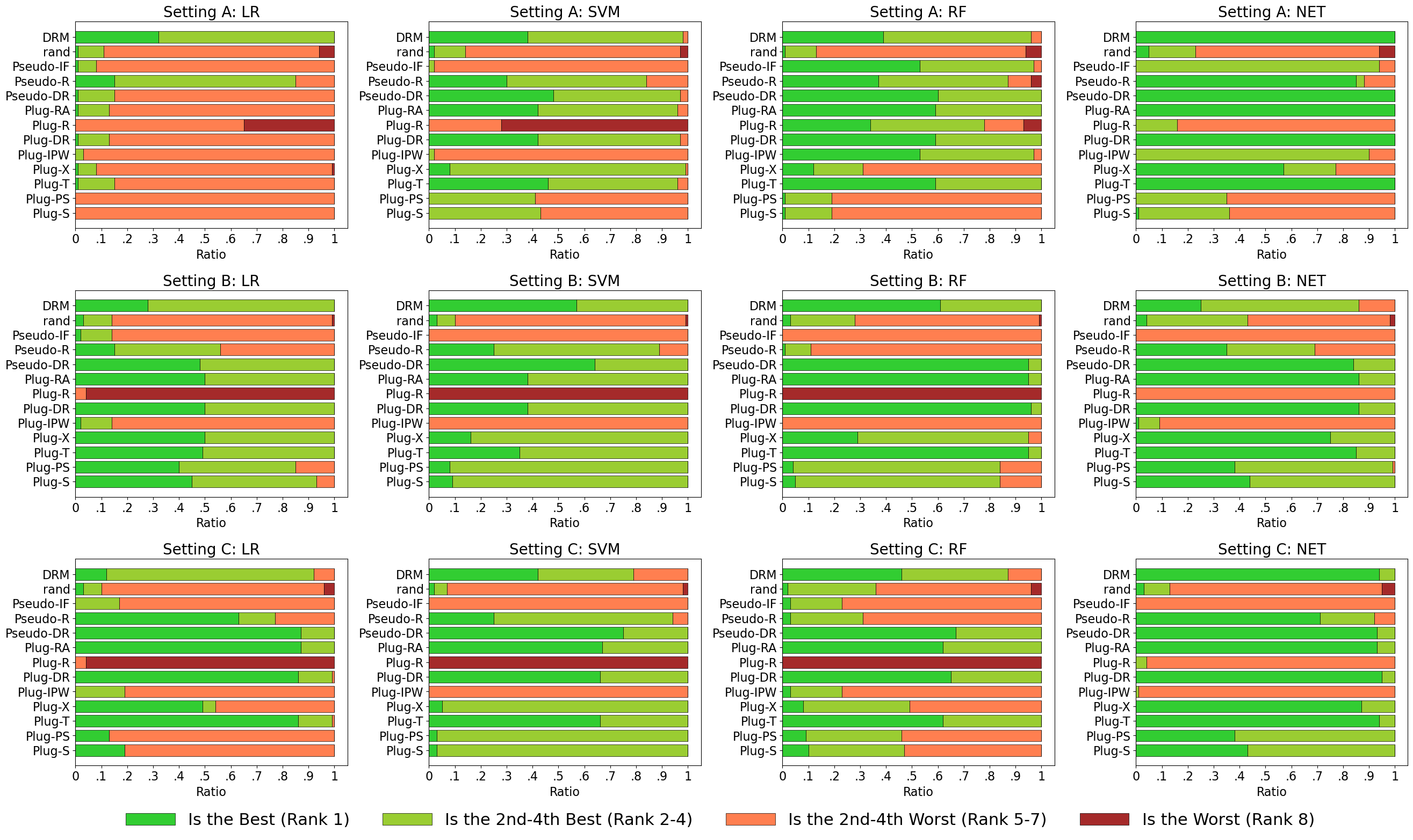
Figure 2: The stacked bar chart showing the distribution of the selected estimator’s rank for each evaluation metric across rank intervals: [1], [2-4], [5-7], [8]. The estimator selection is over 8 candidate estimators, with the underlying ML model fixed as LR, SVM, RF, or NN.

References

- Abadie et al. (2023) Abadie, A., Athey, S., Imbens, G. W., and Wooldridge, J. M. When should you adjust standard errors for clustering? The Quarterly Journal of Economics, 138(1):1–35, 2023.
- Advani et al. (2019) Advani, A., Kitagawa, T., and Słoczyński, T. Mostly harmless simulations? using monte carlo studies for estimator selection. Journal of Applied Econometrics, 34(6):893–910, 2019.
- Alaa & Van Der Schaar (2019) Alaa, A. and Van Der Schaar, M. Validating causal inference models via influence functions. In International Conference on Machine Learning, pp. 191–201. PMLR, 2019.
- Assaad et al. (2021) Assaad, S., Zeng, S., Tao, C., Datta, S., Mehta, N., Henao, R., Li, F., and Carin, L. Counterfactual representation learning with balancing weights. In International Conference on Artificial Intelligence and Statistics, pp. 1972–1980. PMLR, 2021.
- ATHEY et al. (2019) ATHEY, S., TIBSHIRANI, J., and WAGER, S. Generalized random forests. The Annals of Statistics, 47(2):1148–1178, 2019.
- Athey et al. (2021) Athey, S., Imbens, G. W., Metzger, J., and Munro, E. Using wasserstein generative adversarial networks for the design of monte carlo simulations. Journal of Econometrics, 2021.
- Bica & van der Schaar (2022) Bica, I. and van der Schaar, M. Transfer learning on heterogeneous feature spaces for treatment effects estimation. Advances in Neural Information Processing Systems, 35:37184–37198, 2022.
- Bica et al. (2021) Bica, I., Alaa, A. M., Lambert, C., and Van Der Schaar, M. From real-world patient data to individualized treatment effects using machine learning: current and future methods to address underlying challenges. Clinical Pharmacology & Therapeutics, 109(1):87–100, 2021.
- Bottou et al. (2013) Bottou, L., Peters, J., Quiñonero-Candela, J., Charles, D. X., Chickering, D. M., Portugaly, E., Ray, D., Simard, P., and Snelson, E. Counterfactual reasoning and learning systems: The example of computational advertising. Journal of Machine Learning Research, 14(11), 2013.
- Chen & Guestrin (2016) Chen, T. and Guestrin, C. Xgboost: A scalable tree boosting system. In Proceedings of the 22nd acm sigkdd international conference on knowledge discovery and data mining, pp. 785–794, 2016.
- Chernozhukov et al. (2018) Chernozhukov, V., Chetverikov, D., Demirer, M., Duflo, E., Hansen, C., Newey, W., and Robins, J. Double/debiased machine learning for treatment and structural parameters, 2018.
- Chu et al. (2021) Chu, Z., Rathbun, S. L., and Li, S. Graph infomax adversarial learning for treatment effect estimation with networked observational data. In Proceedings of the 27th ACM SIGKDD Conference on Knowledge Discovery & Data Mining, pp. 176–184, 2021.
- Curth & van der Schaar (2021a) Curth, A. and van der Schaar, M. On inductive biases for heterogeneous treatment effect estimation. Advances in Neural Information Processing Systems, 34:15883–15894, 2021a.
- Curth & van der Schaar (2021b) Curth, A. and van der Schaar, M. Nonparametric estimation of heterogeneous treatment effects: From theory to learning algorithms. In International Conference on Artificial Intelligence and Statistics, pp. 1810–1818. PMLR, 2021b.
- Curth & Van Der Schaar (2023) Curth, A. and Van Der Schaar, M. In search of insights, not magic bullets: Towards demystification of the model selection dilemma in heterogeneous treatment effect estimation. In Proceedings of the 40th International Conference on Machine Learning, volume 202 of Proceedings of Machine Learning Research, pp. 6623–6642. PMLR, 23–29 Jul 2023.
- Curth et al. (2021) Curth, A., Svensson, D., Weatherall, J., and van der Schaar, M. Really doing great at estimating cate? a critical look at ml benchmarking practices in treatment effect estimation. In Thirty-fifth conference on neural information processing systems datasets and benchmarks track (round 2), 2021.
- Donnelly et al. (2021) Donnelly, R., Blei, D., Athey, S., et al. Correction to: Counterfactual inference for consumer choice across many product categories. Quantitative Marketing and Economics, 19(3-4):409–409, 2021.
- Dorie et al. (2019) Dorie, V., Hill, J., Shalit, U., Scott, M., and Cervone, D. Automated versus do-it-yourself methods for causal inference: Lessons learned from a data analysis competition. Statistical Science, 34(1):43–68, 2019.
- Farrell (2015) Farrell, M. H. Robust inference on average treatment effects with possibly more covariates than observations. Journal of Econometrics, 189(1):1–23, 2015.
- Fernández-Loría et al. (2023) Fernández-Loría, C., Provost, F., Anderton, J., Carterette, B., and Chandar, P. A comparison of methods for treatment assignment with an application to playlist generation. Information Systems Research, 34(2):786–803, 2023.
- Foster & Syrgkanis (2023) Foster, D. J. and Syrgkanis, V. Orthogonal statistical learning. The Annals of Statistics, 51(3):879–908, 2023.
- Foster et al. (2011) Foster, J. C., Taylor, J. M., and Ruberg, S. J. Subgroup identification from randomized clinical trial data. Statistics in medicine, 30(24):2867–2880, 2011.
- Guo et al. (2020) Guo, R., Cheng, L., Li, J., Hahn, P. R., and Liu, H. A survey of learning causality with data: Problems and methods. ACM Computing Surveys (CSUR), 53(4):1–37, 2020.
- Guo et al. (2021) Guo, R., Li, J., Li, Y., Candan, K. S., Raglin, A., and Liu, H. Ignite: A minimax game toward learning individual treatment effects from networked observational data. In Proceedings of the Twenty-Ninth International Conference on International Joint Conferences on Artificial Intelligence, pp. 4534–4540, 2021.
- Hahn et al. (2020) Hahn, P. R., Murray, J. S., and Carvalho, C. M. Bayesian regression tree models for causal inference: Regularization, confounding, and heterogeneous effects (with discussion). Bayesian Analysis, 15(3):965–1056, 2020.
- Hassanpour & Greiner (2019) Hassanpour, N. and Greiner, R. Learning disentangled representations for counterfactual regression. In International Conference on Learning Representations, 2019.
- Hill (2011) Hill, J. L. Bayesian nonparametric modeling for causal inference. Journal of Computational and Graphical Statistics, 20(1):217–240, 2011.
- Holland (1986) Holland, P. W. Statistics and causal inference. Journal of the American statistical Association, 81(396):945–960, 1986.
- Hu & Hong (2013) Hu, Z. and Hong, L. J. Kullback-leibler divergence constrained distributionally robust optimization. Available at Optimization Online, 1(2):9, 2013.
- Huang et al. (2021) Huang, Y., Leung, C. H., Yan, X., Wu, Q., Peng, N., Wang, D., and Huang, Z. The causal learning of retail delinquency. In Proceedings of the AAAI Conference on Artificial Intelligence, volume 35, pp. 204–212, 2021.
- Huang et al. (2023) Huang, Y., Leung, C. H., Ma, S., Yuan, Z., Wu, Q., Wang, S., Wang, D., and Huang, Z. Towards balanced representation learning for credit policy evaluation. In International Conference on Artificial Intelligence and Statistics, pp. 3677–3692. PMLR, 2023.
- Johansson et al. (2016) Johansson, F., Shalit, U., and Sontag, D. Learning representations for counterfactual inference. In International conference on machine learning, pp. 3020–3029. PMLR, 2016.
- Johansson et al. (2022) Johansson, F. D., Shalit, U., Kallus, N., and Sontag, D. Generalization bounds and representation learning for estimation of potential outcomes and causal effects. The Journal of Machine Learning Research, 23(1):7489–7538, 2022.
- Kennedy (2023) Kennedy, E. H. Towards optimal doubly robust estimation of heterogeneous causal effects. Electronic Journal of Statistics, 17(2):3008–3049, 2023.
- Kinyanjui & Johansson (2022) Kinyanjui, N. M. and Johansson, F. D. Adcb: An alzheimer’s disease simulator for benchmarking observational estimators of causal effects. In Conference on Health, Inference, and Learning, pp. 103–118. PMLR, 2022.
- Kitagawa & Tetenov (2018) Kitagawa, T. and Tetenov, A. Who should be treated? empirical welfare maximization methods for treatment choice. Econometrica, 86(2):591–616, 2018.
- Kuang et al. (2017) Kuang, K., Cui, P., Li, B., Jiang, M., Yang, S., and Wang, F. Treatment effect estimation with data-driven variable decomposition. In Proceedings of the AAAI Conference on Artificial Intelligence, volume 31, 2017.
- Kuang et al. (2020) Kuang, K., Cui, P., Zou, H., Li, B., Tao, J., Wu, F., and Yang, S. Data-driven variable decomposition for treatment effect estimation. IEEE Transactions on Knowledge and Data Engineering, 34(5):2120–2134, 2020.
- Kuhn et al. (2019) Kuhn, D., Esfahani, P. M., Nguyen, V. A., and Shafieezadeh-Abadeh, S. Wasserstein distributionally robust optimization: Theory and applications in machine learning. In Operations research & management science in the age of analytics, pp. 130–166. Informs, 2019.
- Künzel et al. (2019) Künzel, S. R., Sekhon, J. S., Bickel, P. J., and Yu, B. Metalearners for estimating heterogeneous treatment effects using machine learning. Proceedings of the national academy of sciences, 116(10):4156–4165, 2019.
- Levy et al. (2020) Levy, D., Carmon, Y., Duchi, J. C., and Sidford, A. Large-scale methods for distributionally robust optimization. Advances in Neural Information Processing Systems, 33:8847–8860, 2020.
- Li & Wager (2022) Li, S. and Wager, S. Random graph asymptotics for treatment effect estimation under network interference. The Annals of Statistics, 50(4):2334–2358, 2022.
- Louizos et al. (2017) Louizos, C., Shalit, U., Mooij, J. M., Sontag, D., Zemel, R., and Welling, M. Causal effect inference with deep latent-variable models. Advances in neural information processing systems, 30, 2017.
- Ma et al. (2020) Ma, S., Leung, C. H., Wu, Q., Liu, W., and Peng, N. Understanding distributional ambiguity via non-robust chance constraint. In Proceedings of the First ACM International Conference on AI in Finance, pp. 1–8, 2020.
- Mahajan et al. (2024) Mahajan, D., Mitliagkas, I., Neal, B., and Syrgkanis, V. Empirical analysis of model selection for heterogenous causal effect estimation. International Conference on Learning Representations, 2024.
- Mohajerin Esfahani & Kuhn (2018) Mohajerin Esfahani, P. and Kuhn, D. Data-driven distributionally robust optimization using the wasserstein metric: performance guarantees and tractable reformulations. Mathematical Programming, 171(1-2):115–166, 2018.
- Nie & Wager (2021) Nie, X. and Wager, S. Quasi-oracle estimation of heterogeneous treatment effects. Biometrika, 108(2):299–319, 2021.
- Nogueira et al. (2022) Nogueira, A. R., Pugnana, A., Ruggieri, S., Pedreschi, D., and Gama, J. Methods and tools for causal discovery and causal inference. Wiley interdisciplinary reviews: data mining and knowledge discovery, 12(2):e1449, 2022.
- Noh et al. (2014) Noh, Y.-K., Sugiyama, M., Liu, S., Plessis, M. C., Park, F. C., and Lee, D. D. Bias reduction and metric learning for nearest-neighbor estimation of kullback-leibler divergence. In Artificial Intelligence and Statistics, pp. 669–677. PMLR, 2014.
- Oprescu et al. (2019) Oprescu, M., Syrgkanis, V., and Wu, Z. S. Orthogonal random forest for causal inference. In International Conference on Machine Learning, pp. 4932–4941. PMLR, 2019.
- Parikh et al. (2022) Parikh, H., Varjao, C., Xu, L., and Tchetgen, E. T. Validating causal inference methods. In International Conference on Machine Learning, pp. 17346–17358. PMLR, 2022.
- Pflug (2023) Pflug, G. C. Multistage stochastic decision problems: Approximation by recursive structures and ambiguity modeling. European Journal of Operational Research, 306(3):1027–1039, 2023.
- Qian et al. (2021) Qian, Z., Zhang, Y., Bica, I., Wood, A., and van der Schaar, M. Synctwin: Treatment effect estimation with longitudinal outcomes. Advances in Neural Information Processing Systems, 34:3178–3190, 2021.
- Rosenbaum & Rubin (1983) Rosenbaum, P. R. and Rubin, D. B. The central role of the propensity score in observational studies for causal effects. Biometrika, 70(1):41–55, 1983.
- Rubin (2005) Rubin, D. B. Causal inference using potential outcomes: Design, modeling, decisions. Journal of the American Statistical Association, 100(469):322–331, 2005.
- Schuler et al. (2017) Schuler, A., Jung, K., Tibshirani, R., Hastie, T., and Shah, N. Synth-validation: Selecting the best causal inference method for a given dataset. arXiv preprint arXiv:1711.00083, 2017.
- Schuler et al. (2018) Schuler, A., Baiocchi, M., Tibshirani, R., and Shah, N. A comparison of methods for model selection when estimating individual treatment effects. arXiv preprint arXiv:1804.05146, 2018.
- Shalit et al. (2017) Shalit, U., Johansson, F. D., and Sontag, D. Estimating individual treatment effect: generalization bounds and algorithms. In International conference on machine learning, pp. 3076–3085. PMLR, 2017.
- Shi et al. (2019) Shi, C., Blei, D., and Veitch, V. Adapting neural networks for the estimation of treatment effects. Advances in neural information processing systems, 32, 2019.
- Wager & Athey (2018) Wager, S. and Athey, S. Estimation and inference of heterogeneous treatment effects using random forests. Journal of the American Statistical Association, 113(523):1228–1242, 2018.
- Wang et al. (2021) Wang, J., Gao, R., and Xie, Y. Sinkhorn distributionally robust optimization. arXiv preprint arXiv:2109.11926, 2021.
- Wang et al. (2006) Wang, Q., Kulkarni, S. R., and Verdú, S. A nearest-neighbor approach to estimating divergence between continuous random vectors. In 2006 IEEE International Symposium on Information Theory, pp. 242–246. IEEE, 2006.
- Wu et al. (2022) Wu, A., Yuan, J., Kuang, K., Li, B., Wu, R., Zhu, Q., Zhuang, Y., and Wu, F. Learning decomposed representations for treatment effect estimation. IEEE Transactions on Knowledge and Data Engineering, 35(5):4989–5001, 2022.
- Yao et al. (2018) Yao, L., Li, S., Li, Y., Huai, M., Gao, J., and Zhang, A. Representation learning for treatment effect estimation from observational data. Advances in neural information processing systems, 31, 2018.
- Yao et al. (2021) Yao, L., Chu, Z., Li, S., Li, Y., Gao, J., and Zhang, A. A survey on causal inference. ACM Transactions on Knowledge Discovery from Data (TKDD), 15(5):1–46, 2021.
- Yoon et al. (2018) Yoon, J., Jordon, J., and Van Der Schaar, M. Ganite: Estimation of individualized treatment effects using generative adversarial nets. In International conference on learning representations, 2018.
- Zhang et al. (2019) Zhang, L., Wang, Y., Ostropolets, A., Mulgrave, J. J., Blei, D. M., and Hripcsak, G. The medical deconfounder: assessing treatment effects with electronic health records. In Machine Learning for Healthcare Conference, pp. 490–512. PMLR, 2019.
- Zhang et al. (2020) Zhang, Y., Bellot, A., and Schaar, M. Learning overlapping representations for the estimation of individualized treatment effects. In International Conference on Artificial Intelligence and Statistics, pp. 1005–1014. PMLR, 2020.