FSL Model can Score Higher as It Is

Abstract

In daily life, we tend to present the front of our faces by staring squarely at a facial recognition machine, instead of facing it sideways, in order to increase the chance of being correctly recognised. Few-shot-learning (FSL) classification is challenging in itself because a model has to identify images that belong to classes previously unseen during training. Therefore, a warped and non-typical query or support image during testing can make it even more challenging for a model to predict correctly. In our work, to increase the chance of correct prediction during testing, we aim to rectify the test input of a trained FSL model by generating new samples of the tested classes through image-to-image translation. An FSL model is usually trained on classes with sufficient samples, and then tested on classes with few-shot samples. Our proposed method first captures the style or shape of the test image, and then identifies a suitable trained class sample. It then transfers the style or shape of the test image to the train-class images for generation of more test-class samples, before performing classification based on a set of generated samples instead of just one sample. Our method has potential in empowering a trained FSL model to score higher during the testing phase without any extra training nor dataset. According to our experiments, by augmenting the support set with just 1 additional generated sample, we can achieve around $2\%$ improvement for trained FSL models on datasets consisting of either animal faces or traffic signs. By augmenting both the support set and the queries, we can achieve even more performance improvement. Our Github Repository is publicly available.

Figure 1: Illustration of the FSL rectifier effect, which can push a randomly sampled point closer to the centroid of its class. As discussed, being closer to the centroid can increase the chance of successful classification. In this figure, we generate 4 TSNE [27] projections, using the same set of data and different TSNE seeds (0, 1, 2 and 3 respectively). More details in Section 6.1.

Figure 2: Illustration of the image translator effect with the Animals (left) and traffic signs (right) datasets. The first image in each column of the animals dataset is the original test-sample, the second is neighbour sample from the test class. For the Animals, the last image is the generation based on style of original test-sample and shape of neighbour. For the traffic signs, the first row is the original test-sample, the second row is the reconstructed samples, and remaining images are generated based on style of neighbour and shape of original test-sample.

1 Introduction

Traditionally, machine learning trains a model to identify unseen images of a learnt (seen) class. In Few-Shot Learning (FSL), however, models usually have to identify new images from an unseen class when presented with a support set comprising only a few shots of labeled samples as reference [35]. In general, FSL models perform much better when the support set contains more labeled examples, which lead to a more robust and typical representation (e.g. A 5-shot set-up achieves better performance than a 1-shot set-up) [35, 38]. In a similar vein, a trained model tends to perform better when it is presented with “familiar and standard” input, since the model learns from many more typical (i.e. near to the class centroid) data samples as opposed to outliers of the class. For instance, if a model is only trained on a set of standing, front-facing dog images, it may have difficulty representing and classifying a side-facing swimming wolf sample. In other words, where models are presented with support samples or queries from unseen classes, unusual angles of the queried object or support samples can exacerbate the challenges faced by a model in few-shot classification tasks [25].

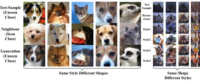
With this backdrop, we design a scheme to “rectify” images used during FSL testing phase. To rectify the image inputs, we first identify a suitable sample, denoted as the “neighbour sample”, used during training. Then, we generate additional test-samples that merge the “shapes” and “syles” of the neighbour sample and original test-sample. In our context, shape refers to the primary features of an image (e.g. pose, location of eyes and nose of animal faces, traffic sign patterns), and style refers to the secondary features (e.g. fur looks, lighting on traffic sign boards) . Finally, we perform classification based on the entire set of generated test-class images, along with the original test-sample. Using the aforementioned side-facing swimming wolf example, we can extract the class-defining style of the typical front-facing dogs and apply the style to those swimming wolves, i.e. converting the side-facing swimming wolves to front-facing standing wolves using an image translation model, before finally performing the few-shot classification. On the other hand, we can also graft the styles of train class images onto test-class-shaped images to produce more test-class samples, when the dataset is defined by shape rather than styles. Whether a style or shape should be extracted depends on the nature of the datasets. Based on our implementation and experiments, such a scheme can be effective in enhancing the performance of an already trained FSL model.

Generative techniques form an important direction in the FSL research community. For example, in [23, 14, 3, 9], new image samples are generated to augment the training class. However, most of the prior works only consider augmenting the training classes with more training data. As the generation takes place during the training phase, a model has to be trained to improve. Our approach is different in that it uses augmentation and rectification during the testing phase. To summarize, in this work, we propose a method to augment the test inputs instead of the training samples, thus enabling a trained FSL model to score higher in a test without modifying or training the model itself.

2 Preliminary: Few-Shot Learning

FSL finds its real-life applications in enabling a model to classify an unseen class of data points when given only a few labeled samples of the unseen class [35]. Generally, in an FSL classification set-up, an FSL model compares the queried samples against the labeled references to predict which class the queries belong to. For example, in FSL, a model may be presented with one picture of a cat. The model is not trained on cat classes, but has seen classes like wolf or tiger. Meanwhile, the model is presented with a support set, where using the aforementioned example, would be samples consisting of labeled pictures of cats and other unseen-class objects. The FSL model then compares the queries against the labeled support set samples to predict which queries are cats [35]. This makes FSL suitable for real-world applications where data collection, especially for the rare classes, can be expensive.

In FSL, models are usually trained on one set of classes called the train split, and tested on another set of classes called the test split, with the two splits not sharing any common classes. During both training and testing phases, an FSL model is usually trained and tested through “episodes”, where “episodic sampling” is adopted. Each episode, formed through episodic sampling, consists of a support set and query(ies). In this work, we refer to both the support set and queries in the testing phase as “test-samples”. Each query class is the same as one of the support set classes. Specifically, first randomly choosing $n$ classes, an episodic sampler can then sample $k$ examples from each of the $n$ chosen classes, forming an $n$-way-$k$-shot support set [35]. In this paper, for simplicity, we consider $n$-way-1-shot classification only i.e. there are $n$ support classes in total, each containing just one support sample.

3 Related Works

As mentioned in Section 2, FSL classification has a different set-up from traditional classifications [35, 19]. Mainstream algorithms include the meta-learning methodology and metric-learning methodology [35]. Related to our works, FSL algorithms include the matching network(MatchNet) [31] and the Prototypical Network(ProtoNet) [25], which measures the euclidean distance between query and support embeddings for identifying the most probable categories of the queries. Another similar algorithm called FEAT [38] incorporates a transformer [29] layer to the matching network set-up, which enhances the expressiveness of image embeddings. DeepSets [38] is a variant of the FEAT algorithm which replaces the transformer layer in FEAT with an alternative non-linear set-to-set transformation function.

In the field of test-time augmentation, there are plenty of works like [1, 8]. However, only a few are in FSL, such as  [37, 10], where the authors find that basic image transformations like cropping and resizing improve FSL model performance. In our work, while we observe similar findings, we introduce more possibilities to the augmentation.

In the field of image translation, which is a form of generative AI, there are various generative models, such as the Variational Auto-Encoder (VAE) and the Generative Adversarial Network (GAN) [16, 33]. Celebrated generative models include the CycleGAN [40], which merges two pictures through a symmetric pair of GAN networks. Other related works such as the StyleGAN [6], coco-funit/funit [22, 13] and more [17, 34] can also achieve realistic results in generating new images conditioned on different user requirements.

The use of image generation in FSL has also been explored, such as the “congealing” method which grafts variations from similar classes to a separate class [35]. Similar ideas are also seen in FSL works like [15, 30, 24, 3, 36, 2], where the authors aim to augment the training dataset to achieve better generalization among FSL models. Another work similar to ours is [9], where the authors correct the angles of traffic signs through VAE as well, setting the standard traffic signs images as the reconstruction targets of a VAE.

Our work differs from these works in many aspects. While the prior works focus on training-phase augmentation, we only focus on testing-phase augmentation for models that are already trained. More specifically, we separate styles and shapes of source images during the generation of new test-samples. Such a separation enables us to “mix and match” shapes and styles of train-split and test-split data. Through linking test inputs to train-split data, we can augment these test-samples in a meaningful way during test time, which is a novel idea to the best of our knowledge.

4 Method

This section introduces the GAN image translator, the neighbour selector and the FSL rectifier. An image translator generates new test inputs based on test-samples and neighbours selected by the neighbour selector, before the FSL rectifier considers the average of those generated images, as well as the reconstructed original test-samples.

4.1 Image Translator

Figure 3: Illustration of the rectifier augmention. There are two test-samples, on the left and right respectively, augmented to become three test-samples based on the train-split image translations.

The objective of the image translator is to translate an input image to the provided class, which can be unseen. With the generation of new samples, we augment the number of samples from the test class. Let $x$ denote the image from which we extract the shape or pose. Let $y$ denote an image from which we extract the style. The image translator $G$ consists of a shape encoder $E_{x}$, a style encoder $E_{y}$ and a decoder $F_{x}$. The style encoder captures the style and appearance of an image, and the shape encoder captures the pose and shape of another image. The image translator essentially produces images $\bar{x}$ defined by $G(x,y)=F_{x}(E_{x}(x),E_{y}(y))$.

During training, we solve the following minimax optimization problem:

$$\min_{D}\max_{G}\mathcal{L}_{\text{GAN}}(D,G)+k_{R}\mathcal{L}_{R}(G)+k_{\text{FM}}\mathcal{L}_{\text{FM}}(G)\textrm{.}$$ (1)

where $D$ is the discriminator in the GAN network, $k_{R}$ and $k_{\text{FM}}$ are hyperparemters, $\mathcal{L}_{\text{GAN}}$ is the GAN-loss, $\mathcal{L}_{R}$ is the reconstruction loss and $\mathcal{L}_{\text{FM}}$ is the feature matching loss.

The GAN-loss drives the training of both the generator and the discriminator to compete through the following objective function:

$$\begin{split}\mathcal{L}_{\text{GAN}}(D,G)=\mathbb{E}_{x}[-\log D(x)]+\mathbb{E}_{x,y}[\log(1-D(\bar{x})]\textrm{.}\end{split}$$ (2)

Here, the discriminator tries to discern between real and images produced by the generator, while encouraging the generation to become the same class as the original test-sample class through a classifier $h_{d}$ coupled with the discriminator encoder. The discriminator classifier is simply a fully connected layer with output size equal to the number of training classes. At the same time, the generator tries to fool the discriminator.

The reconstruction loss $\mathcal{L}_{R}$ helps generator $G$ generate outputs that resemble the shape of the target images, which are designed as the input images themselves in the loss function:

$$\mathcal{L}_{R}(G)=\mathbb{E}_{x}[\|x-G(x,x)\|^{1}_{1}]\textrm{.}$$ (3)

The feature matching loss helps regularize the training, generating new samples that possess the style of the image $y$:

$$\begin{split}\mathcal{L}_{\text{FM}}(G)=\mathbb{E}_{x,y}\left[\|D_{f}\left(\bar{x}\right)-D_{f}(y)\|^{1}_{1}\right]\textrm{.}\end{split}$$ (4)

Here, $D_{f}$ is the feature extractor, which is obtained from removing the last layer (the classifier layer) from $D$.

The shape encoder is made of convolutional layers and residual blocks, converting input images to their latent representations. The style encoder consists of convolutional layers followed by an averaging operation, mapping several images to their latent representations before averaging them. The decoder consists of a few adaptive instance normalization (AdaIN) residual blocks [5] followed by upscaling using convolutional layers [12]. This image translator, including the reconstruction loss and feature matching loss, are adopted from [22, 12, 11, 17, 34]. Lastly, during training of the image translator, we only use the train-split of a dataset, leaving the test-split dataset unseen.

4.2 Neighbour Selector

Image translator as a generative model can at times produce poor results (See Section 6.2 and Appendix). Furthermore, it can be fallacious to presume that features among different classes can always be mix-and-matched in meaningful ways. To ensure that the good-quality generations are used during the testing phase, we introduce the “neighbour selector” which, when presented with a pool of candidate neighbour images, can return the better candidates for the generation of new test-samples.

Intuitively, a naive way to implement this neighbour selector is to generate new test-samples based on each neighbour candidate, before selecting the best generated sample based on a measure of generation quality like those in [32]. However, it can be computationally expensive to generate all these images and then assess their quality individually.

For higher efficiency and practicality, we train a neighbour selector using randomly sampled datapoints from both the training set, which is denoted as $\mathcal{D}_{\text{train}}$, and the testing set, $\mathcal{D}_{\text{test}}$, without any supervision information. Reusing the trained image translator, we aim to update the shape encoder $E_{x}$ to becom $E_{f}$ such that, for a pair of original test-sample $y\in\mathcal{D}_{\text{test}}$ and neighbour $x\in\mathcal{D}_{\text{train}}$, $E_{f}(x)\cdot E_{f}(y)$ returns a “generation quality” score, which estimates the quality of generation for $G(x,y)$. To achieve this, during training of $E_{f}$, we feed combinations of test-samples and neighbours $\{x,y\}$ and minimize the following objective function $\mathcal{L}_{\text{KL}}$, defined by

Here, $\sigma$ is the softmax function, $h_{d}(\cdot)$ represents the logits output from the trained and frozen classifier $h_{d}$ in discriminator $D$. The idea is to obtain an encoder which produces query/support-neighbour features that, when multiplied in a pairwise manner, indicates the KL-Divergence between the generation class prediction and original test-sample class prediction. In other words, we judge whether a generation is good through how much our trained classifier in $D$ classifies the original test-sample and generated sample as the same object. During actual testing, a candidate neighbour sample $x$, whose feature leading to the lowest divergence score when multiplied with the original test-sample feature $E_{f}(y)$, is selected from a pool of neighbour candidates $\{x^{\prime}\}$. i.e.:

$$x=\operatorname*{argmin}_{x^{\prime}}E_{f}(x^{\prime})\cdot E_{f}(y)\textrm{.}$$ (6)

To summarize, we aim to represent pairwise feature products as a quality indicator, so that we can select the better neighbours without the actual generation. Meanwhile, the same configuration for the image translator is used, keeping our solution simplistic.

4.3 FSL Rectifier

“FSL rectifier” is our main proposed method, encompassing both the aforementioned image translator and neighbour selector. During the testing phase, all input images are augmented to form multiple images of the same class. The augmentation is produced by the image translator, based on both test-samples and train-samples selected by the neighbour selector. The multiple copies are then averaged to form a “rectified” representation of the original test input. Specifically, we generate $k$ samples for each test input and consider the average representation of these $k$ samples for $n$-way-1-shot classification. Depending on the nature of the dataset, FSL rectifier generates new samples by either combining shape of train-class samples and style of test-class samples, or combining shape of test-class samples and style of train-class samples. Lastly, the trained FSL model uses the average representation of the set of generated images coupled with the reconstructed original test-sample to make a prediction.

Let $R_{k}$ denote the FSL rectifier which generates $k$ new samples, $h$ the trained FSL model whose performance we aim to improve, and $h^{\prime}$ the classifier which shares the same encoder $\phi$ as the trained FSL model $h$. The FSL rectifier is a function which translates one image sample $z$ to $k$ copies of generated images, before considering their average embeddings. When the FSL rectifier combines style of train-class samples and shape of test-samples, it can be defined as below:

$$\begin{split}R_{k}:z\rightarrow&\frac{1-\beta}{k}\sum\{\phi(G(z,v_{1})),...\phi(G(z,v_{k}))\}+\\ &\beta\cdot\phi(G(z,z))\textrm{.}\end{split}$$ (7)

where $z$ is the test-sample, $\{v_{i}\}$ are train-class samples and $\beta$ is the weight placed on the reconstruction of the original test-sample. When the FSL rectifier combines shape of train-class samples and style of test-samples, it produces a set of images defined by $\{G(v_{1},z),...G(v_{k},z)\}$. Final FSL predictions can be rendered based on:

$$\hat{y}=h^{\prime}(R_{k}(q)|\{R_{k}(s_{1}),...R_{k}(s_{n})\})\textrm{.}$$ (8)

where $q$ represents the query image and $s$ represents each support set image.

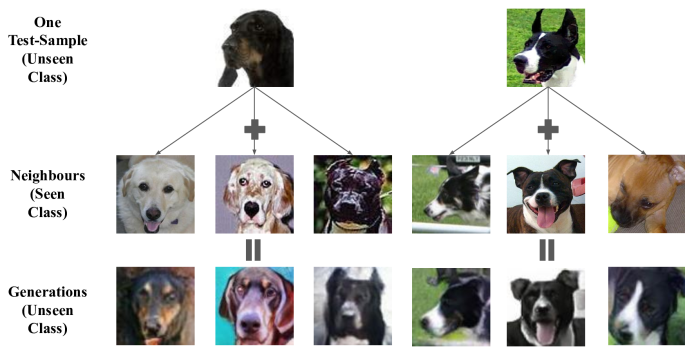
In this work, we consider two datasets consisting of traffic signs and of animal faces. For the traffic signs dataset, we extract the styles of train-class samples and combine them with test-class-image shapes. This is because that traffic signs are defined by shapes (i.e. patterns printed) rather than styles (e.g. lighting over the sign boards). However, for the animal faces dataset, we extract the major shapes or poses of train-class samples and combine them with test-input style. This is because similar classes of animal faces tend to have similar major shapes (e.g. facial features like location of eyes and nose) but different styles (e.g. fur and overall looks). Examples of the translations are illustrated by Figure 2. Examples of how one image gets augmented to form multiple images are illustrated by Figure 3.

5 Implementation and Experiment

This section specifies the primary implementation and experiment details regarding our works. More details can be found in Appendix.

5.1 Datasets

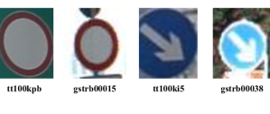
In this work, we use the animal faces (Animals) datasets, consisting of 117,574 carnivorous animal facial images sub-sampled from the ImageNet [21, 13] dataset. There are 129 classes in total, 119 of which belong to the train split and 30 the test split. Besides, we also have the traffic signs datasets, consisting of two sets of real-world traffic signs patterns called GTSRB [41] and TT100K [26] respectively. This dataset has 37,678 images for the train split from 61 different classes, and 13,517 images for the test split from 16 different classes. All images from these datasets are colored and resized to 128$\times$128 dimension during training and testing. As there are many dark images in this dataset, we preprocess it through the Contrast Limited Adaptive Histogram Equalization (CLAHE) [28, 7] algorithm when training both the image translator and the FSL model. However, we feed original samples without CLAHE preprocessing when testing different FSL algorithms, making the classification task more challenging. To study the effect of augmention explicitly, we compare test-samples reconstructed by the image translator, with or without augmentions. The reconstruction examples include test-samples in Figure 2 and Figure 5.

5.2 Models

To obtain trained FSL models used in this work, we use the Prototypical Network [25], the FEAT, and the DeepSets [38] with either a euclidean-distance or cosine-similarity classifier for experiments. Our experiments pair the algorithms with both Conv4 and Res12 [4] encoders, which we adopt from [38]. We conduct pretraining of both of these encoders before training them further on different FSL algorithms.

For the training of the GAN-based image image translator, we set the maximum training iteration to 100,000, batch size to 64, and learning rate for both the discriminator and generator to 0.0001. When training the neighbour selector, we clone a copy of the trained image translator. The learning rate is set to 0.001, and the maximum training iterations is 200.

When testing the FSL rectifier against the baseline, we pass the same 5,000 5-way-1-shot queries to the same trained FSL model. The neighbour selector considers 20 candidates for each neighbour selection. To obtain our reported results for Animals, as the original test-sample tends be of the best-quality, we place double weight on the original-test-sample when averaging the original samples and the augmented samples. All 95% confidence intervals are around our reported results $\pm$0.9%.

5.3 Baselines

Our baselines include: 1. One-Shot: based on the original support set; 2. Mix-Up: based on an augmented support set consisting of both the original support set and the neighbours selected by neighbour-selector; 3-5. Crop-Rotate/Affine/Color-Jitter: based on various augmentations adopted from the Pytorch transform functions [18].

5.4 Main Experiment

Table 1 consists of experimental results of our proposed method. All results in the table are accuracy scores of a 5-way-1-shot set-up. The light-gray columns represent the traffic-sign results, and the darker-gray columns represent the Animals results. For each support set, we only augment each support sample with just 1 additional copy of generation, keeping queries untouched. Based on the experimental results, our method can be effective especially for both datasets, and the improvement is around 2%. Its performance is also better when compared to other augmentation techniques in general. Nevertheless, we highlight that rectification results are dataset-dependent, and the improvement brought by the different techniques can differ when applied in different datasets. For example, we observe that other forms of augmentation, such as Crop-Rotate, may work for the Animals dataset, but not the traffic dataset. This can be explained by the fact that rotating certain traffic signs can change them to other classes. Additionally, for the Animals dataset, other forms of augmentations such as Crop-Rotate and Affine are also helpful in enhancing test-time performance, which is corroborated in other works [10, 37].

		ProtoNet-Cos (%)		ProtoNet-Euc (%)
One-Shot	Conv4	50.25	40.40	51.00	41.27
	Res12	64.24	61.07	65.95	62.87
Mix-Up	Conv4	51.24	34.33	51.93	35.01
	Res12	65.55	-	66.81	-
Crop-Rotate	Conv4	51.76	36.07	55.89	35.94
	Res12	61.27	55.92	61.50	55.47
Affine	Conv4	51.49	38.01	52.20	39.43
	Res12	64.87	55.58	64.58	55.99
Color-Jitter	Conv4	42.97	36.48	43.28	36.50
	Res12	56.39	52.40	55.89	53.11
Ours	Conv4	52.85	42.26	53.33	43.41
	Res12	66.38	62.96	67.85	64.50

Table 1: Main experiment results. The light-gray columns represent the traffic-sign results, and the darker-gray columns represent the Animals results. The red numbers indicate the results for Conv4 encoder. The blue numbers indicate those for Res12 encoder. “Cos” and “Euc” respectively represents a cosine-similarity-based classifier and a euclidean-distance-based classifier.

5.5 Query Augmentation

Augmentation Copies	(Support) 0	1	2	3
(Query) 0	50.04±0.87	51.83±0.86	51.94±0.94	52.26±0.97
1	65.73±0.87	94.80±0.63	93.46±0.69	91.92±0.75
2	70.80±0.94	96.80±0.50	99.74±0.14	99.54±0.19
3	72.82±1.16	96.84±0.48	99.70±0.15	99.98±0.14

Table 2: 5-way-1-shot accuracy on how the sizes of augmentation for both the support set and queries affect the test accuracy in the Animals dataset.

When we augment the testing data, a natural question arising is how many new samples we should generate to achieve a desired level of performance, and whether we should augment the support set, or the queries, or both. To study the effect of query augmentation, we augment each input query with less or equal to 3 additional copies. Then, we perform simple-averaging over FSL embeddings of all augmented copies as well as the reconstructed original test-sample input i.e. we place the same weight on the reconstructed original test-sample input as that we place on any other augmentation. Meanwhile, we pair the augmented queries with support sets augmented with less or equal to 3 additional copies, which are also combined via the simple-averaging. Table 2 indicates the 5-way-1-shot classification accuracy we have for all the different set-ups. The experiment is done on both the Animals dataset and the traffic signs dataset, using the Prototypical Network [25] coupled with a cosine-similarity-based classifier. Based on the result, we observe that query augmentation can be effective, especially when coupled with support set augmentation; we can ace the 5-way-1-shot classification task on these two datasets when the augmentation size is around 2 or 3 copies, reaching almost 100% accuracy. Besides, we observe that query augmentation can be even more effective than support set augmentation, as the marginal increase of accuracy score brought by each query augmentation is much higher than that brought by the support set augmentation.

6 Further Discussions and Ablation Studies

This section studies the ablative variants of our proposed method and discusses the method further.

6.1 Is the Combined Sample Better

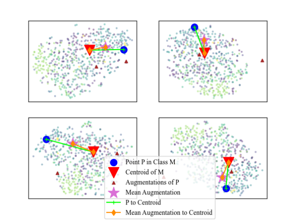
To study whether the combined representation of multiple generated samples can be better, we perform the TSNE [27] projection before and after applying FSL-Rectification. The results are reflected in Figure 1. In this figure, each projection represents the same subset of datapoints randomly sampled from 10 different classes in the Animals [21, 12] dataset. The blue point is a randomly sampled datapoint. This datapoint, along with its neighbour samples, is used to generate new samples using our proposed method FSL rectifier. The pink star represents the average of the newly generated samples, which is generally closer to the centroid compared to the original datapoint. It is clear that the combined samples are more easily recognizable, and one way to explain is that samples near the centroid tend to be more well-separated from other classeses  [25]. Features of the sampled datapoints are produced by the Conv4 [38] encoder trained through the Prototypical Network [25, 38] algorithm, and the number of new samples generated for the datapoint considered is 5. Due to representational limitations of projection, we generate multiple projections using different random seeds for TSNE, in a bid to ensure the consistency of performance. We repeat the TSNE projections multiple times using different seeds, and the “nearer-to-centroid” effect is observed in all our trials.

6.2 Ablation Studies and Failure Cases

Figure 4: Illustration of failure cases of Animals dataset without the neighbour selector. At the bottom is the original image where generations above are based on. The generated images tend to have the wrong colour or shape, or are blurry.

Figure 5: Illustration of the effect of neighbour selector. For the Animals dataset, the first row is the original-test-sample and the third row is the new test-sample generated by the image translator. For the traffic signs dataset, the first row is the original-test-sample, the second row is its reconstruction, and remaining rows are augmentations in different styles. For the Animals dataset, we consider 3 pairs of generations under either the inverse neighbour selector or the standard neighbour selector used in our method. Within each pair, the neighbour image on the left is the worst, and the one on the right is the best, as perceived by our proposed neighbour selector.

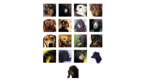
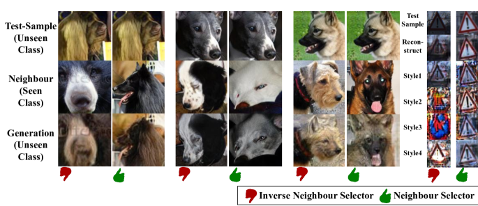
There are a few failure cases of our image translator, which are illustrated in Figure 4. For example, for a dog image at the bottom of Figure 4, some generations are indecipherable. Therefore, improving the quality of image generation via more advanced approaches [20] or detecting failure cases in generation may further enhance the performance of the test-time augmentation. To study the importance of our neighbour selector, we first visualize the neighbours and generations rendered by an “Inverse neighbour selector” and the original neighbour selector. To recap, the neighbour selector sorts a set of candidate neighbours from good to bad, and returns the first $k$ copies of the candidate neighbour samples for the actual image generation. The Inverse neighbour selector is the same as the neighbour selector, except that it returns the $k$ samples deemed to be the worst. The contrast is presented in Figure 5, which demonstrates that the neighbour selector can improve the quality of generation. This observation is further confirmed in Table 3, where the neighbour selector improves the test accuracy. In this study, we set the number of neighbour candidates to consider for each generation to 40. We observe that the higher the value, the more salient the effect of neighbour selector in general. However, we also observe that the marginal improvement in generation quality diminishes when the number of neighbour candidates increases. Additionally, we believe that the neighbour selector can be even more important in many other datasets, where the chance of failure for image translation tend to be higher.

Furthermore, to study the effectiveness of image translation, we replace the translation with mix-up, which simply returns a combination of the neighbour sample and the test-sample at the raw image level. Interestingly, such an augmentation strategy can work when the neighbour selector is in place, though not performing as well as an image translator. Nevertheless, it can be an option to consider in the face of limited computation resources.

Lastly, we also consider Crop-Rotate and its combination with our method. In our main experiment 1, we place double weight on the original test-sample. In other words, previously, each augmentation consists of an original test-sample and an generated sample. In this study, we replace each original test-sample with its cropped and rotated version. Based on our experiments, the different augmentation methods can be effective, and combining them can be even more effective. Usually, a combination of methods can perform better than its own individual component especially when the individual method tend to be dissimilar in nature compared with one another [39]. Therefore, we believe this improvement can be attributed to the high degree of dissimilarity between our method and Crop-Rotate. There are many non-deep test-time augmentation techniques [37, 8], and our augmentation technique has the potential to complement these non-deep techniques. Other possible combinations can be explored in future works.

neighbour selector	image translator	Crop-Rotate	Accuracy (%)
✓	✓	✗	52.80
✗	✓	✗	50.55
✓	✗	✓	51.75
✓	✗	✗	50.25
✗	✗	✗	49.90
✓	✓	✓	53.40

Table 3: Ablation study results for different configurations. The FSL model tested is the Prototypical Network with a cosine-similarity classifier. The dataset is Animals, and the testing set-up is 5-way-1-shot. All results are reported based on the average score of 4 repeated trials.

7 Limitations and Conclusion

Overall, in this work, we propose a method for improving the performance of an FSL model through test-time augmentation. During the augmentation, a GAN-based image translator converts images in the train split to test classes, combining their shapes and styles. Such a method has potential in improving performance for a trained FSL model. The key limitation of this work lies in its computation cost; it can be computationally expensive to train and use the image translator. In the future, we can try to cut down computation cost. For example, we can selectively augment only the challenging test-samples. Meanwhile, we can explore more datasets to understand more about and maximize the potential of the proposed method.

8 Appendix

This section specifies more details on our implementation and further discussions.

8.1 More Details on Baselines

Baseline	Description
Mix-Up	Given neighbour image A and test-sample B, returns 0.5 $\times$ (A + B) at the pixel (raw image) level.
Crop-Rotate	RandomRotation with degree options from $\{0,180\}$, followed by RandomCrop at size 128.
Affine	RandomAffine with degree options from $\{30,70\}$, translate options from $\{0.1,0.3\}$ and scale options from $\{0.5,0.75\}$.
Color-Jitter	ColorJitter with brightness, contrast and saturation as 0.2, hue as 0.1.

Table 4: More detailed descriptions on each baseline.

Table 4 specifies details on our baseline implementations.

8.2 More Details on Dataset

Figure 6: Overlapping classes in GTSRB [41] and TT100K [26].

As indicated in Figure 6, there are 2 overlapping classes in GTSRB [41] and TT100K [26], which are respectively “tt100kpb”-“gstrb00015” pair and “tt100ki5”-“gstrb00038” pair. For our training, we remove all datapoints from “gstrb00015” and “gstrb00038”, keeping their TT100K counterparts.

8.3 More Examples of Reconstruction

Figure 7: More examples of reconstructed samples.

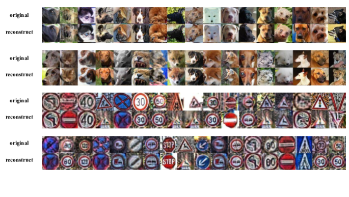
Figure 7 contains more examples of reconstructed input samples by the image translator. To recap, our baselines consist of reconstructed samples instead of original input samples, in order to ensure data distribution consistency compared to the translated samples.

References

- Feng et al. [2023] Chun-Mei Feng, Kai Yu, Yong Liu, Salman Khan, and Wangmeng Zuo. Diverse data augmentation with diffusions for effective test-time prompt tuning. In Proceedings of the IEEE/CVF International Conference on Computer Vision, pages 2704–2714, 2023.
- Gao et al. [2018] Hang Gao, Zheng Shou, Alireza Zareian, Hanwang Zhang, and Shih-Fu Chang. Low-shot learning via covariance-preserving adversarial augmentation networks. Advances in Neural Information Processing Systems, 31, 2018.
- Hariharan and Girshick [2017] Bharath Hariharan and Ross Girshick. Low-shot visual recognition by shrinking and hallucinating features. In Proceedings of the IEEE international conference on computer vision, pages 3018–3027, 2017.
- He et al. [2016] Kaiming He, Xiangyu Zhang, Shaoqing Ren, and Jian Sun. Deep residual learning for image recognition. In Proceedings of the IEEE conference on computer vision and pattern recognition, pages 770–778, 2016.
- Huang and Belongie [2017] Xun Huang and Serge Belongie. Arbitrary style transfer in real-time with adaptive instance normalization. In Proceedings of the IEEE international conference on computer vision, pages 1501–1510, 2017.
- Karras et al. [2019] Tero Karras, Samuli Laine, and Timo Aila. A style-based generator architecture for generative adversarial networks. In Proceedings of the IEEE/CVF conference on computer vision and pattern recognition, pages 4401–4410, 2019.
- Ketcham et al. [1974] David J Ketcham, Roger W Lowe, and J William Weber. Image enhancement techniques for cockpit displays. Hughes Aircraft Co Culver City Ca Display Systems Lab, 1974.
- Kim et al. [2020] Ildoo Kim, Younghoon Kim, and Sungwoong Kim. Learning loss for test-time augmentation. Advances in Neural Information Processing Systems, 33:4163–4174, 2020.
- Kim et al. [2019] Junsik Kim, Tae-Hyun Oh, Seokju Lee, Fei Pan, and In So Kweon. Variational prototyping-encoder: One-shot learning with prototypical images. In Proceedings of the IEEE/CVF Conference on Computer Vision and Pattern Recognition, pages 9462–9470, 2019.
- Kim et al. [2022] Yujin Kim, Jaehoon Oh, Sungnyun Kim, and Se-Young Yun. How to fine-tune models with few samples: Update, data augmentation, and test-time augmentation, 2022.
- Liu et al. [2017] Ming-Yu Liu, Thomas Breuel, and Jan Kautz. Unsupervised image-to-image translation networks. Advances in neural information processing systems, 30, 2017.
- Liu et al. [2019a] Ming-Yu Liu, Xun Huang, Arun Mallya, Tero Karras, Timo Aila, Jaakko Lehtinen, and Jan Kautz. Few-shot unsueprvised image-to-image translation. In arxiv, 2019a.
- Liu et al. [2019b] Ming-Yu Liu, Xun Huang, Arun Mallya, Tero Karras, Timo Aila, Jaakko Lehtinen, and Jan Kautz. Few-shot unsupervised image-to-image translation, 2019b.
- Luo et al. [2021] Qinxuan Luo, Lingfeng Wang, Jingguo Lv, Shiming Xiang, and Chunhong Pan. Few-shot learning via feature hallucination with variational inference. In Proceedings of the IEEE/CVF Winter Conference on Applications of Computer Vision, pages 3963–3972, 2021.
- Mishra et al. [2018] Ashish Mishra, Shiva Krishna Reddy, Anurag Mittal, and Hema A Murthy. A generative model for zero shot learning using conditional variational autoencoders. In Proceedings of the IEEE conference on computer vision and pattern recognition workshops, pages 2188–2196, 2018.
- Oussidi and Elhassouny [2018] Achraf Oussidi and Azeddine Elhassouny. Deep generative models: Survey. In 2018 International conference on intelligent systems and computer vision (ISCV), pages 1–8. IEEE, 2018.
- Park et al. [2019] Taesung Park, Ming-Yu Liu, Ting-Chun Wang, and Jun-Yan Zhu. Semantic image synthesis with spatially-adaptive normalization. In Proceedings of the IEEE/CVF conference on computer vision and pattern recognition, pages 2337–2346, 2019.
- Paszke et al. [2019] Adam Paszke, Sam Gross, Francisco Massa, Adam Lerer, James Bradbury, Gregory Chanan, Trevor Killeen, Zeming Lin, Natalia Gimelshein, Luca Antiga, Alban Desmaison, Andreas Kopf, Edward Yang, Zachary DeVito, Martin Raison, Alykhan Tejani, Sasank Chilamkurthy, Benoit Steiner, Lu Fang, Junjie Bai, and Soumith Chintala. Pytorch: An imperative style, high-performance deep learning library. In Advances in Neural Information Processing Systems 32, pages 8024–8035. Curran Associates, Inc., 2019.
- Ribeiro et al. [2016] Marco Tulio Ribeiro, Sameer Singh, and Carlos Guestrin. Model-agnostic interpretability of machine learning. arXiv preprint arXiv:1606.05386, 2016.
- Rombach et al. [2022] Robin Rombach, Andreas Blattmann, Dominik Lorenz, Patrick Esser, and Björn Ommer. High-resolution image synthesis with latent diffusion models, 2022.
- Russakovsky et al. [2015] Olga Russakovsky, Jia Deng, Hao Su, Jonathan Krause, Sanjeev Satheesh, Sean Ma, Zhiheng Huang, Andrej Karpathy, Aditya Khosla, Michael Bernstein, Alexander C. Berg, and Li Fei-Fei. ImageNet Large Scale Visual Recognition Challenge. International Journal of Computer Vision (IJCV), 115(3):211–252, 2015.
- Saito et al. [2020] Kuniaki Saito, Kate Saenko, and Ming-Yu Liu. Coco-funit: Few-shot unsupervised image translation with a content conditioned style encoder. In Computer Vision–ECCV 2020: 16th European Conference, Glasgow, UK, August 23–28, 2020, Proceedings, Part III 16, pages 382–398. Springer, 2020.
- Schonfeld et al. [2019] Edgar Schonfeld, Sayna Ebrahimi, Samarth Sinha, Trevor Darrell, and Zeynep Akata. Generalized zero-and few-shot learning via aligned variational autoencoders. In Proceedings of the IEEE/CVF conference on computer vision and pattern recognition, pages 8247–8255, 2019.
- Schwartz et al. [2018] Eli Schwartz, Leonid Karlinsky, Joseph Shtok, Sivan Harary, Mattias Marder, Abhishek Kumar, Rogerio Feris, Raja Giryes, and Alex Bronstein. Delta-encoder: an effective sample synthesis method for few-shot object recognition. Advances in neural information processing systems, 31, 2018.
- Snell et al. [2017] Jake Snell, Kevin Swersky, and Richard Zemel. Prototypical networks for few-shot learning. Advances in neural information processing systems, 30, 2017.
- Stallkamp et al. [2012] Johannes Stallkamp, Marc Schlipsing, Jan Salmen, and Christian Igel. Man vs. computer: Benchmarking machine learning algorithms for traffic sign recognition. Neural networks, 32:323–332, 2012.
- van der Maaten and Hinton [2008] Laurens van der Maaten and Geoffrey Hinton. Visualizing data using t-SNE. Journal of Machine Learning Research, 9:2579–2605, 2008.
- Van der Walt et al. [2014] Stefan Van der Walt, Johannes L Schönberger, Juan Nunez-Iglesias, François Boulogne, Joshua D Warner, Neil Yager, Emmanuelle Gouillart, and Tony Yu. scikit-image: image processing in python. PeerJ, 2:e453, 2014.
- Vaswani et al. [2017] Ashish Vaswani, Noam Shazeer, Niki Parmar, Jakob Uszkoreit, Llion Jones, Aidan N. Gomez, Lukasz Kaiser, and Illia Polosukhin. Attention is all you need, 2017.
- Verma et al. [2018] Vinay Kumar Verma, Gundeep Arora, Ashish Mishra, and Piyush Rai. Generalized zero-shot learning via synthesized examples. In Proceedings of the IEEE conference on computer vision and pattern recognition, pages 4281–4289, 2018.
- Vinyals et al. [2016] Oriol Vinyals, Charles Blundell, Timothy Lillicrap, Koray Kavukcuoglu, and Daan Wierstra. Matching networks for one shot learning, 2016.
- Wang et al. [2022] Guotai Wang, Wenqi Li, Michael Aertsen, Jan Deprest, Sebastien Ourselin, and Tom Vercauteren. Test-time augmentation with uncertainty estimation for deep learning-based medical image segmentation. 2022.
- Wang et al. [2017] Kunfeng Wang, Chao Gou, Yanjie Duan, Yilun Lin, Xinhu Zheng, and Fei-Yue Wang. Generative adversarial networks: introduction and outlook. IEEE/CAA Journal of Automatica Sinica, 4(4):588–598, 2017.
- Wang et al. [2018a] Ting-Chun Wang, Ming-Yu Liu, Jun-Yan Zhu, Andrew Tao, Jan Kautz, and Bryan Catanzaro. High-resolution image synthesis and semantic manipulation with conditional gans. In Proceedings of the IEEE conference on computer vision and pattern recognition, pages 8798–8807, 2018a.
- Wang et al. [2020] Yaqing Wang, Quanming Yao, James T Kwok, and Lionel M Ni. Generalizing from a few examples: A survey on few-shot learning. ACM computing surveys (csur), 53(3):1–34, 2020.
- Wang et al. [2018b] Yu-Xiong Wang, Ross Girshick, Martial Hebert, and Bharath Hariharan. Low-shot learning from imaginary data. In Proceedings of the IEEE conference on computer vision and pattern recognition, pages 7278–7286, 2018b.
- Yamada and Matsumi [2021] Keiichi Yamada and Susumu Matsumi. One-shot image learning using test-time augmentation. In Asian Conference on Pattern Recognition, pages 3–16. Springer, 2021.
- Ye et al. [2020] Han-Jia Ye, Hexiang Hu, De-Chuan Zhan, and Fei Sha. Few-shot learning via embedding adaptation with set-to-set functions. In IEEE/CVF Conference on Computer Vision and Pattern Recognition (CVPR), pages 8808–8817, 2020.
- Zhou [2012] Zhi-Hua Zhou. Ensemble methods: foundations and algorithms. CRC press, 2012.
- Zhu et al. [2017] Jun-Yan Zhu, Taesung Park, Phillip Isola, and Alexei A Efros. Unpaired image-to-image translation using cycle-consistent adversarial networks. In Proceedings of the IEEE international conference on computer vision, pages 2223–2232, 2017.
- Zhu et al. [2016] Zhe Zhu, Dun Liang, Songhai Zhang, Xiaolei Huang, Baoli Li, and Shimin Hu. Traffic-sign detection and classification in the wild. In Proceedings of the IEEE conference on computer vision and pattern recognition, pages 2110–2118, 2016.