Towards Better Understanding of Contrastive Sentence Representation Learning: A Unified Paradigm for Gradient

Abstract

Sentence Representation Learning (SRL) is a crucial task in Natural Language Processing (NLP), where contrastive Self-Supervised Learning (SSL) is currently a mainstream approach. However, the reasons behind its remarkable effectiveness remain unclear. Specifically, in other research fields, contrastive SSL shares similarities in both theory and practical performance with non-contrastive SSL (e.g., alignment & uniformity, Barlow Twins, and VICReg). However, in SRL, contrastive SSL outperforms non-contrastive SSL significantly. Therefore, two questions arise: First, what commonalities enable various contrastive losses to achieve superior performance in SRL? Second, how can we make non-contrastive SSL, which is similar to contrastive SSL but ineffective in SRL, effective? To address these questions, we start from the perspective of gradients and discover that four effective contrastive losses can be integrated into a unified paradigm, which depends on three components: the Gradient Dissipation, the Weight, and the Ratio. Then, we conduct an in-depth analysis of the roles these components play in optimization and experimentally demonstrate their significance for model performance. Finally, by adjusting these components, we enable non-contrastive SSL to achieve outstanding performance in SRL.

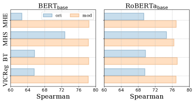
Figure 1: Average Spearman’s correlation on Semantic Textual Similarity tasks for ineffective optimization objectives before (“ori”) and after (“mod”) modifications under different backbones.

1 Introduction

Sentence Representation Learning (SRL) explores how to transform sentences into vectors (or “embeddings”), which contain rich semantic information and are crucial to many downstream tasks in Natural Language Processing (NLP). In the era of Large Language Models (LLMs), SRL also plays an important role in providing the embedding models for Retrieval-Augmented Generation Gao et al. (2023)). The quality of sentence embeddings is usually measured through Transfer tasks (TR) and Semantic Textual Similarity tasks (STS) (Conneau and Kiela, 2018), where transfer tasks can be effectively addressed by pre-trained language models (Devlin et al., 2019), and current research primarily focuses on the performance in STS tasks (Li et al., 2020; Nie et al., 2023).

Contrastive Self-Supervised Learning (SSL) is now prevalent in SRL, which is introduced by Gao et al. (2021) and Yan et al. (2021). It optimizes the representation space by reducing the distance between a sentence (or “anchor”) and semantically similar sentences (or “positive samples”, usually obtained through data augmentation), as well as increasing the distance between the sentence and semantically dissimilar sentences (or “negative samples”, usually obtained through random sampling).

While the mechanisms underlying contrastive SSL can be intuitively understood, its effectiveness in SRL has not been thoroughly explored. Specifically, there are still some conflicts between the existing conclusions in SRL and other areas: (1) Machine learning community has found that contrastive SSL shares theoretical similarities with non-contrastive SSL (e.g. alignment & uniformity (Wang and Isola, 2020), Barlow Twins (Zbontar et al., 2021), and VICReg (Bardes et al., 2022)) (Balestriero and LeCun, 2022; Tao et al., 2022) (2) In Visual Representation Learning (VRL), all these contrastive and non-contrastive SSL methods show comparable performance. However, in SRL, the methods based on contrastive SSL seem to be the only effective ones, outperforming non-contrastive SSL significantly. Even with extensive hyper-parameter selection, various methods in non-contrastive SSL face problems of overfitting Nie et al. (2023) and low performance Klein and Nabi (2022); Xu et al. (2023) in SRL. These inconsistent conclusions imply unique requirements for optimizing SRL have been overlooked in other research areas and have not yet been explored by existing studies in SRL.

In this work, we attempt to identify the key factors that enable contrastive SSL to be effective in SRL. Specifically, we would like to answer two questions: (1) What commonalities enable various contrastive losses to achieve superior performance in SRL? (2) How can we make non-contrastive SSL, which is similar to contrastive SSL but ineffective in SRL, effective? We first analyze the commonalities among four effective losses (Oord et al., 2018; Zhang et al., 2022b; Nie et al., 2023) in SRL from the perspective of gradients. From this analysis, we find that all gradients can be unified into the same paradigm, which is determined by three components: the Gradient Dissipation, the Weight, and the Ratio. By statistically analyzing the values of these three components under different representation space distributions, we propose three conjectures, each corresponding to the role of a component in optimizing the representation space. Subsequently, we construct a baseline model to empirically validate our conjectures. Furthermore, we comprehensively demonstrate the significance of these components to model performance by varying them in the baseline.

After understanding the key factors that enable contrastive losses to be effective, we are able to analyze the reasons behind the poor performance of non-contrastive SSL in SRL from the perspective of three components in the paradigm. We find that these ineffective losses do not perform as well as effective ones across these components. Therefore, by adjusting these components, we manage to make them function and achieve improved model performance in SRL (refer to Figure 1).

Briefly, our main contributions are as follows:

• We propose a unified gradient paradigm for effective losses in SRL, which is controlled by three components: the Gradient Dissipation, the Weight, and the Ratio (Section 2);

• We analyze the roles in optimization for each component theoretically. Further, we propose and validate the conjectures on their effective roles in performing STS tasks (Section 3);

• With the guidance of our analysis results, we modify four optimization objectives in non-contrastive SSL to be effective in SRL by adjusting the three components (Section 4).

2 A Unified Paradigm for Gradient

Objective	Gradient Dissipation	Weight	Ratio
InfoNCE (2018)	$\begin{aligned} 1/(1+\frac{e^{\cos(\theta_{ii^{\prime}})/\tau}}{\sum_{k\neq i}^{N}e^{\cos(\theta_{ik^{\prime}})/\tau}})\end{aligned}$	$\begin{aligned} \frac{e^{\cos(\theta_{ij^{\prime}})/\tau}}{\tau\sum_{k\neq i}^{N}e^{\cos(\theta_{ik^{\prime}})/\tau}}\end{aligned}$	1
ArcCon (2022b)	$\begin{aligned} 1/(1+\frac{e^{\cos(\theta_{ii^{\prime}}+u)/\tau}}{\sum_{k\neq i}^{N}e^{\cos(\theta_{ik^{\prime}})/\tau}})\end{aligned}$	$\begin{aligned} \frac{e^{\cos(\theta_{ij^{\prime}})/\tau}}{\tau\sum_{k\neq i}^{N}e^{\cos(\theta_{ik^{\prime}})/\tau}}\end{aligned}$	$\begin{aligned} \frac{\sin(\theta_{ii^{\prime}}+u)}{\sin(\theta_{ii^{\prime}})}\end{aligned}$
MPT (2023)	$\begin{aligned} \mathbb{I}_{\{\cos(\theta_{ii^{\prime}})-\max\limits_{k\neq i}\cos(\theta_{ik^{\prime}})<m\}}\end{aligned}$	$\begin{aligned} \left\{\begin{aligned} &1,\quad\mathrm{else}\\ &0,\quad j\neq\arg\min_{k\neq i}\theta_{ik^{\prime}}\end{aligned}\right.\end{aligned}$	1
MET (2023)	$\begin{aligned} \mathbb{I}_{\{\min\limits_{k\neq i}\sqrt{2-2\cos(\theta_{ik^{\prime}})}-\sqrt{2-2\cos(\theta_{ii^{\prime}})}<m\}}\end{aligned}$	$\left\{\begin{aligned} &1/\sqrt{2-2\cos(\theta_{ij^{\prime}})},\ \mathrm{else}\\ &0,\quad j\neq\arg\min_{k\neq i}\theta_{ik^{\prime}}\end{aligned}\right.$	$\begin{aligned} \sqrt{\frac{1-\cos(\theta_{ij^{\prime}})}{1-\cos(\theta_{ii^{\prime}})}}\end{aligned}$

Table 1: Three components of four different contrastive losses. We convert the cosine similarity (e.g., $h_{i}^{\top}h_{j}^{\prime}$) and distance (e.g., $\|h_{i}-h_{j}^{\prime}\|_{2}$) into angular form (e.g., $\cos(\theta_{ij^{\prime}})$ and $\sqrt{2-2\cos(\theta_{ij^{\prime}})}$, respectively).

2.1 Preliminary

Given a batch of sentences $\{s_{i}\}_{i=1}^{N}$, we adopt a encoder $f(\cdot)$ to obtain two $l_{2}$-normalized embeddings (i.e., $h_{i}$ and $h_{i}^{\prime}$) for two different augmented views of sentence $s_{i}$. Regarding $h_{i}$ as the anchor, the embedding from the same sentence (i.e., $h_{i}^{\prime}$) is called the positive sample, while the embeddings from the other sentences (i.e., $h_{j}$ and $h_{j}^{\prime},j\neq i$) are called negative samples. Then, what contrastive learning does is to increase the similarity (typically cosine similarity) between the anchor and its positive sample and decrease the similarity between the anchor and its negative samples.

2.2 Gradient Analysis

To understand the optimization mechanism rigorously, we choose four contrastive losses used in recent works and derive the gradient for them. Note that all the loss functions have been proven to be effective in SRL and can obtain competitive performance based on the model architecture of SimCSE Gao et al. (2021).

InfoNCE (Oord et al., 2018) is a widely used contrastive loss introduced to SRL by ConSERT (Yan et al., 2021) and SimCSE (Gao et al., 2021). It can be formed as

$$\mathcal{L}^{\mathrm{info}}_{i}=-\log\frac{e^{h_{i}^{\top}h_{i}^{\prime}/\tau}}{\sum_{j=1}^{N}e^{h_{i}^{\top}h_{j}^{\prime}/\tau}},$$

where $\tau$ is a temperature hyperparameter. The gradient of $\mathcal{L}^{\mathrm{info}}_{i}$ w.r.t $h_{i}$ is

$$\frac{\partial\mathcal{L}^{\mathrm{info}}_{i}}{\partial h_{i}}=\frac{\sum_{j\neq i}^{N}e^{h_{i}^{\top}h_{j}^{\prime}/\tau}(h_{j}^{\prime}-h_{i}^{\prime})}{\tau\sum_{k=1}^{N}e^{h_{i}^{\top}h_{k}^{\prime}/\tau}}.$$ (1)

ArcCon (Zhang et al., 2022b) improves InfoNCE by enhancing the pairwise discriminative power and it can be formed as

$$\mathcal{L}^{\mathrm{arc}}_{i}=-\log\frac{e^{\cos(\theta_{ii^{\prime}}+u)/\tau}}{e^{\cos(\theta_{ii^{\prime}}+u)/\tau}+\sum_{j\neq i}^{N}e^{h_{i}^{\top}h_{j}^{\prime}/\tau}},$$

where $\theta_{ij}=\arccos(h_{i}^{\top}h_{j})$ and $u$ is a hyperparameter. The gradient of $\mathcal{L}^{\mathrm{arc}}_{i}$ w.r.t $h_{i}$ is

$$\frac{\partial\mathcal{L}^{\mathrm{arc}}_{i}}{\partial h_{i}}= \frac{\sum_{j\neq i}^{N}e^{h_{i}^{\top}h_{j}^{\prime}/\tau}(h_{j}^{\prime}-\frac{\sin(\theta_{ii^{\prime}}+u)}{\sin(\theta_{ii^{\prime}})}h_{i}^{\prime})}{\tau(e^{\cos(\theta_{ii^{\prime}}+u)/\tau}+\sum_{k\neq i}^{N}e^{h_{i}^{\top}h_{k}^{\prime}/\tau})}.$$ (2)

MPT and MET (Nie et al., 2023) are two loss functions in the form of triplet loss in SRL, which have the same form:

$$\mathcal{L}^{\mathrm{tri}}_{i}=\max(0,d(h_{i},h_{i}^{\prime})-\max_{j\neq i}d(h_{i},h_{j}^{\prime})+m),$$

where $m$ is a margin hyperparameter and $d:R^{d}\times R^{d}\rightarrow R$ is metric function. Specifically, the only difference among the three loss functions is $d(a,b)$, which is $-a^{T}b$ for MPT and $||a-b||_{2}$ for MET. Similarly, we can obtain their gradient w.r.t $h_{i}$:

$$\frac{\partial\mathcal{L}^{\mathrm{mpt}}_{i}}{\partial h_{i}}=\mathbb{I}\times(h_{j}^{\prime}-h_{i}^{\prime}),$$ (3)

$$\frac{\partial\mathcal{L}^{\mathrm{met}}_{i}}{\partial h_{i}}=\mathbb{I}\times\left(\frac{h_{j}^{\prime}}{\|h_{i}-h_{j}^{\prime}\|_{2}}-\frac{h_{i}^{\prime}}{\|h_{i}-h_{i}^{\prime}\|_{2}}\right),$$

where $j=\mathop{\arg\max}h_{i}^{\top}h_{k}^{\prime}(k\neq i)$ and $\mathbb{I}$ is an indicator function equal to 1 only if $d(h_{i},h_{j}^{\prime})-d(h_{i}.h_{i}^{\prime})<m$ satisfies.

Comparing the above gradient forms, we find that all gradients guide the anchor $h_{i}$ move towards its positive sample $h_{i}^{\prime}$ and away from its negative samples $h_{j}^{\prime}$. It implies that these various forms of loss functions have some commonalities in the perspective of the gradient. After reorganizing the gradient forms, we find that they can all be mapped into a unified paradigm:

$$\frac{\partial\mathcal{L}_{i}}{\partial h_{i}}=\mathrm{GD}(\cdot)\sum_{j\neq i}^{N}\mathrm{W}(\cdot)(h_{j}^{\prime}-\mathrm{R}(\cdot)h_{i}^{\prime}).$$ (4)

There are three components control this paradigm:

• $\mathrm{GD}(i,\{h_{k},h_{k}^{\prime}\}_{k=1}^{N})$ is the Gradient Dissipation term, which overall controls the magnitude of the gradient;

• $\mathrm{W}(i,j,\{h_{k},h_{k}^{\prime}\}_{k=1}^{N})$ is the Weight term, which controls the magnitude of the contribution of negative samples to the gradient;

• $\mathrm{R}(i,j,\{h_{k},h_{k}^{\prime}\}_{k=1}^{N})$ is the Ratio term, which controls the magnitude of the contribution of positive samples to the gradient;

Table 1 shows the specific form of three components in each loss, which all have been converted into the angular form for subsequent analysis.

3 Role of Each Component

3.1 Theoretical Analysis

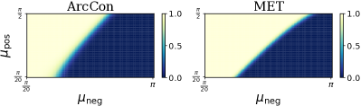
Figure 2: Average values of gradient dissipation term under different $\mu_{\mathrm{pos}}$-$\mu_{\mathrm{neg}}$ pairs for ArcCon and MET. Appendix B shows the results for InfoNCE and MPT.

Although the above losses are unified into the same paradigm, the specific forms of the three components in different loss functions are various. Therefore, we first demonstrate that their roles are consistent despite their varied forms. To validate this, we record the trends of each component with the anchor-positive angle $\theta_{ii^{\prime}}$ and anchor-negative angle $\theta_{ij^{\prime}}$ and confirm whether there are consistent trends under different forms.

Specifically, we assume that $\theta_{ii^{\prime}}$ and $\theta_{ij^{\prime}}$ follow normal distribution $\mathcal{N}(\mu_{\mathrm{pos}},\sigma_{\mathrm{pos}}^{2})$ and $\mathcal{N}(\mu_{\mathrm{neg}},\sigma_{\mathrm{neg}}^{2})$, respectively. Based on experimental evidence, we draw $\mu_{\mathrm{pos}}$ from $[\frac{\pi}{20},\frac{\pi}{2}]$, and $\mu_{\mathrm{neg}}$ from $[\frac{\pi}{20},\pi]$, with $\sigma_{\mathrm{pos}}$ fixed at 0.05 and $\sigma_{\mathrm{neg}}$ fixed at 0.10. After validating the consistency among different forms, we propose intuitive conjectures regarding the roles played by each component.

3.1.1 Gradient Dissipation

To study the role of the gradient dissipation term, we experiment with three steps: (1) For both $\mu_{\mathrm{pos}}$ and $\mu_{\mathrm{neg}}$, we divide their intervals equally into 100 parts to obtain 10,000 $\mu_{\mathrm{pos}}$-$\mu_{\mathrm{neg}}$ pairs, covering all situations of the entire optimization process; (2) For each $\mu_{\mathrm{pos}}$-$\mu_{\mathrm{neg}}$ pair, we sample 1,000 batches, each comprising 1 sampled from $\theta_{ii^{\prime}}$ and 127 sampled from $\theta_{ij^{\prime}}$; (3) The average value of the gradient dissipation term is calculated across these batches. The results are plotted in Figure 2 with heatmaps.

There are two forms of gradient dissipation: one is implemented through fraction functions (including InfoNCE and ArcCon), and the other is implemented through indicator functions (including MPT and MET). The results in Figure 2 show that both the two forms of the gradient dissipation term exhibit a similar pattern: when $\mu_{\mathrm{pos}}$ and $\mu_{\mathrm{neg}}$ are close, the value is 1; when $\mu_{\mathrm{neg}}$ is larger than $\mu_{\mathrm{pos}}$ to some extent, the value rapidly decreases to 0. Intuitively, this term avoids a great distance gap between the anchor-positive and the anchor-negative pairs. Recall that the semantic similarity is scored on a scale from 0 to 5 in traditional STS tasks, rather than being binary classified as similar or dissimilar. Such a great gap may deteriorate the performance of sentence embeddings in STS tasks. Therefore, we propose

Conjecture 1.

The effective gradient dissipation term ensures that the distance gap between $\mu_{\mathrm{neg}}$ and $\mu_{\mathrm{pos}}$ remains smaller than the situation trained without gradient dissipation.

3.1.2 Weight

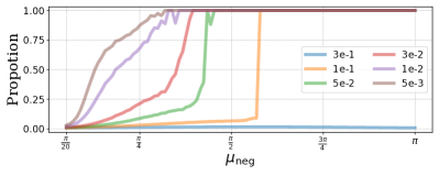
Figure 3: Variations in the average portion of the hardest negative samples in the weight across different $\mu_{\mathrm{neg}}$, under different temperatures $\tau$.

To study the role of the weight term, we also experiment with three steps: (1) For $\mu_{\mathrm{neg}}$, we divide its intervals equally into 100 parts, while for $\mu_{\mathrm{pos}}$, we fixed its value to $\frac{\pi}{6}$. Then we can obtain 100 $\mu_{\mathrm{pos}}$-$\mu_{\mathrm{neg}}$ pairs to analyze the relative contribution among the negative samples; (2) For each $\mu_{\mathrm{pos}}$-$\mu_{\mathrm{neg}}$ pair, we sample 1000 batches, each comprising 1 sampled from $\theta_{ii^{\prime}}$ and 127 sampled from $\theta_{ij^{\prime}}$; (3) The average proportion of the weight for the hardest negative sample (i.e., the one with the highest cosine similarity to the anchor) is calculated. The results calculated under different temperatures are plotted in Figure 3.

There are two forms of weight: one is implemented through the exponential function (including InfoNCE and ArcCon), and the other is implemented through the piecewise function (including MPT and MET). For the piecewise-form weight, the value is non-zero if and only if the negative sample is the hardest. Therefore, to prove the consistency between these two forms, it is only need to examine the proportion of the hardest negative samples in the exponential-form weight. The results show that the exponential-form weight also becomes focused solely on the hardest negative examples during the training process, similar to the piecewise-form weight. Therefore, we propose

Conjecture 2.

The effective weight term ensures that the hardest negative sample occupies a dominant position in the gradient compared to other negative samples.

3.1.3 Ratio

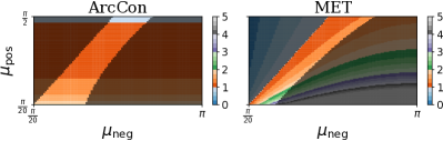
Figure 4: Average values of three dynamic ratio terms, The shaded areas indicate that these $\mu_{\mathrm{pos}}$-$\mu_{\mathrm{neg}}$ pairs do not occur in the actual optimization process, where the lower part is due to gradient dissipation, and the upper part is because there is always $\mu_{\mathrm{pos}}<\mu_{\mathrm{neg}}$.

The ratio term can be categorized into two types: One is the static ratio (including InfoNCE and MPT), keeping the value of 1; The other is the dynamic ratio (including ArcCon and MET), with values dependent on $\theta_{ii^{\prime}}$ and $\theta_{ij^{\prime}}$. To investigate the value range of the dynamic ratio, we follow the first two steps in Section 3.1.1 and calculate the values of different dynamic ratio terms. The results are plotted in Figure 4. As shown in the figure, the dynamic ratio varies significantly. However, when considering the impact of gradient dissipation and the fact that $\mu_{\mathrm{pos}}$ is typically smaller than $\mu_{\mathrm{neg}}$, it can be found that the values of the dynamic ratio mostly fall between 1 and 2.

There exists an interesting phenomenon where sentence embeddings trained with ArcCon outperform those trained with InfoNCE, and MET does the same for MPT (Refer to Table 3). However, as observed in previous analyses, the gradient dissipation term and the weight term of these losses are essentially consistent. Therefore, we believe that it is precisely because ArcCon and MET can achieve larger ratios during the training process that these losses exhibit better performance, which can be explained through the following lemma.

Lemma 1.

For an anchor $h_{i}$ and its positive sample $h_{i}^{\prime}$ and negative sample $h_{j}^{\prime}$, assume the angle between the plane $Oh_{i}h_{i}^{\prime}$ and the plane $Oh_{i}h_{j}^{\prime}$ is $\alpha$. When $h_{i}$ moves along the optimization direction $\lambda(rh_{i}^{\prime}-h_{j}^{\prime})$, $r$ must satisfy

$$r>\frac{1}{\lambda}+\frac{\sin\theta_{ij^{\prime}}\cos\alpha}{\sin\theta_{ii^{\prime}}}-\sqrt{\frac{1}{\lambda^{2}}-\frac{\sin^{2}\theta_{ij^{\prime}}\sin^{2}\alpha}{\sin^{2}\theta_{ii^{\prime}}}}.$$

to ensure the distance from $h_{i}$ to $h_{i}^{\prime}$ becomes closer after the optimization step.

The larger ratios in ArcCon and MET enable them to meet the condition in more situations, thereby exhibiting better performance. We propose

Conjecture 3.

The effective ratio term can meet the condition in Lemma 1 more frequently, and ensure that the distance from the anchor to the positive sample is closer after optimization than that before optimization.

3.2 Empirical Study

To validate the conjectures in Section 3.1 and further investigate the impact of each component on the model performance, this section conducts experiments based on

$$\mathcal{L}_{i}=\mathrm{GD}(\cdot)\sum_{j\neq i}^{N}\mathrm{W}(\cdot)\left(h_{i}^{\top}h_{j}^{\prime}-\mathrm{R}(\cdot)h_{i}^{\top}h_{i}^{\prime}\right),$$ (5)

where $\mathrm{GD}(\cdot)$, $\mathrm{W}(\cdot)$, and $\mathrm{R}(\cdot)$ do not require gradient. It can be easily verified that the gradient of $\mathcal{L}_{i}$ w.r.t $h_{i}$ is the paradigm in Equation 4. We select $\mathrm{GD}(\cdot)=\mathbb{I}_{\{h_{i}^{\top}h_{i}^{\prime}-\max_{k\neq i}^{N}h_{i}^{\top}h_{k}^{\prime}<m\}}$, $\mathrm{W}(\cdot)=\frac{e^{h_{i}^{\top}h_{j}^{\prime}/\tau}}{\sum_{k\neq i}^{N}e^{h_{i}^{\top}h_{k}^{\prime}/\tau}}$, $\mathrm{R}(\cdot)=r$, and $m=0.3,\tau=0.05,r=1$ as baseline. We adopt BERT_base (Devlin et al., 2019) as backbone and utilize commonly used unsupervised datasets (Gao et al., 2021) as training data. In validating conjectures, we divide the training data into two parts, where 90% is used for training and 10% is held out for statistical analysis. In investigating the impact of each component on performance, we vary each component in the baseline and train with all data, with Spearman’s correlation on the STS-B (Cer et al., 2017) validation set as the performance metric.

3.2.1 Validation of Conjecture 1

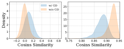
Figure 5: Distribution of cosine similarity for anchor-negative pairs (left) and anchor-positive pairs (right).

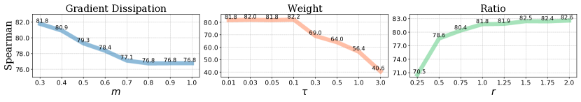
Figure 6: Spearman’s correlation on the STS-B validation set when changing the three components in the baseline.

To verify Conjecture 1, we compare the distribution of $\theta_{ii^{\prime}}$ and $\theta_{ij^{\prime}}$ in sentence embeddings obtained from baseline training and from training without gradient dissipation (i.e., setting $\mathrm{GD}(\cdot)=1$). The results, presented in Figure 5, indicate that the distribution of $\theta_{ii^{\prime}}$ is closer to that of $\theta_{ij^{\prime}}$ when gradient dissipation is applied, compared to the scenario without it, therefore validating the conjecture.

To investigate the impact of the gradient dissipation term on performance, we vary $m$ in $\mathrm{GD}(\cdot)$ from 0.3 to 1 and plot the corresponding performance changes in the first graph of Figure 6. An increase in $m$ implies a weakening effect, and the model performance decreasing as $m$ increases proves the importance of effective gradient dissipation term for model performance.

3.2.2 Validation of Conjecture 2

Figure 7: Average portion of the hardest negative samples in the weight under different temperatures $\tau$, measured on the original BERT model (left) and the BERT model fine-tuned with the baseline loss (right).

To verify Conjecture 2, we calculated the average proportion of the hardest negative samples in the exponential-form weight under different temperature $\tau$, with results presented in Figure 7. In the original BERT, since embeddings are confined within a smaller space (Li et al., 2020), a very small $\tau$ is required to allow the hardest negative samples to occupy a higher proportion. However, in models trained with the baseline, the spatial range of embeddings increases, enabling a commonly used setting ($\tau=0.05$) to also allow the hardest negative samples to dominate the optimization direction. These findings validate the conjecture.

To investigate the impact of the weight term on performance, we vary $\tau$ in $\mathrm{W}(\cdot)$ from 0.01 to 3.0 and plot the corresponding performance changes in the second graph of Figure 6. An increase in $\tau$ means the overall proportion of the hardest negative samples in the gradient decreases. When $\tau$ is increased to 0.3, the proportion begins to sharply decline (refer to Figures 3 and 7), at which point there is also a sharp drop in model performance. This demonstrates the necessity of an effective weight term for model performance.

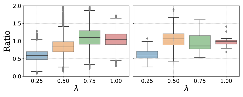
(a) Distribution of the minimum ratio that satisfies the condition under different $\lambda$ for the original BERT model (left) and the BERT model fine-tuned with the baseline loss (right).

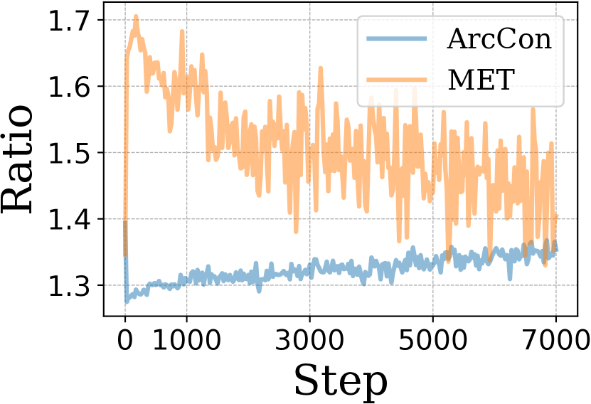
(b) Variations in the dynamic ratios in ArcCon and MET across training steps.

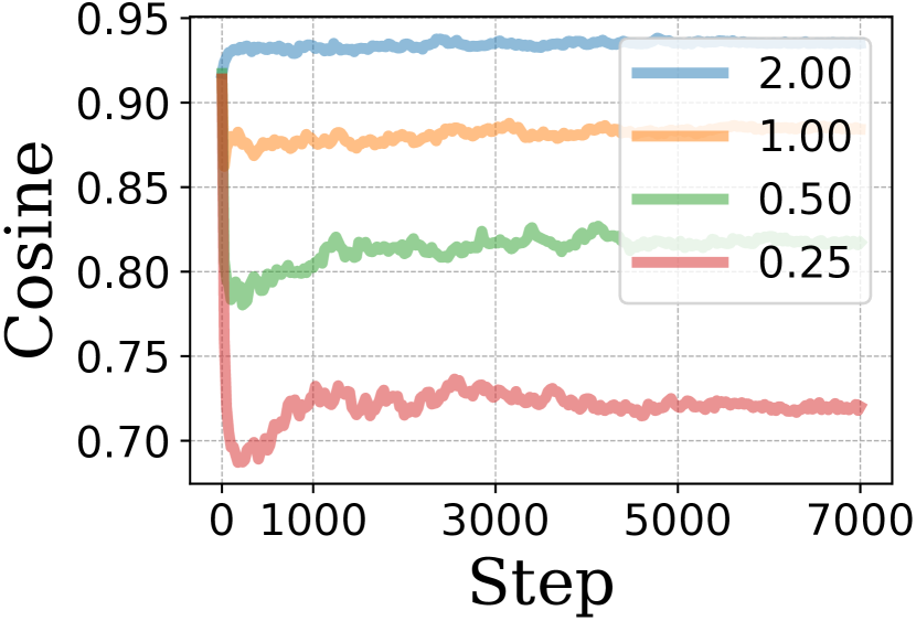
(c) Variations in average cosine similarity across training steps for anchor-positive pairs.

Figure 8: Results for validating Conjecture 3.

3.2.3 Validation of Conjecture 3

To verify Conjecture 3, we first record the distribution of the minimum values required to meet the conditions in Lemma 1 (presented in Figure 8(a)). The results show that, across different models and values of $\lambda$, a ratio greater than 1 consistently meets more conditions. Then, we record the values of three dynamic ratios during the training process (presented in Figure 8(b)). The results show that ArcCon and MET maintain a ratio greater than 1 throughout the training process, thus better fulfilling the lemma’s conditions. Finally, we record the average cosine similarity between the anchor and positive sample during the training process under different ratios (presented in Figure 8(c)). The results show that a larger ratio can indeed result in a closer anchor-positive distance. Together, the above results validate the conjecture.

To investigate the impact of the ratio term on performance, we vary $r$ in $\mathrm{R}(\cdot)$ from 0.25 to 2.0 and plot the corresponding performance changes in the third graph of Figure 6. An increase in $r$ means the conditions in Lemma 1 can be met more frequently, and the model performance improving as $r$ increases proves the significance of an effective ratio term for model performance.

4 Modification to Ineffective Losses

After understanding the properties that the gradients of the effective losses in SRL should possess, we can make some ineffective optimization objectives in non-contrastive SSL effective by adjusting their gradients.

Alignment & Uniformity (Wang and Isola, 2020) are two metrics used to assess the performance of the representation space, yet directly using them as optimization objectives results in poor performance. Alignment can be represented as

$$\mathcal{L}^{\mathrm{a}}=\frac{1}{N}\sum_{i=1}^{N}\|h_{i}-h_{i}^{\prime}\|_{2}^{2},$$

and uniformity can be represented in many forms (Liu et al., 2021), one of which is the Minimum Hyperspherical Energy (MHE)

$$\mathcal{L}^{\mathrm{u,MHE}}=\log\frac{2}{N(N-1)}\sum_{1\leq k<l\leq N}e^{-\|h_{k}-h_{l}\|_{2}^{2}},$$

and another is the Maximum Hyperspherical Separation (MHS)

$$\mathcal{L}^{\mathrm{u,MHS}}_{i}=-\min_{j\neq i}\|h_{i}-h_{j}\|_{2}.$$

Another two widely used optimization objectives in non-contrastive SSL are Barlow Twins (2021)

$$\mathcal{L}^{\mathrm{B}}=\sum_{k=1}^{D}(C_{kk}^{\mathrm{B}}-1)^{2}+\nu^{\mathrm{B}}\sum_{k\neq l}^{D}(C_{kl}^{\mathrm{B}})^{2},$$

where $C^{\mathrm{B}}=\frac{1}{N}\sum_{i=1}^{N}h_{i}h_{i}^{\prime\top}$, and VICReg (2022):

$$\mathcal{L}^{\mathrm{V}}=\mathcal{L}^{\mathrm{a}} +\nu^{\mathrm{V,1}}\left(v(\{h_{i}\}_{i=1}^{N})+v(\{h_{i}^{\prime}\}_{i=1}^{N})\right)$$

$$+\nu^{\mathrm{V,2}}\left(c(\{h_{i}\}_{i=1}^{N})+c(\{h_{i}^{\prime}\}_{i=1}^{N})\right),$$

$$v(\{h_{i}\}_{i=1}^{N} )=\frac{1}{D}\sum_{k\neq l}^{D}(C^{\mathrm{V}}(\{h_{i}\}_{i=1}^{N})_{kl})^{2},$$

$$c(\{h_{i}\}_{i=1}^{N} )=\frac{1}{D}\sum_{k=1}^{D}\max\left(0,\gamma-\sigma(\{h_{i}\}_{i=1}^{N})_{k}\right),$$

where $C^{\mathrm{V}}(\{h_{i}\}_{i=1}^{N})=\frac{1}{N-1}\sum\limits_{i=1}^{N}(h_{i}-\bar{h}_{i})(h_{i}-\bar{h}_{i})^{\top}$, and $\sigma(\cdot)$ is the sample standard deviation. They are both popular in Visual Representation Learning, yet their performances are relatively poor when applied to SRL.

The gradient w.r.t $h_{i}$ for alignment and uniformity ($\mathcal{L}^{\mathrm{a}}+\nu^{\mathrm{u}}\mathcal{L}^{\mathrm{u,MHE}}$ and $\mathcal{L}^{\mathrm{a}}+\nu^{\mathrm{u}}\mathcal{L}^{\mathrm{u,MHS}}_{i}$) and non-contrastive SSL ($\mathcal{L}^{\mathrm{B}}$ and $\mathcal{L}^{\mathrm{V}}$) can also be mapped into the paradigm. We present the results in the upper part of Table 2, where the gradient for $\mathcal{L}^{\mathrm{B}}$ and $\mathcal{L}^{\mathrm{V}}$ is derived by Tao et al. (2022).

	$\mathcal{L}^{\mathrm{a}}+\nu^{\mathrm{u}}\mathcal{L}^{\mathrm{u,MHE}}$	$\mathcal{L}^{\mathrm{a}}+\nu^{\mathrm{u}}\mathcal{L}^{\mathrm{u,MHS}}_{i}$	$\mathcal{L}^{\mathrm{B}}$	$\mathcal{L}^{\mathrm{V}}$
Gradient Dissipation	1
Weight	$\begin{aligned} {\color[rgb]{1,0.6,0.6}\frac{2\nu^{\mathrm{u}}e^{2h_{i}^{\top}h_{j}}}{\sum_{1\leq k<l\leq N}e^{2h_{k}^{\top}h_{l}}}}\end{aligned}$	${\left\{\begin{aligned} &\nu^{\mathrm{u}}/\|h_{i}-h_{j}\|_{2},\ \mathrm{else}\\ &0,j\neq\arg\max_{k\neq i}h_{i}^{\top}h_{k}\end{aligned}\right.}$	$\begin{aligned} {\color[rgb]{1,0.6,0.6}\frac{2\nu^{\mathrm{B}}h_{i}^{\prime\top}h_{j}^{\prime}}{N^{2}}}\end{aligned}$	$\begin{aligned} {\color[rgb]{1,0.6,0.6}\frac{4\nu^{\mathrm{V,1}}h_{i}^{\top}h_{j}}{D(N-1)^{2}}}\end{aligned}$
Ratio	$\begin{aligned} {\color[rgb]{1,0.6,0.6}\frac{\sum_{1\leq k<l\leq N}e^{2h_{k}^{\top}h_{l}}}{\nu^{\mathrm{u}}N\sum_{k\neq i}^{N}e^{2h_{i}^{\top}h_{k}}}}\end{aligned}$	$\begin{aligned} {\color[rgb]{1,0.6,0.6}\frac{2\|h_{i}-h_{j}\|_{2}}{\nu^{\mathrm{u}}N}}\end{aligned}$	$\begin{aligned} {\color[rgb]{1,0.6,0.6}\frac{N(I-(1-\nu^{\mathrm{B}})W_{\mathrm{diag}})}{\nu^{\mathrm{B}}\sum_{k\neq i}^{N}h_{i}^{\prime\top}h_{k}^{\prime}}}\end{aligned}$	$\begin{aligned} {\color[rgb]{1,0.6,0.6}\frac{D(N-1)^{2}N^{-1}}{2\nu^{\mathrm{V,1}}\sum_{k\neq i}^{N}h_{i}^{\top}h_{k}}}\end{aligned}$
	$\mathcal{L}^{\mathrm{mMHE}}_{i}$	$\mathcal{L}^{\mathrm{mMHS}}_{i}$	$\mathcal{L}^{\mathrm{mB}}_{i}$	$\mathcal{L}^{\mathrm{mV}}_{i}$
Gradient Dissipation	$\mathbb{I}_{\{h_{i}^{\top}h_{i}^{\prime}-\max_{k\neq i}^{N}h_{i}^{\top}h_{k}^{\prime}<m\}}$
Weight	$\begin{aligned} \frac{e^{h_{i}^{\top}h_{j}/\tau}}{\tau\sum_{1\leq k<l\leq N}e^{h_{k}^{\top}h_{l}/\tau}}\end{aligned}$	${\left\{\begin{aligned} &1/\|h_{i}-h_{j}\|_{2},\ \mathrm{else}\\ &0,j\neq\arg\max_{k\neq i}h_{i}^{\top}h_{k}\end{aligned}\right.}$	$\begin{aligned} \frac{e^{h_{i}^{\prime\top}h_{j}^{\prime}/\tau}}{\sum_{k\neq l}^{N}e^{h_{k}^{\prime\top}h_{l}^{\prime}/\tau}}\end{aligned}$	$\begin{aligned} \frac{e^{h_{i}^{\top}h_{j}/\tau}}{\sum_{k\neq l}^{N}e^{h_{k}^{\top}h_{l}/\tau}}\end{aligned}$
Ratio	$r$

Table 2: Three components of the ineffective optimization objectives before and after modifications.

Components in the paradigm of ineffective losses do not perform in the same manner as those of effective losses. For gradient dissipation terms, since their values are 1 in all ineffective losses, it implies that they have no effect. For weight terms, except for MHS, other losses cannot ensure that the hardest negative samples dominate in the gradient. For ratio terms, since they are dynamic and cannot guarantee an effective value throughout the optimization process, it is better to adopt a static ratio. Therefore, we attempt to make these losses effective by adjusting these terms, with the results presented in the lower part of Table 2.

We take Barlow Twins as an example to introduce the modification method. For the specific modification process of other optimization objectives, please refer to Appendix E. Based on gradients, the optimization objective of Barlow Twins is equivalent to

$$\mathcal{L}^{\mathrm{eB}}_{i}=-h_{i}^{\top}w_{\mathrm{p},i}^{\mathrm{B}}h_{i}^{\prime}+\nu^{\mathrm{B}}\sum_{j\neq i}^{N}h_{i}^{\top}w_{\mathrm{n},ij}^{\mathrm{B}}h_{j},$$

where $w_{\mathrm{p},i}^{\mathrm{B}}=\frac{2(I-(1-\lambda)W_{\mathrm{diag}})}{N},w_{\mathrm{n},ij}^{\mathrm{B}}=\frac{2h_{i}^{\prime\top}h_{j}^{\prime}I}{N^{2}}$, and both of them do not require gradient. To adjust the gradient dissipation term, we stop the gradient of anchor $h_{i}$ that does not meet the condition ($h_{i}^{\top}h_{i}^{\prime}-\max_{k\neq i}^{N}h_{i}^{\top}h_{k}^{\prime}<m$), which is equivalent to multiplying the loss by the indicator function

$$d_{i}=\mathbb{I}_{\{h_{i}^{\top}h_{i}^{\prime}-\max_{k\neq i}^{N}h_{i}^{\top}h_{k}^{\prime}<m\}}.$$

To adjust the weight term, we first set $\nu^{\mathrm{B}}=1$. Then, we modify $w_{\mathrm{n},ij}^{\mathrm{B}}$ to an exponential form:

$$w_{\mathrm{n},ij}^{\mathrm{mB}}=\frac{e^{h_{i}^{\prime\top}h_{j}^{\prime}/\tau}}{\sum_{k\neq l}e^{h_{k}^{\prime\top}h_{l}^{\prime}/\tau}}.$$

To adjust the ratio term, we set the loss to have a static ratio $r$, by modifying $w_{\mathrm{p},i}^{\mathrm{B}}$ to

$$w_{\mathrm{p},i}^{\mathrm{mB}}=\sum_{j\neq i}^{N}w_{\mathrm{n},ij}^{\mathrm{mB}}=\frac{r\sum_{j\neq i}^{N}e^{h_{i}^{\prime\top}h_{j}^{\prime}/\tau}}{\sum_{k\neq l}e^{h_{k}^{\prime\top}h_{l}^{\prime}/\tau}},$$

which do not require gradients. Finally, the modified Barlow Twins can be represented as

$$\mathcal{L}_{i}^{\mathrm{mB}}=d_{i}(-h_{i}^{\top}w_{\mathrm{p},i}^{\mathrm{mB}}h_{i}^{\prime}+\sum_{j\neq i}^{N}h_{i}^{\top}w_{\mathrm{n},ij}^{\mathrm{mB}}h_{j}).$$ (6)

The performance of all modified optimization objectives is presented in Table 3, where it can be observed that they all exhibit performance comparable to that of effective contrastive losses.

Type	BERTbase		RoBERTabase
	STS.Avg	TR.Avg	STS.Avg	TR.Avg
Pretrained	56.70	85.34	56.57	83.20
$\mathcal{L}_{i}^{\mathrm{info}}$	76.25	85.81	76.57	84.84
$\mathcal{L}_{i}^{\mathrm{arc}}$	77.25	86.08	76.60	86.71
$\mathcal{L}_{i}^{\mathrm{mpt}}$	77.25	87.56	76.42	85.10
$\mathcal{L}_{i}^{\mathrm{met}}$	78.38	87.94	77.38	85.74
$\mathcal{L}_{i}^{\mathrm{mMHE}}$	$\underset{{\color[rgb]{0,0.7,0}+15.78}}{78.40}$	$\underset{{\color[rgb]{0,0.7,0}+\ 0.72}}{85.07}$	$\underset{{\color[rgb]{0,0.7,0}+\ 7.61}}{76.91}$	$\underset{{\color[rgb]{0,0.7,0}+\ 1.36}}{86,28}$
$\mathcal{L}_{i}^{\mathrm{mMHS}}$	$\underset{{\color[rgb]{0,0.7,0}+\ 5.54}}{78.27}$	$\underset{{\color[rgb]{1,0.55,0.55}-\ 0.46}}{85.42}$	$\underset{{\color[rgb]{0,0.7,0}+\ 1.75}}{76.37}$	$\underset{{\color[rgb]{1,0.55,0.55}-\ 0.53}}{86.17}$
$\mathcal{L}_{i}^{\mathrm{mB}}$	$\underset{{\color[rgb]{0,0.7,0}+12.74}}{78.34}$	$\underset{{\color[rgb]{0,0.7,0}+\ 0.34}}{85.28}$	$\underset{{\color[rgb]{0,0.7,0}+\ 7.64}}{77.15}$	$\underset{{\color[rgb]{0,0.7,0}+\ 1.15}}{85.98}$
$\mathcal{L}_{i}^{\mathrm{mV}}$	$\underset{{\color[rgb]{0,0.7,0}+12.71}}{78.24}$	$\underset{{\color[rgb]{0,0.7,0}+\ 0.40}}{85.40}$	$\underset{{\color[rgb]{0,0.7,0}+\ 7.32}}{76.87}$	$\underset{{\color[rgb]{0,0.7,0}+\ 1.14}}{86.11}$

Table 3: Performance on SentEval Benchmark (Conneau and Kiela, 2018) of the four contrastive losses, whose results are from their original paper, and the modified optimization objectives, whose results are the average value obtained from three runs. The values underneath indicate improvements compared to before modification. “STS.Avg” represents the average of Spearman’s correlation on seven STS tasks, and “TR.Avg” represents the average accuracy on seven transfer tasks.

5 Related Work

Contrastive Sentence Representation Learning is initially investigated by Gao et al. (2021) and Yan et al. (2021), followed by numerous efforts (2022a; 2022b; 2022; 2023) that enhance the method’s performance on STS tasks. Beyond these performance-focused studies, Nie et al. (2023) explores the reasons for the success of contrastive SRL, identifying the significance of gradient dissipation in optimization. The distinction of our work lies in further identifying other critical factors and making previously ineffective losses effective.

Similarities between Contrastive and Non-contrastive Self-Supervised Learning are explored in numerous works (2022b; 2023) in Computer Vision (CV). Zhang et al. (2022b) study the similarities between the two methods from the perspective of spectral embedding. Garrido et al. (2023) point out that under certain assumptions, the two methods are algebraically equivalent. Our work makes non-contrastive SSL effective in SRL, revealing that similar parallels also exist in NLP.

Gradients of Self-Supervised Learning are investigated in CV by Tao et al. (2022), which is similar to our methods. The distinction of our work lies in that we work in the field of NLP, and that we explore the impact of different gradient components on optimizing the representation space.

6 Conclusion

In this paper, we propose a unified gradient paradigm for four different optimization objectives in SRL, which is determined by three components: the gradient dissipation, the weight, and the ratio. We uncover the roles these components play in optimization and demonstrate their significance to model performance. Based on these insights, we succeed in making ineffective losses effective in SRL. Our work advances the understanding of why contrastive SSL can be effective in SRL and guides the future design of new optimization objectives.

Limitations

First, our work currently focuses only on the impact of optimization objectives on model performance. This means that the results of this study cannot be applied to analyze the impact of model architecture on model performance. Secondly, modifying the gradient-equivalent form of optimization objectives results in significant differences in the form of optimization objectives before and after modification. To ensure consistency in form, one should make modifications based on observations and experience (see examples in Appendix E).

Appendix A Experiment Details

A.1 Distribution of Representation Space

In analyzing the role that each component plays in optimizing the representation space (Section 3.1), we assume that $\theta_{ii^{\prime}}$ and $\theta_{ij^{\prime}}$ follow normal distributions $\mathcal{N}(\mu_{\mathrm{pos}},\sigma^{2}_{\mathrm{pos}})$ and $\mathcal{N}(\mu_{\mathrm{neg}},\sigma^{2}_{\mathrm{neg}})$, respectively. These assumptions are consistent with the phenomena observed in subsequent experiments (Section 3.2). Specifically, Figure 5 demonstrates that in the representation space, the distributions of $\theta_{ii^{\prime}}$ and $\theta_{ij^{\prime}}$ closely approximate normal distributions, and the $\theta_{ii^{\prime}}$ distribution in Figure 8(c) is within the range of our assumptions. Furthermore, we estimate $\mu_{\mathrm{pos}}$, $\mu_{\mathrm{neg}}$, $\sigma_{\mathrm{pos}}$, and $\sigma_{\mathrm{neg}}$ during trained with the baseline. The results are presented in Figure 9. From these results, it is evident that our assumed ranges for $\mu_{\mathrm{pos}}$ ($[\frac{\pi}{20},\frac{\pi}{2}]$) and $\mu_{\mathrm{neg}}$ ($[\frac{\pi}{20},\pi]$) adequately cover the actual scenarios that may occur. Furthermore, the values of $\sigma_{\mathrm{pos}}$ and $\sigma_{\mathrm{neg}}$ (0.05 and 0.10, respectively) are also close to the practical observations.

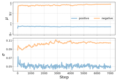
Figure 9: Variations of estimated $\mu_{\mathrm{pos}}$, $\mu_{\mathrm{neg}}$, $\sigma_{\mathrm{pos}}$, and $\sigma_{\mathrm{neg}}$ across training steps when trained with baseline.

A.2 Details of the Empirical Study

In validating the conjectures, we randomly hold out 10% of the data for analyzing the representation space. To obtain results in Figure 5 and Figure 8(c), we directly use the held-out data, and Figure 5 is plotted through Kernel Density Estimation (KDE). To obtain the results in Figure 7, Figure 8(a), and Figure 8(b), we split the held-out data into batches with size $N=128$ and calculate the corresponding values within each batch.

A.3 Training Details

Our implementation of training the representation space is based on SimCSE (Gao et al., 2021), which is currently widely used in research. Our experiments are conducted using Python3.9.13 and Pytorch1.12.1 on a single 32G NVIDIA V100 GPU.

Following Gao et al. (2021), we obtain sentence embeddings from the “[CLS]” token and apply an MLP layer solely during training. The embeddings are trained with 1,000,000 sentences from Wikipedia, which are also collected by Gao et al. (2021), for one epoch. Note that, in validating the conjectures, we randomly hold out 10% of the data for analysis and only use 90% for training.

A.4 Parameter Setting

For experiments in Section 3.2, all experiments are conducted with BERT_base as the backbone and batch size = 128, learning rate = 1e-5.

For the modified losses in Section 4, we first perform a grid search on batch size $\in$ {64, 128, 256, 512}, learning rate $\in$ {5e-6, 1e-5, 3e-5, 5e-5} with $m=0.30$, $\tau=$ 5e-2, and $r=1$. Then, based on the best combination of batch size and learning rate from the first grid search, we perform the second grid search on $m\in$ {0.27, 0.30, 0.33, 0.37}, $\tau\in$ {1e-2, 3e-2, 5e-2}, and $r\in$ {1.00, 1.25, 1.50, 1.75, 2.00}. The results are presented in Table 4 and Table 5.

	bs	lr	$m$	$\tau$	$r$
$\mathcal{L}^{\mathrm{mMHE}}_{i}$	128	1e-5	0.30	5e-2	1.75
$\mathcal{L}^{\mathrm{mMHS}}_{i}$	128	1e-5	0.30	-	1.75
$\mathcal{L}^{\mathrm{mB}}_{i}$	128	1e-5	0.30	5e-2	1.50
$\mathcal{L}^{\mathrm{mV}}_{i}$	128	1e-5	0.30	5e-2	1.50

Table 4: The hyperparameters used to to obtain the results of modified losses in Table 3 when using BERT_base (Devlin et al., 2019) as the backbone.

	bs	lr	$m$	$\tau$	$r$
$\mathcal{L}^{\mathrm{mMHE}}_{i}$	512	1e-5	0.30	5e-2	1.25
$\mathcal{L}^{\mathrm{mMHS}}_{i}$	512	1e-5	0.27	-	1.00
$\mathcal{L}^{\mathrm{mB}}_{i}$	512	1e-5	0.37	5e-2	1.25
$\mathcal{L}^{\mathrm{mV}}_{i}$	512	1e-5	0.37	5e-2	1.25

Table 5: The hyperparameters used to to obtain the results of modified losses in Table 3 when using RoBERTa_base Liu et al. (2019) as the backbone.

A.5 Evaluation Protocol

In Section 3.2 and Section 4, we adopt a widely used evaluation protocol, SentEval toolkit (Conneau and Kiela, 2018), to evaluate the performance of SRL. SentEval includes two types of tasks: the Semantic Textual Similarity (STS) tasks and the Transfer tasks (TR). The STS task quantifies the semantic similarity between two sentences with a score ranging from 0 to 5 and takes Spearman’s correlation as the metric for performance. There are seven STS datasets included for evaluation: STS 2012-2016 (2012; 2013; 2014; 2015; 2016), STS Benchmark (2017), and SICK Relatedness (2014). The TR task measures the performance of embeddings in the downstream classification task and takes Accuracy as the metric. There are also seven datasets included for the evaluation of TR task: MR (2005), CR (2004), SUBJ (2004), MPQA (2005), SST-2 (2013), TREC (2000), MRPC (2005). Note that in Section 3.2, we only use STS Benchmark validation set for evaluation, and it is conventional to use only this dataset when comparing the performance under different hyperparameters (Gao et al., 2021).

Appendix B Illustrations of the Role of Each Component

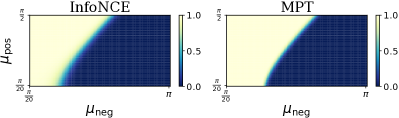
Figure 10: Average values of gradient dissipation term under different $\mu_{\mathrm{pos}}$-$\mu_{\mathrm{neg}}$ pairs for InfoNCE and MPT

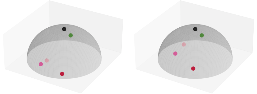
(a) The gap between the anchor-positive and anchor-negative distances is larger in the representation space trained without gradient dissipation (left) compared to that with gradient dissipation (right).

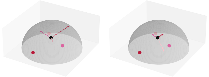
(b) When not amplified by the weight term, the contribution of the hardest negative samples to the optimization direction is minimal (left). Once amplified by the weight term, the hardest negative samples dominate the optimization direction (right).

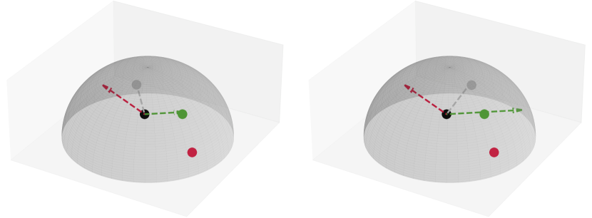
(c) When the ratio term does not meet the conditions in Lemma 1, anchor-positive distance increases after optimization. When the conditions are met, anchor-positive distance decreases after optimization.

Figure 11: Illustrations for the role in optimization of each component.

We first present the results of experimenting the gradient dissipation term for InfoNCE and MET (refer to Section 3.1) in Figure 11(a).

Then, we provide three illustrations in Figure 11 to facilitate an intuitive understanding of the roles played by different components in optimizing the representation space. In the diagram, black dots represent the anchor, gray dots represent the positions of the anchor after optimization, green dots represent positive samples, and red dots represent negative samples. Among the negative samples, the lighter the shade of red, the harder the negative sample is.

Appendix C Proof of Lemma 1

For the anchor point $h_{i}$, let us denote the angle between it and the positive sample $h_{i}^{\prime}$ as $\theta_{ii^{\prime}}$, and the angle between it and the negative sample $h_{j}^{\prime}$ as $\theta_{ij^{\prime}}$. Let $\alpha$ represent the dihedral angle between the planes $Oh_{i}h_{i}^{\prime}$ and $Oh_{i}h_{j}^{\prime}$. Under the influence of the optimization direction $\lambda(rh_{i}^{\prime}-h_{j}^{\prime})$, the new position of the anchor point after movement is denoted as $h_{i}^{n}$. Although all embeddings lie on a hypersphere, to simplify the proof process, we orthogonally project all embeddings onto the tangent plane at the anchor $h_{i}$ (as shown in Figure 12). In this case, the length of line $h_{i}h_{i}^{\prime}$ is equal to $\sin(\theta_{ii^{\prime}})$, the length of line $h_{i}h_{j}^{\prime}$ is equal to $\sin(\theta_{ij^{\prime}})$, and the angle $\angle h_{i}^{\prime}h_{i}h_{j}^{\prime}$ is $\alpha$. This simplification is reasonable because the optimization of the anchor $h_{i}$ on the hypersphere can in fact be considered as optimization on the tangent plane, which is then projected back onto the hypersphere. For the optimization direction $\lambda(rh_{i}^{\prime}-h_{j}^{\prime})$, we also project it onto the tangent plane, where $-\lambda h_{j}^{\prime}$ corresponds to the line $h_{i}c$, and $\lambda rh_{i}^{\prime}$ corresponds to line $ch_{i}^{n}$.

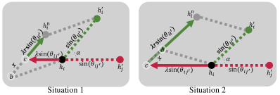
Figure 12: Illustrations of the proof to Lemma 1

Then, to ensure that the anchor-positive distance does not increase after optimization (i.e., $h_{i}^{n}h_{i}^{\prime}\leq h_{i}h_{i}^{\prime}$), we assume $h_{i}^{n}h_{i}^{\prime}=h_{i}h_{i}^{\prime}=\sin(\theta_{ii^{\prime}})$, thereby obtaining the necessary boundary condition that satisfies the requirement. Specifically, by deriving the relationship between $r$ and the other elements at this time, we can obtain the lower bound of $r$ that satisfies the requirements. To this end, we add an auxiliary point $b$ on the line $ch_{i}^{n}$, such that the quadrilateral $bh_{i}^{n}h_{i}^{\prime}h_{i}$ forms a rhombus (two possible situations when adding the auxiliary point are given in Figure 12), and we denote the length of the line $bc$ as $x$. By applying the cosine theorem, we can obtain the following: under Situation 1, we have

$$x_{1}= -\lambda\sin(\theta_{ij^{\prime}})\cos(\alpha)$$

$$+\sqrt{\sin^{2}(\theta_{ii^{\prime}})-\lambda^{2}\sin^{2}(\theta_{ij^{\prime}})\sin^{2}(\alpha)};$$

under Situation 2, we have

$$x_{2}= \lambda\sin(\theta_{ij^{\prime}})\cos(\alpha)$$

$$-\sqrt{\sin^{2}(\theta_{ii^{\prime}})-\lambda^{2}\sin^{2}(\theta_{ij^{\prime}})\sin^{2}(\alpha)}.$$

At this point, we can express $r$ as follows:

$$r =\frac{\sin(\theta_{ii^{\prime}})-x_{1}}{\lambda\sin(\theta_{ii^{\prime}})}=\frac{\sin(\theta_{ii^{\prime}})+x_{2}}{\lambda\sin(\theta_{ii^{\prime}})}$$

$$=\frac{1}{\lambda}+\frac{\sin\theta_{ij^{\prime}}\cos\alpha}{\sin\theta_{ii^{\prime}}}-\sqrt{\frac{1}{\lambda^{2}}-\frac{\sin^{2}\theta_{ij^{\prime}}\sin^{2}\alpha}{\sin^{2}\theta_{ii^{\prime}}}},$$

which is the lower bound of $r$ that satisfies the requirements, thus proving Lemma 1.

Appendix D Gradients of Optimization Objectives

D.1 Gradients of effective Objectives

In this section, we provide the derivation process of gradients in Section 2. The gradient of $\mathcal{L}^{\mathrm{info}}_{i}$ w.r.t $h_{i}$ is

$$\frac{\partial\mathcal{L}^{\mathrm{info}}_{i}}{\partial h_{i}}= \frac{\partial}{\partial h_{i}}\left(-\log\frac{e^{h_{i}^{\top}h_{i}^{\prime}/\tau}}{\sum_{j=1}^{N}e^{h_{i}^{\top}h_{j}^{\prime}/\tau}}\right)$$

$$= \frac{\partial(\log\sum_{j=1}^{N}e^{h_{i}^{\top}h_{j}^{\prime}/\tau})}{\partial h_{i}}-\frac{\partial h_{i}^{\top}h_{i}^{\prime}/\tau}{\partial h_{i}}$$

$$= \frac{\partial\sum_{j=1}^{N}e^{h_{i}^{\top}h_{j}^{\prime}/\tau}/\partial h_{i}}{\sum_{j=1}^{N}e^{h_{i}^{\top}h_{j}^{\prime}/\tau}}-\frac{h_{i}^{\prime}}{\tau}$$

$$= \frac{\sum_{j=1}^{N}e^{h_{i}^{\top}h_{j}^{\prime}/\tau}h_{j}^{\prime}}{\tau\sum_{j=1}^{N}e^{h_{i}^{\top}h_{j}^{\prime}/\tau}}-\frac{h_{i}^{\prime}}{\tau}$$

$$= \frac{\sum_{j\neq i}^{N}e^{h_{i}^{\top}h_{j}^{\prime}/\tau}(h_{j}^{\prime}-h_{i}^{\prime})}{\tau\sum_{j=1}^{N}e^{h_{i}^{\top}h_{j}^{\prime}/\tau}}.$$

The gradient of $\mathcal{L}^{\mathrm{arc}}_{i}$ w.r.t $h_{i}$ is

$$\frac{\partial\mathcal{L}^{\mathrm{arc}}_{i}}{\partial h_{i}}= \frac{\partial}{\partial h_{i}}\left(-\log\frac{e^{\frac{\cos(\theta_{ii^{\prime}}+u)}{\tau}}}{e^{\frac{\cos(\theta_{ii^{\prime}}+u)}{\tau}}+\sum\limits_{j\neq i}^{N}e^{\frac{h_{i}^{\top}h_{j}^{\prime}}{\tau}}}\right)$$

$$= \frac{\partial\log(e^{\cos(\theta_{ii^{\prime}}+u)/\tau}+\sum_{j\neq i}^{N}e^{h_{i}^{\top}h_{j}^{\prime}/\tau})}{\partial h_{i}}$$

$$-\frac{\partial\cos(\theta_{ii^{\prime}}+u)/\tau}{\partial h_{i}}$$

$$= \frac{\partial(e^{\cos(\theta_{ii^{\prime}}+u)/\tau}+\sum_{j\neq i}^{N}e^{h_{i}^{\top}h_{j}^{\prime}/\tau})/\partial h_{i}}{e^{\cos(\theta_{ii^{\prime}}+u)/\tau}+\sum_{j\neq i}^{N}e^{h_{i}^{\top}h_{j}^{\prime}/\tau}}$$

$$+\frac{\sin(\theta_{ii^{\prime}}+u)}{\tau}\cdot\frac{\partial(\theta_{ii^{\prime}}+u)}{\partial h_{i}}$$

$$= \frac{e^{\cos(\theta_{ii^{\prime}}+u)/\tau}\cdot\frac{\sin(\theta_{ii^{\prime}}+u)}{\sin(\theta_{ii^{\prime}})}h_{i}^{\prime}}{\tau(e^{\cos(\theta_{ii^{\prime}}+u)/\tau}+\sum_{j\neq i}^{N}e^{h_{i}^{\top}h_{j}^{\prime}/\tau})}$$

$$+\frac{\sum_{j\neq i}^{N}e^{h_{i}^{\top}h_{j}^{\prime}/\tau}h_{j}^{\prime}}{\tau(e^{\cos(\theta_{ii^{\prime}}+u)/\tau}+\sum_{j\neq i}^{N}e^{h_{i}^{\top}h_{j}^{\prime}/\tau})}$$

$$-\frac{\sin(\theta_{ii^{\prime}}+u)}{\tau\sin(\theta_{ii^{\prime}})}h_{i}^{\prime}$$

$$= \frac{\sum_{j\neq i}^{N}e^{h_{i}^{\top}h_{j}^{\prime}/\tau}(h_{j}^{\prime}-\frac{\sin(\theta_{ii^{\prime}}+u)}{\sin(\theta_{ii^{\prime}})}h_{i}^{\prime})}{\tau(e^{\cos(\theta_{ii^{\prime}}+u)/\tau}+\sum_{j\neq i}^{N}e^{h_{i}^{\top}h_{j}^{\prime}/\tau})}.$$

The gradient of $\mathcal{L}^{\mathrm{tri}}_{i}$ w.r.t $h_{i}$ is

$$\frac{\partial\mathcal{L}^{\mathrm{tri}}_{i}}{\partial h_{i}}= \mathbb{I}_{\{-d(h_{i},h_{i}^{\prime})+d(h_{i},h_{j}^{\prime})<m\}}$$

$$\times\left(\frac{\partial d(h_{i},h_{i}^{\prime})}{\partial h_{i}}-\frac{\partial d(h_{i},h_{j}^{\prime})}{\partial h_{i}}\right),$$

where $j=\arg\min_{k\neq i}d(h_{i},h_{k}^{\prime})$. Therefore, The gradient of $\mathcal{L}^{\mathrm{mpt}}_{i}$ w.r.t $h_{i}$ is

$$\frac{\partial\mathcal{L}^{\mathrm{mpt}}_{i}}{\partial h_{i}}=\mathbb{I}_{\{h_{i}^{\top}h_{i}^{\prime}-h_{i}^{\top}h_{j}^{\prime}<m\}}(h_{j}^{\prime}-h_{i}^{\prime}),$$

and the gradient of $\mathcal{L}^{\mathrm{met}}_{i}$ w.r.t $h_{i}$ is

$$\frac{\partial\mathcal{L}^{\mathrm{met}}_{i}}{\partial h_{i}}= \mathbb{I}_{\{\|h_{i}-h_{i}^{\prime}\|_{2}-\|h_{i}-h_{j}^{\prime}\|<m\}}$$

$$\times\left(\frac{h_{j}^{\prime}}{\|h_{i}-h_{j}^{\prime}\|_{2}}-\frac{h_{i}^{\prime}}{\|h_{i}-h_{i}^{\prime}\|}\right).$$

D.2 Gradients of Ineffective Objectives

In this section, we provide the gradients of objectives in Section 4.The gradient of $\mathcal{L}^{\mathrm{a}}$ w.r.t $h_{i}$ is

$$\frac{\partial\mathcal{L}^{\mathrm{a}}}{\partial h_{i}}=-\frac{2}{N}h_{i}^{\prime},$$ (7)

the gradient of $\mathcal{L}^{\mathrm{u,MHE}}$ w.r.t $h_{i}$ is

$$\frac{\partial\mathcal{L}^{\mathrm{u,MHE}}}{\partial h_{i}}=\frac{\sum_{j\neq i}^{N}2e^{2h_{i}^{\top}h_{j}}h_{j}}{\sum_{1\leq k<l\leq N}e^{2h_{k}^{\top}h_{l}}},$$ (8)

and the gradient of $\mathcal{L}^{\mathrm{u,MHS}}$ w.r.t $h_{i}$ is

$$\frac{\partial\mathcal{L}^{\mathrm{u,MHS}}}{\partial h_{i}}=\frac{1}{\|h_{i}-h_{j}\|_{2}}h_{j},$$ (9)

where $j=\arg\min_{j\neq i}\|h_{i}-h_{j}\|$.

The gradients of $\mathcal{L}^{\mathrm{B}}$ and $\mathcal{L}^{\mathrm{V}}$ w.r.t $h_{i}$ have been derived by Tao et al. (2022):

$$\frac{\partial\mathcal{L}^{\mathrm{B}}}{\partial h_{i}}=\frac{2}{N}(-Ah_{i}^{\prime}+\nu^{\mathrm{B}}\sum_{j\neq i}^{N}\frac{h_{i}^{\prime\top}h_{j}^{\prime}}{N}h_{j}),$$ (10)

where $A=I-(1-\nu^{\mathrm{B}})C^{\mathrm{B}}_{\mathrm{diag}}$, and $C^{\mathrm{B}}_{\mathrm{diag}}$ is the diagonal matrix of $C^{\mathrm{B}}$, and

$$\frac{\partial\mathcal{L}^{\mathrm{V}}}{\partial h_{i}}=\frac{2}{N}(-h_{i}^{\prime}+\nu^{\mathrm{V}}\sum_{j\neq i}^{N}\frac{h_{i}^{\top}h_{j}}{N}h_{j}),$$ (11)

where $\nu^{\mathrm{V}}=\frac{2\nu^{\mathrm{V,1}}N^{2}}{D(N-1)^{2}}$. Note that the original Barlow Twins adopts a batch normalization, and VICReg adopts a de-center operation, which is different from the commonly used $l_{2}$ normalization in SRL. But Tao et al. (2022) verify that these operations have a similar effect in training, therefore we use $l_{2}$ normalization for all losses for consistency.

One more thing to note is that the gradients of ineffective losses are mapped into the following form:

$$\frac{\partial\mathcal{L}_{i}}{\partial h_{i}}=\mathrm{GD}(\cdot)\sum_{j\neq i}^{N}\mathrm{W}(\cdot)(h_{j}-\mathrm{R}(\cdot)h_{i}^{\prime}),$$ (12)

which uses $h_{j}$ instead of $h_{j}^{\prime}$ in Equation 4. Since $h_{j}$ and $h_{j}^{\prime}$ are mathematically equivalent with respect to $h_{i}$, we consider Equation 4 and 12 to be consistent and only present Equation 4 in the main body of the paper.

Appendix E Modifications to Ineffective Losses

We offer two methods of modification: (1) modifying the gradient-equivalent form of the optimization objective, which is the method to modify Barlow Twins in Section 4, and (2) directly modifying the optimization objective itself.

For VICReg, we use the first method for modification as we do for Barlow Twins. Based on gradients, the optimization objective of VICReg is equivalent to

$$\mathcal{L}^{\mathrm{eV}}_{i}=-h_{i}^{\top}w_{\mathrm{p},i}^{\mathrm{V}}h_{i}^{\prime}+\nu^{\mathrm{V}}\sum_{j\neq i}^{N}h_{i}^{\top}w_{\mathrm{n},ij}^{\mathrm{V}}h_{j},$$

where $w_{\mathrm{p},i}^{\mathrm{V}}=\frac{2I}{N},w_{\mathrm{n},ij}^{\mathrm{V}}=\frac{2h_{i}^{\top}h_{j}I}{N^{2}}$, and both of them do not require gradient. To adjust the gradient dissipation term, we stop the gradient of anchor $h_{i}$ that does not meet the condition ($h_{i}^{\top}h_{i}^{\prime}-\max_{k\neq i}^{N}h_{i}^{\top}h_{k}^{\prime}<m$), which is equivalent to multiplying the loss by the indicator function

$$d_{i}=\mathbb{I}_{\{h_{i}^{\top}h_{i}^{\prime}-\max_{k\neq i}^{N}h_{i}^{\top}h_{k}^{\prime}<m\}}.$$

To adjust the weight term, we first set $\nu^{\mathrm{V}}=1$. Then, we modify $w_{\mathrm{n},ij}^{\mathrm{V}}$ to an exponential form:

$$w_{\mathrm{n},ij}^{\mathrm{mV}}=\frac{e^{h_{i}^{\top}h_{j}/\tau}}{\sum_{k\neq l}e^{h_{k}^{\top}h_{l}/\tau}}.$$

To adjust the ratio term, we set the loss to have a static ratio $r$, by modifying $w_{\mathrm{p},i}^{\mathrm{V}}$ to

$$w_{\mathrm{p},i}^{\mathrm{mV}}=\sum_{j\neq i}^{N}w_{\mathrm{n},ij}^{\mathrm{mV}}=\frac{r\sum_{j\neq i}^{N}e^{h_{i}^{\top}h_{j}/\tau}}{\sum_{k\neq l}e^{h_{k}^{\top}h_{l}/\tau}},$$

which do not require gradients. Finally, the modified VICReg can be represented as

$$\mathcal{L}_{i}^{\mathrm{mV}}=d_{i}(-h_{i}^{\top}w_{\mathrm{p},i}^{\mathrm{mV}}h_{i}^{\prime}+\sum_{j\neq i}^{N}h_{i}^{\top}w_{\mathrm{n},ij}^{\mathrm{mV}}h_{j}).$$ (13)

For alignment and uniformity, we use the second method for modification. To adjust the gradient dissipation term, we stop the gradient of anchor $h_{i}$ that does not meet the condition ($h_{i}^{\top}h_{i}^{\prime}-\max_{k\neq i}^{N}h_{i}^{\top}h_{k}^{\prime}<m$) as before. As for the weight term, since the weight term of ($\mathcal{L}^{\mathrm{a}}+\nu^{\mathrm{u}}\mathcal{L}^{\mathrm{u,MHS}}$) does not require adjustment, we only adjust the weight term for ($\mathcal{L}^{\mathrm{a}}+\nu^{\mathrm{u}}\mathcal{L}^{\mathrm{u,MHE}}$). Specifically, We set $\nu^{\mathrm{u}}=1$ and introduce a temperature parameter $\tau$ to $\mathcal{L}^{\mathrm{u,MHE}}$:

$$\mathcal{L}^{\mathrm{u,mMHE}}=\log\frac{2\sum_{1\leq k<l\leq N}e^{-\|h_{k}-h_{l}\|_{2}^{2}/(2\tau)}}{N(N-1)}.$$

To adjust the ratio term, we modify both of them to have a static ratio $r$ by prepending a coefficient to the alignment:

$$\mathcal{L}_{i}^{\mathrm{a,mMHE}} =\underbrace{\frac{r\sum_{j\neq i}^{N}e^{h_{i}^{\top}h_{j}/\tau}}{2\tau\sum_{1\leq k<l\leq N}e^{h_{k}^{\top}h_{l}/\tau}}}_{\mathrm{no\ gradient}}\|h_{i}-h_{i}^{\prime}\|_{2}^{2},$$

$$\mathcal{L}_{i}^{\mathrm{a,mMHS}} =\underbrace{\frac{r}{2\max_{j\neq i}\|h_{i}-h_{j}\|_{2}}}_{\mathrm{no\ gradient}}\|h_{i}-h_{i}^{\prime}\|_{2}^{2}.$$

Finally, the modified losses can be represented as

$$\mathcal{L}_{i}^{\mathrm{mMHE}} =d_{i}(\mathcal{L}_{i}^{\mathrm{a,mMHE}}+\mathcal{L}^{\mathrm{u,mMHE}}),$$ (14)

$$\mathcal{L}_{i}^{\mathrm{mMHS}} =d_{i}(\mathcal{L}_{i}^{\mathrm{a,mMHS}}+\mathcal{L}_{i}^{\mathrm{u,MHS}}).$$ (15)

In order to verify the correctness of the modification, we present the gradients of all the modified losses here. The gradient of $\mathcal{L}_{i}^{\mathrm{mMHE}}$ w.r.t $h_{i}$ is

$$\frac{\mathcal{L}_{i}^{\mathrm{mMHE}}}{\partial h_{i}}=d_{i}\frac{\sum_{j\neq i}^{N}e^{h_{i}^{\top}h_{j}/\tau}(h_{j}-rh_{i}^{\prime})}{\tau\sum_{1\leq k<l\leq N}e^{h_{k}^{\top}h_{l}/\tau}}.$$ (16)

The gradient of $\mathcal{L}_{i}^{\mathrm{mMHS}}$ w.r.t $h_{i}$ is

$$\frac{\mathcal{L}_{i}^{\mathrm{mMHE}}}{\partial h_{i}}=d_{i}\frac{(h_{j}-rh_{i}^{\prime})}{\|h_{i}-h_{j}\|_{2}},$$ (17)

where $j=\arg\min_{k\neq i}\|h_{i}-h_{k}\|_{2}$. The gradient of $\mathcal{L}_{i}^{\mathrm{mB}}$ w.r.t $h_{i}$ is

$$\frac{\mathcal{L}_{i}^{\mathrm{mB}}}{\partial h_{i}}=d_{i}\frac{\sum_{j\neq i}^{N}e^{h_{i}^{\prime\top}h_{j}^{\prime}/\tau}(h_{j}-rh_{i}^{\prime})}{\sum_{k\neq l}^{N}e^{h_{k}^{\prime\top}h_{l}^{\prime}/\tau}}.$$ (18)

The gradient of $\mathcal{L}_{i}^{\mathrm{mV}}$ w.r.t $h_{i}$ is

$$\frac{\mathcal{L}_{i}^{\mathrm{mV}}}{\partial h_{i}}=d_{i}\frac{\sum_{j\neq i}^{N}e^{h_{i}^{\top}h_{j}/\tau}(h_{j}-rh_{i}^{\prime})}{\sum_{k\neq l}^{N}e^{h_{k}^{\top}h_{l}/\tau}}.$$ (19)

References

- Agirre et al. (2015) Eneko Agirre, Carmen Banea, Claire Cardie, Daniel M. Cer, Mona T. Diab, Aitor Gonzalez-Agirre, Weiwei Guo, Iñigo Lopez-Gazpio, Montse Maritxalar, Rada Mihalcea, German Rigau, Larraitz Uria, and Janyce Wiebe. 2015. SemEval-2015 Task 2: Semantic Textual Similarity, English, Spanish and Pilot on Interpretability. In Proceedings of the 9th International Workshop on Semantic Evaluation, SemEval@NAACL-HLT 2015, Denver, Colorado, USA, June 4-5, 2015, pages 252–263. The Association for Computer Linguistics.
- Agirre et al. (2014) Eneko Agirre, Carmen Banea, Claire Cardie, Daniel M. Cer, Mona T. Diab, Aitor Gonzalez-Agirre, Weiwei Guo, Rada Mihalcea, German Rigau, and Janyce Wiebe. 2014. SemEval-2014 Task 10: Multilingual Semantic Textual Similarity. In Proceedings of the 8th International Workshop on Semantic Evaluation, SemEval@COLING 2014, Dublin, Ireland, August 23-24, 2014, pages 81–91. The Association for Computer Linguistics.
- Agirre et al. (2016) Eneko Agirre, Carmen Banea, Daniel M. Cer, Mona T. Diab, Aitor Gonzalez-Agirre, Rada Mihalcea, German Rigau, and Janyce Wiebe. 2016. SemEval-2016 Task 1: Semantic Textual Similarity, Monolingual and Cross-Lingual Evaluation. In Proceedings of the 10th International Workshop on Semantic Evaluation, SemEval@NAACL-HLT 2016, San Diego, CA, USA, June 16-17, 2016, pages 497–511. The Association for Computer Linguistics.
- Agirre et al. (2012) Eneko Agirre, Daniel M. Cer, Mona T. Diab, and Aitor Gonzalez-Agirre. 2012. SemEval-2012 Task 6: A Pilot on Semantic Textual Similarity. In Proceedings of the 6th International Workshop on Semantic Evaluation, SemEval@NAACL-HLT 2012, Montréal, Canada, June 7-8, 2012, pages 385–393. The Association for Computer Linguistics.
- Agirre et al. (2013) Eneko Agirre, Daniel M. Cer, Mona T. Diab, Aitor Gonzalez-Agirre, and Weiwei Guo. 2013. *SEM 2013 shared task: Semantic Textual Similarity. In Proceedings of the Second Joint Conference on Lexical and Computational Semantics, *SEM 2013, June 13-14, 2013, Atlanta, Georgia, USA, pages 32–43. Association for Computational Linguistics.
- Balestriero and LeCun (2022) Randall Balestriero and Yann LeCun. 2022. Contrastive and Non-Contrastive Self-Supervised Learning Recover Global and Local Spectral Embedding Methods. In Advances in Neural Information Processing Systems 35: Annual Conference on Neural Information Processing Systems 2022, NeurIPS 2022, New Orleans, LA, USA, November 28 - December 9, 2022.
- Bardes et al. (2022) Adrien Bardes, Jean Ponce, and Yann LeCun. 2022. VICReg: Variance-Invariance-Covariance Regularization for Self-Supervised Learning. In The Tenth International Conference on Learning Representations, ICLR 2022, Virtual Event, April 25-29, 2022. OpenReview.net.
- Cer et al. (2017) Daniel M. Cer, Mona T. Diab, Eneko Agirre, Iñigo Lopez-Gazpio, and Lucia Specia. 2017. SemEval-2017 Task 1: Semantic Textual Similarity Multilingual and Crosslingual Focused Evaluation. In Proceedings of the 11th International Workshop on Semantic Evaluation, SemEval@ACL 2017, Vancouver, Canada, August 3-4, 2017, pages 1–14. Association for Computational Linguistics.
- Conneau and Kiela (2018) Alexis Conneau and Douwe Kiela. 2018. SentEval: An Evaluation Toolkit for Universal Sentence Representations. In Proceedings of the Eleventh International Conference on Language Resources and Evaluation, LREC 2018, Miyazaki, Japan, May 7-12, 2018. European Language Resources Association (ELRA).
- Devlin et al. (2019) Jacob Devlin, Ming-Wei Chang, Kenton Lee, and Kristina Toutanova. 2019. BERT: Pre-training of Deep Bidirectional Transformers for Language Understanding. In Proceedings of the 2019 Conference of the North American Chapter of the Association for Computational Linguistics: Human Language Technologies, NAACL-HLT 2019, Minneapolis, MN, USA, June 2-7, 2019, Volume 1 (Long and Short Papers), pages 4171–4186. Association for Computational Linguistics.
- Dolan and Brockett (2005) William B. Dolan and Chris Brockett. 2005. Automatically Constructing a Corpus of Sentential Paraphrases. In Proceedings of the Third International Workshop on Paraphrasing, IWP@IJCNLP 2005, Jeju Island, Korea, October 2005, 2005. Asian Federation of Natural Language Processing.
- Gao et al. (2021) Tianyu Gao, Xingcheng Yao, and Danqi Chen. 2021. SimCSE: Simple Contrastive Learning of Sentence Embeddings. In Proceedings of the 2021 Conference on Empirical Methods in Natural Language Processing, EMNLP 2021, Virtual Event / Punta Cana, Dominican Republic, 7-11 November, 2021, pages 6894–6910. Association for Computational Linguistics.
- Gao et al. (2023) Yunfan Gao, Yun Xiong, Xinyu Gao, Kangxiang Jia, Jinliu Pan, Yuxi Bi, Yi Dai, Jiawei Sun, Qianyu Guo, Meng Wang, and Haofen Wang. 2023. Retrieval-Augmented Generation for Large Language Models: A Survey. CoRR, abs/2312.10997. ArXiv: 2312.10997.
- Garrido et al. (2023) Quentin Garrido, Yubei Chen, Adrien Bardes, Laurent Najman, and Yann LeCun. 2023. On the duality between contrastive and non-contrastive self-supervised learning. In The Eleventh International Conference on Learning Representations, ICLR 2023, Kigali, Rwanda, May 1-5, 2023. OpenReview.net.
- Hu and Liu (2004) Minqing Hu and Bing Liu. 2004. Mining and summarizing customer reviews. In Proceedings of the Tenth ACM SIGKDD International Conference on Knowledge Discovery and Data Mining, Seattle, Washington, USA, August 22-25, 2004, pages 168–177. ACM.
- Jiang et al. (2022) Ting Jiang, Jian Jiao, Shaohan Huang, Zihan Zhang, Deqing Wang, Fuzhen Zhuang, Furu Wei, Haizhen Huang, Denvy Deng, and Qi Zhang. 2022. PromptBERT: Improving BERT Sentence Embeddings with Prompts. In Proceedings of the 2022 Conference on Empirical Methods in Natural Language Processing, EMNLP 2022, Abu Dhabi, United Arab Emirates, December 7-11, 2022, pages 8826–8837. Association for Computational Linguistics.
- Klein and Nabi (2022) Tassilo Klein and Moin Nabi. 2022. SCD: Self-Contrastive Decorrelation of Sentence Embeddings. In Proceedings of the 60th Annual Meeting of the Association for Computational Linguistics (Volume 2: Short Papers), ACL 2022, Dublin, Ireland, May 22-27, 2022, pages 394–400. Association for Computational Linguistics.
- Li et al. (2020) Bohan Li, Hao Zhou, Junxian He, Mingxuan Wang, Yiming Yang, and Lei Li. 2020. On the Sentence Embeddings from Pre-trained Language Models. In Proceedings of the 2020 Conference on Empirical Methods in Natural Language Processing, EMNLP 2020, Online, November 16-20, 2020, pages 9119–9130. Association for Computational Linguistics.
- Liu et al. (2021) Weiyang Liu, Rongmei Lin, Zhen Liu, Li Xiong, Bernhard Schölkopf, and Adrian Weller. 2021. Learning with Hyperspherical Uniformity. In The 24th International Conference on Artificial Intelligence and Statistics, AISTATS 2021, April 13-15, 2021, Virtual Event, volume 130 of Proceedings of Machine Learning Research, pages 1180–1188. PMLR.
- Liu et al. (2019) Yinhan Liu, Myle Ott, Naman Goyal, Jingfei Du, Mandar Joshi, Danqi Chen, Omer Levy, Mike Lewis, Luke Zettlemoyer, and Veselin Stoyanov. 2019. RoBERTa: A Robustly Optimized BERT Pretraining Approach. CoRR, abs/1907.11692. ArXiv: 1907.11692.
- Marelli et al. (2014) Marco Marelli, Stefano Menini, Marco Baroni, Luisa Bentivogli, Raffaella Bernardi, and Roberto Zamparelli. 2014. A SICK cure for the evaluation of compositional distributional semantic models. In Proceedings of the Ninth International Conference on Language Resources and Evaluation, LREC 2014, Reykjavik, Iceland, May 26-31, 2014, pages 216–223. European Language Resources Association (ELRA).
- Nie et al. (2023) Zhijie Nie, Richong Zhang, and Yongyi Mao. 2023. On The Inadequacy of Optimizing Alignment and Uniformity in Contrastive Learning of Sentence Representations. In The Eleventh International Conference on Learning Representations, ICLR 2023, Kigali, Rwanda, May 1-5, 2023. OpenReview.net.
- Oord et al. (2018) Aäron van den Oord, Yazhe Li, and Oriol Vinyals. 2018. Representation Learning with Contrastive Predictive Coding. CoRR, abs/1807.03748. ArXiv: 1807.03748.
- Pang and Lee (2004) Bo Pang and Lillian Lee. 2004. A Sentimental Education: Sentiment Analysis Using Subjectivity Summarization Based on Minimum Cuts. In Proceedings of the 42nd Annual Meeting of the Association for Computational Linguistics, 21-26 July, 2004, Barcelona, Spain, pages 271–278. ACL.
- Pang and Lee (2005) Bo Pang and Lillian Lee. 2005. Seeing Stars: Exploiting Class Relationships for Sentiment Categorization with Respect to Rating Scales. In ACL 2005, 43rd Annual Meeting of the Association for Computational Linguistics, Proceedings of the Conference, 25-30 June 2005, University of Michigan, USA, pages 115–124. The Association for Computer Linguistics.
- Shi et al. (2023) Zhan Shi, Guoyin Wang, Ke Bai, Jiwei Li, Xiang Li, Qingjun Cui, Belinda Zeng, Trishul Chilimbi, and Xiaodan Zhu. 2023. OssCSE: Overcoming Surface Structure Bias in Contrastive Learning for Unsupervised Sentence Embedding. In Proceedings of the 2023 Conference on Empirical Methods in Natural Language Processing, EMNLP 2023, Singapore, December 6-10, 2023, pages 7242–7254. Association for Computational Linguistics.
- Socher et al. (2013) Richard Socher, Alex Perelygin, Jean Wu, Jason Chuang, Christopher D. Manning, Andrew Y. Ng, and Christopher Potts. 2013. Recursive Deep Models for Semantic Compositionality Over a Sentiment Treebank. In Proceedings of the 2013 Conference on Empirical Methods in Natural Language Processing, EMNLP 2013, 18-21 October 2013, Grand Hyatt Seattle, Seattle, Washington, USA, A meeting of SIGDAT, a Special Interest Group of the ACL, pages 1631–1642. ACL.
- Tao et al. (2022) Chenxin Tao, Honghui Wang, Xizhou Zhu, Jiahua Dong, Shiji Song, Gao Huang, and Jifeng Dai. 2022. Exploring the Equivalence of Siamese Self-Supervised Learning via A Unified Gradient Framework. In IEEE/CVF Conference on Computer Vision and Pattern Recognition, CVPR 2022, New Orleans, LA, USA, June 18-24, 2022, pages 14411–14420. IEEE.
- Voorhees and Tice (2000) Ellen M. Voorhees and Dawn M. Tice. 2000. Building a question answering test collection. In SIGIR 2000: Proceedings of the 23rd Annual International ACM SIGIR Conference on Research and Development in Information Retrieval, July 24-28, 2000, Athens, Greece, pages 200–207. ACM.
- Wang and Isola (2020) Tongzhou Wang and Phillip Isola. 2020. Understanding Contrastive Representation Learning through Alignment and Uniformity on the Hypersphere. In Proceedings of the 37th International Conference on Machine Learning, ICML 2020, 13-18 July 2020, Virtual Event, volume 119 of Proceedings of Machine Learning Research, pages 9929–9939. PMLR.
- Wiebe et al. (2005) Janyce Wiebe, Theresa Wilson, and Claire Cardie. 2005. Annotating Expressions of Opinions and Emotions in Language. Lang. Resour. Evaluation, 39(2-3):165–210.
- Xu et al. (2023) Jiahao Xu, Wei Shao, Lihui Chen, and Lemao Liu. 2023. SimCSE++: Improving Contrastive Learning for Sentence Embeddings from Two Perspectives. In Proceedings of the 2023 Conference on Empirical Methods in Natural Language Processing, EMNLP 2023, Singapore, December 6-10, 2023, pages 12028–12040. Association for Computational Linguistics.
- Yan et al. (2021) Yuanmeng Yan, Rumei Li, Sirui Wang, Fuzheng Zhang, Wei Wu, and Weiran Xu. 2021. ConSERT: A Contrastive Framework for Self-Supervised Sentence Representation Transfer. In Proceedings of the 59th Annual Meeting of the Association for Computational Linguistics and the 11th International Joint Conference on Natural Language Processing, ACL/IJCNLP 2021, (Volume 1: Long Papers), Virtual Event, August 1-6, 2021, pages 5065–5075. Association for Computational Linguistics.
- Zbontar et al. (2021) Jure Zbontar, Li Jing, Ishan Misra, Yann LeCun, and Stéphane Deny. 2021. Barlow Twins: Self-Supervised Learning via Redundancy Reduction. In Proceedings of the 38th International Conference on Machine Learning, ICML 2021, 18-24 July 2021, Virtual Event, volume 139 of Proceedings of Machine Learning Research, pages 12310–12320. PMLR.
- Zhang et al. (2022a) Yanzhao Zhang, Richong Zhang, Samuel Mensah, Xudong Liu, and Yongyi Mao. 2022a. Unsupervised Sentence Representation via Contrastive Learning with Mixing Negatives. In Thirty-Sixth AAAI Conference on Artificial Intelligence, AAAI 2022, Thirty-Fourth Conference on Innovative Applications of Artificial Intelligence, IAAI 2022, The Twelveth Symposium on Educational Advances in Artificial Intelligence, EAAI 2022 Virtual Event, February 22 - March 1, 2022, pages 11730–11738. AAAI Press.
- Zhang et al. (2022b) Yuhao Zhang, Hongji Zhu, Yongliang Wang, Nan Xu, Xiaobo Li, and Binqiang Zhao. 2022b. A Contrastive Framework for Learning Sentence Representations from Pairwise and Triple-wise Perspective in Angular Space. In Proceedings of the 60th Annual Meeting of the Association for Computational Linguistics (Volume 1: Long Papers), ACL 2022, Dublin, Ireland, May 22-27, 2022, pages 4892–4903. Association for Computational Linguistics.