Enhanced detection of time-dependent dielectric structure:
Rayleigh’s limit and quantum vacuum

Abstract

Detection of scattered light can determine the susceptibility of dielectrics. It is normally limited by Rayleigh’s limit: details finer than the wavelength of the incident light cannot be determined from the far-field domain. We show that putting the dielectric in motion can be useful for determining its susceptibility. This inverse quantum optics problem is studied in two different versions: (i) A spatially and temporally modulated metamaterial, whose dielectric permeability is similar to that of moving dielectrics. (ii) A dielectric moving with a constant velocity, a problem we studied within relativistic optics. Certain features of the susceptibility can be determined without shining any incident field on the dielectric because the vacuum contribution to the photodetection signal is non-zero due to the negative frequencies. When the incident light is shined, the determination of dielectric susceptibility is enhanced and and goes beyond the classical Rayleigh limit; it pertains to evanescent waves for (ii), but reaches the far-field domain for (i).

Inverse optics measures the dielectric susceptibility of materials by shining (incident) light with known characteristics on them and detecting scattered light Baltes et al. (1980); Devaney (2012). Recent advances in inverse optics relate to using quantum features of the incident light Shih et. al. (2001); Abouraddy et al. (2002); Boto et. al. (2000); Santos et al. (2003); Liu et al. (2021); Avetisyan et al. (2023). In particular, quantum features improve on classical Rayleigh’s limit that bounds the far-field resolution of dielectric susceptibility, given the wavelength of the incident light. While the improvement is possible (e.g. up to eight times for two-photon light Avetisyan et al. (2023)), it also connects with difficulties of preparing specific quantum states of light and with having prior information on the dielectric sample Avetisyan et al. (2023).

We look for further resources, which will allow better resolution. Our results identify one such resource that relies on the dielectric’s motion, or on imitating this motion via space-time modulation. Our proposal is dual to Doppler metrology Fang et al. (2021): we set the moving object to motion to determine its internal structure, rather than finding the velocity of the object.

The problem of moving dielectric has a fundamental appeal because it gave rise to special relativity Einstein (1905); Minkowski (1908); Pal (2021). Progress in this field was steady and impressive: the Fresnel-Fizeau drag, the Doppler effect(s), the relativistic Snell–Descartes law, Cherenkov’s radiation Bolotovskii and Stolyarov (1975), light amplification via moving mirrors Kiefer (2014), etc. The quantization of the electromagnetic field in the presence of moving dielectric media Matloob (2005a, b); Horsley (2012) led to more recent results; e.g. the quantum friction phenomenon Horsley (2012); Mkrtchian (1995); Pendry (1997).

Electrodynamics of relativistically moving bodies has traditionally focused on electron clouds or plasma jets Bolotovskii and Stolyarov (1975); Mourou et al. (2006); Kiefer (2014). A recent activity in creating metamaterials with a space-time-modulated electric permeability renewed interest in this field Galiffi et al. (2022); Huidobro et al. (2019); Caloz et al. (2022). Though these metamaterials do not move, they are expected to mimic moving dielectrics.

Here we aim to show that motion or space-time modulation is a resource for improving resolution limits, i.e. seeing deeper into the dielectric structure. To this end, we develop scattering theory for two situations: (i) A spatially and temporally modulated metamaterial, whose dielectric susceptibility is similar to that of moving dielectrics. (ii) A dielectric moving with a constant velocity, a problem we studied within relativistic optics. These problems are related. For both (i) and (ii) we show that certain features of the dielectric can be determined from the quantum vacuum response, i.e. without shining any incident light on it. When shining is there, we show that (i) can overcome the classical Rayleigh resolution limit in the far-field situation. For (ii) a closely related effect is limited to the near-field.

Scattering theory. We develop quantum light scattering theory in space-time modulated isotropic dielectric metamaterials embedded in a vacuum. We work within quantum macroscopic electrodynamics, where the inhomogeneous, time-dependent dielectric is described via permeability $\varepsilon\left(\mathbf{r,}t\right)$ (no magnetic features), and the standard quantities for the electromagnetic field Landau et al. (2013):

$$\mathbf{D}\left(\mathbf{r,}t\right)=\varepsilon\left(\mathbf{r,}t\right)\mathbf{E}\left(\mathbf{r,}t\right),~{}~{}\mathbf{H}\left(\mathbf{r,}t\right)=\mathbf{B}\left(\mathbf{r,}t\right).$$ (1)

We use Gaussian units with $c=\hbar=\epsilon_{0}=1$. Employing (1) in Maxwell’s equation and excluding $\mathbf{B}$ leads to the Helmholtz equation for $\mathbf{E}$ Landau et al. (2013):

$$\partial_{\beta}\partial_{\beta}E_{\alpha}-\partial_{\alpha}\partial_{\beta}E_{\beta}-\partial_{t}^{2}E_{\alpha}=\partial_{t}^{2}[\bar{\varepsilon}E_{\alpha}],$$ (2)

$$\partial_{\alpha}\equiv\partial/\partial x_{\alpha},~{}~{}\bar{\varepsilon}\left(\mathbf{r,}t\right)\equiv\varepsilon\left(\mathbf{r,}t\right)-1,~{}~{}\alpha,\beta=1,2,3,$$ (3)

$$\mathbf{r}=(x_{1},x_{2},x_{3})=(x,y,z),$$ (4)

where repeated indices imply summation.

We assume that the electromagnetic field is quantized making (2) the Heisenberg equation for the operator $E_{\beta}$ Landau et al. (2013). But the matter is classical and has the average permeability $\varepsilon\left(\mathbf{r,}t\right)$ Landau et al. (2013). Hence, in (1) we left aside both the time-dispersion of dielectrics and its quantum features. Both are straightforward to include: time-dispersion will amount to an integral equation in (1), while the quantum features can be introduced via making $\varepsilon\left(\mathbf{r,}t\right)$ an operator and postponing the averaging over the dielectric state till the final results Landau et al. (2013). We avoid introducing these complications, as none of them are essential to our main results. For the same reason, we neglected anisotropy in $\varepsilon\left(\mathbf{r,}t\right)$.

Eqs. (1–4) apply to quantum optics, where intensities are standardly measured via photodetection Garrison and Chiao (2008). A photodetector is localized around position $\mathbf{r}$, works at an atomic transition frequency $\omega>0$ and measures e.g. the mean electric field intensity of the scattered radiation in the long-time limit Garrison and Chiao (2008)

$$I[\omega,\mathbf{r};|\psi\rangle\langle\psi|]=\langle\psi|{E}_{\alpha}^{\dagger}[\omega,\mathbf{r}]\,{E}_{\alpha}[\omega,\mathbf{r}]\,|\psi\rangle,~{}~{}\omega>0,$$ (5)

where $|\psi\rangle$ is the (initial) quantum state of the field, $\dagger$ means hermitian conjugation, and

$${E}_{\alpha}[\omega,\mathbf{r}]=\int\frac{{\rm d}t}{2\pi}e^{it\omega}{E}_{\alpha}(t,\mathbf{r})$$ (6)

is the Fourier transform of the electric field operator.

Within the standard setup of scattering $\mathbf{E}$ reads Devaney (2012):

$$\mathbf{E=E}^{[\text{in}]}+\mathbf{E}^{[\text{s}]},$$ (7)

where the incident field $\mathbf{E}^{[\text{in}]}(\mathbf{r},t)$ holds free Helmholtz’s equation, i.e. nullifies the left-hand-side of (2). Hence $\mathbf{E}^{[\text{in}]}$ has the standard quantized representation Garrison and Chiao (2008):

$$\mathbf{{E}}^{[\text{in}]}\left(\mathbf{r,}t\right)=\frac{i}{2\pi}\int{\rm d}\mathbf{q}\,\sqrt{q}\,\mathbf{e}_{\lambda}\left(\mathbf{q}\right)e^{i\left(\mathbf{q\cdot r}-qt\right)}{a}_{\lambda}\left(\mathbf{q}\right)+\text{h.c.},$$

$$\mathbf{q\cdot e_{\lambda}(q)}=0,\quad\mathbf{e_{\lambda}(q)\cdot e_{\lambda^{\prime}}(q)}=\delta_{\lambda\lambda^{\prime}},\quad\lambda=1,2,$$ (8)

$${\rm e}_{\lambda\alpha}\left(\mathbf{q}\right){\rm e}_{\lambda\beta}\left(\mathbf{q}\right)=\delta_{\alpha\beta}-{q}_{\alpha}{q}_{\beta}/q^{2},\quad q=|\mathbf{q}|,$$ (9)

$${a}_{\lambda}\left(\mathbf{q}\right){a}_{\lambda^{\prime}}^{\dagger}\left(\mathbf{q}^{\prime}\right)-{a}_{\lambda^{\prime}}^{\dagger}\left(\mathbf{q}^{\prime}\right){a}_{\lambda}\left(\mathbf{q}\right)=\delta_{\lambda\lambda^{\prime}}\delta\left(\mathbf{q-q}^{\prime}\right),$$ (10)

where $\mathbf{e}_{\lambda}\left(\mathbf{q}\right)$ is the real polarisation vector, $A+{\rm h.c.}=A+A^{\dagger}$, $\delta_{\lambda\lambda^{\prime}}$ is Kroenecker’s delta, and ${a}_{\lambda}(\mathbf{q})$ is the annihilation operator. Note that ${a}_{\lambda}(\mathbf{q})$ and ${a}_{\lambda^{\prime}}(\mathbf{q}^{\prime})$ commute. Eqs. (A113, 9) define orthogonality features of polarization vectors, where repeated $\lambda$ implies summation. Now $\mathbf{{E}}^{[\text{in}]}(\mathbf{r},t)$ contains contributions both from creation ${a}^{\dagger}_{\lambda}\left(\mathbf{q}\right)$ and annihilation ${a}_{\lambda}\left(\mathbf{q}\right)$ operators at (resp.) positive and negative frequencies, while only ${a}_{\lambda}\left(\mathbf{q}\right)$ contribute to $\mathbf{{E}}^{[\text{in}]}[\omega>0,\mathbf{r}]$.

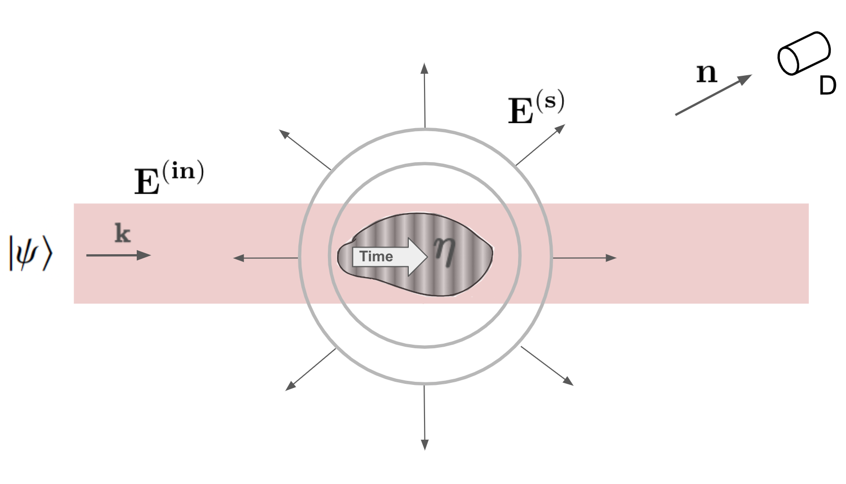
Figure 1: Scattering from resting, space-time-modulated dielectrics (modulation devices are not shown). Shadowed domain denotes the incident field $\mathbf{E}^{[{\rm in}]}$. This can be a single-photon field with momentum $\mathbf{k}$; cf. (28). $\mathbf{n}$ is the unit vector towards the photodetector D that is placed in the far-field domain; see (21). In that domain only the spherical scattered field $\mathbf{E}^{[{\rm s}]}$ is present, if $|\mathbf{n\cdot k}|$ is sufficiently far from $|\mathbf{k}|$, i.e. no backscattering or forward scattering is detected.

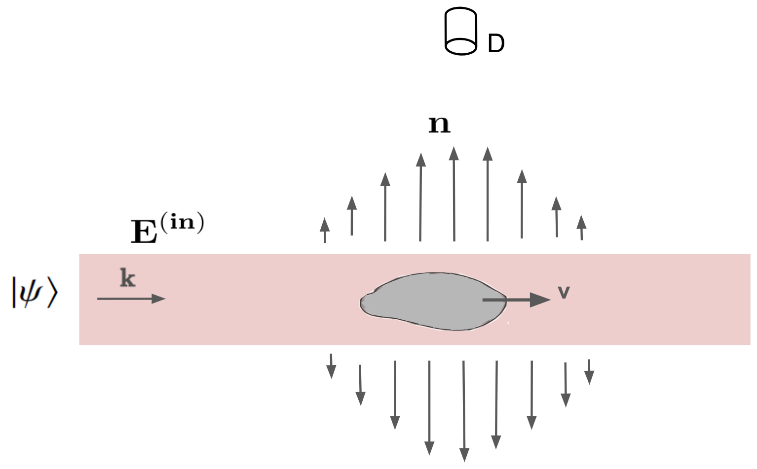
Figure 2: Scattering from dielectric moving with speed $v$. The scattered field is cylindrical; see Fig. 1 for other notations.

To understand our results, it suffices to work within the first-order Born approximation, where the scattered field $\mathbf{E}^{[\text{s}]}[\omega,\mathbf{r}]$ is determined via taking the Fourier transform (6) of (2), and assuming that $\bar{\varepsilon}{E}_{\alpha}^{[\text{s}]}$ is small:

$$\{\partial_{\beta}\partial_{\beta}-\partial_{\alpha}\partial_{\beta}+\omega^{2}\}E_{\alpha}^{[\text{s}]}[\omega,\mathbf{r}]$$ (11)

$$=-\omega^{2}\int{\rm d}\omega^{\prime}\bar{\varepsilon}(\omega-\omega^{\prime},\mathbf{r})E_{\alpha}^{[\text{in}]}[\omega^{\prime},\mathbf{r}],$$ (12)

$$E_{\alpha}^{[\text{s}]}(\omega,\mathbf{r})=-\omega^{2}\int{\rm d}\mathbf{r}^{\prime}\int{\rm d}\omega^{\prime}\times$$

$$G_{\alpha\beta}[\omega,\mathbf{r}-\mathbf{r}^{\prime}]\,\bar{\varepsilon}[\omega-\omega^{\prime},\mathbf{r}^{\prime}]\,E_{\beta}^{[\text{in}]}[\omega^{\prime},\mathbf{r}^{\prime}],$$ (13)

where $\bar{\varepsilon}[\omega,\mathbf{r}]$ is the Fourier transform of $\bar{\varepsilon}(t,\mathbf{r})$ [cf. (6)], and $G_{\alpha\beta}[\omega,\mathbf{r}]$ is retarded Green’s function of Helmholtz’s operator [see sec. I of Supplementary Material (SM)]:

$$\{(\partial_{\sigma}\partial_{\sigma}+\omega^{2})\delta_{\alpha\beta}-\partial_{\alpha}\partial_{\beta}\}G_{\beta\gamma}[\omega,\mathbf{r}]=\delta_{\alpha\gamma}\delta(\mathbf{r}),$$ (14)

$$G_{\alpha\beta}[\omega>0,\mathbf{r}]=\Big{(}\delta_{\alpha\beta}+\frac{\partial_{\alpha}\partial_{\beta}}{\omega^{2}}\Big{)}\frac{e^{i\omega r}}{(-4\pi)r},~{}r=|\mathbf{r}|.$$ (15)

Eq. (13) can be related to Doppler’s effect; see sec. II of SM. For ${E}_{\alpha}^{[\text{s}]}[\omega,\mathbf{r}]$ we find from (13, A106–10):

$${E}_{\alpha}^{[\text{s}]}[\omega,\mathbf{r}]=\frac{\omega^{2}}{2i\pi}\int d\mathbf{q}\,\sqrt{q}\,[V_{\alpha\beta}[\mathbf{r,q},\omega-q]{\rm e}_{\beta\lambda}\left(\mathbf{q}\right){a}_{\lambda}\left(\mathbf{q}\right)$$

$$-V_{\alpha\beta}[\mathbf{r,-q},\omega+q]\,{\rm e}_{\beta\lambda}\left(\mathbf{q}\right){a}_{\lambda}^{\dagger}\left(\mathbf{q}\right)],$$ (16)

$$V_{\alpha\beta}[\mathbf{r,q},\omega-q]=\int d\mathbf{r}^{\prime}G_{\alpha\beta}[\omega,\mathbf{r-r}^{\prime}]\bar{\varepsilon}[\omega-q,\mathbf{r}^{\prime}]e^{i\mathbf{q\cdot r}^{\prime}}.$$

Note that for the time-independent dielectric, $\bar{\varepsilon}(\omega)\propto\delta(\omega)$, and only the annihilation operator containing part survives in (16, S33), because (S33) refers to $\omega>0$, and then $V_{\alpha\beta}[\mathbf{r,-q},\omega+q]=0$ drops out. More generally, also the creation operator will contribute to (S33), which is the core of our effects. We now apply (16, S33) to a resting, but space-time-modulated dielectric, and then show how (16, S33) describe qualitatively the moving dielectric confirming the relativistic theory for that situation developed in sec. III of SM.

Vacuum response of space-time-modulated dielectric. For simplicity, we work with the following model of space-time-modulated dielectric [see Fig. 1]:

$$\bar{\varepsilon}\left(\mathbf{r,}t\right)=\chi\left(\mathbf{r}\right)\left[1+\eta\left(x-wt\right)\right],$$ (17)

$$\bar{\varepsilon}[\omega,\mathbf{r}]=\chi(\mathbf{r})(\delta\left(\omega\right)+\frac{1}{w}\eta[-\omega/w]e^{i\omega x/w}),$$ (18)

where $\chi\left(\mathbf{r}\right)$ is a localized function that defines the overall shape of the dielectric, $\eta\left(x-wt\right)$ refers to the unknown structure along the $x$-axis that defines the modulation, and $\eta[\omega]$ is the Fourier transform of $\eta(t)$ [cf. (6)]. The modulation speed $w>0$ can be larger than $c=1$ since it does not refer to the energy or information transfer Huidobro et al. (2019); Caloz et al. (2022). However, we shall not need $w>c=1$.

We calculate the vacuum response of the photodetector starting from (S33, 16, 18) for $|\psi\rangle=|0\rangle$:

$$I[\omega,\mathbf{r};|0\rangle\langle 0|]=\frac{\omega^{4}}{w^{2}(2\pi)^{4}}\int{\rm d}\mathbf{q}\,q\,|\,\eta[{(\omega+q)}/{w}]\,|^{2}$$

$$\Big{(}\delta_{\beta\gamma}-\frac{q_{\beta}q_{\gamma}}{q^{2}}\Big{)}\zeta_{\alpha\beta}(\mathbf{q,r})\zeta^{*}_{\alpha\gamma}(\mathbf{q,r}),~{}~{}q=|\mathbf{q}|,$$ (19)

$$\zeta_{\alpha\beta}(\mathbf{q,r})=\int{\rm d}\mathbf{r}^{\prime}G_{\alpha\beta}[\omega,\mathbf{r}-\mathbf{r}^{\prime}]\chi(\mathbf{r}^{\prime})e^{\frac{i(\omega+q)x^{\prime}}{w}-i\mathbf{q\cdot r}^{\prime}},$$ (20)

where only the negative frequency ($\omega^{\prime}<0$, i.e. creation operator containing) part of $\mathbf{E}^{\rm[s]}[\omega^{\prime},\mathbf{r}^{\prime}]$ contributes into (19), while $\mathbf{E}^{\rm[in]}$ cancels out from it. If $\chi(\mathbf{r}^{\prime})$ is well-localized e.g. around $\mathbf{r}^{\prime}\simeq 0$, (20) can be simplified further assuming that the photodetector in (19) is placed far away from the dielectric. In this far-field domain $|\mathbf{r}|\gg|\mathbf{r}^{\prime}|$, the photodetector sees a spherical wave [cf. (15) and sec. I of SM],

$$G_{\alpha\beta}[\omega,\mathbf{r-r}^{\prime}]\simeq(\delta_{\alpha\beta}-n_{\alpha}n_{\beta})\frac{e^{i\omega r-i\omega\mathbf{n\cdot r^{\prime}}}}{r},~{}\mathbf{n}=\frac{\mathbf{r}}{r},$$ (21)

and (19) simplifies, since (20) reduces via (21) to the Fourier transform of $\chi(\mathbf{r})$. Note that for the finiteness of the integral in (19), $\left|\eta\left(\frac{\omega+q}{w}\right)\right|^{2}$ should decay with $q$ sufficiently quickly. For instance, if $\eta\left(x\right)$ is Gaussian in (17), $\left|\eta\left(\frac{\omega+q}{w}\right)\right|^{2}$ is also Gaussian and the integral (19) will be finite. The fact that (19, 20) essentially depends on $\left|\eta\left(\frac{\omega+q}{w}\right)\right|^{2}$ means that certain features of the susceptibility can be deduced from the vacuum response, i.e. without shining any light on the dielectric.

Vacuum response of moving dielectric. We now consider an ordinary (non-modulated) dielectric moving along the $x$-axis with a constant speed $v<c=1$; see Fig. 2. The dielectric susceptibility and its Fourier transform now read

$$\bar{\varepsilon}(\gamma(x-vt),y,z),~{}~{}\gamma=(1-v^{2})^{-1/2},$$ (22)

$$\bar{\varepsilon}[\omega,\mathbf{r}]=\frac{1}{\gamma v}e^{i\omega x/v}\bar{\varepsilon}\Big{[}-\frac{\omega}{\gamma v},y,z\Big{]},$$ (23)

where $\bar{\varepsilon}(x,y,z)$ is the susceptibility at rest. Eqs. (22, S53) imply the relativistic situation (due to $\gamma$) which we adopted for greater generality. The relativistic consideration was not needed for the modulated situation (17, 18), because the modulation speed (not limited by special relativity, since there is no energy transfer or information transfer) can be comparable to or even greater than the speed of light Huidobro et al. (2019); Caloz et al. (2022). Hence, for studying (22–S77) we need a relativistic covariant scattering theory, which we developed in sec. IV of SM based on Minkowski’s formalism Minkowski (1908). However, our main results can be qualitatively understood by using (S53) in (19, 20). Instead of (S53), we shall work with even a simpler model of a thin road

$$\bar{\varepsilon}(x,y,z)=\bar{\varepsilon}(x)\delta(\boldsymbol{\rho}),~{}~{}\bar{\varepsilon}[\omega,\mathbf{r}]=\frac{e^{i\omega x/v}}{\gamma v}\bar{\varepsilon}\Big{[}-\frac{\omega}{\gamma v}\Big{]}\delta(\boldsymbol{\rho}),$$

$$\boldsymbol{\rho}=(x_{1},x_{2})=(y,z),~{}~{}\rho=|\boldsymbol{\rho}|.$$ (24)

We find from (19, 20, S77):

$$\widetilde{I}[\omega,\rho;|0\rangle\langle 0|]=\frac{\omega^{4}}{v^{2}\gamma^{2}(2\pi)^{4}}\int{\rm d}\mathbf{q}\,q\,\Big{|}\bar{\varepsilon}\Big{[}\frac{\omega+q}{v\gamma}\Big{]}\Big{|}^{2}$$

$$\Big{(}\delta_{\beta\gamma}-\frac{q_{\beta}q_{\gamma}}{q^{2}}\Big{)}\zeta_{\alpha\beta}(\mathbf{q},\rho)\zeta^{*}_{\alpha\gamma}(\mathbf{q},\rho),$$ (25)

$$\zeta_{\alpha\beta}(\mathbf{q},\rho)=-\frac{1}{2\pi}(\delta_{\alpha\beta}-\frac{\partial_{\alpha}\partial_{\beta}}{\omega^{2}})K_{0}(\rho\sqrt{b^{2}-\omega^{2}}\,),$$ (26)

where $b\equiv\frac{\omega+q}{v}-{q_{1}}$ and $K_{0}$ is Bessel’s $K_{0}$-function. Eq. (26) is deduced in sec. III of SM. Note that $b>\omega>0$ due to $v<1$, i.e. $K_{0}$ in (26) is real.

Since $\widetilde{I}$ in (Enhanced detection of time-dependent dielectric structure: Rayleigh’s limit and quantum vacuum, 26) depends on $\rho$ only, it refers to cylindrical waves. This is due to the thin-road model (S77) and the anisotropy introduced by the motion along the $x$-axis. The spherical far-field limit (21) does not apply to the moving dielectric e.g. because $|\bar{\varepsilon}[\omega,\mathbf{r}]|^{2}$ in (S53) does not depend on $x$, and hence does not nullify for $x\to\pm\infty$. The known asymptotics

$$K_{0}(x\gg 1)\simeq e^{-x}\,\sqrt{{\pi}/{(2x)}},$$ (27)

means that the integral in (Enhanced detection of time-dependent dielectric structure: Rayleigh’s limit and quantum vacuum) is finite even if $|\bar{\varepsilon}[{(\omega+q)}/{v}]|^{2}$ is non-zero for $q\to\infty$, i.e. for a point-like particle. This situation differs from the modulated case (19) which did not apply to point particles, where $|\eta[{(\omega+q)}/{w}]|^{2}={\rm const}$ (the interior of such a particle cannot be modulated). Note that the vacuum effect is a consequence of the relative motion of the detector and scatterer, and it does not contradict the principle of relativity. For a point-like moving object, (Enhanced detection of time-dependent dielectric structure: Rayleigh’s limit and quantum vacuum–27) imply $\widetilde{I}={\cal O}(\rho^{-6})$ for sufficiently large $\rho$, i.e. this vacuum response does not become exponentially small far away from the particle trajectory.

One-photon incident field. We return to (16–18) and shine the modulated dielectric with a single-photon light

$$\left|\psi\right\rangle=\int d\mathbf{q}C_{\lambda}\left(\mathbf{q}\right)\hat{a}_{\lambda}^{\dagger}\left(\mathbf{q}\right)\left|0\right\rangle,~{}\int d\mathbf{q}|C_{\lambda}(\mathbf{q})|^{2}=1,$$ (28)

where $\left|0\right\rangle$ is the vacuum state of the field, and the second relation in (28) ensures $\left\langle\psi|\psi\right\rangle=1$. While the single-photon state was taken for clarity, similar results are obtained for a coherent state of the field that models laser light; see sec. IV of SM. Now the photodetector will be placed in the far-field domain; see Fig. 1. Hence, in (S33) we can take $\mathbf{E}=\mathbf{E}^{[\text{s}]}$, i.e. only the scattered field contributes; cf. (A106). Using (16) we find

$$I[\omega,\mathbf{r};|\psi\rangle\langle\psi|]=I[\omega,\mathbf{r};|0\rangle\langle 0|]+\sum_{s=\pm}\xi_{\alpha}(s)\xi^{*}_{\alpha}(s),$$

$$\xi_{\alpha}(s)=\int\frac{\sqrt{q}{\rm d}\mathbf{q}}{2\pi}C_{\lambda}\left(\mathbf{q}\right)V_{\alpha\beta}\left(\mathbf{r},s\mathbf{q},\omega-sq\right)e_{\beta\lambda}\left(\mathbf{q}\right),$$ (29)

where the vacuum contribution (19, 20) enters additively, and where $s=\pm$ comes from (resp.) positive and negative frequencies. We now assume that the single-photon state (28) has a well-defined momentum $\mathbf{k}$, i.e.

$$C_{\lambda}\left(\mathbf{q}\right)=c_{\lambda}C\left(\mathbf{q}\right),~{}C\left(\mathbf{q}\right)~{}{\rm concentrates~{}at}~{}\mathbf{q\simeq k}.$$ (30)

Using (21) in the far-field domain, we confirm that generally, all frequencies appear in (29). This contrasts with the weak scattering from a resting non-modulated dielectric, where $\mathbf{E}^{[{\rm s}]}$ contains only the incident frequency $|\mathbf{k}|$ [cf. (18)], hence the photodetector should be tuned to that frequency: $\omega\simeq|\mathbf{k}|$. The classical Rayleigh limit is a result of this fact Avetisyan et al. (2023).

For clarity, we assume $|\mathbf{k}|\not=\omega$ in (29), i.e. the detection frequency differs from the incident frequency. Together with (30), this allows us to exclude the term $\propto\delta(\omega)$ in (18). We find from (29, 30, 16):

$$I[\omega,\mathbf{r};|\psi\rangle\langle\psi|]-I[\omega,\mathbf{r};|0\rangle\langle 0|]=\frac{(2\pi)^{6}\sigma}{w^{2}r^{2}}\times$$

$$\sum_{s=\pm}\Big{|}\eta\Big{[}\frac{\omega-sk}{w}\Big{]}\,\chi\Big{[}s\mathbf{k}-\omega\mathbf{n}+\mathbf{h}_{x}\frac{\omega-sk}{w}\Big{]}\Big{|}^{2},$$ (31)

$$\sigma=(\mathbf{p\cdot p}^{*}-|\mathbf{p\cdot n}|^{2})\left|\int\frac{\sqrt{q}\,{\rm d}\mathbf{q}}{2\pi}C\left(\mathbf{q}\right)\right|^{2},$$ (32)

where $p_{\alpha}=c_{\lambda}e_{\alpha\lambda}$ is the polarization vector, $\mathbf{h}_{x}$ is the unit vector of the $x$-axis, and $\chi[\mathbf{q}]\equiv\int\frac{{\rm d}\mathbf{r}}{(2\pi)^{3}}e^{-i\mathbf{q\cdot r}}\chi(\mathbf{r})$. Note the factor $|\eta[{(\omega+k)}/{w}]|^{2}$ in (31), which comes from Doppler’s effect and negative frequencies; cf. sec. II of SM. For $w<1$, $|\eta[{(\omega+k)}/{w}]|^{2}$ shows that the susceptibility enters with its Fourier components at frequencies much larger than both $\omega$ and $k=|\mathbf{k}|$. This goes against classical Rayleigh’s limit. The validity of this limit implies that the far-field photodetection response contains only $|\eta[\omega^{\prime}]|^{2}$ with $\omega^{\prime}\simeq k$ Avetisyan et al. (2023). Note that the factor $|\eta[{(\omega-k)}/{w}]|^{2}$ can also violate Rayleigh’s limit, e.g. for $\omega=k/2$ and a sufficiently small $w$. Hence (31) with two factors $|\eta[{(\omega+sk)}/{w}]|^{2}$ ($s=\pm$) suggests a modified form of Rayleigh’s limit that contains the modulation speed $w$; see also below.

There are examples, where Rayleigh’s limit is violated for evanescent fields Novotny and Hecht (2012), but we are not aware of far-field violations of this limit besides the effects related to specific quantum correlation (entanglement) features of the incident light Shih et. al. (2001); Abouraddy et al. (2002); Boto et. al. (2000); Santos et al. (2003); Liu et al. (2021); Avetisyan et al. (2023). Here no such correlated states are needed, because violations of the classical limit occur due to the space-time modulation.

For a moving dielectric (22–S77) we get from (S77, 29, 30) for the one-photon contribution in (S33), where we deliberately include only the scattered field $\mathbf{E}^{[\text{s}]}$:

$$\widetilde{I}[\omega,\rho;|\psi\rangle\langle\psi|]-\widetilde{I}[\omega,\rho;|0\rangle\langle 0|]\sim\left|\int\frac{\sqrt{q}\,{\rm d}\mathbf{q}}{2\pi}C\left(\mathbf{q}\right)\right|^{2}\times$$

$$\sum_{s=\pm}\Big{|}\bar{\varepsilon}\Big{[}\frac{\omega+sk}{\gamma v}\Big{]}K_{0}[\rho\sqrt{b_{s}^{2}-\omega^{2}}]\Big{|}^{2},~{}~{}k=|\mathbf{k}|,$$ (33)

$$b_{s}=(\omega-sk)/v+sk_{1},~{}~{}\mathbf{k}=(k_{1},k_{2},k_{3}),$$ (34)

where $\sim$ in (33) means that some (irrelevant) contributions were omitted. Eq. (33) implies a similar conclusion (as (31) above) for the invalidity of classical Rayleigh’s limit. But there are 3 important differences. First, due to $b_{-}^{2}-\omega^{2}>0$ in (33), $K_{0}[\rho\sqrt{b_{-}^{2}-\omega^{2}}]$ is an exponentially decaying function of $\rho$ [cf. (27)], i.e. $|\bar{\varepsilon}[{(\omega+k)}/{(\gamma v)}]|^{2}$ goes beyond Rayleigh’s limit only in the near-field situation. Now both signs of $b_{+}^{2}-\omega^{2}$ are possible. For $b_{+}^{2}-\omega^{2}<0$ the corresponding $K_{0}$ function in (33) should read $K_{0}[-i\rho\sqrt{|b_{+}^{2}-\omega^{2}|}]$, which decays as a power law $\rho^{-1/2}$; cf. (27) and see sec. III of SM. However, for $b_{+}^{2}-\omega^{2}<0$ we do not see any significant detection enhancement coming from $|\bar{\varepsilon}[{(\omega-k)}/{(\gamma v)}]|^{2}$. Hence the detection enhancement implied by (33) is overall limited to near fields. Second, recall that (33) includes only $\mathbf{E}^{[\text{s}]}$. In contrast to the far-field domain, the exclusion of the incident field $\mathbf{E}^{[\text{in}]}$ in the near-field domain is not automatic. Now we need an additional, polarization-dependent filtering; see sec. IV of SM. Third, in the ultrarelativistic limit $v\to 1=c$, Rayleigh’s limit in $|\bar{\varepsilon}[{(\omega\pm k)}/{(\gamma v)}]|^{2}$ is enforced due to $1/(\gamma v)\to 0$; this is a consequence of the relativistic Fitzgerald-Lorentz contraction that hinders the determination of the dielectric’s internal structure. All these conclusions are validated in sec. IV of SM within the fully covariant theory.

In sum, we show that uniform motion or space-time modulation is a resource for detecting dielectric susceptibility. First, there is a vacuum signal that allows us to determine some features of the susceptibility without shining light on the dielectric. Second, when the incident light is there, the classical Rayleigh’s limit is modified so that the detection is enhanced.

We were supported by HESC of Armenia, grants 24FP-1F030 and 21AG-1C038. We thank R. Ghazaryan for discussions on Doppler’s effect.

SUPPLEMENTARY MATERIAL for
Enhanced detection of time-dependent dielectric structure:
Relativistic Rayleigh’s limit and quantum vacuum

This supplementary material consists of four sections. In section I we briefly comment on the Green function for Helmholtz equation. In section II we explain the relations of our results with Doppler’s effect. In section III we calculate several integrals with Bessel’s function. Based on Minkowski’s formalism, in section IV we developed a relativistically covariant scattering theory of light from a moving dielectric.

I Green’s function for the Helmholtz equation

This function is defined as follows:

$$\{(\partial_{\sigma}\partial_{\sigma}+\omega^{2})\delta_{\alpha\beta}-\partial_{\alpha}\partial_{\beta}\}G_{\beta\gamma}[\omega,\mathbf{r}]=\delta_{\beta\gamma}\delta(\mathbf{r}),$$ (S1)

$$G_{\alpha\beta}[\omega>0,\mathbf{r}]=\Big{(}\delta_{\alpha\beta}+\frac{\partial_{\alpha}\partial_{\beta}}{\omega^{2}}\Big{)}\frac{e^{i\omega r}}{(-4\pi)r},~{}r=|\mathbf{r}|,$$ (S2)

$$\partial_{\alpha}\equiv\partial/\partial x_{\alpha},~{}~{}~{}~{}\alpha,\beta=1,2,3,$$ (S3)

$$\mathbf{r}=(x_{1},x_{2},x_{3})=(x,y,z),$$ (S4)

where (S2) is found from (S1) using the known expression for the Laplace equation

$$\partial_{\sigma}\partial_{\sigma}G_{\omega}(\mathbf{r})=\delta(\mathbf{r}),~{}~{}~{}~{}~{}G_{\omega}(\mathbf{r})\equiv\frac{e^{i\omega r}}{(-4\pi)r}.$$ (S5)

Hence we get from (S2)

$$\omega^{2}G_{\alpha\beta}\left(\omega,\mathbf{r}\right)=\frac{1}{3}\delta_{\alpha\beta}\delta\left(\mathbf{r}\right)$$ (S6)

$$+\frac{e^{i\left|\omega\right|r}}{4\pi r^{3}}\Big{\{}\left[1-i\omega r-\left(\omega r\right)^{2}\right]\delta_{\alpha\beta}$$ (S7)

$$-\left[3-3i\omega r-\left(\omega r\right)^{2}\right]n_{\alpha}n_{\beta}\Big{\}},~{}~{}\mathbf{n}=\mathbf{r}/|\mathbf{r}|.$$ (S8)

In the far field limit $\omega r\gg 1$ we get:

$$G_{\alpha\beta}\left(\omega,\mathbf{r}\right)\rightarrow G_{\omega}\left(\mathbf{r}\right)\left(\delta_{\alpha\beta}-n_{\alpha}n_{\beta}\right),$$ (S9)

while in the near field limit $\omega r\ll 1$ we have

$$\omega^{2}G_{\alpha\beta}\left(\omega,\mathbf{r}\right)\rightarrow\frac{1}{3}\delta_{\alpha\beta}\delta\left(\mathbf{r}\right)+\frac{1}{4\pi r^{3}}\left(\delta_{\alpha\beta}-3n_{\alpha}n_{\beta}\right).$$

II Relations with Doppler physics

In the main text, we found the following relation for the scattered field

$$E_{\alpha}^{[\text{s}]}(\omega,\mathbf{r})=-\omega^{2}\int{\rm d}\mathbf{r}^{\prime}\int{\rm d}\omega^{\prime}\times$$

$$G_{\alpha\beta}[\omega,\mathbf{r}-\mathbf{r}^{\prime}]\,\bar{\varepsilon}[\omega-\omega^{\prime},\mathbf{r}^{\prime}]\,E_{\beta}^{[\text{in}]}[\omega^{\prime},\mathbf{r}^{\prime}].$$ (S10)

Our purpose is to show that this equation directly relates to the Doppler physics. Recall that

$$\bar{\varepsilon}[\omega,\mathbf{r}]=\int\frac{{\rm d}t}{2\pi}e^{it\omega}\bar{\varepsilon}(t,\mathbf{r}).$$ (S11)

For $\bar{\varepsilon}(t,\mathbf{r})$ we select the following simple model of moving non-relativistic dielectric

$$\bar{\varepsilon}(t,\mathbf{r})=\bar{\varepsilon}(\mathbf{r}-\mathbf{v}t),$$ (S12)

where $\mathbf{v}$ is the constant velocity of motion, and where for the space-Fourier transform $\hat{\varepsilon}[\mathbf{k}]$ of the static susceptibility $\bar{\varepsilon}(\mathbf{r})$ we have

$$\bar{\varepsilon}(\mathbf{r})=\int{\rm d}\mathbf{k}\,e^{i\mathbf{k\cdot r}}\,\hat{\varepsilon}[\mathbf{k}].$$ (S13)

Now (S10–S13) imply

$$E_{\alpha}^{[\text{s}]}(\omega,\mathbf{r})=-\omega^{2}\int{\rm d}\mathbf{r}^{\prime}\int{\rm d}{\mathbf{k}}\hat{\varepsilon}[\mathbf{k}]e^{\mathbf{k\cdot r}^{\prime}}\,\times$$

$$G_{\alpha\beta}[\omega,\mathbf{r}-\mathbf{r}^{\prime}]\,E_{\beta}^{[\text{in}]}[\omega-\mathbf{k\cdot v},\mathbf{r}^{\prime}].$$ (S14)

Note that the factor $E_{\beta}^{[\text{in}]}[\omega-\mathbf{k\cdot v},\mathbf{r}^{\prime}]$ in (S14) has the Doppler-shifted frequency $\omega-\mathbf{k\cdot v}$.

Let us now assume that

– The incident field $E_{\beta}^{[\text{in}]}[\omega-\mathbf{k\cdot v},\mathbf{r}^{\prime}]$ is classical and concentrated at a frequency $\omega_{0}>0$.

– The motion is along the $x$-axis: $\mathbf{k\cdot v}=k_{x}v$.

– $\hat{\varepsilon}[k_{x},k_{y},k_{z}]$ is weakly dependent on $k_{y}$ and $k_{z}$ (i.e. the moving dielectric is a thin road).

These assumptions produce from (S14):

$$E_{\alpha}^{[\text{s}]}(\omega,\mathbf{r})\propto\hat{\varepsilon}\Big{[}\frac{\omega-\omega_{0}}{v}\Big{]}.$$ (S15)

III Calculation of Bessel integrals

We explain how to calculate the following integral

$$\int\frac{{\rm d}x}{(-4\pi)}\,\frac{e^{i\omega\sqrt{x^{2}+\rho^{2}}+ix(\frac{\omega+q}{v}-q^{1})}}{\sqrt{x^{2}+\rho^{2}}},$$ (S16)

$$\rho=\sqrt{(y^{1})^{2}+(y^{2})^{2}},\quad b=\frac{\omega+q}{v}-q^{1},$$ (S17)

which appears in (S79) below and also in Eq. (25) of the main text.

We employ the known Fourier representation:

$$-\frac{1}{4\pi|\boldsymbol{x}|}\,e^{i|\boldsymbol{x}|\,|\omega|}=\int\frac{{\rm d}^{3}q}{(2\pi)^{3}}\frac{e^{i\boldsymbol{q}\boldsymbol{x}}}{\omega^{2}+i0-q^{2}},$$ (S18)

and find

$$(\ref{bull1})=-\int\frac{{\rm d}^{2}q}{(2\pi)^{2}}\frac{e^{iq^{2}x^{2}+iq^{3}x^{3}}}{q^{2}+b^{2}-\omega^{2}-i0}$$ (S19)

$$=-\int_{0}^{\infty}\frac{q{\rm d}q}{2\pi}\frac{J_{0}(q\rho)}{q^{2}+b^{2}-\omega^{2}-i0}$$ (S20)

$$=-\frac{1}{2\pi}K_{0}(\rho\sqrt{b^{2}-\omega^{2}}),$$ (S21)

where we employed for Bessel’s $J$-function:

$$J_{0}(x)=\int_{0}^{2\pi}\frac{{\rm d}\theta}{2\pi}{e^{ix\cos\theta}},$$ (S22)

and where the transition from (S20) to (S21) is a tabulated formula that holds for

$$b^{2}-\omega^{2}>0.$$ (S23)

For $b$ defined via (S17), condition (S23) is valid due to $v<1$. In particular, (S23) ensures that $i0$ in (S20) can be get rid of.

A simpler and more direct way to obtain (S21) under condition (S23) is to start from (S19), employ there

$$\frac{1}{q^{2}+b^{2}-\omega^{2}}=\int_{0}^{\infty}{\rm d}s\,e^{-s(q^{2}+b^{2}-\omega^{2})},$$ (S24)

take the resulting Gaussian integrals and after a change of variables to arrive at (S21) with an alternative representation of Bessel’s $K$-function:

$$K_{0}(x)=\int_{1}^{\infty}{\rm d}t\,\frac{e^{-tx}}{\sqrt{t^{2}-1}}.$$ (S25)

Now (S25) relates to a more standard representation of $K_{0}$

$$K_{0}(x)=\frac{1}{2}\int{\rm d}t\,\frac{e^{itx}}{\sqrt{1+t^{2}}},$$ (S26)

via going to the complex plane.

Recall the asymptotic expansions of $K_{0}(x)$ (for $x>0$) that are deduced from (S25):

$$K_{0}(x)=\ln\Big{[}\frac{2e^{-\gamma_{\rm Euler}}}{x}\Big{]}+{\cal O}(x^{2}\ln x),~{}~{}x\to 0$$ (S27)

$$K_{0}(x)=\sqrt{\frac{\pi}{2x}}e^{-x}\Big{[}1-\frac{1}{8x}+{\cal O}(x^{-2})\Big{]},~{}~{}x\gg 1.$$ (S28)

If (S23) does not hold, we need to understand how to make the analytical continuation in (S21). This is achieved from (S20) upon using Sokhotsky’s formula:

$$\frac{1}{x-i0}={\rm v.p.}\frac{1}{x}+i\pi\delta(0).$$ (S29)

Again using tabulated formulas for Bessel’s function we obtain that when (S23) does not hold:

$$(\ref{goncho})=-\frac{1}{2\pi}K_{0}(-i\rho\sqrt{|b^{2}-\omega^{2}|})$$ (S30)

$$=\frac{1}{4i}H^{[1]}_{0}(\rho\sqrt{|b^{2}-\omega^{2}|}).$$ (S31)

Recall that

$$H^{[1]}_{0}(x)\simeq\sqrt{\frac{2}{x\pi}}\,e^{i(x-\frac{\pi}{4})},~{}~{}x\gg 1.$$ (S32)

IV Wave-equation for moving dielectric: Relativistic formalism

Notations: Latin and Greek ($\sigma$, $\mu$, $\nu$,..) indices assume (resp.) values $0,1,2,3$ and $1,2,3$ and refer (resp.) to 4-vectors and 3-vectors. Greek indices $\alpha$ and $\beta$ refer to polarization of light. We set $g_{ik}={\rm diag}[1,-1,-1,-1]$ and $c=1$. 3-vectors are denoted as $\boldsymbol{x}=(x^{1},x^{2},x^{3})$.

Consider a dielectric which in the laboratory frame moves along $x^{1}$-axes with a constant velocity $v$. The electromagnetic field tensor $F^{ik}$ holds the following wave-equation Minkowski (1908); Pal (2021) (see Appendix A for derivation)

$$-\partial_{i}F^{ik}=\partial_{i}\Big{[}\bar{\varepsilon}(F^{is}u_{s}u^{k}-F^{ks}u_{s}u^{i})\Big{]},~{}\bar{\varepsilon}=\varepsilon-1,$$ (S33)

$$F^{ik}=\partial^{i}A^{k}-\partial^{k}A^{i},\quad x^{i}=(t,\boldsymbol{x}),$$ (S34)

$$u^{i}=\gamma(1,v,0,0),\quad\gamma\equiv(1-v^{2})^{-1/2},\,u_{i}u^{i}=1,$$ (S35)

where $A^{i}$ is the 4-potential, $u^{i}$ is the 4-velocity, and $\varepsilon(x^{i})$ is a scalar field standing for the dielectric permeability; i.e. $\varepsilon-1$ is the susceptibility. In the rest-frame $\varepsilon(x^{\prime i})$ holds the standard definition; see Appendix A. We work out (S33) via the Lorenz gauge Landau and Lifshitz (1975):

$$\partial_{i}A^{i}=0.$$ (S36)

The purpose of (S36) is to get the d’Alembert operator $-\partial_{i}\partial^{i}$ in the LHS of (S33):

$$-\partial_{i}\partial^{i}A^{k}=\partial_{i}\Big{[}\bar{\varepsilon}\Big{(}\partial^{i}Au^{k}-\partial^{k}Au^{i}$$

$$\qquad\qquad\qquad+\partial\Big{(}A^{k}u^{i}-A^{i}u^{k}\Big{)}\Big{)}\Big{]},$$ (S37)

$$\partial\equiv u^{s}\partial_{s},\qquad A\equiv A^{i}u_{i}.$$ (S38)

Eqs. (S33, S38) apply to any scalar permeability $\varepsilon(x^{i})$. Note that $u^{i}=\delta^{i}_{0}$ for $v\to 0$, where we find from (S33):

$$-\partial_{i}\partial^{i}A^{0}=\partial_{\beta}\Big{[}\bar{\varepsilon}E^{\beta}\Big{]},$$ (S39)

$$-\partial_{i}\partial^{i}A^{\sigma}=-\partial_{0}\Big{[}\bar{\varepsilon}E^{\sigma}\Big{]},~{}~{}E^{\sigma}=\partial^{\sigma}A^{0}-\partial^{0}A^{\sigma},$$ (S40)

where $E^{\sigma}$ is the electric field.

We now assume that $\varepsilon$ is time-independent in its rest-frame. In the considered laboratory frame we get [cf. (S35)]:

$$\bar{\varepsilon}=\bar{\varepsilon}[\gamma(x-vt),y,z],\quad u^{s}\partial_{s}\bar{\varepsilon}=0.$$ (S41)

This is the minimal model for a finite dielectric placed in the vacuum. Using (S41) in (S37) we get:

$$-\partial_{i}\partial^{i}A^{k}=\bar{\varepsilon}(u^{k}\partial_{i}\partial^{i}A-\partial\partial^{k}A+\partial^{2}A^{k})$$

$$+u^{k}(\partial_{i}\bar{\varepsilon})(\partial^{i}A-\partial A^{i}).$$ (S42)

IV.1 Scattering

For developing a scattering theory based on (S42), we decompose

$$A_{k}=A_{k}^{\rm[in]}+A_{k}^{\rm[s]},\qquad\partial_{i}\partial^{i}A_{k}^{\rm[in]}=0.$$ (S43)

We assume that $\bar{\varepsilon}$ is small. In the first order of Born’s perturbation theory we get from (S42, S43):

$$-\partial_{i}\partial^{i}A^{{\rm[s]}\,k}(t,\boldsymbol{x})=\Phi^{k}(t,\boldsymbol{x}),$$ (S44)

$$\Phi^{k}\equiv\bar{\varepsilon}(-\partial\partial^{k}A^{\rm[in]}+\partial\partial A^{{\rm[in]}\,k})$$

$$+u^{k}(\partial_{i}\bar{\varepsilon})(\partial^{i}A^{\rm[in]}-\partial A^{{\rm[in]}\,i}).$$ (S45)

We assume that the incident free field $A_{i}^{\rm in}$ (in contrast to scattered $A_{i}^{\rm s}$) holds Coulomb gauge conditions that imply (S36):

$$A^{{\rm[in]}\,0}=0,\qquad\partial_{\sigma}A^{{\rm[in]}\,\sigma}\equiv{\rm div}\boldsymbol{A}^{\rm[in]}=0,$$ (S46)

where $\sigma=1,2,3$.

The scattered electric field $E^{\sigma}=\partial^{\sigma}A^{0}-\partial^{0}A^{\sigma}$ reads from (S44)

$$-\partial_{i}\partial^{i}E^{{\rm[s]}\,\sigma}(t,\boldsymbol{x})=-\partial_{\sigma}\Phi^{0}-\partial_{t}\Phi^{\sigma}.$$ (S47)

IV.1.1 Incident and scattered fields

Define the Fourier transformations over time and coordinate as follows

$$A(t)=\int{\rm d}\omega\,e^{-it\omega}A(\omega),$$ (S48)

$$A(\omega)=\int\frac{{\rm d}t}{2\pi}\,e^{it\omega}A(t),$$ (S49)

$$A(\boldsymbol{x})=\int{\rm d}^{3}q\,e^{i\boldsymbol{x}\boldsymbol{q}}A(\boldsymbol{q}),$$ (S50)

$$A(\boldsymbol{q})=\int\frac{{\rm d}^{3}x}{(2\pi)^{3}}\,e^{-i\boldsymbol{x}\boldsymbol{q}}A(\boldsymbol{x}).$$ (S51)

Hence we get

$$\bar{\varepsilon}(\omega,\boldsymbol{x})=\int\frac{{\rm d}t}{2\pi}\,e^{it\omega}\bar{\varepsilon}(\gamma(x-vt),y,z)$$ (S52)

$$=\frac{1}{\gamma v}e^{i\omega x/v}\bar{\varepsilon}\Big{[}\frac{\omega}{\gamma v},y,z\Big{]},$$ (S53)

where the $\bar{\varepsilon}\Big{[}\frac{\omega}{\gamma v},y,z\Big{]}$ is the Fourier transform over the first coordinate only [cf. (S50)] taken at $\frac{\omega}{\gamma v}$.

Note that there is an important difference between a time-independent $\bar{\varepsilon}(t,\boldsymbol{x})=\bar{\varepsilon}(\boldsymbol{x})$ that is localized in all space directions and (S53), which is not localized along the $x$-axes. Indeed, note that $|\bar{\varepsilon}(\omega,\boldsymbol{x})|^{2}$ in (S53) does not depend on $x$. In particular, this fact means that taking the far-field limit for the scattered field cannot proceed along the standard lines that work for a $\bar{\varepsilon}(t,\boldsymbol{x})=\bar{\varepsilon}(\boldsymbol{x})$ that is localized along all space directions.

The above reasoning does not contradict to the fact that for $v\to 0$ we get from (S53):

$$\bar{\varepsilon}(\omega,\boldsymbol{x})=\delta(\omega)\bar{\varepsilon}(\boldsymbol{x}),~{}~{}{\rm for}~{}~{}v\to 0.$$ (S54)

Indeed, we face here a non-commutativity of two limiting processes: $v\to 0$ and $x\to\infty$, which is explicitly employed in the far-field limit.

Eq. (S44) can be written as

$$(\Delta+\omega^{2})A^{{\rm[s]}\,k}(\omega,\boldsymbol{x})=\Phi^{k}(\omega,\boldsymbol{x}),$$ (S55)

where $A^{{\rm[s]}\,k}(\omega,\boldsymbol{x})$ results from a partial (time-only) Fourier transform; see (S48, S49).

The incident (free) quantum field amounts to the following Heisenberg operators:

$$A^{i}(t,\boldsymbol{x})=\int{\rm d}^{3}q\,e^{i\boldsymbol{q}\cdot\boldsymbol{x}-i|\boldsymbol{q}|t}\,\frac{i\chi^{i}_{\alpha}(\boldsymbol{q})a_{\alpha}(\boldsymbol{q})}{2\pi\sqrt{|\boldsymbol{q}|}}+{\rm h.c.},$$ (S56)

$$\chi^{0}_{\alpha}(\boldsymbol{q})=0,\quad\chi^{\sigma}_{\alpha}(\boldsymbol{q})q^{\sigma}=0,\quad\alpha,\,\beta=1,2,$$ (S57)

$${\chi}^{\sigma}_{\alpha}(\boldsymbol{q}){\chi}^{\sigma}_{\beta}(\boldsymbol{q})=\delta_{\alpha\beta},$$ (S58)

$$A^{i}(\omega,\boldsymbol{x})=\oint\displaylimits_{|\boldsymbol{m}|=1}{\rm d}m\,e^{i\omega\boldsymbol{m}\cdot\boldsymbol{x}}\,\frac{i|\omega|^{3/2}\chi^{i}_{\alpha}(\boldsymbol{m})b_{\alpha}(|\omega|\boldsymbol{m},\omega)}{4\pi^{2}}$$ (S59)

$$b_{\alpha}(|\omega|\boldsymbol{m},\omega)=a_{\alpha}(\omega\boldsymbol{m})~{}~{}{\rm for}~{}~{}\omega>0,$$ (S60)

$$b_{\alpha}(|\omega|\boldsymbol{m},\omega)=-a^{\dagger}_{\alpha}(|\omega|\boldsymbol{m})~{}~{}{\rm for}~{}~{}\omega<0,$$ (S61)

$$a_{\alpha}(\boldsymbol{q}_{2})a^{\dagger}_{\beta}(\boldsymbol{q}_{1})-a^{\dagger}_{\beta}(\boldsymbol{q}_{1})a_{\alpha}(\boldsymbol{q}_{2})=\delta_{\alpha\beta}\delta(\boldsymbol{q}_{1}-\boldsymbol{q}_{2}),$$ (S62)

where $a_{\alpha}(\boldsymbol{q}_{2})$ is the mode annihilation operator, and where the angular integral $\oint_{|\boldsymbol{m}|=1}{\rm d}m$ comes from fractioning 3d integral:

$$\oint_{|\boldsymbol{m}|=1}{\rm d}m\,\int{\rm d}r\,r^{2}f(\boldsymbol{m},r)=\int{\rm d}^{3}x\,f(\boldsymbol{x}).$$ (S63)

Note that the normalization in (S56) is chosen such that

$$\int\frac{{\rm d}^{3}x}{8\pi}(\dot{\boldsymbol{A}}^{2}(t,\boldsymbol{x})+[\boldsymbol{\nabla}\times\boldsymbol{A}(t,\boldsymbol{x})]^{2}])$$ (S64)

$$=\int{\rm d}^{3}q\,qa^{\dagger}_{\beta}(\boldsymbol{q})a_{\beta}(\boldsymbol{q})+...,$$ (S65)

where we employed (S62), and where in (S65) we omitted a factor $\propto\delta(0)$.

IV.1.2 Photodetection and Fourier representation of the scattered field

Electric fields in quantum optics are standardly measured via photodetection Garrison and Chiao (2008). A single photodetector is localized around a certain position $\boldsymbol{x}$, works at an atomic transition frequency $\omega$, and measures e.g. the mean electric field intensity

$$\langle\psi|E^{\mu\,\dagger}(\omega,\boldsymbol{x})E^{\nu}(\omega,\boldsymbol{x})|\psi\rangle,$$ (S66)

where $|\psi\rangle$ is the quantum state of the field, and where the electric field $\boldsymbol{E}(\omega,\boldsymbol{x})$ is given by (S47). Instead of (S66) we shall study a technically simpler, scattered field mean intensity

$$\langle\psi|A^{{\rm[s]}\,2\,\dagger}(\omega,\boldsymbol{x})A^{{\rm[s]}\,2}(\omega,\boldsymbol{x})|\psi\rangle,$$ (S67)

that shows the same effects as (S66).

Consider (S45, S55) for $k=2$, where the last factor in (S45) does not contribute. We get

$$A^{{\rm[s]}\,2}(\omega,\boldsymbol{y})=\int{\rm d}^{3}xG(\omega,\boldsymbol{y}-\boldsymbol{x})\int{\rm d}\hat{\omega}\,\bar{\varepsilon}(\omega-\hat{\omega},\boldsymbol{x})$$

$$(-\partial\partial^{2}A^{\rm[in]}+\partial\partial A^{{\rm[in]}\,2})(\hat{\omega},\boldsymbol{x}),$$ (S68)

where $\bar{\varepsilon}(\omega-\hat{\omega},\boldsymbol{x})$ is defined via (S53), $A^{\rm[in]}(\hat{\omega},\boldsymbol{x})$ is defined via (S38, S59), $A^{{\rm[in]}\,2}(\hat{\omega},\boldsymbol{x})$ is defined via (S59), and retarded Green’s function reads:

$$G(\omega,\boldsymbol{x})=-\frac{1}{4\pi|\boldsymbol{x}|}\,e^{i|\boldsymbol{x}|\,|\omega|}.$$ (S69)

It is clear from (S59) that in (S68) we should replace

$$\partial_{t}\to-i\hat{\omega},\qquad\partial_{\sigma}\to i\hat{\omega}m^{\sigma}.$$ (S70)

We have from (S38, S46):

$$A=-\gamma vA^{1},\qquad\partial\to-i\hat{\omega}\gamma(1-vm^{1}).$$ (S71)

Hence (S68) reads

$$A^{{\rm[s]}\,2}(\omega,\boldsymbol{y})=-\frac{i\gamma^{2}}{4\pi^{2}}\int{\rm d}\hat{\omega}\oint{\rm d}\boldsymbol{m}\,\nu(\boldsymbol{y},\boldsymbol{m}\hat{\omega},\omega-\hat{\omega})\times$$

$$|\hat{\omega}|^{7/2}(1-vm^{1})(vm^{2}\chi^{1}_{\alpha}(\boldsymbol{m})+(1-vm^{1})\chi^{2}_{\alpha}(\boldsymbol{m}))\times$$

$$b_{\alpha}(|\hat{\omega}|\boldsymbol{m},\hat{\omega}),$$ (S72)

$$\nu(\boldsymbol{y},\boldsymbol{m}\hat{\omega},\omega-\hat{\omega})$$

$$=\int{\rm d}^{3}xG(\omega,\boldsymbol{y}-\boldsymbol{x})\bar{\varepsilon}(\omega-\hat{\omega},\boldsymbol{x})e^{i\hat{\omega}\boldsymbol{m}\boldsymbol{x}}.$$ (S73)

Using (S60, S61) we employ $\int{\rm d}\hat{\omega}=\int_{0}^{\infty}{\rm d}\hat{\omega}+\int_{-\infty}^{0}{\rm d}\hat{\omega}$ and write (S72) as

$$A^{{\rm[s]}\,2}(\omega,\boldsymbol{y})=\int{\rm d}^{3}q\,\Big{[}\Theta^{(+)}_{\alpha}(\boldsymbol{q},\omega,\boldsymbol{y})a_{\alpha}(\boldsymbol{q})$$

$$-\Theta^{(-)}_{\alpha}(\boldsymbol{q},\omega,\boldsymbol{y})a^{\dagger}_{\alpha}(\boldsymbol{q})\Big{]},$$ (S74)

$$\Theta^{(+)}_{\alpha}(\boldsymbol{q},\omega,\boldsymbol{y})=-\frac{i\gamma^{2}}{4\pi^{2}}\nu(\boldsymbol{y},\boldsymbol{q},\omega-q)q^{3/2}\times$$

$$(1-vm^{1})(vm^{2}\chi^{1}_{\alpha}(\boldsymbol{m})+(1-vm^{1})\chi^{2}_{\alpha}(\boldsymbol{m})),$$ (S75)

$$\Theta^{(-)}_{\alpha}(\boldsymbol{q},\omega,\boldsymbol{y})=-\frac{i\gamma^{2}}{4\pi^{2}}\nu(\boldsymbol{y},-\boldsymbol{q},\omega+q)q^{3/2}\times$$

$$(1-vm^{1})(vm^{2}\chi^{1}_{\alpha}(\boldsymbol{m})+(1-vm^{1})\chi^{2}_{\alpha}(\boldsymbol{m})),$$ (S76)

where $q=|\boldsymbol{q}|$, and $\boldsymbol{m}$ in (S75, S76) means $\boldsymbol{m}=\boldsymbol{q}/|\boldsymbol{q}|$. It is seen that $\Theta^{(+)}_{\alpha}(\boldsymbol{q},\omega,\boldsymbol{y})$ and $\Theta^{(-)}_{\alpha}(\boldsymbol{q},\omega,\boldsymbol{y})$ refer to (resp.) positive and negative frequencies in (S72).

IV.1.3 A model for scatterer: thin road

To evaluate (S75, S76) we adopt the following model for $\bar{\varepsilon}(x^{1},x^{2},x^{3})$

$$\bar{\varepsilon}(x^{1},x^{2},x^{3})=\bar{\varepsilon}(x^{1})\delta(x^{2})\delta(x^{3}),$$ (S77)

$$\bar{\varepsilon}(\omega,x^{1},x^{2},x^{3})=\frac{1}{\gamma v}e^{i\omega x^{1}/v}\bar{\varepsilon}\Big{[}\frac{\omega}{\gamma v}\Big{]}\delta(x^{2})\delta(x^{3}),$$ (S78)

where $\bar{\varepsilon}\Big{[}\frac{\omega}{\gamma v}\Big{]}$ is the space-Fourier transform along $x^{1}$-axis; see (S48, S49). Eq. (S77) leads to [see section III for details]:

$$\nu(\boldsymbol{y},-\boldsymbol{q},\omega+q)=\frac{1}{(-4\pi)\gamma v}e^{iy^{1}(\frac{\omega+q}{v}-q^{1})}\bar{\varepsilon}\Big{[}\frac{\omega+q}{\gamma v}\Big{]}\times$$

$$\int{\rm d}x\,\frac{e^{i\omega\sqrt{x^{2}+\rho^{2}}+ix(\frac{\omega+q}{v}-q^{1})}}{\sqrt{x^{2}+\rho^{2}}}$$ (S79)

$$=\frac{1}{(-2\pi)\gamma v}e^{iy^{1}(\frac{\omega+q}{v}-q^{1})}\bar{\varepsilon}\Big{[}\frac{\omega+q}{\gamma v}\Big{]}\times$$

$$K_{0}\Big{[}\rho\sqrt{\Big{(}\frac{\omega+q}{v}-q^{1}\Big{)}^{2}-\omega^{2}}\Big{]},$$ (S80)

$$\rho=\sqrt{(y^{1})^{2}+(y^{2})^{2}},$$ (S81)

where $K_{0}[.]$ is the corresponding Bessel’s function. Eq. (S80) extendens for $\nu(\boldsymbol{y},\boldsymbol{q},\omega-q)$, but note that in (S80) we got $\sqrt{\Big{(}\frac{\omega+q}{v}-q^{1}\Big{)}^{2}-\omega^{2}}>0$, since $v<1$. In contrast, for $\nu(\boldsymbol{y},\boldsymbol{q},\omega-q)$, $\sqrt{\Big{(}\frac{\omega-q}{v}+q^{1}\Big{)}^{2}-\omega^{2}}$ may be imaginary, and if it is imaginary we should employ the analog of (S80) with [see section III for details]:

$$\nu(\boldsymbol{y},\boldsymbol{q},\omega-q)=\frac{1}{(-2\pi)\gamma v}e^{iy^{1}(\frac{\omega-q}{v}+q^{1})}\bar{\varepsilon}\Big{[}\frac{\omega-q}{\gamma v}\Big{]}\times$$

$$K_{0}\Big{[}\rho\sqrt{\Big{(}\frac{\omega-q}{v}+q^{1}\Big{)}^{2}-\omega^{2}}\Big{]},~{}~{}~{}\Big{(}\frac{\omega-q}{v}+q^{1}\Big{)}^{2}\geq\omega^{2},$$ (S82)

$$\nu(\boldsymbol{y},\boldsymbol{q},\omega-q)=\frac{1}{(-2\pi)\gamma v}e^{iy^{1}(\frac{\omega-q}{v}+q^{1})}\bar{\varepsilon}\Big{[}\frac{\omega-q}{\gamma v}\Big{]}\times$$

$$K_{0}\Big{[}-i\rho\sqrt{\omega^{2}-\Big{(}\frac{\omega-q}{v}+q^{1}\Big{)}^{2}}\Big{]},~{}~{}\Big{(}\frac{\omega-q}{v}+q^{1}\Big{)}^{2}\leq\omega^{2},$$ (S83)

where $K_{0}[-ix]=\frac{i\pi}{2}H^{[1]}_{0}[x]$. Note the asymptotic expansions:

$$K_{0}(x)=\sqrt{\frac{\pi}{2x}}e^{-x}\Big{[}1+{\cal O}(x^{-1})\Big{]},~{}~{}x\gg 1,$$ (S84)

$$K_{0}(-ix)=\sqrt{\frac{\pi}{2x}}e^{i(x+\pi/4)}\Big{[}1+{\cal O}(x^{-1})\Big{]},~{}~{}x\gg 1.$$ (S85)

IV.2 Vacuum-state intensity

We now consider a vacuum-state intensity [cf. (S67)]

$$\langle 0|A^{{\rm[s]}\,2\,\dagger}(\omega,\boldsymbol{y})A^{{\rm[s]}\,2}(\omega,\boldsymbol{y})|0\rangle,\qquad\omega>0,$$ (S86)

where $\omega>0$ is an essential requirement of the photodetection theory. It should be clear from (S62) that only $\hat{\omega}<0$ in (S72) contributes into (S86):

$$\langle 0|A^{{\rm[s]}\,2\,\dagger}(\omega,\boldsymbol{y})A^{{\rm[s]}\,2}(\omega,\boldsymbol{y})|0\rangle$$

$$=\int{\rm d}^{3}q\,\Theta^{(-)}_{\alpha}(\boldsymbol{q},\omega,\boldsymbol{y})\Theta^{(-)*}_{\alpha}(\boldsymbol{q},\omega,\boldsymbol{y})$$ (S87)

$$=\frac{\gamma^{4}}{16\pi^{4}}\int{\rm d}^{3}q\,q^{3}|\nu(\boldsymbol{y},-\boldsymbol{q},\omega+q)|^{2}$$

$$(1-vm^{1})^{2}(v^{2}(m^{2})^{2}+(1-vm^{1})^{2}),$$ (S88)

where $q=|\boldsymbol{q}|$, $\boldsymbol{m}=\boldsymbol{q}/|\boldsymbol{q}|$, and where we used (S62, S58).

We draw the following conclusions from (S88, S79).

– Eq. (S80) shows that for $v\to 0$ the correlator (S88) disappears, as it should. In this limit, $\frac{1}{\gamma v}\bar{\varepsilon}\Big{[}\frac{\omega+q}{\gamma v},y,z\Big{]}\simeq\delta(\omega+q)$, and since the integration in (S88) involves only $q>0$ (recall that $\omega>0$), the whole integral disappears.

– Eq. (S88) that contains $|\nu(\boldsymbol{y},-\boldsymbol{q},\omega+q)|^{2}$ from (S80) is invariant with respect to $v\to-v$, as expected from a vacuum contribution. Indeed, $v\to-v$ can be accompanied by $\boldsymbol{q}\to-\boldsymbol{q}$ in the integral in (S88). Now note that the integral in (S80) is an even function of $(\frac{\omega+q}{v}-q^{1})$.

– Eq. (S88) does not depend on $y^{1}$, and it depends on $y^{2}$ and $y^{3}$ only via $\rho$. This is due to the cylindrical symmetry inherent in (S77).

– Eq. (S88) is finite for all reasonable $\Big{|}\bar{\varepsilon}\Big{[}\frac{\omega+q}{\gamma v}\Big{]}\Big{|}^{2}$, because $|\nu(\boldsymbol{y},-\boldsymbol{q},\omega+q)|^{2}$ decays exponentially for a large $q$; see (S80) and section III.

– The fact that the vacuum mean (S88) non-trivially depends on $\Big{|}\bar{\varepsilon}\Big{[}\frac{\omega+q}{\gamma v},y,z\Big{]}\Big{|}^{2}$ means that at least certain features of a moving dielectric can be detected without any photon (i.e. non-vacuum incident field) involved.

– The standard far-field approximation

$$G(\omega,\boldsymbol{y}-\boldsymbol{x})\simeq G(\omega,\boldsymbol{y})e^{-i\omega\boldsymbol{x}\boldsymbol{y}/|\boldsymbol{y}|},$$ (S89)

for $G(\omega,\boldsymbol{y}-\boldsymbol{x})$ will not work in (S88), since it will produce a delta-function for $\nu(\boldsymbol{y},-\boldsymbol{q},\omega+q)$ and then an infinity for $|\nu(\boldsymbol{y},-\boldsymbol{q},\omega+q)|^{2}$; cf. the discussion after (S53).

IV.3 One-photon incident field

Consider a class of one-photon states

$$|\psi\rangle=\int{\rm d}^{3}q\,C_{\alpha}(\boldsymbol{q})a^{\dagger}_{\alpha}(\boldsymbol{q})|0\rangle,$$ (S90)

$$\langle\psi|\psi\rangle=\int{\rm d}^{3}q\,C_{\alpha}(\boldsymbol{q})C^{*}_{\alpha}(\boldsymbol{q})=1,$$ (S91)

where $|0\rangle$ is the vacuum state of the field.

The correlation function reads from (S74, S90, S91):

$$\langle\psi|A^{{\rm[s]}\,2\,\dagger}(\omega,\boldsymbol{y})A^{{\rm[s]}\,2}(\omega,\boldsymbol{y})|\psi\rangle$$ (S92)

$$=\int{\rm d}^{3}q\,\Theta^{(-)}_{\alpha}(\boldsymbol{q},\omega,\boldsymbol{y})\Theta^{(-)*}_{\alpha}(\boldsymbol{q},\omega,\boldsymbol{y})$$ (S93)

$$+\sum_{s=\pm}\Big{|}\int{\rm d}^{3}q\,C_{\alpha}(\boldsymbol{q})\Theta^{(s)}_{\alpha}(\boldsymbol{q},\omega,\boldsymbol{y})\Big{|}^{2},$$ (S94)

where (S93) is the (additive) vacuum contribution [cf. (S88)] that does not depend at all on $C_{\alpha}(\boldsymbol{q})$, and where (S94) are two new terms. Appendix B describes the analogues of (S90–S94) for the coherent state of the incident field.

We now assume that

$$C_{\alpha}(\boldsymbol{q})=c_{\alpha}C(\boldsymbol{q}),$$ (S95)

where $C(\boldsymbol{q})$ concentrates at $\boldsymbol{q}\simeq\boldsymbol{q}_{0}$, where $\boldsymbol{q}_{0}$ is the wave-vector of the incoming photon. Hence we find:

$$(\ref{w})=\Big{|}\int{\rm d}^{3}q\,C(\boldsymbol{q})\Big{|}^{2}\sum_{s=\pm}\Big{|}c_{\alpha}\Theta^{(s)}_{\alpha}(\boldsymbol{q}_{0},\omega,\boldsymbol{y})\Big{|}^{2}.$$ (S96)

We can now apply (S77–S85) to (S96). It is seen that $\bar{\varepsilon}$ enters into (S96) via two factors

$$|\nu(\boldsymbol{y},\boldsymbol{q}_{0},\omega-q_{0})|^{2}\Big{|}\bar{\varepsilon}\Big{[}\frac{\omega-q_{0}}{\gamma v}\Big{]}\Big{|}^{2},$$ (S97)

$$|\nu(\boldsymbol{y},-\boldsymbol{q}_{0},\omega+q_{0})|^{2}\Big{|}\bar{\varepsilon}\Big{[}\frac{\omega+q_{0}}{\gamma v}\Big{]}\Big{|}^{2}.$$ (S98)

Now both (S97) and (S98) indicate that taking $v$ sufficiently small, one can reach sufficiently large arguments in $\Big{|}\bar{\varepsilon}\Big{[}\frac{\omega-q_{0}}{\gamma v}\Big{]}\Big{|}^{2}$ and $\Big{|}\bar{\varepsilon}\Big{[}\frac{\omega+q_{0}}{\gamma v}\Big{]}\Big{|}^{2}$ due to factor $1/(\gamma v)=\sqrt{v^{-2}-1}$ that can be larger than one.

Formally, this goes against the Rayleigh limit, but we should stress that these violations of the limit are generally near-field effects. Indeed, the considered waves are cylindrical, since their amplitudes depend only on $\rho=\sqrt{(y^{1})^{2}+(y^{2})^{2}}$. For a sufficiently large $\rho$ [cf. (S81)], $|\nu(\boldsymbol{y},-\boldsymbol{q}_{0},\omega+q_{0})|^{2}$ in (S98) is exponentially small, i.e. (S98) is always a near-field effect; cf. (S80, S84).

Now $|\nu(\boldsymbol{y},\boldsymbol{q}_{0},\omega-q_{0})|^{2}$ is not exponentially small, i.e. it is a far-field effect with a power-law dependency on $\rho$, if $\Big{(}\frac{\omega-q}{v}+q^{1}\Big{)}^{2}\leq\omega^{2}$; see (S83, S85). It is clear that this condition cannot be satisfied if $v$ is sufficiently small. Hence, with both (S97) and (S98) increasing the arguments in $\Big{|}\bar{\varepsilon}\Big{[}\frac{\omega-q_{0}}{\gamma v}\Big{]}\Big{|}^{2}$ and $\Big{|}\bar{\varepsilon}\Big{[}\frac{\omega+q_{0}}{\gamma v}\Big{]}\Big{|}^{2}$ will lead to more and more localized waves.

Once the considered effect is a near-field one, we need specific arguments for excluding in (S97, S98) the contribution from the incident wave [cf. (S92)]:

$$\langle\psi|A^{{\rm[in]}\,2\,\dagger}(\omega,\boldsymbol{y})A^{{\rm[in]}\,2}(\omega,\boldsymbol{y})|\psi\rangle=0,$$ (S99)

$$\Re\langle\psi|A^{{\rm[in]}\,2\,\dagger}(\omega,\boldsymbol{y})A^{{\rm[s]}\,2}(\omega,\boldsymbol{y})|\psi\rangle=0.$$ (S100)

As a direct calculation from (S59, S90, S95) shows, both these conditions can be satisfied by a specific choice of the polarization vector in (S95):

$$c_{\alpha}\chi^{2}_{\alpha}(\boldsymbol{q}_{0})=0.$$ (S101)

This condition is fully compatible with $c_{\alpha}\Theta^{(+)}_{\alpha}(\boldsymbol{q}_{0})\not=0$ and $c_{\alpha}\Theta^{(-)}_{\alpha}(\boldsymbol{q}_{0})\not=0$, i.e. we can achieve conditions (S99, S100) restricting the obeserved photodetection signal to (S96–S98).

Appendix A Minkowski’s formulation of relativistic continous medium electrodynamics

We start with the standard representation of the electromagnetic field tensor $F^{ik}$ and its dual $F^{*\,ik}$ Landau and Lifshitz (1975):

$$F^{ik}=\partial^{i}A^{k}-\partial^{k}A^{i},\quad x^{i}=(t,\boldsymbol{x})$$ (A102)

$$F^{*\,ik}=\frac{1}{2}\epsilon^{iklm}F_{lm},~{}~{}F^{**\,ik}=-F^{ik},$$ (A103)

where $A^{i}$ is the 4-potential, $\partial_{i}=\partial/\partial x^{i}$ and where the Levi-Civita tensor $\epsilon^{iklm}$ holds $\epsilon^{0123}=1$. We assume that a continuous medium moves along $x^{1}$-axis with a constant velocity $v$. Hence the 4-velocity $u^{i}$ reads in the laboratory frame Landau et al. (2013):

$$u^{i}=\gamma(1,v,0,0),\quad\gamma\equiv(1-v^{2})^{-1/2},\quad u_{i}u^{i}=1.$$ (A104)

We introduce 4-vectors of electric and magnetic field Pal (2021):

$$E^{i}=F^{ik}u_{k},\qquad B^{i}=F^{*\,ik}u_{k}.$$ (A105)

In the rest frame $u^{i}=(1,0,0,0)$ we get $E^{i}=(0,\boldsymbol{E})$, $B^{i}=(0,\boldsymbol{B})$, where $\boldsymbol{E}$ and $\boldsymbol{B}$ are the usual electric and magnetic field, respectively.

Eqs. (A105) can be inverted expressing $F^{ik}$ via two anti-symmetric tensors Pal (2021):

$$F^{ik}=E^{i}u^{k}-E^{k}u^{i}-\frac{1}{2}\epsilon^{iklm}(B_{l}u_{m}-B_{m}u_{l}),$$ (A106)

$$F^{*\,ik}=B^{i}u^{k}-B^{k}u^{i}+\frac{1}{2}\epsilon^{iklm}(E_{l}u_{m}-E_{m}u_{l}),$$ (A107)

$$\epsilon^{iklm}B_{l}u_{m}=E^{i}u^{k}-E^{k}u^{i}-F^{ik},$$ (A108)

where (A106, A107, A108) is obtained from (A105) upon using standard identities for the Levi-Civita tensor Landau et al. (2013):

$$\epsilon^{iklm}\epsilon_{prlm}=-2(\delta^{i}_{p}\delta^{k}_{r}-\delta^{i}_{r}\delta^{k}_{p}),$$ (A109)

$$\epsilon^{ikml}\epsilon_{lspq}=-\delta^{i}_{s}(\delta^{k}_{p}\delta^{m}_{q}-\delta^{k}_{q}\delta^{m}_{p})$$

$$+\delta^{i}_{p}(\delta^{k}_{s}\delta^{m}_{q}-\delta^{k}_{q}\delta^{m}_{s})-\delta^{i}_{q}(\delta^{k}_{s}\delta^{m}_{p}-\delta^{k}_{p}\delta^{m}_{s}).$$ (A110)

Consider a moving media that has dielectric response $\varepsilon$ and magnetic response $\mu$. Both are scalars, but they can be scalar fields, i.e. $\varepsilon=\varepsilon(x^{i})$ and $\mu=\mu(x^{i})$. Once $E^{i}u^{k}-E^{k}u^{i}$ and $-\epsilon^{iklm}B_{l}u_{m}$ are (resp.) electric and magnetic contributions to the field tensor [cf. (A106)], we define the electromagnetic field tensor $H^{ik}$ in the medium Minkowski (1908); Pal (2021):

$$H^{ik}=\varepsilon(E^{i}u^{k}-E^{k}u^{i})-\frac{1}{\mu}\epsilon^{iklm}B_{l}u_{m}.$$ (A111)

$H^{ik}$ combines vectors $\boldsymbol{D}$ and $\boldsymbol{H}$ in the same way as $F^{ik}$ combines $\boldsymbol{E}$ and $\boldsymbol{B}$.

Note that we can obtain from (A111) a relation that only contains $\mu$:

$$\mu(H_{ik}u_{l}+H_{li}u_{k}+H_{kl}u_{i})=F_{ik}u_{l}+F_{li}u_{k}+F_{kl}u_{i}.$$ (A112)

For $H^{ik}$ Maxwell’s equations have a free form Pal (2021):

$$\partial_{i}H^{ik}=0.$$ (A113)

Eqs. (A113) can be deduced from a Lagrangian that has a suggestive form Pal (2021):

$${\cal L}=\int{\rm d}^{4}x\,\Big{(}\varepsilon E_{i}E^{i}-\frac{1}{\mu}B_{i}B^{i}\Big{)},$$ (A114)

which is to be varied over $A_{i}$. The equations of motion generated by (A114) read Pal (2021):

$$\partial_{i}\frac{\partial}{\partial[\partial_{i}A_{k}]}\Big{[}\varepsilon E_{i}E^{i}-\frac{1}{\mu}B_{i}B^{i}\Big{]}=0,$$ (A115)

and coincide with (A111, A113).

To work efficiently with (A113) we invert (A111) via (A108):

$$H^{ik}=\frac{1}{\mu}F^{ik}+(\varepsilon-\frac{1}{\mu})(E^{i}u^{k}-E^{k}u^{i}).$$ (A116)

We assume a dielectrical situation $\mu=1$ in (A113, A116), and find (S33).

Appendix B Coherent initial state of the incident field

Instead of (S90, S91) we now employ the coherent state:

$$|\psi_{\rm c}\rangle=e^{|A|^{2}/2}\int{\rm d}^{3}q\,f_{\alpha}(\boldsymbol{q})|A,\boldsymbol{q},\alpha\rangle,$$ (B117)

$$a_{\alpha}({\bf k})|A,\boldsymbol{q},\alpha\rangle=A\delta({\bf k}-\boldsymbol{q})\delta_{\alpha\beta}|A,\boldsymbol{q},\alpha\rangle,$$ (B118)

where $|A,\boldsymbol{q},\alpha\rangle=|A,\boldsymbol{q}\rangle|\alpha\rangle$ is the coherent state with the complex amplitude $A$ in mode $\boldsymbol{q}$, and the vacuum state over all other modes, times a pure polarization state $|\alpha\rangle$. Note that for $\boldsymbol{q}\not={\bf k}$:

$$\langle a,{\bf k}|b,\boldsymbol{q}\rangle=\langle a,{\bf k}|0\rangle\langle 0|b,\boldsymbol{q}\rangle=e^{-\frac{|a|^{2}}{2}-\frac{|b|^{2}}{2}}.$$ (B119)

We will not need $\langle a,{\bf k}|b,{\bf k}\rangle=e^{-\frac{|a|^{2}}{2}-\frac{|b|^{2}}{2}+a^{*}b}$. Due to (B119), the proper normalization of (B118) is achieved via

$$\langle\psi_{\rm c}|\psi_{\rm c}\rangle=1,~{}~{}\sum_{\alpha}\Big{|}\int{\rm d}^{3}q\,f_{\alpha}(\boldsymbol{q})\Big{|}^{2}=1.$$ (B120)

Now we find instead of (S92–S94):

$$\langle\psi_{\rm c}|A^{{\rm[s]}\,2\,\dagger}(\omega,\boldsymbol{y})A^{{\rm[s]}\,2}(\omega,\boldsymbol{y})|\psi_{\rm c}\rangle$$ (B121)

$$=\int{\rm d}^{3}q\,\Theta^{(-)}_{\alpha}(\boldsymbol{q},\omega,\boldsymbol{y})\Theta^{(-)*}_{\alpha}(\boldsymbol{q},\omega,\boldsymbol{y})$$ (B122)

$$+|A|^{2}\sum_{s=\pm}\int{\rm d}^{3}q_{1}{\rm d}^{3}q_{2}\,f_{\alpha}(\boldsymbol{q}_{1})f^{*}_{\alpha}(\boldsymbol{q}_{2})\times$$

$$\Theta^{(s)}_{\alpha}(\boldsymbol{q}_{1},\omega,\boldsymbol{y})\Theta^{(s)\,*}_{\alpha}(\boldsymbol{q}_{2},\omega,\boldsymbol{y})$$

$$-2\Re\Big{[}A^{2}\int{\rm d}^{3}qf_{\alpha}^{*}(\boldsymbol{q})\times$$

$$\int{\rm d}^{3}q\,f_{\alpha}(\boldsymbol{q})\Theta^{(+)}_{\alpha}(\boldsymbol{q},\omega,\boldsymbol{y})\Theta^{(-)\,*}_{\alpha}(\boldsymbol{q},\omega,\boldsymbol{y})\Big{]}.$$ (B123)

where (B122) is the (additive) vacuum contribution.

Appendix C Another method for calculating incident and scattered fields

Define the Fourier transformations over space-time as follows

$$A(t,\boldsymbol{x})=\int{\rm d}\omega\,{\rm d}^{3}q\,e^{-it\omega+i\boldsymbol{x}\boldsymbol{q}}A(\omega,\boldsymbol{q}),$$ (C124)

$$A(\omega,\boldsymbol{q})=\int\frac{{\rm d}t\,{\rm d}^{3}x}{(2\pi)^{4}}\,e^{it\omega-i\boldsymbol{x}\boldsymbol{q}}A(t,\boldsymbol{x}),$$ (C125)

which means that the 4-derivative is transformed as follows:

$$\partial_{k}\to-iq_{k},\qquad q^{k}=(\omega,\boldsymbol{q}).$$ (C126)

Hence we get from (S41)

$$\bar{\varepsilon}(\omega,\boldsymbol{q})=\int\frac{{\rm d}t\,{\rm d}^{3}x}{(2\pi)^{4}}\,e^{it\omega-i\boldsymbol{x}\boldsymbol{q}}\bar{\varepsilon}(t,\boldsymbol{x})$$

$$=\frac{1}{v\gamma}\widetilde{\varepsilon}\Big{[}\frac{q^{1}}{\gamma},q^{2},q^{3}\Big{]}\delta(q^{1}-\frac{\omega}{v}),\quad\boldsymbol{q}=(q^{1},q^{2},q^{3}),$$ (C127)

$$\widetilde{\varepsilon}\Big{[}\boldsymbol{q}\Big{]}=\int\frac{{\rm d}^{3}x}{(2\pi)^{3}}\,e^{-i\boldsymbol{x}\boldsymbol{q}}\bar{\varepsilon}(\boldsymbol{x}).$$ (C128)

For the incident field we take the following standard quantum operator expression:

$$A^{i}(\omega,\boldsymbol{q})=\frac{i\chi^{i}_{\alpha}(\boldsymbol{q})}{4\pi^{3/2}\sqrt{|\boldsymbol{q}|}}\times$$

$$[\,a_{\alpha}(\boldsymbol{q})\delta(\omega-|\boldsymbol{q}|)-a^{\dagger}_{\alpha}(-\boldsymbol{q})\delta(\omega+|\boldsymbol{q}|)\,],$$ (C129)

$$\chi^{0}_{\alpha}(\boldsymbol{q})=0,\quad\chi^{\sigma}_{\alpha}(\boldsymbol{q})q^{\sigma}=0,\quad\alpha=1,2,$$ (C130)

where (C130) follows from (S46), and where $\alpha$ refers to polarization.

Now we have from (S45, C124, C125):

$$\Phi^{k}(\omega,\boldsymbol{q})=\int{\rm d}^{4}\hat{q}\,\bar{\varepsilon}(q-\hat{q})\Big{[}u\cdot\hat{q}\,(\hat{q}^{k}A(\hat{q})-u\cdot\,\hat{q}A^{k}(\hat{q})\,)$$

$$+u^{k}(q_{i}-\hat{q}_{i})(-\hat{q}^{i}A(\hat{q})+\hat{q}\cdot u\,A^{i}(\hat{q}))\Big{]},$$ (C131)

where

$$q^{i}=(\omega,\boldsymbol{q}),~{}~{}\hat{q}^{i}=(\hat{\omega},\hat{\boldsymbol{q}}),~{}~{}u\cdot\hat{q}=u_{s}\hat{q}^{s}.$$ (C132)

Note that (S44) can be written as

$$(\Delta+\omega^{2})A^{{\rm[s]}\,k}(\omega,\boldsymbol{x})=\int{\rm d}^{3}q\,e^{i\boldsymbol{x}\boldsymbol{q}}\Phi^{k}(\omega,\boldsymbol{q}),$$ (C133)

where $A^{{\rm[s]}\,k}(\omega,\boldsymbol{x})$ results from a partial (time-only) Fourier transform; see (C124, C125).

Eq. (C133) implies

$$A^{{\rm[s]}\,k}(\omega,\boldsymbol{x})=\int{\rm d}^{3}x^{\prime}{\rm d}^{3}q\,G(\omega,\boldsymbol{x}-\boldsymbol{x}^{\prime})e^{i\boldsymbol{x}^{\prime}\boldsymbol{q}}\Phi^{k}(\omega,\boldsymbol{q})$$

$$=\int{\rm d}^{3}q\,G(\omega,\boldsymbol{q})e^{i\boldsymbol{x}\boldsymbol{q}}\Phi^{k}(\omega,\boldsymbol{q}),$$ (C134)

where

$$G(\omega,\boldsymbol{q})=\frac{1}{\omega^{2}+i0-\boldsymbol{q}^{2}},$$ (C135)

$$G(\omega,\boldsymbol{x})=-\frac{1}{4\pi|\boldsymbol{x}|}\,e^{i|\boldsymbol{x}|\,|\omega|},$$ (C136)

is the retarded Green’s function.

References

Baltes et al. (1980)
H. P. Baltes,
M. Bertero, and
R. Jost,
Inverse scattering problems in optics,
vol. 20 (Springer,
1980).
Devaney (2012)
A. J. Devaney,
Mathematical Foundations of Imaging, Tomography and
Wavefield Inversion (Cambridge university press,
2012).
Shih et. al. (2001)
Y. Shih et. al.,
Phys. Rev. Lett. 87,
013602 (2001).
Abouraddy et al. (2002)
A. F. Abouraddy,
B. E. A. Saleh,
A. V. Sergienko,
and M. C. Teich,
J. Opt. Soc. Am. B 19,
1174 (2002).
Boto et. al. (2000)
A. N. Boto et. al.,
Phys. Rev. Lett. 85,
2733 (2000).
Santos et al. (2003)
I. F. Santos,
M. A. Sagioro,
C. H. Monken,
and
S. Pádua,
Physical Review A 67,
033812 (2003).
Liu et al. (2021)
W. Liu,
Z. Zhou,
L. Chen,
X. Luo,
Y. Liu,
X. Chen, and
W. Wan,
Optics Express 29,
29972 (2021).
Avetisyan et al. (2023)
H. Avetisyan,
V. Mkrtchian,
and A. E.
Allahverdyan, Opt. Lett.
48, 3857 (2023).
Fang et al. (2021)
L. Fang,
Z. Wan,
A. Forbes, and
J. Wang,
Nature Communications 12,
4186 (2021).
Einstein (1905)
A. Einstein,
Annalen der physik 4
(1905).
Minkowski (1908)
H. Minkowski,
Nachrichten von der Gesellschaft der Wissenschaften zu
Göttingen, Mathematisch-Physikalische Klasse
10, 53 (1908).
Pal (2021)
P. B. Pal,
European Journal of Physics 43,
015204 (2021).
Bolotovskii and Stolyarov (1975)
B. M. Bolotovskii
and S. N.
Stolyarov, Soviet Physics Uspekhi
17, 875 (1975).
Kiefer (2014)
D. Kiefer,
Relativistic Electron Mirrors: from High Intensity
Laser–Nanofoil Interactions (Springer,
2014).
Matloob (2005a)
R. Matloob,
Phys. Rev. A 71,
062105 (2005a).
Matloob (2005b)
R. Matloob,
Phys. Rev. Lett. 94,
050404 (2005b).
Horsley (2012)
S. A. R. Horsley,
Phys. Rev. A 86,
023830 (2012).
Mkrtchian (1995)
V. E. Mkrtchian,
Phys. Lett. A 207,
299 (1995).
Pendry (1997)
J. Pendry,
Phys.: Condens. Matter 9,
1703 (1997).
Mourou et al. (2006)
G. A. Mourou,
T. Tajima, and
S. V. Bulanov,
Reviews of modern physics 78,
309 (2006).
Galiffi et al. (2022)
E. Galiffi,
R. Tirole,
S. Yin,
H. Li,
S. Vezzoli,
P. A. Huidobro,
M. G. Silveirinha,
R. Sapienza,
A. Alù, and
J. Pendry,
Advanced Photonics 4,
014002 (2022).
Huidobro et al. (2019)
P. A. Huidobro,
E. Galiffi,
S. Guenneau,
R. V. Craster,
and J. B.
Pendry, Proceedings of the National Academy
of Sciences 116, 24943
(2019).
Caloz et al. (2022)
C. Caloz,
Z.-L. Deck-Léger,
A. Bahrami,
O. C. Vicente,
and Z. Li,
IEEE Antennas and Propagation Magazine
(2022).
Landau et al. (2013)
L. D. Landau,
J. Bell,
M. Kearsley,
L. Pitaevskii,
E. Lifshitz, and
J. Sykes,
Electrodynamics of continuous media,
vol. 8 (elsevier,
2013).
Garrison and Chiao (2008)
J. Garrison and
R. Chiao,
Quantum optics (OUP Oxford,
2008).
Novotny and Hecht (2012)
L. Novotny and
B. Hecht,
Principles of nano-optics
(Cambridge university press, 2012).
Landau and Lifshitz (1975)
L. Landau and
E. Lifshitz,
Classical Theory of Fields, vol. 2
(Pergamon Press, Oxford, 1975, 1975).