Diffusion-based Neural Network Weights Generation

Abstract

Transfer learning is a topic of significant interest in recent deep learning research because it enables faster convergence and improved performance on new tasks. While the performance of transfer learning depends on the similarity of the source data to the target data, it is costly to train a model on a large number of datasets. Therefore, pretrained models are generally blindly selected with the hope that they will achieve good performance on the given task. To tackle such suboptimality of the pretrained models, we propose an efficient and adaptive transfer learning scheme through dataset-conditioned pretrained weights sampling. Specifically, we use a latent diffusion model with a variational autoencoder that can reconstruct the neural network weights, to learn the distribution of a set of pretrained weights conditioned on each dataset for transfer learning on unseen datasets. By learning the distribution of a neural network on a variety pretrained models, our approach enables adaptive sampling weights for unseen datasets achieving faster convergence and reaching competitive performance.

1 Introduction

The goal of Automated Machine Learning (AutoML) (Hutter et al., 2019; Doke & Gaikwad, 2021) is to automate the end-to-end process of optimizing machine learning models for real-world problems. It has become a popular means of making machine learning more accessible to individuals with limited expertise in AI. AutoML encompasses various stages of the machine learning pipeline, including 1) Neural architecture selection: Choosing the most suitable neural architecture based on the problem at hand, 2) Hyperparameter tuning: Optimizing the hyperparameters of the selected neural architecture to achieve better performance and 3) Weight optimization: training the neural architecture or generating optimized weights on the provided data. Especially, transferable AutoML, which aims to effectively reuse pre-trained models by distilling knowledge from them and transferring it to an unseen dataset for fast adaptation, has become an important problem with significant interest in the AutoML community (Hutter et al., 2019). For the former two stages, such as neural architecture selection and hyperparameter tuning, there exist extensive set of previous works that address these problems (Mlodozeniec et al., 2023; Jeong et al., 2021; Lee et al., 2021). However, only a very few existing works have explored automating the weight optimization par (Ha et al., 2017). In other words, we are still heavily dependent on naive training or fine-tuning in the model training section, which becomes a bottleneck in the entire training process even with automated neural architectures and hyperparameter optimization.

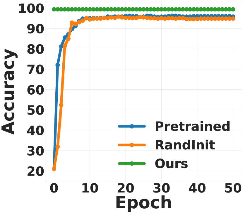
(a) Dessert Dataset

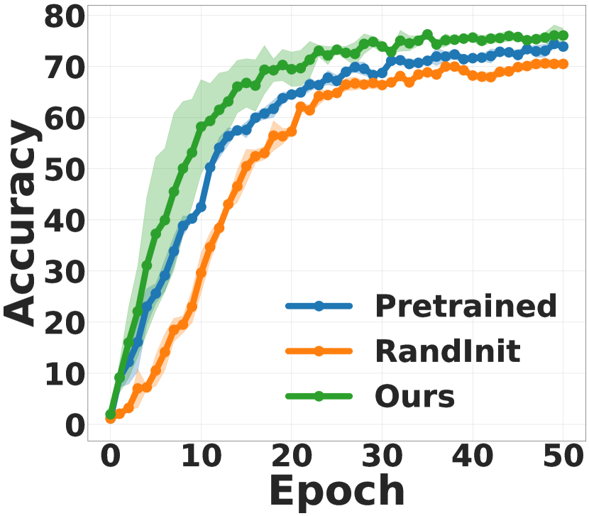
(b) Gemstones Dataset

Figure 1: We train D2NWG on a modelzoo generated from the training split of the Kaggle Dataset of  (Jeong et al., 2021) and generate weights directly for the datasets in the test split. In Figure 1(a) we sample the full set of weights using D2NWG (without any finetuning) conditioned on the dataset encoding of the Dessert dataset. For the baselines, we finetune them on the full Dessert dataset. In Figure 1(b), we again perform dataset-conditioned sampling with D2NWG and fintune it, together with a model pretrained on ImageNet and a randomly initialized model (RandInit) for 50 epochs. As can be seen, D2NWG can sample high performing weights for unseen datasets and achieves better convergence rate when the sampled weights are finetuned. The full set of results for Kaggle dataset is provided in Table 3 in the experimental section.

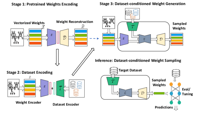
Figure 2: Stage 1: This stage consists of an encoder-decoder model trained to learn to reconstruct pretrained weights in a modelzoo. Latent embeddings from this stage are manipulated, conditioned on a dataset, in the next stages. Stage 2: In the second stage, we learn a dataset encoder for compressing a given dataset into a vector representation. The resulting dataset encoder is frozen in the next stage. Stage 3: In the third stage, we learn to manipulate the latent space of Stage 1 conditioned on the dataset encodings from Stage 2 using a diffusion model. During inference, we condition on a dataset (seen or unseen) to obtain a latent representation using the diffusion model and then decode this representation back to weights using the decoder in Stage 1. Each stage is trained independently and the blue arrow signifies joint training of Stages 1 and 2, an ablation provided in Table 8 of the Appendix.

On weight optimization automation, there exist only a handful of few related works. Schürholt et al. (2022a) proposed to learn the distribution of diverse pretrained weights enabling sampling for better initialization. Similar idea is investigated by Peebles et al. (2022), where they used prompt based fine-tuning. However, these methods do not explore the relationship of the sampled weights and target dataset. In this regard, Nava et al. (2023) proposed a meta-hypernetwork name HyperLDM class-conditioned weights generation for visual question answering(VQA) where the text descriptor of each image(classes) is used as condition.

Most existing weights generation methods for image datasets that exploit knowledge of pretrained weights are limited to unconditional parameters generation and are designed for a single model and datasets or restricted to class-conditioning such as conditioning on target loss on the same dataset. In such cases they do not take into account the correlation between the pretrained weights and the corresponding pretrained dataset. Additionally, previous works have not investigated how to properly generate weights for unseen datasets, which is a problem of significant practical importance. Therefore, we take the parameters generation problem one step further and extend it to dataset-conditioned sampling while taking advantage of existing diffusion models and pretrained weights knowledge. We propose a new method called Diffusion based Neural Network Weights Generation (D2NWG) to learn the distribution of a dataset of pretrained weights conditioned on the their corresponding dataset embeddings enabling target datasets conditioned weight generation during inference for better transfer learning as shown in Figure 1. We demonstrate generalization to seen and unseen datasets by sampling weights for an architecture conditioned on the corresponding dataset of interest. Our contributions are as follows:

• We efficiently adapt latent diffusion (Rombach et al., 2021) to network weights generation to improve the sampling performance and transfer learning.

• We combine CLIP (Radford et al., 2021) together with Set Transformer (Lee et al., 2019) for better dataset conditioning.

• Our demonstrate that our method, D2NWG, allows dataset-conditioned diverse weights sampling and can efficiently sample weights conditioned on unseen datasets.

• Through extensive experimental evaluations, we show that our method achieves promising results compared to the relevant baselines.

2 Related work

With the growing applications of neural networks, learning from pretrained weights is becoming increasingly important for speeding up the transfer learning process. Learning to generate network weights from existing modelzoos without going through the traditional training pipeline has potential to increase model efficiency. In this regard, several hypernetwork approaches have been proposed for weight prediction (Chauhan et al., 2023; Ratzlaff & Fuxin, 2020; Denil et al., 2013; Ha et al., 2016).

Deterministic Parameters Generation: Recently Zhang et al. (2019) proposed Graph Hypernetwork (GHN) for generating weights for an architecture using its directed graph representation as input. This idea was subsequently improved by Knyazev et al. (2021) in GHN2 focusing on generation across architectures for the same datasets. Analogously, Zhmoginov et al. (2022) consider weight generation as an autoregressive process and used a transformer architecture to sequentially generate weights per layer. However, this method is less scalable since it requires a transformer module per layer. Similarly, Knyazev et al. (2023) combined ideas from transformer based approach and GHN2 to improve the generalization of graph hyper networks across datasets and architectures in a new method called GHN3. Although, GHN3 achieve promising results, the sampling is deterministic, and the generalization depends solely on the generalization of the training set of architectures and pretrained dataset.

Meta Pretrained Weight Generators: Nava et al. (2023) proposed HyperLDM; a generative model for weights generation for visual question answering tasks from distribution of weights pretrained in a meta-learning setting and sampling with latent diffusion. Although generating pretrained weights through meta training is promising, the meta learning process can be computationally expensive, moreover, the meta pretrained weights are not optimal for in-distribution weights generation.

AutoEncoder-based Weight Generators: Schürholt et al. (2021) proposed to learn the distribution of weights by learning to reconstruct them using auto-encoder style architectures. A follow-up work, Schürholt et al. (2022a), proposed to learn the distribution of pretrained weights enabling unconditional sampling of diverse weights using kernel density estimation. A similar idea is developed by Peebles et al. (2022) where the weight generation is conditioned by the target loss in a diffusion transformer framework.

Diffusion Models: Denoising Diffusion Probabilistic Models (DDPM) (Ho et al., 2020; Rombach et al., 2021; Blattmann et al., 2022; Croitoru et al., 2022) enable mapping data representations to a Gaussian distribution and vice versa achieving state-of-the art performance in generative modeling. Latent diffusion models (Dhariwal & Nichol, 2021; Nichol & Dhariwal, 2021; Ho & Salimans, 2021; Zhu et al., 2023; Rombach et al., 2021) allow for manipulation of the learned latent space. We utilize such models for our dataset-conditioned weight sampling.

Our work combines components from each of the methods discussed sofar allowing for dataset-conditioned neural network weight generation for both seen and unseen datasets.

3 Approach

3.1 Preliminaries

Problem Definition: In this work, we are interested in the following problem: Given a set of neural network models of the same architecture pretrained on a set of $M$ datasets $\{\mathfrak{D}_{1},\mathfrak{D}_{2},...,\mathfrak{D}_{M}\}$, we want to learn the distribution $p(W)$ of the pretrained weights ($W$) of those models such that for a new dataset $\mathfrak{D}_{new}(x,y)$ we can conditionally sample a set of weights with $p(W_{new}|\mathfrak{D}_{new})$ that will achieve good performance on the new dataset without training or with few optimization steps.

High-Level Intuition: Our approach uses a diffusion model in order to generate a given neural architecture’s weights for previously unseen datasets. In order to train our model, we use a modelzoo of trained weights from various datasets. The diffusion model then learns from that data to predict new weights conditioned on a given dataset.

Intuitively, based on the training data, the diffusion model knows what trained networks look like and can relate this information to the characteristics of the dataset the network was trained on. At test time, for a previously unseen dataset we compute a dataset encoding and use this to guide the backward diffusion process to generate weights that mimic trained weights for this particular dataset.

This process exploits the facts that at test time we do have the dataset as input and that there is a clear relationship between a network’s trained weights and the dataset it was trained on (For a more formal argument of this relationship, please see Appendix C.) Understanding the distribution of the pretrained weights and their relation with the pretrained datasets will enable generating highly performing weights conditioned on the target dataset with or without a few optimization steps. Through the next sections we investigate the problem of learning this conditional distribution of pretrained weights.

Overview of Model: We start by describing the overall structure of our approach consisting of three main parts as shown in Figure 2. After obtaining the set of pretrained models (ie. modelzoo), we extract the pretrained weights and vectorize them into a single vector per architecture checkpoint. These vectors are then paired with their corresponding pretrained datasets. We then train a VAE model to encode the vectors to learn latent representations of weights. This stage is denoted by Stage 1 in Figure 2. In the intermediate stage we encode the dataset associated with each weight vector using a contrastive learning process denoted by the Stage 2 in Figure 2. The final stage of the proposed method, denoted by Stage 3, consists of a UNet based diffusion model. Each stage is trained separately. During inference, we encode the target dataset and use its embeddings to conditionally generate new weights for the target datasets. In the subsequent sections, we will discuss these stages in turn in detail.

3.2 Weight Encoding

Given a modelzoo of pretrained weights, we flatten the model parameters to obtain vectorized weights for each network. We then train a Variational AutoEncoder (VAE) without any conditioning. The VAE is trained such that the decoded weights, when evaluated on the test set, achieve similar performance compared to the input weights. Concretely, we minimize the following 1 objective:

$$\mathcal{L}=-\mathbb{E}_{q_{\phi}(z|x)}\left[\log p_{\theta}(x|z)\right]+\text{KL}\left[q_{\phi}(z|x)\,||\,p(z)\right]$$ (1)

where $x$ is the vectorized weight, $z$ it’s latent representation, $p_{\theta}$ and $q_{\phi}$ the reconstruction and approximate posterior terms respectively, and $p(z)$ the prior distribution. For the prior, we use the standard Gaussian with zero mean and unit variance. The trained VAE will later be used for training a latent diffusion model for dataset-conditioned weight sampling.

3.3 Dataset Encoding

To be able to sample weights conditioned on a dataset, we require an efficient mapping between the latent representations of the pretrained weights and their corresponding datasets (ie. the datasets the networks were trained on). However, efficiently encoding an entire dataset with multiple classes and hundreds, even millions, of samples per class is a challenging task. One way to encode such datasets is to utilize dataset condensation techniques which consists of training a network to synthesize one example per classes, combining the class-wise condensations and using it as a representation for the dataset. However this process requires performing the same process for every test dataset increasing the computation cost of the model. Hence we explore existing dataset-adaptive Neural Architecture Search approaches Jeong et al. (2021); Lee et al. (2021) where Set Transformer (Lee et al., 2019) has been demonstrated as an efficient model for dataset encoding.

Set-based Dataset Encoding: Given a dataset $\mathfrak{D}=\{x_{i},y_{i}\}_{i=1}^{N}$, where $x_{i}$ and $y_{i}$ are input-output pairs, we form subsets $s_{i}=(x_{p}^{y_{i}})_{p=1}^{K_{i}}$ with $K_{i}=|s_{i}|$, and ${s_{i}}\in\mathbb{R}^{K_{i}\times d}$. If $\mathfrak{D}$ is an image dataset, $d=c\times h\times w$ where $c$, $h$ and $w$ correspond to the image channel, height and width respectively. Therefore, the entire dataset can be viewed as a collection of subsets $\mathcal{S}=\{s_{i}\}_{i=1}^{C}$ with $C$ being the number of distinct classes. To encode such dataset, we define a transformation $\mathcal{T}$ over the subsets that takes each set $s_{i}$ and outputs an embedding $z_{s_{i}}\in\mathbb{R}^{1\times d}$. We note the abuse of notation here where $z$ has been used for the weight embedding in Section 3.2. All embeddings are aggregated to form a new embedding set $\tilde{s}_{i}\in\mathbb{R}^{C\times d}$ to which we apply another transformation $\mathcal{T}$ to $\tilde{s}_{i}$ to the encoded dataset to $z_{\mathfrak{D}}\in\mathbb{R}^{d}$. The encoding mechanism described above can be summarized as a composition of Set Transformer blocks $\mathcal{T}$ as follows $z_{\mathfrak{D}}=\mathcal{T}o\mathcal{T}(\mathcal{S})$. To recapitulate, we refer to this operation of encoding the dataset as $\mathcal{T}$. Training the Set Transformer modules together with the different modules in the pipeline can be computationally demanding. To resolve this issue, we next outline a CLIP style objective for training the Set Transformer Modules.

Contrastive Dataset Encoding: To improve the effectiveness of the dataset encoding mechanism on large collections of datasets, we train the Set Transformer using a CLIP-style contrastive loss. An analogous idea is exploited in HyperCLIP (Nava et al., 2023). However in our case, we replace the image encoder with the VAE of Section 3.2, and replace the image-text contrastive pairs with the weight embedding and its corresponding dataset embedding. Concretely, we utilize the following contrastive pair, $\text{Embed}((\mathfrak{D}_{i}(x_{j},y_{j})_{j}^{c_{i}},W_{i}))=(z_{\mathfrak{D}_{i}},z_{i})$ consisting of the class-wise dataset encodings and the VAE embedding of a corresponding network weight. Using the pretrained VAE encoder of Section 3.2, we train the Set Transformer dataset encoding module $\mathcal{T}$ to align its embedding $z_{\mathfrak{D}_{i}}=\mathcal{T}(\mathfrak{D}_{i}(x_{j},y_{j})_{j}^{c_{i}})$ where $z_{\mathfrak{D}_{i}}\in\mathbb{R}^{1\times d_{z}}$ with the network embeddings $z_{i}$ of the pretrained VAE. The Set Transformer training objective is given as:

$$\mathcal{L}_{CLIP}=-log\frac{exp(z_{i}.z_{\mathfrak{D}_{i}/\tau)}}{\sum_{k=0}^{N}exp(z_{i}.z_{\mathfrak{D}_{k}}/\tau)}$$ (2)

3.4 Dataset-Conditioned Weight Generation

At this stage, we have access to a pretrained VAE for encoding neural network weights and a pretrained Set Transformer module for encoding entire datasets. The next stage involves defining a model to generate latent representations of weights conditioned on dataset representations. We achieve this by using Diffusion Denoising Probabilistic Models (DDPM) (Ho et al., 2020; Rombach et al., 2021).

Forward Process: Given a weight embedding $z$, obtained from the encoder of the pretrained VAE, the forward diffusion process involves successive Gaussion noise perturbations of $z$ over $T$ time steps. At time step $t$,

$$p(z_{t}|z_{t-1})=\mathcal{N}(z_{t};\mu_{t}=\sqrt{1-\beta_{t}}z_{t-1},\beta_{t}I)$$ (3)

where $\beta_{t}\in(0,1)$ is the noise variance and $p(z_{1:T}|z_{0})=\prod_{i=1}^{T}p(z_{t}|z_{t-1})$.

Reverse Process: As in most DDPM approaches the reverse process is approximated by a neural network such that:

$$p_{\theta}(z_{t-1}|z_{t})=\mathcal{N}(z_{t-1};\mu_{\theta}(z_{t},t),\Sigma_{\theta}(z_{t},t)),$$ (4)

where $\mu_{\theta}$ and $\Sigma_{\theta}$ are neural networks.

Dataset-Conditioned Training: The diffusion model is trained on the VAE embeddings $z$, conditioned on the dataset encodings through concatenation. To take advantage of existing architectures, we design the VAE model to produce latent representations compatible with existing latent diffusion models with minimal modifications and optimize the following latent diffusion model objective:

$$\mathcal{L}_{LDM}=\mathbb{E}_{z,\varepsilon\sim\mathcal{N}(0,1),Z_{\mathfrak{D}},t}\left[||\varepsilon-\varepsilon_{\psi}(z_{t},z_{\mathfrak{D}},t)||^{2}_{2}\right],$$ (5)

where $\varepsilon_{\psi}(z_{t},z_{\mathfrak{D}},t)$ is implemented as a UNet.

Sampling: New weights are sampled conditionally through the revers diffusion process as follows:

$$z_{t}=\frac{1}{\sqrt{a_{t}}}(z_{t}-\frac{\beta_{t}}{\sqrt{1-\tilde{a}_{t}}}\varepsilon_{\psi}(z_{t},z_{\mathfrak{D}},t,))+\sigma\xi,$$ (6)

where $\xi\sim\mathcal{N}(0,I)$ and, $\sigma_{t}$ a chosen value. After sampling a latent representation $\bar{(}z$ for a given dataset $\mathfrak{D}_{i})$. The pretrained VAE decoder is used to transform that latents into a weight $\bar{w}=\mathcal{D}(\bar{z})$ which is then used to initialize the target network as depicted in Figure 2.

4 Experiments

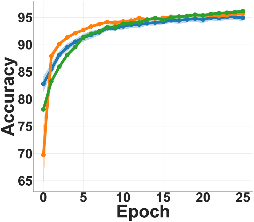
(a) MNIST

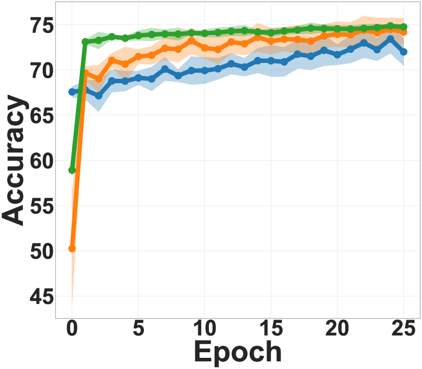
(b) SVHN

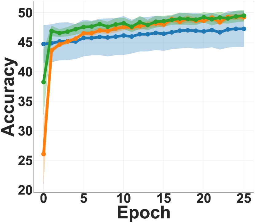
(c) CIFAR-10

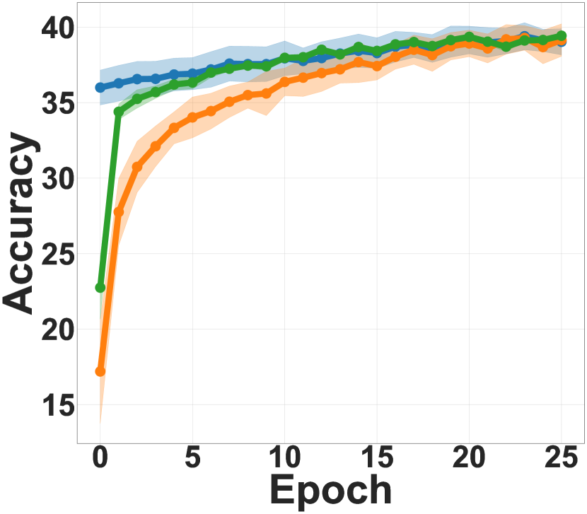
(d) STL-10

Figure 3: Convergence Plots on Fintuning Generated Weigths: Weights generated by the competing methods are finetuned for 25 epochs on the training set. We utilize the modelzoos of  Schürholt et al. (2022b).

We generate and evaluate weights in the following setting:

• Weight Generation without Finetuning: For this task, we condition on a dataset, generate weights and directly evaluate it on the test set.

• Weight Generation with Finetuning: The generated weights are finetuned on the training set for a fixed number of epochs before evaluating on the test set.

Baselines: We benchmark against the following:

• RandInit: This is a randomly initialized model trained on the training set of the target dataset from scratch for a specified number of epochs.

• Pretrained: These are models pretrained either on the target dataset or ImageNet. We follow the setting of Schürholt et al. (2022a) and train this baseline for 25 epochs on the target datasets in Tables 3 & 2. All other pretranied baselines are trained on ImageNet.

• S_KDE30 (Schürholt et al., 2022a): This method learns an autoencoder on a modelzoo of networks trained on a single dataset and uses Kernel Density Estimation (KDE) to sample new weights from the embedding of networks in the modelzoo.

Detailed experimental setup is outlined in the Appendix.

Modelzoo Generation: We utilize the pretrained weights datasets of Schürholt et al. (2022b) which consists of four modelzoos of networks pretranied on MNIST, SVHN, CIFAR-10 and STL-10. Next we generate a modelzoo for the set of datasets introduced in Jeong et al. (2021) and refer to it as the KaggleZoo. The test datasets are used for weight generation on unseen tasks. Finally, we generate a modelzoo by creating 2000 subsets of ImageNet with 100 and 50 images per class in the training and test splits respectively. Additionally, we do not train on the CIFAR-10 and STL-10 modelzoos of Schürholt et al. (2022b) and use them for unseen dataset weight generation. Details for generating the modelzoos is provided in Appendix B.

Algorithm 1 Datasets Encoder Training

  Input: pretrained weights $x$, image features $y$, batch_num $m$

  Instanciate $\mathcal{T}={\verb|Set Transformer|}$, Load pretrained Encoder ($\mathcal{E}$).

  repeat

     Initialize $loss=0.0$

     for $i=1$ to $m-1$ do

        $x_{i}\sim x$, $\mathfrak{D_{i}}\sim\mathfrak{D}$

        $z_{i}=\text{Encoder}_{\text{VAE}}(x_{i})$

        $z_{\mathfrak{D}_{i}}=\mathcal{T}(\mathfrak{D_{i}})$

        $loss=loss+\mathcal{L}_{CLIP}(z_{i},z_{\mathfrak{D_{i}}})$ (Equation 2)

     end for

     Update weights of $\mathcal{T}$

  until convergence

Set-based Dataset Encoding: We use Set Transformer (Lee et al., 2019) for dataset encoding using features extracted from CLIP (Radford et al., 2021) similar to the approach in Lee et al. (2021) where features were extracted using a pretrained ResNet18. This process is done before training with the dataset encoder defined in Section 3.3. We observed that jointly optimizing the dataset encoder with the diffusion model is more challenging given a large number of datasets hence we pretrain the dataset encoder and freeze it during the training of the diffusion model.

Compute: For the zoo generation we use a single Titan RTX GPU with 24GB memory. The proposed model was also trained on a single GPU with 24GB memory.

4.1 In-distribution Transfer Learning

Task: The main objective of this experiment is to evaluate convergence speed using weights from each of the methods as initialization. In this experiment the target dataset is the same as those used to generate the modelzoos.

Setup: The pretrained weights used here are from epochs 21 to 25 for each dataset where 70% of the resulting modelzoo is used for training and 15% for validation and testing respectively. The number of pretrained weights in the modelzoos are 3500 for MNIST, CIFAR-10, and STL-10, and 2864 for SVHN. The flattened network weights’ length is 2864 for CIFAR-10 and STL-10 and, 2464 for MNIST and SVHN. We pad all the weights with zero to 2864. After training the diffusion model, we conditionally sample five set of weights based on images samples from the corresponding datasets and initialize each corresponding architectures and then finetune them for 25 epochs. We compare our method to the best approach in Schürholt et al. (2022a) and the pretrained weights already trained for 25 epochs (we evolve this model for 25 more epochs resulting in 50 epochs of optimization on the training set).

Table 1: Convergence Speed Comparison Sampled weights from S_KDE30 (Schürholt et al., 2022a) and our method are evaluated on the test set after 0 (meaning no optimization steps), 1 and 25 epochs of training on the training set. The Pretrained baseline is trained on the training set for a total of 50 epochs.

Model	Epoch	MNIST	SVHN	CIFAR-10	STL-10
Pretrained	50	95.70	74.49	49.25	39.39
SKDE30	0	69.73	50.25	26.06	17.20
D2NWG (Ours)	0	78.10	58.92	38.23	22.74
SKDE30	1	82.69	70.45	44.75	28.42
D2NWG (Ours)	1	83.25	73.11	46.88	34.39
SKDE30	25	95.70	74.69	49.14	39.14
D2NWG (Ours)	25	96.17	74.75	49.48	39.43

Results: As reported in Table 1, D2NWG consistently speeds up the convergence rate on the related tasks and after 25 epochs, achieves better performance than the pretrained model, consistently outperforming the Kernel Density Estimation approach of  Schürholt et al. (2022a). In Figure 3, we show the convergence plots for the 4 datasets considered in this task.

Table 2: No Fine-tuning Initialization on Unseen Datasets We transfer from one dataset, or combinations of datasets, to unseen datasets at test time.

Source	Target	Accuracy	Methods
MNIST	SVHN	13.25	SKDE30
SVHN	MNIST	29.30
CIFAR-10	STL-10	15.20
STL-10	CIFAR-10	15.40
Sampling from Combined Weights Distribution
MNIST+CIFAR-10	SVHN	18.80	Ours
MNist+CIFAR-10	STL-10	16.21
SVHN + STL-10	MNIST	36.64
SVHN + STL-10	CIFAR-10	18.00

4.2 Sampling Weights for Unseen Datasets

Task: We evaluate the transferability of the models on unseen datasets. We create disjoint modelzoos by combining MNIST and CIFAR-10 into a single modelzoo and combining the SVHN and STL-10 modelzoos. When we train on the MNIST plus CIFAR-10 modelzoos, we test on the SVHN and STL-10 modelzoos and vice-versa.

Results: As shown in Table 2, the D2NWG is able to sample weights with higher accuracy on unseen datasets as well as for in distribution. Through these experiments our method does not only outperform the baseline it also demonstrates promising results for dataset-conditioned sampling for unseen datasets.

4.3 Performance Evaluation on KaggleZoo

We extend the performance evaluation on unseen dataset to much diverse datasets. Since the baseline Schürholt et al. (2022a) relies on unconditional sampling this method is not appropriate for unseen dataset evaluation. Therefore the baseline of this experiments are model pretrained on ImageNet and random initialization.

Task: In this experiment, we aim to demonstrate that D2NWG can generate efficient weights for initialization and fine-tuning compared to random initialization and ImageNet pretrained models on unseen datasets with different number of classes than those encountered during training.

Table 3: Dataset Conditioned Sampling Weight sampling on 10 unseen real-world datasets. We report two sets of results: (a) weight evaluation without finetuning and (b) weight evaluation after 50 epochs of finetuning. The pretrained baseline is trained on ImageNet1K. We report the accuracy on the testset.

Datasets	Initialization			Fine-tuning
	RandInit	Pretrained	D2NWG	RandInit	Pretrained	D2NWG
Gemstones	1.13	0.62	1.86	70.59	67.49	76.06
Dog Breeds	0.55	0.69	1.87	80.78	78.13	80.88
Dessert	21.03	12.50	99.40	95.83	94.64	99.40
Colorectal Histology	11.77	11.00	18.12	90.34	89.75	93.65
Drawing	10.86	11.00	11.87	90.20	90.00	89.00
Alien vs Predator	51.48	28.88	78.15	98.52	98.89	97.77
COVID-19	20.13	46.53	47.22	93.86	93.40	94.56
honey-bee-pollen	49.54	50.00	56.94	93.05	88.89	93.55
Speed Limit Signs	30.55	25.00	31.48	83.33	86.11	90.74
Japanese Characters	0.03	0.08	0.50	53.17	62.33	62.16

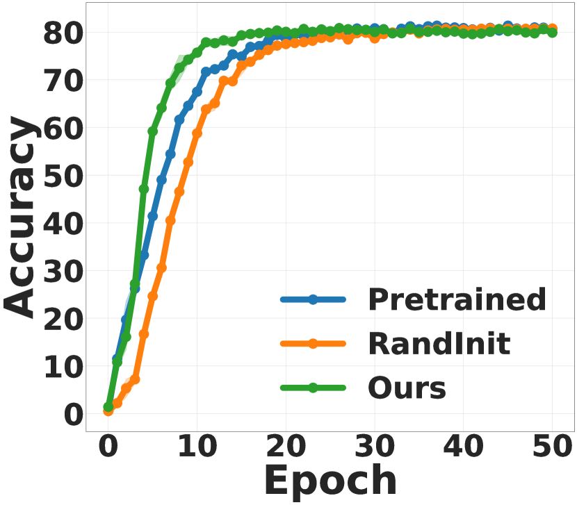
(a) Dog Breeds

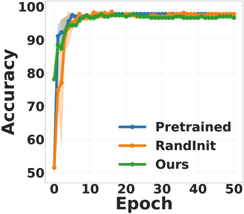
(b) Alien vs Predator

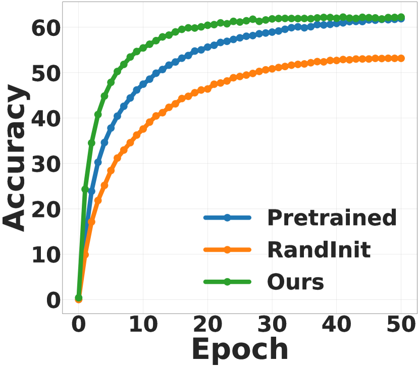
(c) Japanese Characters

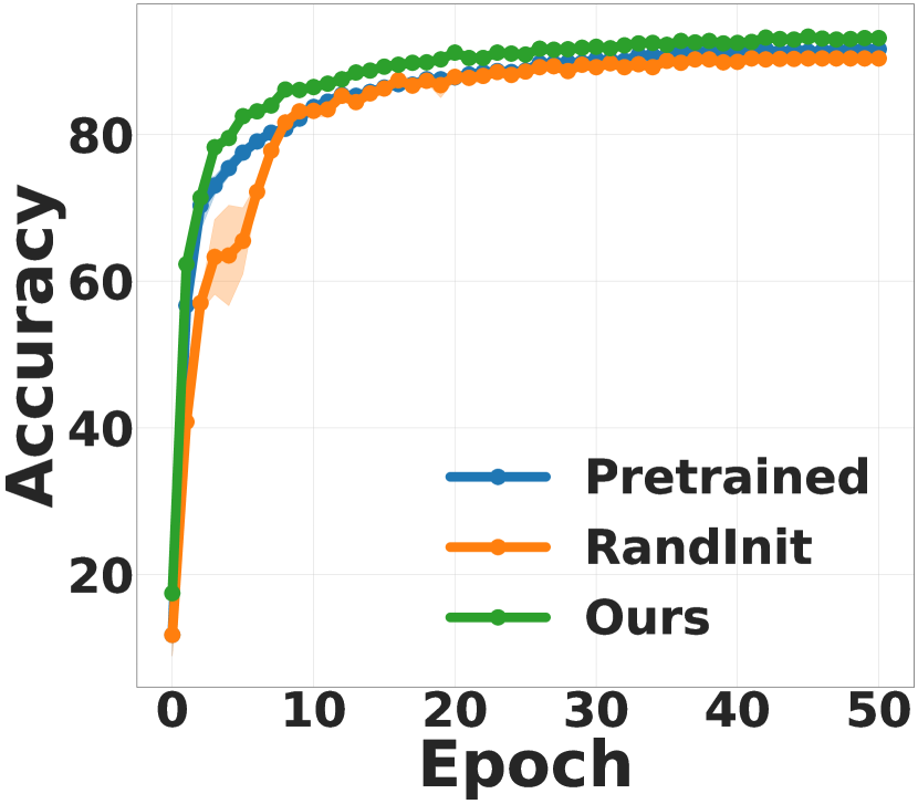
(d) Colorectal Histology

Figure 4: Average accuracy evolution of fine-tuning for 50 epochs with sampled weights for unseen datasets from real world datasets The full results are reported in the appendix

Results: As show in Table 3 and in the convergence plots in Figure 4, weight initialization with D2NWG without any fine-tuning achieves 99.04% on dessert dataset outperforming the random initialized model trained for 50 epochs. Additionally, our method consistently speeds-up the convergence on all tasks compared to the random initialized and pretrained models. Except on Japanese Characters, Gemstones and Dog Breeds datasets where both methods achieved similar results, the proposed method consistently outperformed the two baselines and converges faster on the finetuning task. Although the test subsets and the training subsets of image dataset have no overlapping classes our method is able to transfer well to the test set.

We investigate the reason why the proposed method achieves superior performance on some datasets. Our findings suggest that D2NWG achieves similar none finetuning performance as the random initialization in the cases where the target dataset has more classes than the maximum number classes in the pretrained datasets. The sapmled weight performance on the dessert dataset is due to the fact that this dataset contains similar images as those in the foods dataset which are a subsets of the food classification task in the pretrained image datasets. These results showed that the dataset encoder efficiently encodes the datasets and if some target datasets overlap with those in the modelzoo, the proposed method is able to retrieve the weights that transfer well. Detailed results can be found in Appendix H.

Table 4: Cross-Dataset Trasfer MNIST$\rightarrow$ SVHN, SVHN$\rightarrow$ MNIST, CIFAR-10$\rightarrow$ STL-10, STL-10 $\rightarrow$ CIFAR-10. The OFA model is pretrained on ImageNet.

Model	MNIST	SVHN	CIFAR10	STL10
Pretrained (seen)	97.44	84.04	81.83	66.62
D2NWG (seen)	97.49	83.12	82.19	66.13
OFA (Pretrained)(Cai et al., 2020)	13.34	8.90	13.34	8.90
cross_dataset (unseen)	50.70	28.68	34.16	39.95
D2NWG (unseen)	49.32	29.13	35.02	39.90
D2NWG+average (unseen)	50.24	29.13	35.03	40.00

Evaluation on Larger Architectures: So far we have restricted ourselves to modelzoos populated by realitively simple CNN architectures. In this section we evaluate our method on MobileNetV3, a subnetwork sample from OFA (Cai et al., 2020) pretrained on CIFAR-10, STL-10, SVHN and MNIST for 25 epochs. The last 10 checkpoints per dataset are collected and we learn the pretrained weights distribution using our method. The performance of the sampled weighs are presented in Table 4 and shows that the proposed method transfers well to unseen dataset as well as on seen datasets. In the last row of Table 4, we provide ModelSoup-type (Wortsman et al., 2022) experiments where we average multiple weights sampled from our model.

4.4 Ablation study

In this section, we investigate the importance and limitation of the different modules used to build our method.

4.4.1 Effect of Modelzoo Size Generalization

In this part we investigate whether increasing the number of datasets will increase the performance on unseen datasets. To achieve that goal, we perform experiments with modelzoos of size 5000, 10000 and 20000 created from subsets of ImageNet. We use CIFAR-10 and STL-10 as unseen target datasets. We sample 50 weights and report the average of the top 5 performing weights in Figure 5(a) where it can be observed that increasing the modelzoo size improve generalization.

Results: On CIFAR-10 and STL-10, we obtain accuracies of 39.60$\pm$1.31% and 44.66 $\pm$ 0.55% for 5000 subsets, 42.15$\pm$2.12 and 64.83 $\pm$ 2.83 for 10000 subsets, and 52.64$\pm$3.12% and, 80.49 $\pm$ 1.77% for 20000 subsets. The maximum accuracy with random initialization are 12.11%, and 17.12% on CIFAR-10 and STL-10 with no fine-tuning.

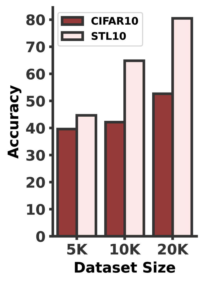
(a)

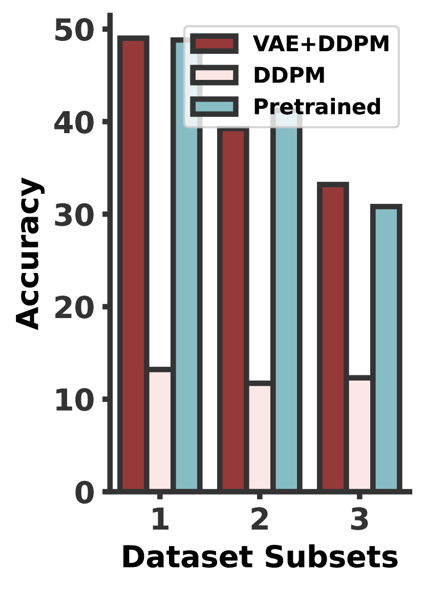
(b)

Figure 5: (a) Effect of the number of pretrained datasets on sampling weights performance on unseen datasets. (b) Performance comparison on in-distribution sampling of methods with VAE+DDPM vs DDPM

4.4.2 Sampling without Latent Representation

We investigate a variant of our model that learns the diffusion model directly on the weights without the AutoEncoder stage. We compare these two setting, with and without the AutoEncoder. Both variants are trained on 1000 subsets of ImageNet. We report the results of in-distribution sampling on three datasets in Figure 5(b).

Results: As reported in Figure 5(b), for the same diffusion architecture, it is much easier to learn the pretrained weights distribution in latent space. One of the reason for which the DDPM process failed on the raw pretrained may be due to the fact that raw pretrained weights may require higher model capacity. Note also that learning the diffusion model directly on the weight space is computationally expensive. Hence, perhaps learning diffusion on subsets of the weights might be a more promising direction both in terms of computation and performance and we leave this as future work.

4.4.3 CLIP-based Dataset Encoding

We further investigate the different between CLIP-based dataset encoding scheme trained in an intermediate stage and the Set Transformer encoder jointly trained with the diffusion process. We conduct the experiments on the 140 Kaggle datasets and their corresponding modelzoos.

Results: We compare the in-distribution sampling, out-distribution initialization, and fine-tuning results. As shown in Figure 6, for in-distribution sampling both methods achieve similar results for small number of datasets. When the number of datasets increases the set-transformer jointly trained with diffusion approach struggle to converge.

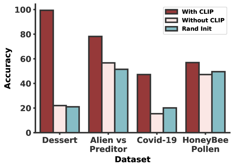
Figure 6: Performance comparison at initialization of method with jointly trained set-transformer (Without CLIP) and method clip-based dataset encoder.

5 Conclusion

In this work we presented a three stage approach to neural network weight generation that involves fitting an AutoEncoder to pretrained weights, learning a dataset encoder using CLIP embeddings and learning a diffusion model to manipulate the latent space conditioned on the dataset embeddings. We demonstrated that the proposed method can sample high quality weights for both seen and unseen datasets and achieves better performance when finetuned for a fixed number of epochs when benchmarked against the relevant baselines.

Appendix A Discussion

Broader Impact D2NWG addresses the resource-intensive nature of deep learning by proposing a method for efficient transfer learning. This has the potential to reduce the computational resources required for training neural networks, making it more accessible to a wider range of researchers and organizations.

Limitation In this work we focus mainly on generalization across datasets. Therefore, sampling for unseen architecture may not guarantee performance improvement. Additionally, while diffusion model may achieve impressive performance on image generation, there are still some challenges to efficiently recast it for weights generation including memory constraint and convergence challenge.

Appendix B Details of Modelzoo Generation

The code source will be released on Github https://github.com/sorobedio/DNNWG

B.1 Modelzoo and Pretrained Datasets

All MLP based modelzoos are trained with Adam optimizer with learning rate 1e-3 for 30 epochs. And we collect the checkpoints from epochs 20 to 30.

Model zoo We use the pretrained datasets from Schürholt et al. (2022b) as structured in (Schürholt et al., 2022a). This dataset consists of 4 different datasets with 5000 pretrained weights per architectures and datasets. The details of the architecture used to generate the pretrained weights are available in Schürholt et al. (2022b).

KaggleZoo The datasets used to generate this modelzoo generation is the same as those defined in (Jeong et al., 2021). To efficiently generate the pretrained weights, we first compute the features of each image then use a MLP with two layers with input size 512 hidden size 256 with leaky_relu activation. We train the MLP on clip features because it allows us to quickly generate high performing weights. For each datasets we used the last 10 checkpoints which results in 1400 pretrained vector for training.

ImageNet zoo To generate the pretrained modelzoo on ImageNet, we sample respectively 1000, 5000, 10000 and 20000 subsets with 10 classes respectively and 100 images per class in the training set and 50 for per class in test set. For 1000 and 5000 subsets we used the same MLP architecture as the KaggleZoo. For the 10000 we reduce the hidden dimension to 128 and, for 20000 subsets we only use one linear probing layer. On the other datasets linear probing shows similar generalization performance similar to the two layer MLP architectures. Reducing the model size is motivated by the computation cost. We use Adam optimizer with learning rate set 1e-3. All models are trained for 30 epochs.

Appendix C Relationship Between Datasets and Trained Weights

Nowadays, gradient descent based optimization is the commonly used technique to generate optimal neural network weights through training by minimizing a loss function, ie. cross-entropy for classifiation tasks. The weights optimized with gradient descent thus contains some information about the training data. Therefore, understanding the correlation between the training dataset and the optimal weights is important for the generation of weights.

During the optimization process with gradient descent the weights of each layer $i$ are updated as $w_{i}=w_{i-1}-\eta\nabla_{w_{i}}\mathcal{L}(w_{1},w_{2},\ldots,w_{n})$, where $\nabla_{w_{i}}\mathcal{L}(w_{1},w_{2},\ldots,w_{n})$ is input dependent. As an example, let’s consider a two-layer neural network with feedforward operations as follows;

$$x :inputs$$

$$l_{1} =W_{1}x+b_{1} h =ReLU(l_{1})$$

$$h =ReLU(l_{1}) l_{2} =W_{2}h+b_{2}$$

$$\hat{y} =softmax(l_{2}) J =CE(y,\hat{y})$$

Analysing the weights’ update below, we can observe that the optimal weights are noisy perturbation of the inputs features map and all together they contain information about the training either related to the raw input or the feature map at a given stage.

$$\delta_{1} =\frac{\partial J}{\partial l_{2}}=(y-\hat{y})^{T}$$

$$\delta_{2} =\frac{\partial J}{\partial l_{1}}=\delta_{1}W_{2}osgn(h)$$

$$W^{(i+1)}_{1} =W^{(i)}_{1}-\eta\nabla_{w_{1}}\mathcal{L}(w_{1},w_{2},b_{1},b_{2})$$

$$=W^{(i)}_{1}-\eta\delta_{2}^{T}x$$

$$W^{(i+1)}_{2} =W^{(i)}_{2}-\eta\nabla_{w_{2}}\mathcal{L}(w_{1},w_{2},b_{1},b_{2})$$

$$=W^{(i)}_{2}-\eta\delta_{1}^{T}h^{T}$$

Appendix D Predictor Training

To improve the reconstruction and sampling efficiency, we trained an accuracy predictor $g$ from pretrained weights $w$ then use the frozen predictor during the the training of the VAE as L₂-regularizer as defined in Equation 7.

$$\underset{\theta,\sigma}{\min}\frac{w-f_{\theta}(w)}{\sigma^{2}}+\log\sigma^{2}+||g(w)-g(f_{\theta}(w))||^{2},$$ (7)

where $g(w)$ is the embedding of the original input and $g(f_{\theta}(w))$ is the predictor embedding of the reconstructed weights. The predictor can be either dataset-conditioned or unconditioned. In general we found that dataset-conditioned predictor works only well for large number of samples per dataset. After the AutoEncoder is trained, we train the dataset-conditioned module which requires a dataset encoder.

Algorithm 2 predictor-guided VAE

  Input: pretrained weights $x$, accuracy $y$, batch_num $m$

  Instanciate $\mathcal{f}=set\_transformer$, Load pretrained predictor ($\mathcal{g}$).

  repeat

     Initialize $loss=0.0$

     for $i=1$ to $m-1$ do

        $\bar{x}=f_{\theta}(x)$, $\bar{y}=g(\bar{x})$ $\hat{y}=g(x)$

        $\underset{\theta}{L}\frac{x-\bar{x}}{\sigma^{2}}+\log\sigma^{2}+||\hat{y}-\bar{y}||^{2}$

     end for

     Update weights of $\mathcal{f}$

  until convergence

Appendix E Details of the Proposed Model

We build our dataset conditioned weight generation model using latent diffusion (Rombach et al., 2021).

AutoEncoder: We use the same VAE modules of latent diffusion with minor modifications and use the same structure for all experiments except adaptation of the inputs and output dimensions. We insert a linear layer before the first layer of the encoder such that we can reshape its output to a representation for the convolution layers. Analogously, another linear layer is place as the last layer of the decoder adapting the output to the vectorized weights representations. For the VAE loss function we removed the discriminator in the original latent diffusion VAE.

Diffusion Model: Regarding the diffusion process, we use an architecture similar to the UNet model as in latent diffusion with minor changes. The training process in this module is the same as in latent diffusion.

Dataset Encoder: We investigated three different mechanisms of dataset encoding. Firstly, we use Set Transformer which can be difficult to train when optimized together with the diffusion using the weights encoder from the VAE and the Set Transformer. Finally, we also observe that two linear layers can also be used to efficiently mimic the Set Transfomer. The main limitation of the contrastive based dataset encoding with Set Transformer is that this method can easily overfit the training datasets while jointly optimizing Set Transformer with the diffusion process often takes longer to converge.

Alternate Dataset Encoding Mechanisms We also use a two-layers MLP model as dataset encoder. The first layer is a dynamic layer with a maximum input feature size set to $n\_max.c\_max$ with $n\_max$ max number of images per class and $c\_max$ maximum number of classes among all subsets of pretrained datasets. The shape of the each images datasets features obtained with clip image encoder is $x\in\mathbf{R}^{c\times n\times d}$ with $d$ the features dimension for each corresponding pretrained weight vector. While the Set Transformer based encoder uses these inputs directly, with MLP encoder we reshape each input $x\in\mathbf{R}^{c\times n\times d}\rightarrow x\in\mathbf{R}^{d\times nd}$ then applied the dynamic linear layer.If a dataset has more classes respectively more samples than $c\_max$ respectively $n\_max$, we only consider the first $c\_max$ classes and $n\_max$ samples per classes. In the case that the dataset has less classes or samples we reset the dynamic linear layer dimension accordingly. The output of the dynamic linear layer is $z\in\mathbf{R}^{d\times h}$ where $h$ s an arbitrary chosen number $h>0$. We then reshape $z\in\mathbf{R}^{d\times h}$ to $z\in\mathbf{R}^{1\times hd}$ ($hd$ fixed) and apply the final linear layer to obtain the desired output. This model can be jointly optimized with diffusion model while achieving good performance.

Pretrained Set Transformer We make use of Set Transformer for dataset encoding pretrained in (Lee et al., 2021). The idea is to use the frozen Set Transformer then add a single linear layer to adapt the output to our problem and use it as dataset encoder. This approach reduces the computation cost of training the Set Transformer enabling jointly optimization of the dataset encoder and the diffusion model. We provide the results of these datasets encoding schemes in Table8 on the Hyperzoo dataset.

Table 5: Models seting, $n$ and $c$ in the dataset configuration represent respectively the number of samples per class n=5 for training and c the total number of classes per dataset. The VAE and the diffusion models share similar configuration and architectures as (Rombach et al., 2021)

Parameters	Values
epochs	[50, 2000]
VAE model
optimizer	Adam
Learning rate	1e-3
latent_size	1024
kl_weights	1e-6
Dataset encoder
architecture	Set transformer
input dim	$c\times n\times 512$(min)
output dim	1024 (min)
number of set transformers	2
Diffusion
optimizer	AdamW
base learning rate	1e-4
scheduler	linear
Time step	1024
backward network	Unet
input to Unet	$(c\times 32\times 32)$

Appendix F Training Details

Training D2NWG. The training process consists of two main stages: In stage 1 we train the predictor then unconditionally train the VAE accoding to equation 7. However, we also train the VAE following equation 1 without a predictor in the main experiments. In stage 2 we train the LDM module with the Set Transforter based dataset encoding module(not that depending on the choice of dataset encoder, another pretraining stage may be required). Although, the dataset encoder can be optimized together with the diffusion processes, we prefer to train them separately to speed-up the training process while reducing the memory requirement. The VAE and the dataset encoder are trained with Adam optimizer and learning rate set to 1e-4. The diffusion model in each experiment is trained with a linear scheduler, base learning rate 1e-4 and, AdamW optimizer as defined in (Rombach et al., 2021). During the training process of the diffusion model the output of the dataset encoder is concatenated to the latent representation of the input weights forming the input to the UNET module. Additionally, we investigate joint training of the diffusion process in the ablation study and appendix section 4.4.3 E. Additional details can be found in Table 5

Appendix G Additional results

G.1 Fast Convergence Performance Evaluation

In this section we report supplementary results for experiment in section 4.1 in Table 6 which is a full version of Table 1.

Table 6: Convergence speed comparison with S_KDE30 (Schürholt et al., 2022a).

Model	Epoch	MNIST	SVHN	CIFAR-10	STL-10
Pretrained models	25	82.82$\pm$ 1.38	67.57$\pm$ 0.59	44.68$\pm$ 3.15	35.99$\pm$ 1.15
SKDE30	0	69.73$\pm$ 5.12	50.25$\pm$ 6.12	26.06$\pm$ 3.01	17.20$\pm$ 3.43
D2NWG (Ours)	0	78.10$\pm$0.29	58.92$\pm$ 0.76	38.23$\pm$ 5.45	22.74$\pm$ 2.08
Pretrained models	26	85.50$\pm$ 0.99	67.79$\pm$ 1.05	44.81$\pm$ 3.20	36.28$\pm$ 1.18
SKDE30	1	82.69$\pm$ 0.81	70.45$\pm$ 0.92	44.75$\pm$ 0.81	28.42$\pm$ 1.53
D2NWG (Ours)	1	83.25$\pm$ 0.25	73.11$\pm$0.24	46.88$\pm$ 0.85	34.39$\pm$ 0.51
Pretrained models	50	95.70$\pm$ 0.36	74.49$\pm$ 1.53	49.25$\pm$ 3.00	39.39$\pm$0.89
SKDE30	25	95.70$\pm$ 0.30	74.69$\pm$ 0.70	49.14$\pm$ 0.65	39.14$\pm$ 0.76
D2NWG (Ours)	25	96.17$\pm$0.0.33	74.75$\pm$ 0.33	49.48$\pm$ 0.97	39.43$\pm$ 0.13

Appendix H Detail of Experimental Results

H.1 Coupling with Accuracy Predictor

This section reports the extended results of Table 2 in which we compared our method in-distribution and out-of distribution with and without accuracy predictor.

Results.: The full results of Table 2 are reported in Table 7. Using an accuracy predictor enable easily selecting highly performing when sampling in-distribution. However, in our case the accuracy predictor struggles to generalize well for unseen dataset as shown in Table 7

Table 7: Performance evaluation at initialization without fine-tuning. For the baseline we use weights of SVHN for MNIST and vice versa similarly for CIFAR-10 and STL-10

Datasets	MNIST	SVHN	CIFAR10	STL10
Random	10.23$\pm$0.56	12.21$\pm$3.76	9.98$\pm$1.47	9.56$\pm$1.02
Pretrained models	82.82$\pm$ 1.38	67.57$\pm$ 0.59	44.68$\pm$ 3.15	35.99$\pm$ 1.15
Skde30Schürholt et al. (2022a)	69.73$\pm$ 5.12	50.25$\pm$ 6.12	26.06$\pm$ 3.01	17.20$\pm$ 3.43
seen (D2NWG)	83.92$\pm$1.92	61.81 $\pm$ 3.13	43.08$\pm$0.55	31.45$\pm$0.35
seen(D2NWG)(with Pred)	84.85$\pm$0.83	66.03 $\pm$ 1.36	43.89$\pm$0.15	34.29$\pm$0.13
Skde30Schürholt et al. (2022a)(cross)	29.30$\pm$ 3.46	13.25$\pm$ 1.12	15.40$\pm$ 0.51	15.20$\pm$1.24
not seen(D2NWG)	36.64$\pm$4.69	18.80$\pm$0.58	18.00$\pm$0.22	16.21$\pm$0.52
not seen(D2NWG)(with Pred)	30.15$\pm$5.09	15.76$\pm$1.43	17.10$\pm$1.12	15.37$\pm$0.52

Table 8: In-distribution performance comparison of different image dataset encoding schemes on model zoo dataset

Datasets	MNIST	SVHN	CIFAR10	STL10
Pretrained models	82.82$\pm$ 1.38	67.57$\pm$ 0.59	44.68$\pm$ 3.15	35.99$\pm$ 1.15
Skde30Schürholt et al. (2022a)	69.73$\pm$ 5.12	50.25$\pm$ 6.12	26.06$\pm$ 3.01	17.20$\pm$ 3.43
MLP_Encoder	67.04$\pm$17.73	35.65 $\pm$ 13.03	17.41$\pm$3.02	20.36$\pm$7.38
Set_transf(pret)	78.21$\pm$1.76	60.90 $\pm$ 1.08	28.68$\pm$1.84	34.75$\pm$00.38
seen (D2NWG)	83.92$\pm$1.92	61.81 $\pm$ 3.13	43.08$\pm$0.55	31.45$\pm$0.35
seen(D2NWG)(with Pred)	84.85$\pm$0.83	66.03 $\pm$ 1.36	43.89$\pm$0.15	34.29$\pm$0.13

H.2 Performance Evaluation on Unseen Datasets

In this section we report supplementary results of experiment in Section 4.2. Table 9 reports the detail results presented in Table 3.

Table 9: Performance of the datasets conditional sampling on 10 unseen real-world datasets. We report the averaged accuracy on ten unseen test datasets over 3 different runs fine-tuned for 50 epochs. pret(imnet): pretrained on imagenet1k

Datasets	No-fine-tuning			50 epochs Fine-Tuning			# of classes
	Random init.	pret(imnet)	D2NWG(ours)	Random init.	pret(imnet)	D2NWG(ours)
Gemstones	1.13 $\pm$ 0.52	0.62 $\pm$ 0.00	1.86 $\pm$ 0.25	70.59$\pm$ 0.91	67.49$\pm$ 0.43	76.06 $\pm$ 0.88	87
Dog Breeds	0.55 $\pm$ 0.22	0.69 $\pm$ 0.00	1.87 $\pm$ 0.39	80.78$\pm$ 0.28	78.13$\pm$ 0.49	80.88 $\pm$ 0.88	133
Dessert	21.03 $\pm$ 2.44	12.50 $\pm$ 0.00	99.40 $\pm$0.02	95.83$\pm$0.34	94.64$\pm$ 0.00	99.40 $\pm$ 0.02	5
Colorectal Histology	11.77 $\pm$2.88	11.00 $\pm$ 0.00	18.12 $\pm$ 0.25	90.34 $\pm$ 0.33	89.75$\pm$ 0.19	93.65 $\pm$ 0.10	8
Drawing	10.86 $\pm$ 1.22	11.00 $\pm$ 0.00	11.87 $\pm$0.93	90.20 $\pm$ 0.16	90.00$\pm$ 0.16	89.00 $\pm$ 0.16	10
Alien vs Predator	51.48 $\pm$2.09	28.88 $\pm$ 0.00	78.15 $\pm$0.52	98.52$\pm$ 0.52	98.89$\pm$ 1.42	97.77 $\pm$ 0.00	2
COVID-19	20.13 $\pm$18.66	46.53 $\pm$ 0.00	47.22 $\pm$0.00	93.86$\pm$0.16	93.40$\pm$ 0.49	94.56 $\pm$ 0.71	3
honey-bee-pollen	49.54 $\pm$1.30	50.00 $\pm$ 0.00	56.94 $\pm$4.53	93.05 $\pm$ 0.00	88.89$\pm$ 0.00	93.55 $\pm$ 4.53	2
Speed Limit Signs	30.55 $\pm$2.27	25.00 $\pm$ 0.00	31.48 $\pm$10.23	83.33$\pm$ 0.00	86.11$\pm$ 0.00	90.74 $\pm$ 1.31	4
Japanese Characters	0.03$\pm$0.00	0.08 $\pm$ 0.00	0.50$\pm$0.22	53.17 $\pm$ 0.15	62.33 $\pm$ 0.16	62.16 $\pm$0.47 0.45	1566

References

- Blattmann et al. (2022) Blattmann, A., Rombach, R., Oktay, K., Müller, J., and Ommer, B. Retrieval-augmented diffusion models. In Koyejo, S., Mohamed, S., Agarwal, A., Belgrave, D., Cho, K., and Oh, A. (eds.), Advances in Neural Information Processing Systems, volume 35, pp. 15309–15324. Curran Associates, Inc., 2022.
- Cai et al. (2020) Cai, H., Gan, C., Wang, T., Zhang, Z., and Han, S. Once for all: Train one network and specialize it for efficient deployment. In International Conference on Learning Representations, 2020.
- Chauhan et al. (2023) Chauhan, V. K., Zhou, J., Lu, P., Molaei, S., and Clifton, D. A. A brief review of hypernetworks in deep learning. ArXiv, abs/2306.06955, 2023. URL https://api.semanticscholar.org/CorpusID:259138728.
- Croitoru et al. (2022) Croitoru, F.-A., Hondru, V., Ionescu, R. T., and Shah, M. Diffusion models in vision: A survey. IEEE Transactions on Pattern Analysis and Machine Intelligence, 45:10850–10869, 2022.
- Denil et al. (2013) Denil, M., Shakibi, B., Dinh, L., Ranzato, M. A., and de Freitas, N. Predicting parameters in deep learning. In Advances in Neural Information Processing Systems, volume 26. Curran Associates, Inc., 2013.
- Dhariwal & Nichol (2021) Dhariwal, P. and Nichol, A. Q. Diffusion models beat GANs on image synthesis. In Beygelzimer, A., Dauphin, Y., Liang, P., and Vaughan, J. W. (eds.), Advances in Neural Information Processing Systems, 2021.
- Doke & Gaikwad (2021) Doke, A. and Gaikwad, M. Survey on automated machine learning (automl) and meta learning. In 2021 12th International Conference on Computing Communication and Networking Technologies (ICCCNT), pp. 1–5, 2021. doi: 10.1109/ICCCNT51525.2021.9579526.
- Ha et al. (2016) Ha, D., Dai, A., and Le, Q. V. Hypernetworks, 2016.
- Ha et al. (2017) Ha, D., Dai, A. M., and Le, Q. V. Hypernetworks. In International Conference on Learning Representations, 2017.
- Ho & Salimans (2021) Ho, J. and Salimans, T. Classifier-free diffusion guidance. In NeurIPS 2021 Workshop on Deep Generative Models and Downstream Applications, 2021.
- Ho et al. (2020) Ho, J., Jain, A., and Abbeel, P. Denoising diffusion probabilistic models. In Larochelle, H., Ranzato, M., Hadsell, R., Balcan, M., and Lin, H. (eds.), Advances in Neural Information Processing Systems, volume 33, pp. 6840–6851. Curran Associates, Inc., 2020.
- Hutter et al. (2019) Hutter, F., Kotthoff, L., and Vanschoren, J. (eds.). Automated Machine Learning - Methods, Systems, Challenges. Springer, 2019.
- Jeong et al. (2021) Jeong, W., Lee, H., Park, G. H., Hyung, E., Baek, J., and Hwang, S. J. Task-adaptive neural network search with meta-contrastive learning. In Neural Information Processing Systems, 2021.
- Knyazev et al. (2021) Knyazev, B., Drozdzal, M., Taylor, G. W., and Romero-Soriano, A. Parameter prediction for unseen deep architectures. In Advances in Neural Information Processing Systems, 2021.
- Knyazev et al. (2023) Knyazev, B., Hwang, D., and Lacoste-Julien, S. Can we scale transformers to predict parameters of diverse imagenet models? In International Conference on Machine Learning, 2023.
- Lee et al. (2021) Lee, H., Hyung, E., and Hwang, S. J. Rapid neural architecture search by learning to generate graphs from datasets. In International Conference on Learning Representations, 2021.
- Lee et al. (2019) Lee, J., Lee, Y., Kim, J., Kosiorek, A., Choi, S., and Teh, Y. W. Set transformer: A framework for attention-based permutation-invariant neural networks. In Proceedings of the 36th International Conference on Machine Learning, pp. 3744–3753, 2019.
- Mlodozeniec et al. (2023) Mlodozeniec, B. K., Reisser, M., and Louizos, C. Hyperparameter optimization through neural network partitioning. In The Eleventh International Conference on Learning Representations, 2023.
- Nava et al. (2023) Nava, E., Kobayashi, S., Yin, Y., Katzschmann, R. K., and Grewe, B. F. Meta-learning via classifier(-free) diffusion guidance. Transactions on Machine Learning Research, 2023. ISSN 2835-8856.
- Nichol & Dhariwal (2021) Nichol, A. Q. and Dhariwal, P. Improved denoising diffusion probabilistic models. In Meila, M. and Zhang, T. (eds.), Proceedings of the 38th International Conference on Machine Learning, volume 139 of Proceedings of Machine Learning Research, pp. 8162–8171. PMLR, 18–24 Jul 2021.
- Peebles et al. (2022) Peebles, W., Radosavovic, I., Brooks, T., Efros, A. A., and Malik, J. Learning to learn with generative models of neural network checkpoints, 2022.
- Radford et al. (2021) Radford, A., Kim, J. W., Hallacy, C., Ramesh, A., Goh, G., Agarwal, S., Sastry, G., Askell, A., Mishkin, P., Clark, J., Krueger, G., and Sutskever, I. Learning transferable visual models from natural language supervision. In International Conference on Machine Learning, 2021. URL https://api.semanticscholar.org/CorpusID:231591445.
- Ratzlaff & Fuxin (2020) Ratzlaff, N. and Fuxin, L. Hypergan: A generative model for diverse, performant neural networks, 2020.
- Rombach et al. (2021) Rombach, R., Blattmann, A., Lorenz, D., Esser, P., and Ommer, B. High-resolution image synthesis with latent diffusion models. 2022 IEEE/CVF Conference on Computer Vision and Pattern Recognition (CVPR), pp. 10674–10685, 2021.
- Schürholt et al. (2022a) Schürholt, K., Knyazev, B., Giró-i Nieto, X., and Borth, D. Hyper-representations as generative models: Sampling unseen neural network weights. In Thirty-Sixth Conference on Neural Information Processing Systems (NeurIPS), September 2022a.
- Schürholt et al. (2022b) Schürholt, K., Taskiran, D., Knyazev, B., Giró-i Nieto, X., and Borth, D. Model zoos: A dataset of diverse populations of neural network models. In Thirty-Sixth Conference on Neural Information Processing Systems (NeurIPS) Track on Datasets and Benchmarks, September 2022b.
- Schürholt et al. (2021) Schürholt, K., Kostadinov, D., and Borth, D. Self-supervised representation learning on neural network weights for model characteristic prediction. In Advances in Neural Information Processing Systems (NeurIPS 2021), Sydney, Australia, 2021.
- Wortsman et al. (2022) Wortsman, M., Ilharco, G., Gadre, S. Y., Roelofs, R., Gontijo-Lopes, R., Morcos, A. S., Namkoong, H., Farhadi, A., Carmon, Y., Kornblith, S., and Schmidt, L. Model soups: averaging weights of multiple fine-tuned models improves accuracy without increasing inference time. In Chaudhuri, K., Jegelka, S., Song, L., Szepesvari, C., Niu, G., and Sabato, S. (eds.), Proceedings of the 39th International Conference on Machine Learning, volume 162 of Proceedings of Machine Learning Research, pp. 23965–23998. PMLR, 17–23 Jul 2022.
- Zhang et al. (2019) Zhang, C., Ren, M., and Urtasun, R. Graph hypernetworks for neural architecture search. In International Conference on Learning Representations, 2019.
- Zhmoginov et al. (2022) Zhmoginov, A., Sandler, M., and Vladymyrov, M. HyperTransformer: Model generation for supervised and semi-supervised few-shot learning. In Chaudhuri, K., Jegelka, S., Song, L., Szepesvari, C., Niu, G., and Sabato, S. (eds.), Proceedings of the 39th International Conference on Machine Learning, volume 162 of Proceedings of Machine Learning Research, pp. 27075–27098. PMLR, 17–23 Jul 2022.
- Zhu et al. (2023) Zhu, Y., Li, Z., Wang, T., He, M., and Yao, C. Conditional text image generation with diffusion models. In 2023 IEEE/CVF Conference on Computer Vision and Pattern Recognition (CVPR), pp. 14235–14244, 2023. doi: 10.1109/CVPR52729.2023.01368.