A JEL ratio test for independence between a continuous and a categorical random variable

Saparya Suresh a and Sudheesh K. Kattumannil,b
aIndian Institute of Management, Kozhikode, India,
bIndian Statistical Institute, Chennai, India
Abstract.

The categorical Gini covariance is a dependence measure between a numerical variable and a categorical variable. The Gini covariance measures dependence by quantifying the difference between the conditional and unconditional distributional functions. A value of zero for the categorical Gini covariance implies independence of the numerical variable and the categorical variable. We propose a non-parametric test for testing the independence between a numerical and categorical variable using the categorical Gini covariance. We used the theory of U-statistics to find the test statistics and study the properties. The test has an asymptotic normal distribution. As the implementation of a normal-based test is difficult, we develop a jackknife empirical likelihood (JEL) ratio test for testing independence. Extensive Monte Carlo simulation studies are carried out to validate the performance of the proposed JEL-based test. We illustrate the test procedure using real a data set.
Key words: Categorical Gini covariance; Jackknife empirical likelihood; U-statistics; Test for independence.

†Corresponding author E-mail: skkattu@isichennai.res.in

1. Introduction

In many research studies, measuring the strength of associations or dependence between two variables or two sets of variables is important. Many studies look at various methods to capture the correlations for two numerical variables (Gibbons, 1993, Mari and Kotz, 2001). While the popular Pearson correlation measures the linear relationship, Spearman’s $\rho$ and Kendall’s $\tau$ explore monotonic relationships between two numerical variables. Similarly, there are different measures that capture the dependencies between numerical or ordinal random variables (Shevlyakov and Smirno, 2001). However, these correlation measures cannot be directly applied to a categorical variable. For measuring the association between two nominal variables, Cramer’s V can be used. Many approaches were suggested by various researchers like Beknazaryan, Dang and Sand, (2019), and Dang et al. (2019) for measuring the dependence between a categorical and numerical variable, however, they lacked computational appeal. Moreover, for most of these proposed measures, though $X$ and $Y$ being independent implied zero, the converse was not true.

The categorical Gini correlation is a dependence measure between a numerical variable $X$ and a categorical variable $Y$ and was proposed by Dang et al. (2021). Consider a continuous random variable $X$ with a distribution $F$ in $\mathbb{R}^{d}$. Let $Y$ be a categorical random variable taking values $L_{1},\cdots,L_{K}$ and its distribution given by $P_{y}$ such that $P(Y=L_{k})=p_{k}>0$ for $k=1,2,\cdots,K$. Let $F_{k}$ be the conditional distribution of $X$ given by $Y=L_{k}$. When the conditional distribution of $X$ given $Y$ is the same as the marginal distribution of $X$, then $X$ and $Y$ are independent. Otherwise, they are dependent. The categorical Gini covariance and the correlation measure the dependence based on the weighted distance between the marginal and the conditional distributions. Hewage and Sang (2024) developed the jackknife empirical likelihood (JEL) method to find the confidence interval of the categorical gini correlation. Sang et al. (2021) illustrated the use of the categorical Gini correlation for developing a test for equality of K-distributions.

Let $\Psi_{k}$ and $\Psi$ be the characteristic function of $F_{k}$ and $F$ respectively. We define the $L_{2}$ distance between $\Psi_{k}$ and $\Psi$ as

$$T(F_{k},F)=c(d)\int_{\mathbf{R}^{d}}\frac{|\Psi_{k}(t)-\Psi(t)|^{2}}{||t||^{d+1}}dt,$$

where $c(d)=\Gamma((d+1)/2)/\pi^{\frac{(d+1)}{2}}$. Then the Gini covariance between $X$ and $Y$ is defined as

$$gCov(X,Y)=\sum_{k=1}^{K}p_{k}T(F_{k},F).$$

The Gini covariance measures the dependence of $X$ and $Y$ by quantifying the difference between the conditional and unconditional characteristic functions. The corresponding Gini correlations standardize the Gini covariance to have a range in $[0,1]$. When $d=1$, the categorical Gini covariance and correlation between $X$ and $Y$ can be defined by

$$gCov(X,Y)=\sum_{k=1}^{K}p_{k}\int_{\mathbb{R}}(F_{k}(x)-F(x))^{2}dx$$ (1)
$$\rho_{g}(X,Y)=\frac{\sum_{k=1}^{K}p_{k}\int_{\mathbb{R}}(F_{k}(x)-F(x))^{2}dx}{\int_{\mathbb{R}}(F(x)-F(x))^{2}dx}.$$

Note that the covariance is the weighted squared distance between the marginal distribution and conditional distribution. It has been shown that $\rho_{g}$ has a lower computation cost. It is more straightforward to perform statistical inference and it is a more robust measure even with unbalanced data than the popular distance correlation measures (Dang et al., 2021).

In this paper, we aim to propose a non-parametric test of independence between a numerical and categorical variable using categorical Gini covariance and the theory of U-statistics. The rest of the paper is organized as follows. In section 2, we develop U-statistics based test and study the asymptotic properties of the same. We also develop a jackknife empirical likelihood (JEL) ratio test for testing independence. Section 3 details the Monte Carlo simulations carried out to validate the performance of the proposed JEL-based test. In section 4, we illustrate the test procedure using real data sets and finally, we conclude in section 5.

2. Test Statistic

Consider a continuous random variable $X$ with a distribution function $F$ in $\mathbb{R}$. Denote $\bar{F}(x)=1-F(x)$ as the survival function of $X.$ Let $Y$ be a categorical random variable taking values $L_{1},\cdots,L_{K}$ with probability mass function $p_{k}=P(Y=L_{k}),\,k=1,2,\cdots K$. Further, let $F_{k}$ be the conditional distribution of $X$ given $Y=L_{k}$, that is $F_{k}(x)=P(X\leq x|Y=L_{k})$. Based on the observed data, we are interested in testing the null hypothesis

$$H_{0}:X\text{ and }Y\text{ are independent}$$

against the alternative hypothesis

$$H_{0}:X\text{ and }Y\text{ are dependent}.$$

Note that the alternative hypothesis we consider here is very general in the sense $H_{1}$ only specifies the lack of independence and not assume any specific dependence structure between $X$ and $Y$.

Using the categorical Gini covariance, we define a departure measure $\Delta$, from the null hypothesis $H_{0}$ towards alternative hypothesis $H_{1}$ as follows:

$$\Delta=gCov(X,Y)=\sum_{k=1}^{K}p_{k}\int_{\mathbb{R}}(F_{k}(x)-F(x))^{2}dx.$$

The $\Delta$ can be rewritten as follows:

$\displaystyle\Delta$ $\displaystyle=$ $\displaystyle\sum_{k=1}^{K}p_{k}\int_{\mathbb{R}}(F_{k}(x)-F(x))^{2}dF(x)$ (2)
$\displaystyle=$ $\displaystyle\sum_{k=1}^{K}p_{k}\int_{\mathbb{R}}\left(\bar{F}^{2}_{k}(x)+\bar{F}(x)^{2}-2\bar{F}_{k}(x)\bar{F}(x)\right)dF(x)$
$\displaystyle=$ $\displaystyle\sum_{k=1}^{K}p_{k}\int_{\mathbb{R}}\bar{F}^{2}_{k}(x)dF(x)+\sum_{k=1}^{K}p_{k}\int_{\mathbb{R}}\bar{F}^{2}(x)dF(x)$
$\displaystyle-2\sum_{k=1}^{K}p_{k}\int_{\mathbb{R}}\bar{F}_{k}(x)\bar{F}(x)dF(x)$
$\displaystyle=$ $\displaystyle\sum_{k=1}^{K}p_{k}\int_{\mathbb{R}}\bar{F}^{2}_{k}(x)dF(x)+\sum_{k=1}^{K}p_{k}\int_{\mathbb{R}}\bar{F}^{2}(x)dF(x)$
$\displaystyle-2\int_{\mathbb{R}}\left(\sum_{k=1}^{K}p_{k}(\bar{F}_{k}(x)\right)\bar{F}(x)dF(x)$
$\displaystyle=$ $\displaystyle\sum_{k=1}^{K}p_{k}\int_{\mathbb{R}}\bar{F}^{2}_{k}(x)dF(x)+\int_{\mathbb{R}}\bar{F}(x)^{2}dF(x)-2\int_{\mathbb{R}}\bar{F}^{2}(x)dF(x)$
$\displaystyle=$ $\displaystyle\sum_{k=1}^{K}\frac{1}{p_{k}}\int_{\mathbb{R}}p_{k}^{2}\bar{F}^{2}_{k}(x)dF(x)-\int_{\mathbb{R}}\bar{F}^{2}(x)dF(x)$
$\displaystyle=$ $\displaystyle\sum_{k=1}^{K}\frac{1}{p_{k}}\int_{\mathbb{R}}P(X>x,Y=k)^{2}dF(x)-\frac{1}{3}.$

Note that if $X$ and $Y$ are independent, then equation (2) becomes

$\displaystyle\Delta$ $\displaystyle=$ $\displaystyle\sum_{k=1}^{K}\frac{1}{p_{k}}\int_{\mathbb{R}}P(X>x,Y=k)^{2}dF(x)-\int_{\mathbb{R}}\bar{F}^{2}(x)dF(x)$
$\displaystyle=$ $\displaystyle\sum_{k=1}^{K}\frac{1}{p_{k}}\int_{\mathbb{R}}\left(p_{k}P(X>x)\right)^{2}dF(x)-\int_{\mathbb{R}}\bar{F}^{2}(x)dF(x)$
$\displaystyle=$ $\displaystyle\sum_{k=1}^{K}p_{k}\int_{\mathbb{R}}\left(P(X>x)\right)^{2}dF(x)-\int_{\mathbb{R}}\bar{F}^{2}(x)dx$
$\displaystyle=$ $\displaystyle\int_{\mathbb{R}}\left(P(X>x)\right)^{2}dF(x)-\int_{\mathbb{R}}\bar{F}^{2}(x)dF(x)$
$\displaystyle=$ $\displaystyle\int_{\mathbb{R}}\bar{F}^{2}(x)dF(x)-\int_{\mathbb{R}}\bar{F}^{2}(x)dF(x)=0.$

Thus, clearly under $H_{0}$, $\Delta$ is zero and it is positive under the alternative $H_{1}$.

In (2), we represent $\Delta$ as a sum of expectation of functions of random variables. This enables us to use the theory of U-statistics to develop the test.

Let $(X_{1},Y_{1}),(X_{2},Y_{2})$ and $(X_{3},Y_{3})$ be independent and identical copies of $(X,Y)$. Define,

$$h_{k}^{*}((X_{1},Y_{1}),(X_{2},Y_{2}),(X_{3},Y_{3}))=I(\min(X_{1},X_{2})>X_{3},Y_{1}=Y_{2}=k),$$

where $I$ denotes the indicator function. Then $\Delta$ can be written

$$\Delta=\sum_{k=1}^{K}\frac{1}{p_{k}}E(h_{k}((X_{1},Y_{1}),(X_{2},Y_{2}),(X_{3},Y_{3})))-\frac{1}{3}.$$

Let $(X_{1},Y_{1}),\dots,(X_{n},Y_{n})$ be the observed data. An estimator of $\Delta$ is given by

$\displaystyle\widehat{\Delta}$ $\displaystyle=$ $\displaystyle\sum_{k=1}^{K}\frac{1}{\widehat{p}_{k}}\frac{6}{n(n-1)(n-2)}\sum_{i=1}^{n-2}\sum_{j=i+1}^{n-1}\sum_{l=j+1}^{n}h_{k}((X_{i},Y_{i}),(X_{j},Y_{j}),(X_{l},Y_{l}))-\frac{1}{3},$

where $h_{k}$ is the symmetric version of the kernel $h_{k}^{*}$ and $\widehat{p}_{k}$ is calculated by the following equation

$$\widehat{p}_{k}=\frac{1}{n}\sum_{i=1}^{n}I(Y_{i}=k).$$

For convenience, we represent $\widehat{\Delta}$ as

$\displaystyle\widehat{\Delta}$ $\displaystyle=$ $\displaystyle\sum_{k=1}^{K}\frac{1}{p_{k}}\frac{6}{n(n-1)(n-2)}\sum_{i=1}^{n-2}\sum_{j=i+1}^{n-1}\sum_{l=j+1}^{n}h_{k}((X_{i},Y_{i}),(X_{j},Y_{j}),(X_{l},Y_{l}))-\frac{1}{3}$ (3)
$\displaystyle=$ $\displaystyle\sum_{k=1}^{K}\frac{1}{\widehat{p}_{k}}\widehat{\Delta}_{k}-\frac{1}{3}.$

The test procedure is to reject the null hypothesis $H_{0}$ against the alternative $H_{1}$ for a large value of $\widehat{\Delta}$.

Next, we study the asymptotic properties of the test statistic. By the law of large numbers, $\widehat{p}_{k}$ is a consistent estimator of $p_{k}$. And, based on the asymptotic theory of U-statistics, $\widehat{\Delta}_{k}$ is a consistent estimator of $E(\widehat{\Delta}_{k})$ (Sen, 1960). Hence, it is easy to verify that $\widehat{\Delta}$ is a consistent estimator of $\Delta$. Next, we find the asymptotic distribution of $\widehat{\Delta}$.

Theorem 1.

As $n\rightarrow\infty$, $\sqrt{n}(\widehat{\Delta}-\Delta)$ converges in distribution to a normal random variable with mean zero and variance $\sigma^{2}$ given by

$$\sigma^{2}=\mathbf{a^{T}}\Sigma\mathbf{a},$$

where $\mathbf{a}^{T}=(\frac{1}{p_{1}},\frac{1}{p_{2}},\cdots,\frac{1}{p_{K}})$ and $\Sigma=((\sigma_{kl}))_{K\times K}$ with

$$\sigma_{kk}=9Var(E(h_{k}((X_{1},Y_{1}),(X_{2},Y_{2}),(X_{3},Y_{3})))|X_{1},Y_{1})),\,k=1,2,\cdots,K$$

and

$\displaystyle\sigma_{kl}$ $\displaystyle=$ $\displaystyle 9Cov(h_{k}((X_{1},Y_{1}),(X_{2},Y_{2}),(X_{3},Y_{3})),h_{l}((X_{1},Y_{1}),(X_{4},Y_{4}),(X_{5},Y_{5}))),$
Β if ​kβ‰ l,k,l=1,2,β‹―,K.formulae-sequenceΒ ifΒ π‘˜π‘™π‘˜π‘™12⋯𝐾\displaystyle\quad\,\text{ if }\,k\neq l,\,k,l=1,2,\cdots,K.
Proof.

Denote

$$\widehat{\Delta}^{*}=\sum_{k=1}^{K}\frac{1}{{p}_{k}}\widehat{\Delta}_{k}-\frac{1}{3}.$$

Since $\widehat{p}_{k}$ is consistent estimator of $p_{k}$, the asymptotic distributions of $\widehat{\Delta}$ and $\widehat{\Delta}^{*}$ are same. Observe that $\widehat{\Delta}_{k}$ is a U-statistic with kernel $h_{k}$ of degree 3. Also, we have $E(\widehat{\Delta}_{k})=P(\min(X_{1},X_{2})>X_{3},Y_{1}=Y_{2}=k)=\Delta_{k}.$ Using the central limit theorem for U-statistics (Lee, 2019), it follows that as $n\rightarrow\infty$, $\sqrt{n}(\widehat{\Delta}_{k}-\Delta_{k})$ converges in distribution to a normal random with mean 00 and variance $\sigma_{kk}$, where

$$\sigma_{kk}=9Var(E(h_{k}((X_{1},Y_{1}),(X_{2},Y_{2}),(X_{3},Y_{3})))|X_{1},Y_{1})).$$ (4)

Hence, the distribution of $\widehat{\mathbf{\Delta}}=(\sqrt{n}(\widehat{\Delta}_{1}-{\Delta}_{1}),\ldots,\sqrt{n}(\widehat{\Delta}_{K}-{\Delta}_{K}))$ is multivariate normal with mean vector zero and variance-covariance matrix $\Sigma=((\sigma_{kl}))_{K\times K}$, where $\sigma_{kk}$ is given as in equation (4) and $\sigma_{kl}$ is given by

$\displaystyle\sigma_{kl}$ $\displaystyle=$ $\displaystyle 9Cov(h_{k}((X_{1},Y_{1}),(X_{2},Y_{2}),(X_{3},Y_{3})),h_{l}((X_{1},Y_{1}),(X_{4},Y_{4}),(X_{5},Y_{5}))).$ (5)

If random vector $\mathbf{Z}$ has p- variate normal with mean $\mathbf{\mu}$ and variance covariance matrix $\Sigma$, then for any $\mathbf{a}\in\mathbb{R}^{p}$ the distribution of $\mathbf{a}^{T}\mathbf{Z}$ is a univariate normal with mean $\mathbf{a}^{T}\mathbf{\mu}$ and variance $\mathbf{a}^{T}\Sigma\mathbf{a}$. Hence, for the choice of $\mathbf{a}=(\frac{1}{p_{1}},\frac{1}{p_{2}},\cdots,\frac{1}{p_{K}})$, we have the required result. ∎

Note that $\Delta=0$ under $H_{0}$, hence we have the following corollary.

Corollary 1.

Under $H_{0}$, as $n\rightarrow\infty$, $\sqrt{n}\widehat{\Delta}$ converges in distribution to a normal random variable with mean zero and variance $\sigma_{0}^{2}$, where $\sigma_{0}^{2}$ is the value the asymptotic variance $\sigma^{2}$ evaluated under $H_{0}.$

Finding a consistent estimator for the null variance $\sigma_{0}^{2}$ is challenging, which in turn makes it difficult to determine a critical region based on the normal distribution. And thus a normal-based test is not advisable in this specific case. To evaluate the proposed hypothesis, we thus choose to develop a jackknife empirical likelihood ratio for testing the proposed hypothesis.

2.1. JEL ratio test

The concept of empirical likelihood was first proposed by Thoman and Grunkemier (1975) to determine the confidence range for survival probabilities under right censoring. The work by Owen (1988, 1990) extended this concept of empirical likelihood to a general methodology. Computationally, empirical likelihood involves maximizing non-parametric likelihood supported by the data subject to some constraints. If the constraints become non-linear in these cases, it poses a computational difficulty to evaluate. Further, it becomes increasingly difficult as $n$ gets large. To overcome this problem, Jing et al. (2009) introduced the jackknife empirical likelihood method for finding the confidence interval of the desired parametric function. Because it combines the advantages of the likelihood approach and the jackknife technique, this method is popular among researchers.

Let $(X_{1},Y_{1}),(X_{2},Y_{2}),\cdots,(X_{n},Y_{n})$ be the random sample from a joint distribution function $F(x,y)$ of $X$ and $Y$. Recall that the U-statistics estimator for the test statistics $\widehat{\Delta}$ is given by

$$\widehat{\Delta}=\sum_{k=1}^{K}\frac{1}{p_{k}}\frac{6}{n(n-1)(n-2)}\sum_{i=1}^{n-2}\sum_{j=i+1}^{n-1}\sum_{l=j+1}^{n}h_{1}(X_{i},X_{j},X_{l})-\frac{1}{3}.$$

Let $\nu_{i}$ be the jackknife pseudo-values defined as follows:

$$\nu_{i}=n\widehat{\Delta}-(n-1)\widehat{\Delta}_{i}\,i=1,\cdots,n,$$

where $\widehat{\Delta}_{i}$ is the value of $\widehat{\Delta}$ obtained using $(n-1)$ observations $(X_{1},Y_{1}),\cdots,(X_{i-1},Y_{i-1})$,
$(X_{i+1},Y_{i+1}),\cdots,(X_{n},Y_{n}))$. It can be observed that

$$\widehat{\Delta}=\frac{1}{n}\sum_{i=1}^{n}\nu_{i}.$$

It can be shown that $\nu_{i},i=1,\cdots,n$ are asymptotically independent random variables. Hence, Jackknife estimators $\widehat{\Delta}$ is the average of asymptotically independent random variables $\nu_{i}$.

Let $p=(p_{1},\ldots,p_{n})$ be a probability vector assigning probability $p_{i}$ to each $v_{i}$. Note that the objective function $\prod_{i=1}^{n}p_{i}$ subject to the constraints $\sum_{i=1}^{n}p_{i}=1$ attain its maximum value $n^{-n}$ when $p_{i}=1/n$.

Thus, the jackknife empirical likelihood ratio for testing for the equality of semi-variance based on the departure measure $\widehat{\Delta}$ is given by

$$R(\Delta)=\max\Big{\{}\prod_{i=1}^{n}np_{i},\,\,\sum_{i=1}^{n}p_{i}=1,\,\,\sum_{i=1}^{n}p_{i}\nu_{i}=0\Big{\}},$$

Using the Lagrange multiplier method, we obtain

$$p_{i}=\frac{1}{n}\frac{1}{1+\lambda\nu_{i}}$$

where $\lambda$ satisfies

$$\frac{1}{n}\sum_{i=1}^{n}\frac{\nu_{i}}{1+\lambda\nu_{i}}=0.$$

Thus the jackknife empirical log-likelihood ratio is given by

$$\log R(\Delta)=-\sum\log(1+\lambda\nu_{i}).$$

From Theorem 1 of Jing et al. (2009), we have the following result as an analog of Wilk’s theorem on the limiting distribution of the jackknife empirical log-likelihood ratio.

Theorem 2.

Let $g(x)=E(h(X_{1},X_{2})|X_{1}=x)$ and $\sigma^{2}_{g}=Var(g(X_{1})).$ Assume that $E(h^{2}(X_{1},X_{2})<\infty$ and $\sigma^{2}_{g}>0$. Then, as $n\rightarrow\infty$, $-2\log R(\Delta)$ converges in distribution to a $\chi^{2}$ random variable with one degree of freedom.

In the view of Theorem 2 we can obtain a critical region based on JEL ratio. We can reject the null hypothesis $H_{0}$ against the alternatives hypothesis $H_{1}$ at a significance level $\alpha$, if

$$-2\log R(\Delta)>\chi^{2}_{1,\alpha},$$ (6)

where $\chi^{2}_{1,\alpha}$ is the upper $\alpha$-percentile point of the $\chi^{2}$ distribution with one degree of freedom.

3. Simulation Study

In this section, we carried out a Monte Carlo simulation study to assess the finite sample performance of the proposed JEL ratio test. The simulation is done ten thousand times using different sample sizes 20, 40, 60, 80 and 100. Simulation is done using R software.

We carried out the simulation study in two parts. First, for finding the empirical type 1 error, we considered a continuous random variable $X$ following log normal distribution with parameters $(\mu,\sigma)$ and $Y$ categorical random variable with uniform distribution having six categories $(K=6)$. We have considered two different cases of simulation by changing parameters of the assumed distribution of $X$. The results from simulation study is presented in Table 1

Table 1. Empirical type 1 error at 5% significance level for when $X$ follows a lognormal distribution and the categorical variable $Y$ following a uniform distribution
$n$ $(\mu,\sigma)=(0,1)$ $(\mu,\sigma)=(0,2)$
20 0.02 0.08
40 0.04 0.07
60 0.06 0.06
80 0.09 0.06
100 0.05 0.05

From Table 1, we observe that the empirical type 1 error converges to the significance level $\alpha$ as the sample size $n$ increases. In the second part of the simulation, we estimate the empirical power of the JEL ratio test for 3 different scenarios. In the simulation, random samples are generated from mixtures of normal distribution, exponential distribution and lognormal distributions. We consider $K=3$ as in Hewage and Sang(2024). Further for each scenario $\mathbf{p}=(p_{1},p_{2},p_{3})$ is varied from balanced $\mathbf{p}=(1/3,1/3,1/3)$ to lightly unbalanced $\mathbf{p}=(5/12,4/12,3/12)$ to highly unbalanced $\mathbf{p}=(6/10,3/10,1/10)$. Hence, we consider the following scenarios:

  • β€’

    Scenario 1: Balanced

    $$X\sim\frac{1}{3}\,\mathcal{N}(0,1)+\frac{1}{3}\,Exp(1)+\frac{1}{3}\,Lognormal(0,1)$$
  • β€’

    Scenario 2: Lightly unbalanced

    $$X\sim\frac{5}{12}\,\mathcal{N}(0,1)+\frac{4}{12}\,Exp(1)+\frac{3}{12}\,Lognormal(0,1)$$
  • β€’

    Scenario 3: Highly unbalanced

    $$X\sim\frac{6}{10}\,\mathcal{N}(0,1)+\frac{3}{10}\,Exp(1)+\frac{1}{10}\,Lognormal(0,1).$$

The result from the second part of simulation study is given Tables 2, 3 and 4.

Table 2. Empirical power at 5% and 1% significance level in Scenario 1
$n$ 5 % 1%
20 1.000 0.984
40 1.000 1.000
60 1.000 1.000
80 1.000 1.000
100 1.000 1.000
Table 3. Empirical power at 5% and 1% significance level in Scenario 2
$n$ 5 % 1%
20 0.121 0.301
40 0.8 0.351
60 0.980 0.810
80 1.000 0.934
100 1.000 1.000
Table 4. Empirical power at 5% and 1% significance level in Scenario 3
$n$ 5 % 1%
20 0.560 0.121
40 0.980 0.948
60 1.000 1.000
80 1.000 1.000
100 1.000 1.000

From these tables (Table 2,3,4), we can see that, in all scenarios, the empirical power of the test converges to one as the sample size increases . From the Table 2, we can observe that for Scenario 1, the power is high for even small samples $(n=20)$.

4. Data Analysis

For the purpose of illustration, we demonstrate the application of the proposed JEL based test on a real dataset.

The dataset used for illustration is the famous Iris dataset with the measurement in centimeters on Sepal Length, Sepal Width, Petal Length and Petal Width of different species. The data set contains 3 different species (Setosa, Veriscolour and Virginica) of 50 instances each. In this study, we employed Sepal Length of species to illustrate the use of the proposed test.

It is natural to assume that species of the flower has an effect on determining the dimension of the Sepal of the flower. Hence, we are employing the test to check whether the Sepal Length of the flower has dependence on the categorical variable of species. To have a clarity, Figure 1 shows the density plots of the Sepal Length for each species.

Figure 1. Density plot of Sepal Length
Refer to caption

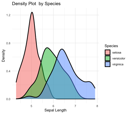
From Figure 1, it is clear that different species have different distributions of Sepal Length, suggesting that there might be dependence of sepal length on species. To confirm the same inference, we conduct the proposed hypothesis test on the data set. The calculated value of the JEL ratio $-2\log R(\Delta)=78.55$. The result suggests that we can reject the null hypothesis at 5% as well as 1% significance level. Thus, as per the test, we can conclude that Sepal length of the Iris flower is dependent on species.

5. Conclusion

The Test for independence between random variables is very useful in multiple applications. There are several tests for independence available if $X$ and $Y$ are continuous. In view of the recently introduced measure ’categorical Gini correlation’, we develop a U-statistics based test for testing the independence between a categorical variable and a continuous variable. We employed the JEL ratio test for testing the same as the usual normality-based test was difficult. The simulation study revealed that the proposed JEL ratio test has a well-controlled type I error and has good power for various choices of alternatives. We illustrated the test procedure using the famous Iris data set.

References

  • [1] Beknazaryan, A., Dang, X. & Sang, H. (2019). On mutual information estimation for mixed-pair random variables. Statistics & Probability Letters, 148, 9–16.
  • [2] Dang, X., Sang, H. & Weatherall, L. (2019). Gini covariance matrix and its affine equivariant version. Statistical Papers, 60, 641–666.
  • [3] Dang, X., Nguyen, D. Chen, Y. & Zhang, J. (2021). A new Gini correlation between quantitative and qualitative variables. Scandinavian Journal of Statistics, 48, 1314–1343.
  • [4] Gibbons, J. D. (1993). Nonparametric Measures of Association, Sage.
  • [5] Hewage, S. & Sang, Y. (2024). Jackknife empirical likelihood confidence intervals for the categorical Gini correlation. Journal of Statistical Planning and Inference, 231, 106–123.
  • [6] Jing, B. Y., Yuan, J. & Zhou, W. (2009). Jackknife empirical likelihood. Journal of the American Statistical Association, 104, 1224–1232.
  • [7] Lee, A. J. (2019). U-statistics: Theory and Practice. Routledge, New York.
  • [8] Mari, D. D. & Kotz, S. (2001). Correlation and Dependence. World Scientific.
  • [9] Owen, A. B. (1988). Empirical likelihood ratio confidence intervals for a single functional. Biometrika, 75, 237–249.
  • [10] Owen, A. (1990). Empirical likelihood ratio confidence regions. The Annals of Statistics, 18, 90–120.
  • [11] Sang, Y., Dang, X. & Zhao, Y. (2021). A jackknife empirical likelihood approach for K‐sample tests.Canadian Journal of Statistics, 49, 1115–1135.
  • [12] Sen, P. K. (1960). On some convergence properties of U-statistics. Calcutta Statistical Association Bulletin, 10, 1–18.
  • [13] Shevlyakov, G. & Smirnov, P. (2011). Robust estimation of the correlation coefficient: An attempt of survey. Austrian Journal of Statistics, 40, 147–156.
  • [14] Thomas, D. R. & Grunkemeier, G. L. (1975). Confidence interval estimation of survival probabilities for censored data. Journal of the American Statistical Association, 70, 865–871.